

Urban Street Network Configuration and Property Crime: An Empirical Multivariate Case Study


Abstract
1. Introduction
2. Literature Review
2.1. Theoretical Framework
2.2. Empirical Studies on Street Network Configuration and Crime Analysis
3. Study Area, Data, and Methods
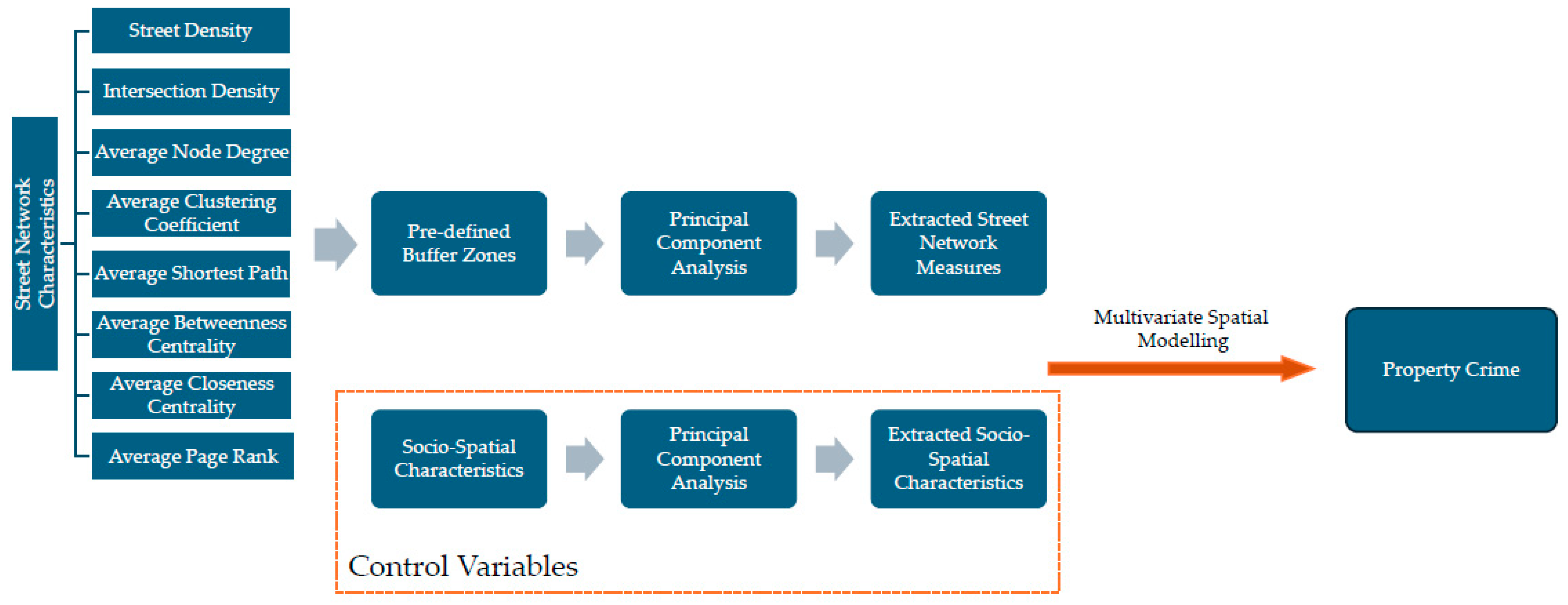
3.1. Overall Research Design
3.2. Case Study
3.3. Data
3.3.1. Overview
3.3.2. Property Crime Data
3.3.3. Street Network Configuration
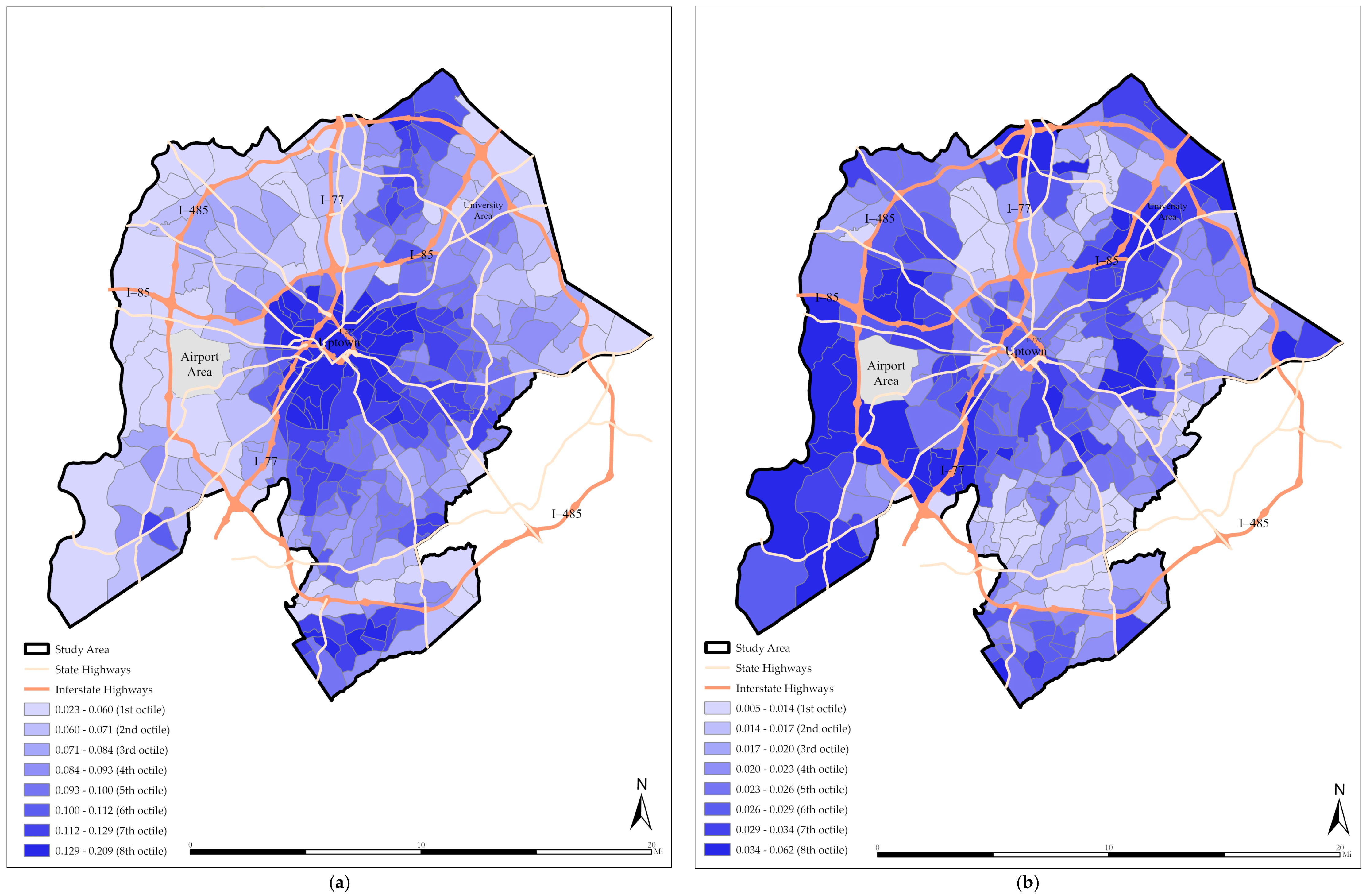
- Street Density (SD): This measures the total length of street segments within an NPA network divided by the areal size of the NPA. It captures the packing of the street infrastructure in the neighborhood. A higher density reflects a more accessible urban environment [69].
- Intersection Density (ID): As a second measure of network density, this represents the concentration of intersections in an NPA. It is calculated by dividing the number of nodes with a degree of three or more (indicating intersections) in the network by the NPA. Higher intersection density is associated with smaller block sizes, reflecting more interconnected streets [70].
- Average Node Degree (AND): This measure takes each street intersection (node) in each NPA and examines how strongly it is connected to other nodes. Specifically, it counts the number of street links (edges) incident at each node, defined as the node degree. The AND is the average of node degrees in each NPA. Higher AND values denote a more interconnected network, where nodes have more direct street connections [56].
- Average Clustering Coefficient (ACC): This reflects the indirect adjacent connectivity and the degree to which nodes in the network cluster together. Practically, the clustering coefficient of a node is defined as the ratio of the number of neighbor nodes connected to each other to the total number of possible connections between them [71]. The ACC averages these values over all nodes in an NPA. A higher ACC would describe a network with localized clusters, supporting short-range connectivity [72].
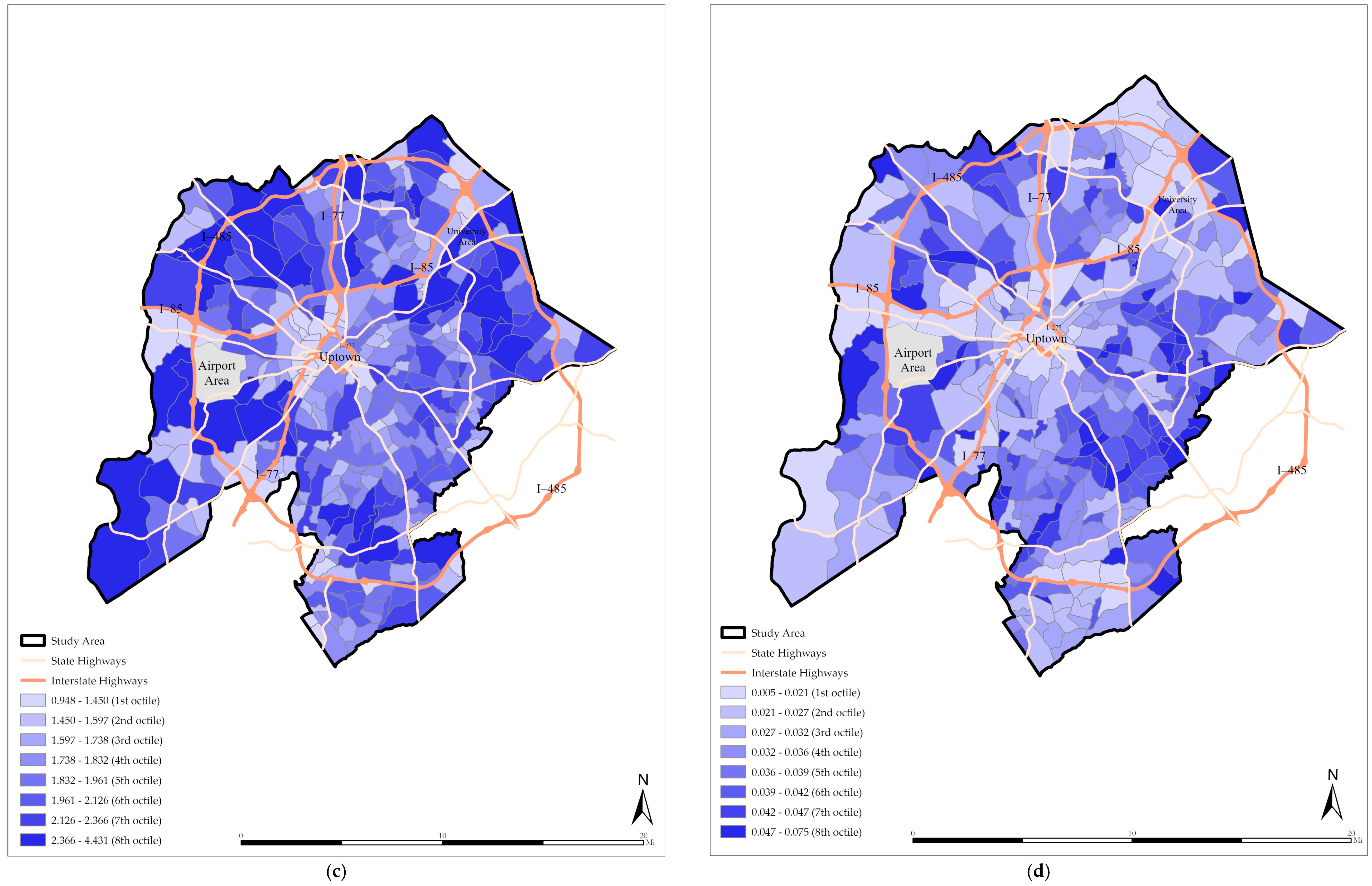
- Average Shortest Path (ASP): This is calculated by the average of paths with the shortest distance to travel between all pairs of nodes in the NPA network. A shorter ASP enhances local network accessibility [73].
- Average Betweenness Centrality (ABCe): The betweenness centrality quantifies how often a node acts as a bridge along the shortest path between any two other nodes [74]. Thus, a node with high betweenness value lies on many shortest paths between other nodes [75]. In this study, we measure the average betweenness value of nodes in an NPA network. Higher ABCe indicates a higher degree of interconnectedness of the local street network.
- Average Closeness Centrality (ACCe): This measure captures the extent to which nodes are close to all other nodes in a network, emphasizing the efficiency of interaction within the network [76]. Thus, a node with a high closeness value has a short path to all other nodes in the network, locating it at intersections that are central to the network’s structure [77]. The ACCe is the average of all nodes in the NPA network.
- Average Page Rank (APR): Page rank centrality focuses on the quantity, i.e., the degree of a node, and quality, i.e., the degree of nodes connected to that node of interest [78]. It concentrates on the direct and indirect role of a node in the network to determine its overall influence on its neighbors. Therefore, a node with a high page rank value has a high direct and indirect connectivity impact on the network. The APR averages the page rank centrality values of nodes in an NPA. A higher APR suggests more nodes play a central role in directly and indirectly connecting parts of the network.
3.3.4. Controlling for Socio-Spatial Characteristics
3.4. Multivariate Methods
4. Results
5. Discussion
6. Conclusions
Author Contributions
Funding
Data Availability Statement
Conflicts of Interest
Appendix A
Appendix A.1

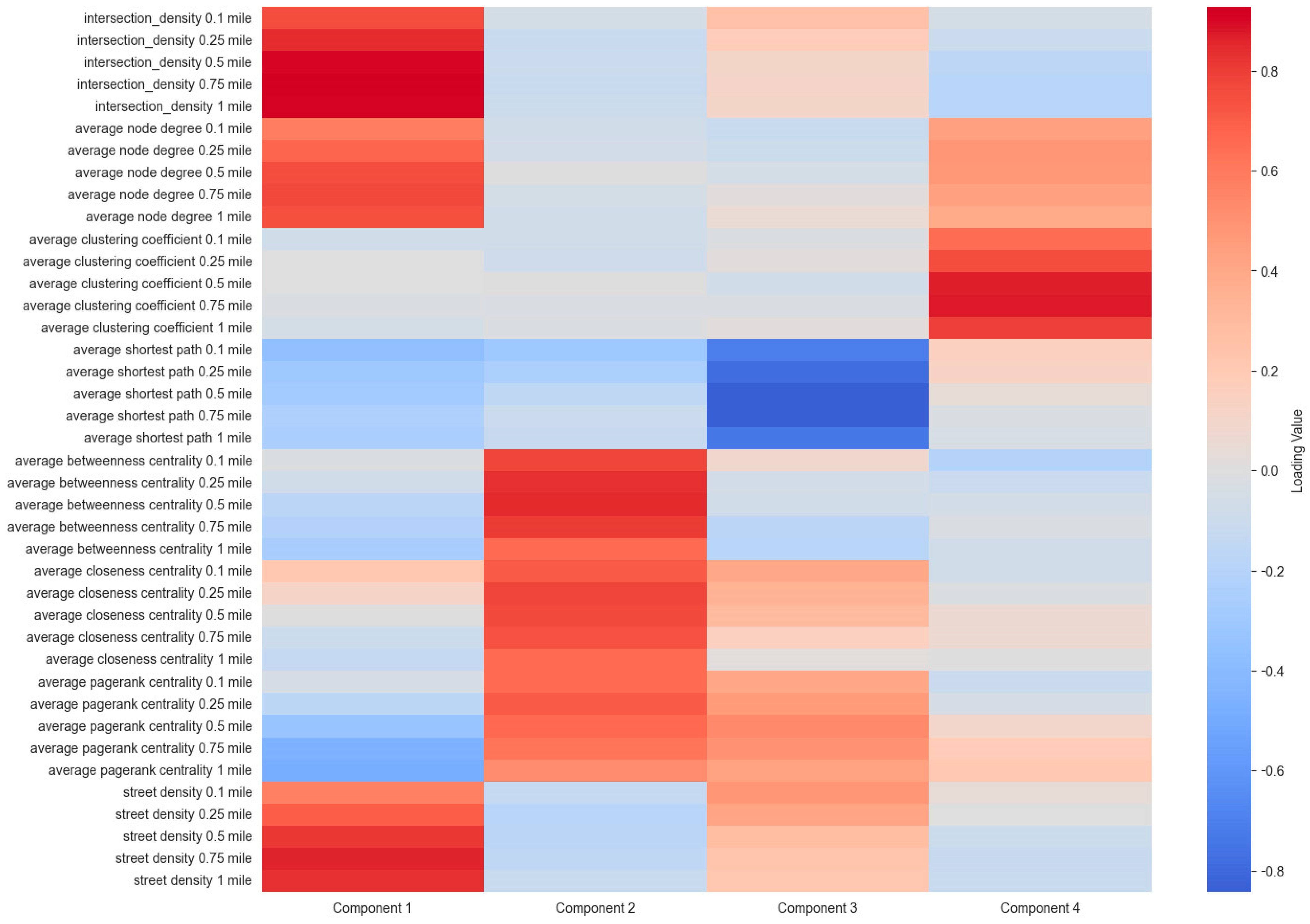
| Variable | Communality |
|---|---|
| Intersection Density 0.1 Mile | 0.635 |
| Intersection Density 0.25 Mile | 0.762 |
| Intersection Density 0.5 Mile | 0.861 |
| Intersection Density 0.75 Mile | 0.92 |
| Intersection Density 1 Mile | 0.88 |
| Average Node Degree 0.1 Mile | 0.542 |
| Average Node Degree 0.25 Mile | 0.695 |
| Average Node Degree 0.5 Mile | 0.788 |
| Average Node Degree 0.75 Mile | 0.788 |
| Average Node Degree 1 Mile | 0.717 |
| Average Clustering Coefficient 0.1 Mile | 0.428 |
| Average Clustering Coefficient 0.25 Mile | 0.585 |
| Average Clustering Coefficient 0.5 Mile | 0.754 |
| Average Clustering Coefficient 0.75 Mile | 0.762 |
| Average Clustering Coefficient 1 Mile | 0.627 |
| Average Shortest Path 0.1 Mile | 0.743 |
| Average Shortest Path 0.25 Mile | 0.779 |
| Average Shortest Path 0.5 Mile | 0.816 |
| Average Shortest Path 0.75 Mile | 0.776 |
| Average Shortest Path 1 Mile | 0.625 |
| Average Betweenness Centrality 0.1 Mile | 0.659 |
| Average Betweenness Centrality 0.25 Mile | 0.716 |
| Average Betweenness Centrality 0.5 Mile | 0.766 |
| Average Betweenness Centrality 0.75 Mile | 0.729 |
| Average Betweenness Centrality 1 Mile | 0.541 |
| Average Closeness Centrality 0.1 Mile | 0.715 |
| Average Closeness Centrality 0.25 Mile | 0.741 |
| Average Closeness Centrality 0.5 Mile | 0.683 |
| Average Closeness Centrality 0.75 Mile | 0.576 |
| Average Closeness Centrality 1 Mile | 0.447 |
| Average PageRank Centrality 0.1 Mile | 0.607 |
| Average PageRank Centrality 0.25 Mile | 0.744 |
| Average PageRank Centrality 0.5 Mile | 0.845 |
| Average PageRank Centrality 0.75 Mile | 0.871 |
| Average PageRank Centrality 1 Mile | 0.738 |
| Street Density 0.1 Mile | 0.57 |
| Street Density 0.25 Mile | 0.693 |
| Street Density 0.5 Mile | 0.782 |
| Street Density 0.75 Mile | 0.829 |
| Street Density 1 Mile | 0.769 |
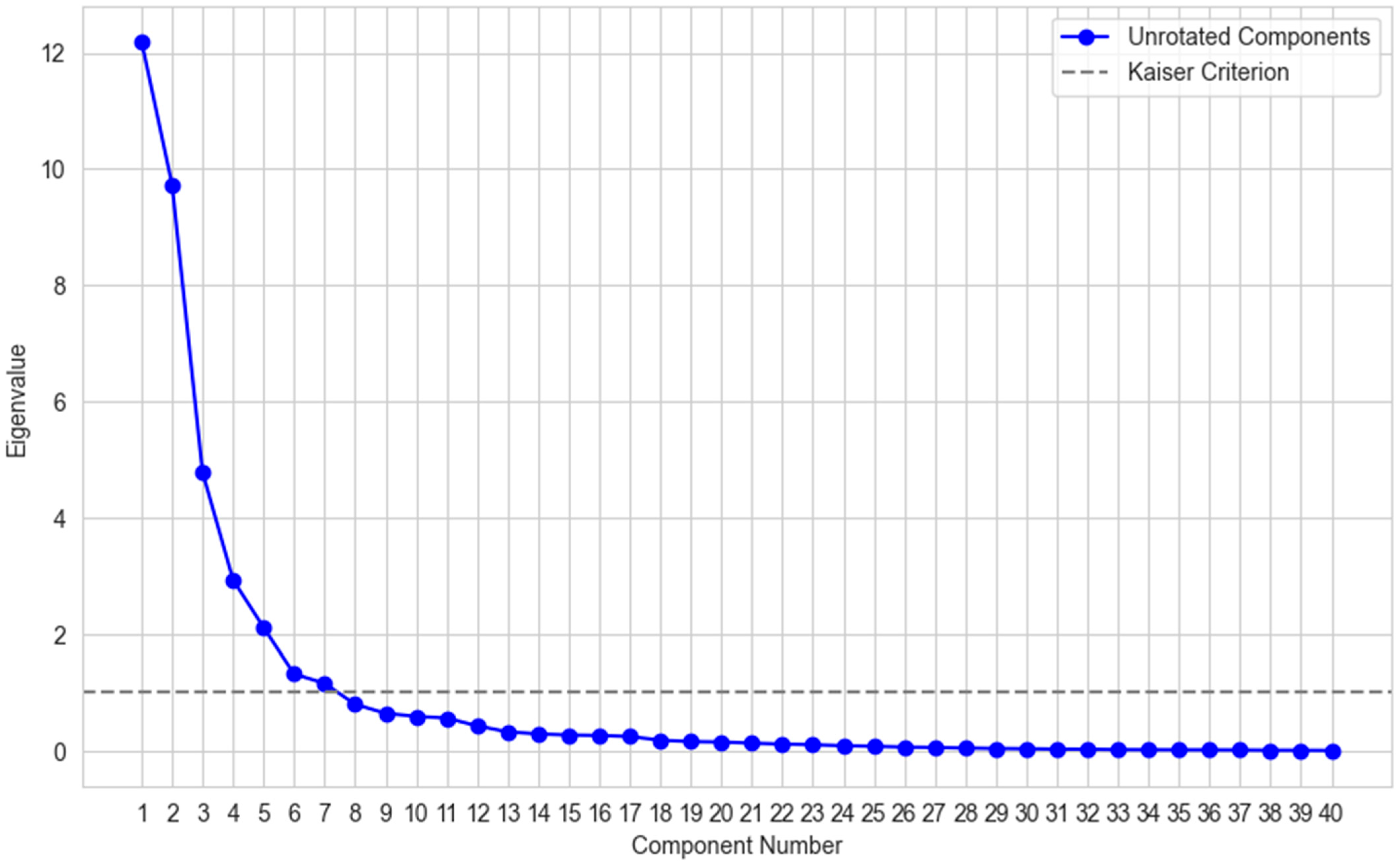
| Component | Share of Variance |
|---|---|
| Component 1 | 0.26 |
| Component 2 | 0.20 |
| Component 3 | 0.13 |
| Component 4 | 0.11 |
| Total | 0.70 |
Appendix A.2

| Variable | Communality |
|---|---|
| Percentage of Over 25-Year-Olds With a Bachelor’s Degree | 0.869 |
| Employment Rate | 0.995 |
| Home Ownership Rate | 0.883 |
| Residential Occupancy | 0.995 |
| Percentage of Single-Family House Among All Housing | 0.804 |
| Average Age of Single-Family Housing | 0.406 |
| Housing Density | 0.523 |
| Average Size of Single-Family Housing | 0.730 |
| Average Sales Price of Homes | 0.593 |
| Median Age of Residents | 0.536 |
| Median Household Income | 0.808 |
| Percentage of Population That Identify as Hispanic | 0.995 |
| Percentage of Population That Identify as Asian | 0.625 |
| Percentage of Population That Identify as Black | 1.003 |
| Percentage of Population That Identify as White | 0.996 |
| Total Heated Square Footage | 0.238 |
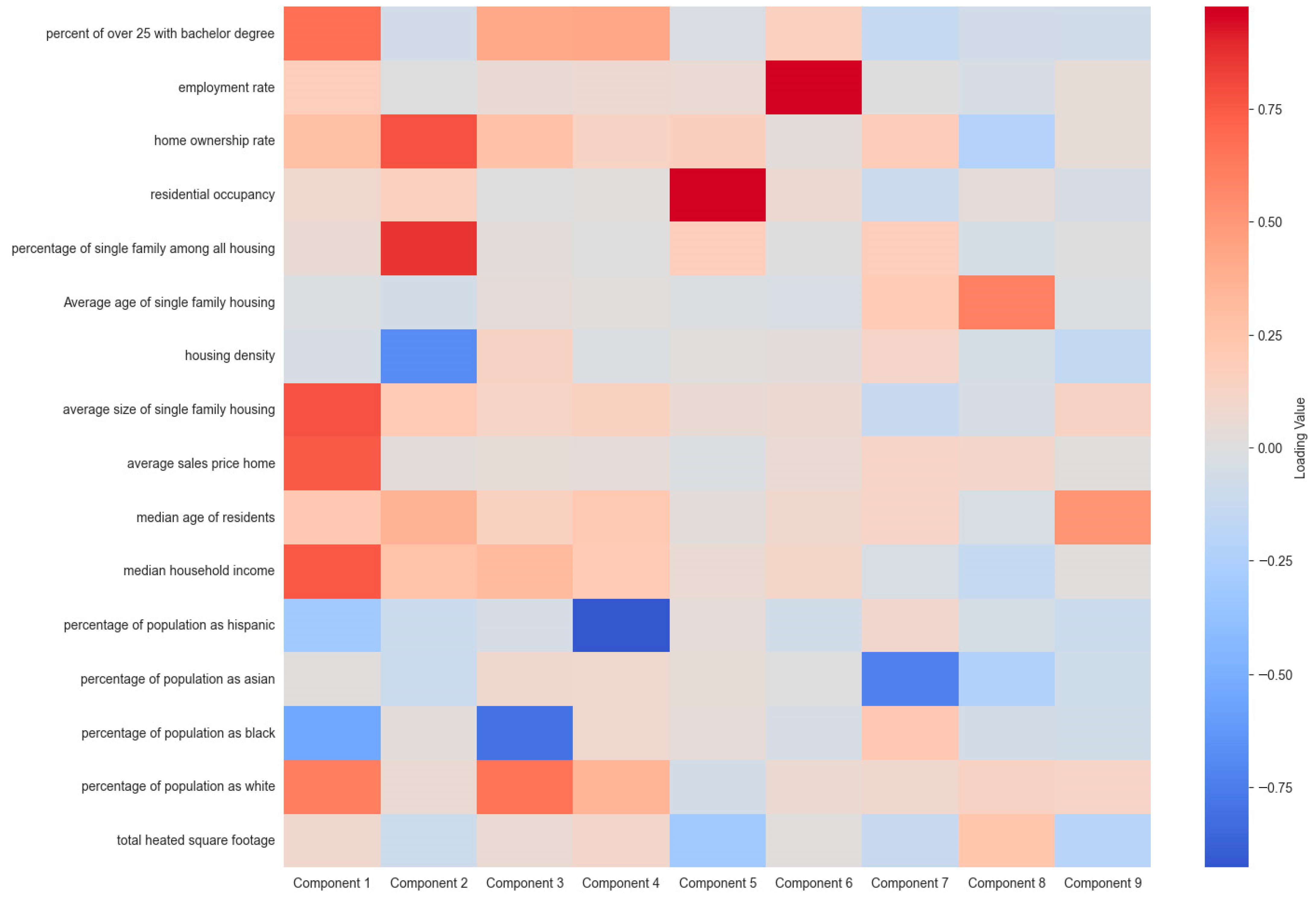
| Component | Share of Variance |
|---|---|
| Component 1 | 0.19 |
| Component 2 | 0.13 |
| Component 3 | 0.09 |
| Component 4 | 0.08 |
| Component 5 | 0.06 |
| Component 6 | 0.06 |
| Component 7 | 0.05 |
| Component 8 | 0.03 |
| Component 9 | 0.02 |
| Total | 0.71 |
References
- Mara, F.; Cutini, V. The Environmental Approach to Security: A Historical-Theoretical Literature Review on Space and Crime. Plan. Theory Pract. 2024, 25, 525–547. [Google Scholar] [CrossRef]
- van Soomeren, P. Tackling crime and fear of crime through urban planning and Architectural Design. Crime Prev. Environ. Des. 2013, 3, 219–272. [Google Scholar]
- Ceccato, V. The Urban Fabric of Crime and Fear. In The Urban Fabric of Crime and Fear; Ceccato, V., Ed.; Springer: Dordrecht, The Netherlands, 2012; pp. 1–33. ISBN 978-94-007-4210-9. [Google Scholar]
- Bernasco, W.; Block, R. Robberies in Chicago: A Block-Level Analysis of the Influence of Crime Generators, Crime Attractors, and Offender Anchor Points. J. Res. Crime Delinq. 2011, 48, 33–57. [Google Scholar] [CrossRef]
- Brantingham, P.; Brantingham, P. Criminality of Place: Crime Generators and Crime Attractors. Eur. J. Crim. Policy Res. 1995, 3, 5–26. [Google Scholar] [CrossRef]
- Shalev, K. Strategies Property Offenders Use in Spatial Decision Making. Ph.D. Thesis, University of Liverpool, Liverpool, UK, 2004. Available online: https://livrepository.liverpool.ac.uk/3174839/1/408559.pdf (accessed on 25 November 2024).
- Van Daele, S.; Beken, T.V. Outbound offending: The journey to crime and crime sprees. J. Environ. Psychol. 2011, 31, 70–78. [Google Scholar] [CrossRef]
- Kim, Y.-A.; Hipp, J.R. Pathways: Examining Street Network Configurations, Structural Characteristics and Spatial Crime Patterns in Street Segments. J. Quant. Criminol. 2020, 36, 725–752. [Google Scholar] [CrossRef]
- Haider, M.; Iamtrakul, P. Theoretical Concepts of Crime and Practices in Urban Planning and Design Process for Safe Urban Life. Int. J. Build. Urban Inter. Landsc. Technol. 2018, 12, 7–24. [Google Scholar]
- Mao, Y.; Yin, L.; Zeng, M.; Ding, J.; Song, Y. Review of Empirical Studies on Relationship between Street Environment and Crime. J. Plan. Lit. 2021, 36, 187–202. [Google Scholar] [CrossRef]
- Summers, L.; Johnson, S.D. Does the Configuration of the Street Network Influence Where Outdoor Serious Violence Takes Place? Using Space Syntax to Test Crime Pattern Theory. J. Quant. Criminol. 2017, 33, 397–420. [Google Scholar] [CrossRef]
- Duffee, D.; McDowall, D.; Mazerolle, L.G.; Mastrofski, S.D. Measurement and Analysis of Crime and Justice: An Introductory Essay. Crim. JUSTICE 2000, 4, 1–31. Available online: https://nij.ojp.gov/library/publications/measurement-and-analysis-crime-and-justice-introductory-essay (accessed on 12 December 2024).
- Astengo, G. Urbanistica; Istituto Perla Collaborazione Culturale: Rome, Italy, 1971; Available online: https://webapps.unitn.it/Biblioteca/it/Web/EngibankFile/1953indice%2013.pdf (accessed on 18 October 2024).
- Cozens, P.; Love, T. A Review and Current Status of Crime Prevention through Environmental Design (CPTED). J. Plan. Lit. 2015, 30, 393–412. [Google Scholar] [CrossRef]
- Plucknett, T. Edward I and Criminal Law/by TFT Plucknett; Cambridge [Cambridgeshire] University Press: Cambridge, UK, 1960. [Google Scholar]
- Dyos, H.J. Urban Transformation: A Note on the Objects of Street Improvement in Regency and Early Victorian London. Int. Rev. Soc. Hist. 1957, 2, 259–265. [Google Scholar] [CrossRef]
- Tobias, J.J. Urban Crime in Victorian England; Schocken Books: New York, NY, USA, 1967. [Google Scholar]
- Fortunati, V. Le Città Utopiche tra Immaginazione e Storia. 2003. Available online: http://hdl.handle.net/10077/7135 (accessed on 15 December 2024).
- Beirne, P. Adolphe Quetelet and the Origins of Positivist Criminology. Am. J. Sociol. 1987, 92, 1140–1169. [Google Scholar] [CrossRef]
- Bellair, P. Social Disorganization Theory. In Oxford Research Encyclopedia of Criminology; Oxford University Press: Oxford, UK, 2017; ISBN 978-0-19-026407-9. Available online: https://oxfordre.com/criminology/display/10.1093/acrefore/9780190264079.001.0001/acrefore-9780190264079-e-253 (accessed on 2 September 2024).
- Gibson, V.L. Third Generation CPTED? Rethinking the Basis for Crime Prevention Strategies. Ph.D. Thesis, University of Northumbria, Newcastle, UK, 2016. Available online: https://www.proquest.com/docview/1864778307/abstract/31B5E90485D44DA2PQ/1 (accessed on 4 December 2024).
- Kornhauser, R.R. Social Sources of Delinquency: An Appraisal of Analytic Models. Ph.D. Thesis, The University of Chicago, Chicago, IL, USA, 1975. Available online: https://www.proquest.com/docview/302825154/citation/FBCA4F89FF60436CPQ/1 (accessed on 25 November 2024).
- Kubrin, C.E.; Wo, J.C. Social Disorganization Theory’s Greatest Challenge. In The Handbook of Criminological Theory; John Wiley & Sons, Ltd.: Hoboken, NJ, USA, 2015; pp. 121–136. ISBN 978-1-118-51244-9. [Google Scholar]
- Peck, J.H.; Leiber, M.J.; Beaudry-Cyr, M.; Toman, E.L. The Conditioning Effects of Race and Gender on the Juvenile Court Outcomes of Delinquent and “Neglected” Types of Offenders. Justice Q. 2016, 33, 1210–1236. [Google Scholar] [CrossRef]
- Dao, T.H.D.; Thill, J.-C. CrimeScape: Analysis of socio-spatial associations of urban residential motor vehicle theft. Soc. Sci. Res. 2022, 101, 102618. [Google Scholar] [CrossRef] [PubMed]
- Cozens, P.M. Urban Planning and Environmental Criminology: Towards a New Perspective for Safer Cities. Plan. Pract. Res. 2011, 26, 481–508. [Google Scholar] [CrossRef]
- Newman, O. Creating Defensible Space; DIANE Publishing: Darby, PA, USA, 1997; ISBN 978-0-7881-4528-5. [Google Scholar]
- Mayhew, P.; Clarke, R.V.G.; Sturman, A.; Hough, J.M. Crime as Opportunity; HM Stationery Office: London, UK, 1976; Volume 34, Available online: https://popcenter.asu.edu/sites/default/files/124-mayhew_et_al-crime_as_opportunity.pdf (accessed on 12 January 2025).
- Cohen, L.E.; Felson, M. Social Change and Crime Rate Trends: A Routine Activity Approach. Am. Sociol. Rev. 1979, 44, 588–608. [Google Scholar] [CrossRef]
- Wilson, J.Q.; Kelling, G. “Broken Windows” Critical Issues in Policing: Contemporary Readings. 1982. Available online: https://www.crimeconomics.com/s/BrokenWindows-AtlantaicMonthly-March82-xr78.pdf (accessed on 2 October 2024).
- Birks, D.; Davies, T. Street Network Structure and Crime Risk: An Agent-Based Investigation of the Encounter and Enclosure Hypotheses. Criminology 2017, 55, 900–937. [Google Scholar] [CrossRef]
- Beavon, D.J.; Brantingham, P.L.; Brantingham, P.J. The influence of street networks on the patterning of property offenses. Crime Prev. Stud. 1994, 2, 115–148. [Google Scholar]
- Hollis-Peel, M.E.; Welsh, B.C. What makes a guardian capable? A test of guardianship in action. Secur. J. 2014, 27, 320–337. [Google Scholar] [CrossRef]
- Ackerman, J.M.; Rossmo, D.K. How Far to Travel? A Multilevel Analysis of the Residence-to-Crime Distance. J. Quant. Criminol. 2015, 31, 237–262. [Google Scholar] [CrossRef]
- Baran, P.K.; Smith, W.R.; Toker, U. The space syntax and crime. In Proceedings of the 6th International Space Syntax Symposium, Istanbul, Turkey, 21–15 June 2007; Available online: http://spacesyntaxistanbul.itu.edu.tr/papers/shortpapers/119%20-%20Baran%20Smith%20Toker.pdf (accessed on 5 September 2024).
- Davies, T.; Johnson, S.D. Examining the Relationship Between Road Structure and Burglary Risk Via Quantitative Network Analysis. J. Quant. Criminol. 2015, 31, 481–507. [Google Scholar] [CrossRef]
- Davison, E.; Smith, W. Exploring accessibility versus opportunity crime factors. Sociation Today J. N. C. Sociol. Assoc. 2003, 1, 1–9. Available online: https://libres.uncg.edu/ir/asu/f/Davison_Beth_2003_Exploring_Accessibility.pdf (accessed on 8 December 2024).
- Frith, M.J.; Johnson, S.D.; Fry, H.M. Role of the Street Network in Burglars’ Spatial Decision-Making. Criminology 2017, 55, 344–376. [Google Scholar] [CrossRef]
- Johnson, S.D.; Bowers, K.J. Permeability and Burglary Risk: Are Cul-de-Sacs Safer? J. Quant. Criminol. 2010, 26, 89–111. [Google Scholar] [CrossRef]
- Nutter, J.B.; Bevis, C. Changing Street Layouts to Reduce Residential Burglary; NCJ Number 51937; Minnesota Crime Prevention Center: Minneapolis, MN, USA, 1977. Available online: https://www.ojp.gov/pdffiles1/Digitization/51937NCJRS.pdf (accessed on 5 December 2024).
- White, G.F. Neighborhood permeability and burglary rates. Justice Q. 1990, 7, 57–67. [Google Scholar] [CrossRef]
- Eck, J.E.; Weisburd, D. Crime places in crime theory. Crime Place Crime Prev. Stud. 2015, 4, 1–33. Available online: https://papers.ssrn.com/sol3/Delivery.cfm/SSRN_ID2629856_code2377032.pdf?abstractid=2629856&mirid=1 (accessed on 5 February 2025).
- Rengert, G.F.; Wasilchick, J. Suburban Burglary: A Tale of Two Suburbs; Charles C. Thomas: Springfield, IL, USA, 2000. Available online: https://www.ojp.gov/ncjrs/virtual-library/abstracts/suburban-burglary-tale-two-suburbs-second-edition (accessed on 12 July 2024).
- Taylor, R.B.; Harrell, A. Physical Environment and Crime; US Department of Justice: Washington, DC, USA, 1996. [Google Scholar]
- Groff, E.R.; Taylor, R.B.; Elesh, D.B.; McGovern, J.; Johnson, L. Permeability across a Metropolitan Area: Conceptualizing and Operationalizing a Macrolevel Crime Pattern Theory. Environ. Plan. A 2014, 46, 129–152. [Google Scholar] [CrossRef]
- Weisburd, D.; Zastrow, T.; Kuen, K.; Andresen, M.A. Crime concentrations at micro places: A review of the evidence. Aggress. Violent Behav. 2024, 78, 101979. [Google Scholar] [CrossRef]
- Kronkvist, K. Placing Perceptions of Unsafety: Examining Spatial Concentrations and Temporal Patterns of Unsafe Locations at Micro-Places. J. Quant. Criminol. 2024, 40, 191–213. [Google Scholar] [CrossRef]
- Nepomuceno, T.C.C.; Costa, A.P.C.S. Spatial visualization on patterns of disaggregate robberies. Oper. Res. 2019, 19, 857–886. [Google Scholar] [CrossRef]
- Weisburd, D.; Groff, E.R.; Yang, S.-M. The Criminology of Place: Street Segments and Our Understanding of the Crime Problem, 1st ed.; Oxford University Press: Oxford, UK, 2012; ISBN 978-0-19-992863-7. [Google Scholar]
- Pratt, T.C.; Cullen, F.T. Assessing Macro-Level Predictors and Theories of Crime: A Meta-Analysis. Crime Justice 2005, 32, 373–450. [Google Scholar] [CrossRef]
- Rosa, A.G.F.; de Miranda Mota, C.M.; de Figueiredo, C.J.J. A spatial multi-criteria decision analysis framework to reveal vulnerabilities of areas to incidences of street robberies. Appl. Geogr. 2023, 151, 102840. [Google Scholar] [CrossRef]
- Stucky, T.D.; Ottensmann, J.R. Land Use and Violent Crime. Criminology 2009, 47, 1223–1264. [Google Scholar] [CrossRef]
- Browning, C.R.; Byron, R.A.; Calder, C.A.; Krivo, L.J.; Kwan, M.-P.; Lee, J.-Y.; Peterson, R.D. Commercial Density, Residential Concentration, and Crime: Land Use Patterns and Violence in Neighborhood Context. J. Res. Crime Delinq. 2010, 47, 329–357. [Google Scholar] [CrossRef]
- Lima, R.A.; Taques, F.H.; Nepomuceno, T.C.C.; de Figueiredo, C.J.J.; Poleto, T.; de Carvalho, V.D.H. Simultaneous Causality and the Spatial Dynamics of Violent Crimes as a Factor in and Response to Police Patrolling. Urban Sci. 2024, 8, 132. [Google Scholar] [CrossRef]
- U.S. Census Bureau. Population Estimates, Demographic Characteristics, and Economic Data for Charlotte, North Carolina. 2023. Available online: https://www.census.gov/quickfacts/fact/table/charlottecitynorthcarolina/PST045223 (accessed on 10 July 2024).
- Boeing, G. Urban spatial order: Street network orientation, configuration, and entropy. Appl. Netw. Sci. 2019, 4, 67. [Google Scholar] [CrossRef]
- CMPD. 2023 Annual Report; Charlotte-Mecklenburg Police Department: Charlotte, NC, USA, 2023. Available online: https://www.charlottenc.gov/files/sharedassets/police/v/1/newsroom/article_documents/cmpd-eoy-website-reduced.pdf (accessed on 10 September 2024).
- Federal Bureau of Investigation. Offense Definitions; Federal Bureau of Investigation: Washington, DC, USA, 2019. Available online: https://ucr.fbi.gov/crime-in-the-u.s/2019/crime-in-the-u.s.-2019/topic-pages/offense-definitions (accessed on 24 September 2024).
- Mecklenburg County Quality of Life Explorer 2022. Available online: https://mcmap.org/qol/#58/ (accessed on 1 March 2024).
- Mecklenburg County Mecklenburg County Tax Parcels with CAMA Data. 2024. Available online: https://maps.mecknc.gov/opendata/metadata/Tax_Parcels_with_CAMA_Data.html (accessed on 26 March 2024).
- Barthélemy, M. Spatial networks. Phys. Rep. 2011, 499, 1–101. [Google Scholar] [CrossRef]
- Boeing, G. OSMnx: New methods for acquiring, constructing, analyzing, and visualizing complex street networks. Comput. Environ. Urban Syst. 2017, 65, 126–139. [Google Scholar] [CrossRef]
- Boeing, G.D. Methods and Measures for Analyzing Complex Street Networks and Urban Form. Ph.D. Thesis, University of California, Berkeley, CA, USA, 2017. Available online: https://www.proquest.com/docview/1924684815/abstract/4EE07EF9CC55445BPQ/1 (accessed on 22 December 2024).
- Borgatti, S.P. Centrality and network flow. Soc. Netw. 2005, 27, 55–71. [Google Scholar] [CrossRef]
- Newman, M.E.J. A measure of betweenness centrality based on random walks. Soc. Netw. 2005, 27, 39–54. [Google Scholar] [CrossRef]
- Parthasarathi, P.; Levinson, D.; Hochmair, H. Network Structure and Travel Time Perception. PLoS ONE 2013, 8, e77718. [Google Scholar] [CrossRef] [PubMed]
- Parthasarathi, P.; Levinson, D. Network structure and the journey to work: An intra-metropolitan analysis. Transp. Res. Part Policy Pract. 2018, 118, 292–304. [Google Scholar] [CrossRef]
- Wang, F.; Antipova, A.; Porta, S. Street centrality and land use intensity in Baton Rouge, Louisiana. J. Transp. Geogr. 2011, 19, 285–293. [Google Scholar] [CrossRef]
- Boeing, G. A multi-scale analysis of 27,000 urban street networks: Every US city, town, urbanized area, and Zillow neighborhood. Environ. Plan. B Urban Anal. City Sci. 2020, 47, 590–608. [Google Scholar] [CrossRef]
- Bielik, M.; König, R.; Schneider, S.; Varoudis, T. Measuring the Impact of Street Network Configuration on the Accessibility to People and Walking Attractors. Netw. Spat. Econ. 2018, 18, 1–20. [Google Scholar] [CrossRef]
- Li, Y.; Shang, Y.; Yang, Y. Clustering coefficients of large networks. Inf. Sci. 2017, 382–383, 350–358. [Google Scholar] [CrossRef]
- Wang, Y.; Ghumare, E.; Vandenberghe, R.; Dupont, P. Comparison of Different Generalizations of Clustering Coefficient and Local Efficiency for Weighted Undirected Graphs. Neural Comput. 2017, 29, 313–331. [Google Scholar] [CrossRef]
- Labi, S.; Faiz, A.; Saeed, T.U.; Alabi, B.N.T.; Woldemariam, W. Connectivity, Accessibility, and Mobility Relationships in the Context of Low-Volume Road Networks. Transp. Res. Rec. 2019, 2673, 717–727. [Google Scholar] [CrossRef]
- Brandes, U. A faster algorithm for betweenness centrality. J. Math. Sociol. 2001, 25, 163–177. [Google Scholar] [CrossRef]
- Bergamini, E.; Crescenzi, P.; D’angelo, G.; Meyerhenke, H.; Severini, L.; Velaj, Y. Improving the Betweenness Centrality of a Node by Adding Links. ACM J. Exp. Algorithmics 2018, 23, 1–32. [Google Scholar] [CrossRef]
- Crucitti, P.; Latora, V.; Porta, S. Centrality in networks of urban streets. Chaos Interdiscip. J. Nonlinear Sci. 2006, 16, 015113. [Google Scholar] [CrossRef]
- Chen, H.-H.; Dietrich, U. Normalized closeness centrality of urban networks: Impact of the location of the catchment area and evaluation based on an idealized network. Appl. Netw. Sci. 2023, 8, 60. [Google Scholar] [CrossRef]
- Bowater, D.; Stefanakis, E. Extending the Adapted PageRank Algorithm centrality model for urban street networks using non-local random walks. Appl. Math. Comput. 2023, 446, 127888. [Google Scholar] [CrossRef]
- Batty, M.; Longley, P. Fractal Cities: A Geometry of Form and Function, 1st ed.; Academic Press: London, UK, 1994; ISBN 978-0-12-455570-9. [Google Scholar]
- Kansky, K.J. Structure of Transportation Networks: Relationships Between Network Geometry and Regional Characteristics; University of Chicago: Chicago, IL, USA, 1963. [Google Scholar]
- Watts, D.J.; Strogatz, S.H. Collective dynamics of ‘small-world’ networks. Nature 1998, 393, 440–442. [Google Scholar] [CrossRef] [PubMed]
- Granovetter, M.S. The Strength of Weak Ties. Am. J. Sociol. 1973, 78, 1360–1380. [Google Scholar] [CrossRef]
- Freeman, L.C. A Set of Measures of Centrality Based on Betweenness. Sociometry 1977, 40, 35–41. [Google Scholar] [CrossRef]
- Bavelas, A. Communication Patterns in Task-Oriented Groups. J. Acoust. Soc. Am. 1950, 22, 725–730. [Google Scholar] [CrossRef]
- Page, L. The PageRank Citation Ranking: Bringing Order to the Web; Technical Report; Stanford infolab: Stanford, CA, USA, 1998. [Google Scholar]
- Mecklenburg County Street Centerline in Mecklenburg County 2023. Available online: https://maps.mecknc.gov/opendata/metadata/Street_Centerline.html (accessed on 8 May 2025).
- Kadar, C.; Feuerriegel, S.; Noulas, A.; Mascolo, C. Leveraging Mobility Flows from Location Technology Platforms to Test Crime Pattern Theory in Large Cities. arXiv 2020, arXiv:2004.08263. [Google Scholar] [CrossRef]
- O’Leary, M. Modeling Criminal Distance Decay. Cityscape 2011, 13, 161–198. [Google Scholar]
- Rossmo, D.K.; Wheeler, A. The Journey-to-Crime Buffer Zone: Measurement Issues and Methodological Challenges. CrimRxiv 2024, 95, 102272. [Google Scholar] [CrossRef]
- Babaey, V.; Ravindran, A. GenSQLi: A Generative Artificial Intelligence Framework for Automatically Securing Web Application Firewalls Against Structured Query Language Injection Attacks. Future Internet 2025, 17, 8. [Google Scholar] [CrossRef]
- Fan, J.; Sun, Q.; Zhou, W.-X.; Zhu, Z. Principal component analysis for big data. arXiv 2018, arXiv:1801.01602. [Google Scholar] [CrossRef]
- Janicijevic, S.; Mizdrakovic, V.; Kljajić, M. Principal Component Analysis in Financial Data Science. In Advances in Principal Component Analysis; IntechOpen: London, UK, 2022; ISBN 978-1-80355-765-6. [Google Scholar] [CrossRef]
- Mavungu, M. Computation of financial risk using principal component analysis. Algorithmic Financ. 2023, 10, 1–20. [Google Scholar] [CrossRef]
- Cossu, G.; Agus, M.; Atzori, L.; Aviles Gonzales, C.I.; Minerba, L.; Ferreli, C.; Puxeddu, R.; Orrù, G.; Scano, A.; Romano, F.; et al. Principal Component Analysis of the Social and Behavioral Rhythms Scale in elderly. J. Public Health Res. 2022, 11, jphr-2021. [Google Scholar] [CrossRef] [PubMed]
- Magyar, Z.B. What Makes Party Systems Different? A Principal Component Analysis of 17 Advanced Democracies 1970–2013. Polit. Anal. 2022, 30, 250–268. [Google Scholar] [CrossRef]
- U.S. Census Bureau. American Community Survey 2015–2019, 5-Year Estimates; U.S Census Bureau: Washington, DC, USA, 2019.
- Minnesota Population Center. National Historical Geographic Information System. Available online: https://www.nhgis.org (accessed on 26 June 2024).
- U.S. Census Bureau. Decennial Census: Summary File 1, QT-P3. Available online: https://www.census.gov/programs-surveys/decennial-census/about/rdo/summary-files.2010.html (accessed on 20 June 2024).
- Gelman, A. Data Analysis Using Regression and Multilevel/Hierarchical Models; Cambridge University Press: Cambridge, UK, 2007; Available online: https://www.cambridge.org/highereducation/books/data-analysis-using-regression-and-multilevel-hierarchical-models/32A29531C7FD730C3A68951A17C9D983#overview (accessed on 10 November 2024).
- Venables, W.N.; Ripley, B.D. Modern Applied Statistics with S; Springer Science & Business Media: Berlin/Heidelberg, Germany, 2003; ISBN 978-0-387-95457-8. [Google Scholar]
- Lindgren, F.; Rue, H. Bayesian Spatial Modelling with R-INLA. J. Stat. Softw. 2015, 63, 1–25. Available online: http://www.jstatsoft.org/v63/i19 (accessed on 20 May 2024). [CrossRef]
- Fotheringham, A.S.; Brunsdon, C.; Charlton, M.E. Geographically Weighted Regression: The Analysis of Spatially Varying Relationships; Wiley: Hoboken, NJ, USA, 2002; Available online: https://www.wiley.com/en-us/Geographically+Weighted+Regression%3A+The+Analysis+of+Spatially+Varying+Relationships+-p-9780471496168 (accessed on 1 June 2024).
- de Vries, I.; Davies, T. Understanding the role of street network configurations in the placement of illegitimately operating facilities. Criminology 2024, 62, 412–453. [Google Scholar] [CrossRef]
- Hatten, D.; Piza, E.L. When Crime Moves Where Does It Go? Analyzing the Spatial Correlates of Robbery Incidents Displaced by a Place-based Policing Intervention. J. Res. Crime Delinq. 2022, 59, 128–162. [Google Scholar] [CrossRef]
- Cozens, P.; Love, T. Manipulating Permeability as a Process for Controlling Crime: Balancing Security and Sustainability in Local Contexts. Built Environ. 2009, 35, 346–365. [Google Scholar] [CrossRef]
- Jamalishahni, T.; Davern, M.; Villanueva, K.; Turrell, G.; Foster, S. The contribution of objective and perceived crime to neighbourhood socio-economic inequity in loneliness. Health Place 2024, 85, 103165. [Google Scholar] [CrossRef]
- O’Sullivan, D. Too much of the wrong kind of data. Implications for the practice of micro-scale spatial modeling. In Spatially Integrated Social Science; Oxford University Press: Oxford, UK, 2004; pp. 95–108. [Google Scholar]
- Hipp, J.R. Block, Tract, and Levels of Aggregation: Neighborhood Structure and Crime and Disorder as a Case in Point. Am. Sociol. Rev. 2007, 72, 659–680. [Google Scholar] [CrossRef]
- Taylor, R.B. Community Criminology: Fundamentals of Spatial and Temporal Scaling, Ecological Indicators, and Selectivity Bias; New York University Press: New York, NY, USA, 2015; ISBN 978-0-8147-2549-8. [Google Scholar]
- Dao, T.H.D.; Thill, J.-C. The SpatialARMED Framework: Handling Complex Spatial Components in Spatial Association Rule Mining. Geogr. Anal. 2016, 48, 248–274. [Google Scholar] [CrossRef]
- Dong, Z.; Mateu, J.; Xie, Y. Spatio-Temporal-Network Point Processes for Modeling Crime Events with Landmarks. arXiv 2024, arXiv:2409.10882. [Google Scholar] [CrossRef]
- Shiode, S.; Shiode, N. Network-based space-time search-window technique for hotspot detection of street-level crime incidents. Int. J. Geogr. Inf. Sci. 2013, 27, 866–882. [Google Scholar] [CrossRef]
- Lee, S.; Chang, W.; Mateu, J.; Lee, H.; Park, J. A Spatio-Temporal Dirichlet Process Mixture Model on Linear Networks for Crime Data. arXiv 2025, arXiv:2501.08673. [Google Scholar] [CrossRef]


| Metric Name | Description | Equation | Reference |
|---|---|---|---|
| Street Density (SD) | = Total length of streets = Area | [69] | |
| Intersection Density (ID) | = Count of intersections = Area | [79] | |
| Average Node Degree (AND) | = Degree of node = Count of nodes | [80] | |
| Average Clustering Coefficient (ACC) | = Number of edges between the neighbors of node = Degree of node = Count of nodes | [81] | |
| Average Shortest Path (ASP) | d(i,j) = Shortest path distance between node i and node j = Count of nodes | [82] | |
| Average Betweenness Centrality (ABCe) | = Number of shortest paths between to Number of shortest paths between to that pass through node . = Count of nodes | [83] | |
| Average Closeness Centrality (ACCe) | d(i,j) = Shortest path distance between node i and node j = Count of nodes | [84] | |
| Average Page Rank (APR) | d = Damping factor N = Total number of nodes in the network M(i) = Set of nodes that link to node i PR(j) = PageRank of node j, which links to node i L(j) = Number of outbound links from node j | [85] |
| No. | Street Network Variable |
|---|---|
| 1 | Intersection density with 0.75-mile buffer zone |
| 2 | Average clustering coefficient with 0.75-mile buffer zone |
| 3 | Average shortest path with 0.75-mile buffer zone |
| 4 | Average betweenness centrality with 0.5-mile buffer zone |
| Street Network Variable | Mean | Std. Deviation | Median | Min. | Max. | Std. Error |
|---|---|---|---|---|---|---|
| Intersection density with 0.75-mile buffer zone | 0.034 | 0.011 | 0.0355 | 0.005 | 0.072 | 0.000 |
| Average clustering coefficient with 0.75-mile buffer zone | 0.089 | 0.029 | 0.088 | 0.023 | 0.190 | 0.001 |
| Average shortest path with 0.75-mile buffer zone | 0.023 | 0.009 | 0.023 | 0.005 | 0.060 | 0.000 |
| Average betweenness centrality with 0.5-mile buffer zone | 1.050 | 0.151 | 1.040 | 0.666 | 1.692 | 0.007 |
| Name | Definition | Source |
|---|---|---|
| Education Level | Population age 25 or older with a bachelor’s degree or higher divided by total population age 25 or older | [96] |
| Age of Residents | Median age of residents | [96] |
| Employment Rate | Number of individuals aged 16 to 64 in the civilian labor force and employed divided by the number of individuals ages 16 to 64 in the civilian labor force | [96] |
| Hispanic Population | Percentage of population self-identified as Hispanic or Latino | [97,98] |
| Asian Population | Percentage of population self-identified as Asian | [97,98] |
| Black Population | Percentage of population self-identified as Black | [97,98] |
| White Population | Percentage of population self-identified as White | [97,98] |
| Household Income | Inflation-adjusted median household income | [96] |
| Home Ownership | Number of owner-occupied housing units divided by the total number of occupied housing units | [96] |
| Residential Occupancy | Number of occupied housing units divided by the total number of housing units | [96] |
| Single-Family Housing Rate * | Number of single-family units divided by total housing units for the fiscal year | [60] |
| Average Age of Single-Family Housing * | Sum of each single-family housing structure age (year of data collection minus year structure built) divided by the total number of single-family housing structures | [60] |
| Housing Density | Number of housing units divided by total land area in acres | [60] |
| Average Size of Single-Family Housing * | Sum of heated square footage of all single-family housing units divided by the number of single-family housing units | [60] |
| Average Home Sales Price | Sum of sales values for single-family dwellings, condominiums, and townhomes divided by number of sales (data are cumulative for the previous two fiscal years) | [60] |
| Total Heated Square Footage | Sum of heated square footage of all building structures | [60] |
| No. | Socio-Spatial Components |
|---|---|
| 1 | Population affluence |
| 2 | Single-family housing |
| 3 | Caucasian and non-Black residents |
| 4 | Hispanic residents |
| 5 | Residential occupancy |
| 6 | Employment rate |
| 7 | Non-Asian residents |
| 8 | Age of single-family housing |
| 9 | Median age of residents |
| Variable | VIF Value |
|---|---|
| Average betweenness centrality | 1.24 |
| Intersection density | 1.42 |
| Average clustering coefficient | 1.15 |
| Average shortest path | 1.19 |
| Component 1 | 1.07 |
| Component 2 | 1.31 |
| Component 3 | 1.08 |
| Component 4 | 1.17 |
| Component 5 | 1.05 |
| Component 6 | 1.02 |
| Component 7 | 1.17 |
| Component 8 | 1.16 |
| Component 9 | 1.18 |
| Variable | Estimate | SE | z-Value | p-Value |
|---|---|---|---|---|
| Intercept | −2.105 | 0.338 | −6.216 | 0.000 |
| Average betweenness centrality 1 | −1.862 | 3.172 | −0.587 | 0.557 |
| Intersection density | 8.660 | 1.303 | 6.643 | 0.000 |
| Average clustering coefficient | 10.073 | 3.781 | 2.664 | 0.007 |
| Average shortest path | −0.887 | 0.235 | −3.767 | 0.000 |
| Component 1 | −0.308 | 0.037 | −8.270 | 0.000 |
| Component 2 | −0.586 | 0.038 | −15.146 | 0.000 |
| Component 3 | −0.223 | 0.036 | −6.151 | 0.000 |
| Component 4 | −0.216 | 0.035 | −6.107 | 0.000 |
| Component 5 | −0.096 | 0.033 | −2.908 | 0.003 |
| Component 6 | 0.033 | 0.033 | 1.010 | 0.312 |
| Component 7 | −0.034 | 0.014 | −2.363 | 0.018 |
| Component 8 | 0.156 | 0.046 | 3.386 | 0.000 |
| Component 9 | −0.019 | 0.050 | −0.387 | 0.698 |
| Model Fit | ||||
| Log-likelihood | AIC | Adjusted pseudo-R-squared | ||
| −1805.567 | 3641.1 | 0.47 | ||
| Spatial Diagnostics | ||||
| Test | Value | Std. deviations | p-value | |
| Moran’s I on dependent variable | 0.179 | 6.759 | 0.000 | |
| Moran’s I on residuals | 0.103 | 3.547 | 0.000 | |
| Variable | Mean | SD | 0.025 Quantile | 0.5 Quantile | 0.975 Quantile |
|---|---|---|---|---|---|
| Intercept | −2.307 | 1.251 | −4.763 | −2.308 | 0.150 |
| Average betweenness centrality 1 | −3.134 | 3.526 | −10.067 | −3.129 | 3.768 |
| Intersection density | 8.487 | 1.888 | 4.773 | 8.490 | 12.183 |
| Average clustering coefficient | 2.156 | 4.411 | −6.532 | 2.168 | 10.780 |
| Average shortest path | −1.114 | 1.014 | −3.095 | −1.116 | 0.880 |
| Component 1 | −0.006 | 0.558 | −1.093 | −0.017 | 1.141 |
| Component 2 | 0.168 | 0.530 | −0.801 | 0.136 | 1.307 |
| Component 3 | −0.024 | 0.521 | −1.065 | −0.026 | 1.024 |
| Component 4 | 0.953 | 0.522 | 0.025 | 0.913 | 2.080 |
| Component 5 | 0.770 | 0.562 | −0.283 | 0.746 | 1.950 |
| Component 6 | 0.047 | 0.489 | −0.933 | 0.047 | 1.031 |
| Component 7 | −0.059 | 0.232 | −0.559 | −0.050 | 0.383 |
| Component 8 | −1.154 | 0.571 | −2.381 | −1.112 | −0.138 |
| Component 9 | 0.620 | 0.592 | −0.488 | 0.594 | 1.864 |
| Rho | 0.697 | 0.016 | 0.667 | 0.697 | 0.729 |
| Model Fit | |||||
| Marginal Log-likelihood | WAIC 2 | ||||
| −1867.94 | 2975.35 | ||||
| Variable | Mean | SD | 0.025 Quantile | 0.5 Quantile | 0.975 Quantile |
|---|---|---|---|---|---|
| Intercept | −1.976 | 0.362 | −2.686 | −1.976 | −1.265 |
| Average betweenness centrality 1 | −6.102 | 3.357 | −12.687 | −6.102 | 0.485 |
| Intersection density | 8.214 | 1.791 | 4.713 | 8.210 | 11.743 |
| Average clustering coefficient | 4.036 | 4.264 | −4.354 | 4.045 | 12.374 |
| Average shortest path | −0.781 | 0.249 | −1.270 | −0.781 | −0.293 |
| Component 1 | −0.248 | 0.054 | −0.353 | −0.248 | −0.142 |
| Component 2 | −0.591 | 0.042 | −0.674 | −0.591 | −0.507 |
| Component 3 | −0.195 | 0.050 | −0.293 | −0.194 | −0.097 |
| Component 4 | −0.171 | 0.045 | −0.260 | −0.171 | −0.082 |
| Component 5 | −0.025 | 0.041 | −0.106 | −0.025 | 0.054 |
| Component 6 | 0.036 | 0.033 | −0.029 | 0.036 | 0.101 |
| Component 7 | −0.052 | 0.015 | −0.082 | −0.052 | −0.021 |
| Component 8 | 0.042 | 0.053 | −0.063 | 0.042 | 0.146 |
| Component 9 | 0.048 | 0.055 | −0.060 | 0.048 | 0.155 |
| Spatial random effect | 1.670 | 0.539 | 0.865 | 1.590 | 2.960 |
| Model Fit | |||||
| Marginal Log-likelihood | WAIC 2 | ||||
| −2150.24 | 3550.48 | ||||
| Min. | 1st Qu. | Median | 3rd Qu. | Max. | Min. | 1st Qu. | Median | 3rd Qu. | Max. | |
|---|---|---|---|---|---|---|---|---|---|---|
| Original Data | Standardized Data | |||||||||
| Intercept | −3.473 | −2.466 | −2.100 | −1.593 | −0.825 | −2.137 | −2.070 | −2.048 | −2.028 | −2.002 |
| Average betweenness centrality 1 | −10.94 | −5.279 | −3.917 | −2.057 | 6.318 | −0.125 | −0.060 | −0.044 | −0.023 | 0.072 |
| Intersection density | 6.173 | 8.447 | 8.937 | 9.221 | 11.748 | 0.183 | 0.251 | 0.266 | 0.274 | 0.349 |
| Average clustering coefficient | −3.609 | 6.220 | 10.661 | 15.361 | 22.079 | −0.033 | 0.057 | 0.098 | 0.141 | 0.203 |
| Average shortest path | −1.536 | −1.135 | −0.816 | −0.650 | −0.187 | −0.232 | −0.171 | −0.123 | −0.098 | −0.028 |
| Component 1 | −0.332 | −0.302 | −0.290 | −0.275 | −0.240 | −0.308 | −0.280 | −0.269 | −0.255 | −0.222 |
| Component 2 | −0.620 | −0.594 | −0.573 | −0.559 | −0.541 | −0.600 | −0.575 | −0.554 | −0.541 | −0.523 |
| Component 3 | −0.259 | −0.219 | −0.196 | −0.176 | −0.154 | −0.243 | −0.205 | −0.184 | −0.165 | −0.144 |
| Component 4 | −0.321 | −0.247 | −0.213 | −0.184 | −0.136 | −0.316 | −0.244 | −0.210 | −0.182 | −0.134 |
| Component 5 | −0.214 | −0.159 | −0.116 | −0.067 | 0.051 | −0.213 | −0.158 | −0.115 | −0.067 | 0.051 |
| Component 6 | −0.015 | 0.030 | 0.040 | 0.051 | 0.094 | −0.015 | 0.030 | 0.040 | 0.051 | 0.093 |
| Component 7 | −0.095 | −0.040 | −0.031 | −0.023 | −0.013 | −0.234 | −0.097 | −0.077 | −0.058 | −0.032 |
| Component 8 | 0.002 | 0.117 | 0.138 | 0.176 | 0.266 | 0.001 | 0.088 | 0.104 | 0.133 | 0.201 |
| Component 9 | −0.162 | −0.006 | 0.015 | 0.032 | 0.047 | −0.113 | −0.004 | 0.010 | 0.022 | 0.033 |
| Model Fit | ||||||||||
| Log-likelihood | AIC | |||||||||
| −2116.172 | 4262.343 | |||||||||
| Network Variable | Expected Direction | NB GLM | SAR-NB | CAR-NB | GWR-NB |
|---|---|---|---|---|---|
| Intersection Density (ID) | + | + sig | + | + | + |
| Average Clustering Coefficient (ACC) | + | + sig | mixed | mixed | mixed |
| Average Shortest Path (ASP) | − | − sig | − | − | − |
| Average Betweenness Centrality (ABC) | + | not sig | mixed | − | mixed |
Disclaimer/Publisher’s Note: The statements, opinions and data contained in all publications are solely those of the individual author(s) and contributor(s) and not of MDPI and/or the editor(s). MDPI and/or the editor(s) disclaim responsibility for any injury to people or property resulting from any ideas, methods, instructions or products referred to in the content. |
© 2025 by the authors. Published by MDPI on behalf of the International Society for Photogrammetry and Remote Sensing. Licensee MDPI, Basel, Switzerland. This article is an open access article distributed under the terms and conditions of the Creative Commons Attribution (CC BY) license (https://creativecommons.org/licenses/by/4.0/).
Share and Cite
Kefayat, E.; Thill, J.-C. Urban Street Network Configuration and Property Crime: An Empirical Multivariate Case Study. ISPRS Int. J. Geo-Inf. 2025, 14, 200. https://doi.org/10.3390/ijgi14050200
Kefayat E, Thill J-C. Urban Street Network Configuration and Property Crime: An Empirical Multivariate Case Study. ISPRS International Journal of Geo-Information. 2025; 14(5):200. https://doi.org/10.3390/ijgi14050200
Chicago/Turabian StyleKefayat, Erfan, and Jean-Claude Thill. 2025. "Urban Street Network Configuration and Property Crime: An Empirical Multivariate Case Study" ISPRS International Journal of Geo-Information 14, no. 5: 200. https://doi.org/10.3390/ijgi14050200
APA StyleKefayat, E., & Thill, J.-C. (2025). Urban Street Network Configuration and Property Crime: An Empirical Multivariate Case Study. ISPRS International Journal of Geo-Information, 14(5), 200. https://doi.org/10.3390/ijgi14050200