Abstract
Recognition and detection of building groups are core tasks in cartographic research. Current recognition methods that rely on spatial and geometric features often neglect semantic aspects, failing to account for the complex relationships between buildings and their real-world semantic associations. This limitation hampers the ability to fully capture human understanding of the real world. Based on this, this paper proposes a novel method for building group recognition that integrates both spatial geometric and semantic features. The method effectively identifies building group structures by considering spatial proximity, geometry, and semantic similarity. First, spatial proximity between buildings is defined by constructing a neighborhood graph based on Delaunay triangulation, and the spatial geometric features of each building are extracted. The spatial distance and semantic intensity relationships between Point of Interest (POI) data and buildings are used for semantic feature extraction. Subsequently, a spatial–semantic dual clustering strategy is applied in two stages to aggregate the buildings and generate preliminary grouping results. Finally, the grouping results are refined through an optimal graph segmentation strategy, which ensures both global and local optimization. The proposed method is applied to two areas in Shenzhen City, China, and the experimental results demonstrate that, compared with other methods, it more effectively identifies building groups with coherent spatial, geometric, and semantic features, improving the Adjusted Rand Index (ARI) from 0.589 to 0.701. This approach provides significant support for intelligent map generalization and personalized knowledge services in the era of big data.
1. Introduction
Map generalization is a core concept in cartography, referring to the process of reducing a large-scale map to a small-scale map [,]. The primary goal is to address spatial conflicts and information congestion in the representation and updating of multi-scale maps while retaining key geographic features and spatial distribution patterns []. Buildings, as the core components of urban space, reflect the formation mechanisms, functional layouts, and landscape characteristics of cities [,,]. They are important geographic information that needs to be reasonably preserved in map generalization. However, the geometric forms of buildings are complex and diverse, and their spatial distribution often exhibits significant differences, making the integration of buildings a challenging and complex task [,,]. Building generalization typically involves two main steps: building group recognition and generalization execution []. Building group recognition, or building grouping, aims to identify buildings with adjacent locations and similar attributes and classify them into subgroups so that appropriate generalization operators (e.g., aggregation, elimination, and simplification) can be selected for the generalization operation on this basis [,,]. Reasonable building grouping helps maintain the spatial distribution patterns and structural characteristics of building groups. It reduces visual conflicts, enhances map clarity, and improves the effectiveness of information representation. Therefore, building grouping is a key step in building generalization, and its quality affects the effect of map generalization and the rationality of multi-scale map expression to a certain extent.
Gestalt psychologists have argued that humans naturally perceive objects in organized patterns based on certain laws, i.e., grouping principles or the Gestalt laws of grouping []. In the study of building grouping, most of the existing methods are designed based on these grouping principles. Specifically, six principles have been widely used in building grouping: proximity, similarity, continuity, closure, connectedness, and common region []. The principle of proximity argues that objects in close proximity are usually perceived as a group. In building grouping studies, researchers have widely used graph theory-based models to describe the proximity relationships between buildings. Among these, methods such as the graph structure generated from Delaunay triangulation and minimum spanning trees (MSTs) have been extensively applied to characterize the spatial relative positions and relationships between buildings [,,,]. In addition, Wei et al. [] systematically discussed the performance and capability of nearest neighbor graph, relative neighbor graph, relative proximity, Gabriel graphs, and MST in detecting the distribution patterns of buildings, showing that different graph structures are able to reveal different details and characteristics of spatial proximity relationships of buildings. The principle of similarity argues that objects of similar size, shape, and orientation are more likely to be perceived as a group. Based on this principle, researchers have developed a variety of metrics to quantify these similarity characteristics []. For example, the size of a building can be measured by metrics such as area and convex hull area; metrics describing the shape include equivalent rectangular index, roughness index, etc. [], and metrics describing the orientation include smallest boundary rectangle orientation [] and average wall orientation [], etc. The principle of continuity states that when objects are arranged in a regular pattern or direction, they are typically perceived as a whole. Therefore, setting thresholds to determine the orientation similarity of adjacent buildings can effectively ensure the consistency of their linear extension []. The closure principle states that if objects are part of a closed graph, they tend to be perceived as a whole. The common region principle states that objects located in the same area tend to be considered as a group. Therefore, researchers usually use major road and river networks to divide buildings into different city blocks and then group buildings within each block [,,,].
However, in the practical process of building grouping, these cognitive factors are often difficult to formalize and integrate rationally, particularly when balancing multiple grouping principles. Another key issue is how to use appropriate algorithms to obtain building grouping results. Depending on the grouping strategy, existing building grouping algorithms can generally be classified into two categories: (1) divisive methods and (2) agglomerative methods [,,]. Both strategies typically rely on graph theory to describe the relationships between buildings by constructing graph structures while requiring the prior determination of distances between buildings []. Divisive methods begin by considering all buildings as a single cluster and then progressively divide the buildings into sub-clusters using a top-down splitting approach. For example, Regnauld et al. [] proposed a building grouping algorithm based on an MST pruning strategy. They computed the distance based on size and orientation, and, by removing long edges locally, they generated connected subgraphs, which were used as clustering results. Wang et al. [] defined four types of similarity (distance, connectivity, size, and shape) and proposed a multilevel graph-partition clustering method based on graph coarsening, which successfully identifies building groups. This divisive strategy can consider multiple building features (e.g., size and orientation) and is capable of identifying various spatial distribution patterns (e.g., linear and grid patterns). Agglomerative methods, on the other hand, start with individual buildings and use a bottom-up approach to merge them into clusters. For example, Yan et al. [] comprehensively considered the size, shape, and orientation similarity of buildings, defining the distance between two buildings as “strong”, “moderate”, or “weak” and then merging them into higher-level clusters. Zhang et al. [], applying Gestalt laws of grouping, proposed the first method using support vector machines to automatically aggregate buildings. Additionally, graph deep learning has been widely applied to building grouping and pattern recognition, demonstrating outstanding performance [,,].
Existing studies on building grouping often rely on Gestalt laws of grouping, where buildings that are spatially adjacent, and geometrically similar, and have continuous distribution are considered as a group. However, this grouping method based on spatial and geometric features often overlooks the semantic characteristics of buildings. In fact, humans typically rely on both spatial and semantic relationships when perceiving real geographic environments and are thus more inclined to categorize buildings with similar semantics or functions as belonging to the same group. Relying solely on spatial and geometric features for grouping and map generalization may result in outcomes that deviate from human cognitive perceptions of geographic space, thereby affecting the intuitiveness and accuracy of maps. To address the insufficient consideration of semantic features in existing methods, this paper proposes an automatic building grouping method that integrates both spatial and semantic similarities.
2. Research Strategy
Spatial geometric features and semantic features are two key factors in the human perception of building groups. Existing methods primarily focus on spatial and geometric features, placing less emphasis on semantic information, which may lead to suboptimal grouping results. To address this, a building grouping method is proposed that considers both spatial and geometric, as well as semantic similarity, aiming to provide more accurate and cognitively consistent grouping results through multi-dimensional similarity measures.
In the process of building grouping, spatial geometric features and semantic features play distinct but complementary roles. Spatial geometric features reflect the spatial distribution patterns and morphological structures of buildings, providing fundamental spatial constraints for the grouping process. This ensures that the grouping results align with the objective reality of geographical space while also being consistent with human spatial cognition. Semantic features, on the other hand, represent the function, purpose, and other semantic attributes of buildings, and, together with spatial geometric features, form a complete cognitive framework for human understanding of the geographic environment.
We first choose to group buildings based on spatial geometric features, followed by optimization using semantic features. This sequence ensures that the initial grouping is spatially coherent and lays a foundation for subsequent semantic optimization. Through semantic feature optimization, we ensure that buildings within each group are not only spatially close but also similar in function or use. This approach prioritizes spatial coherence as a foundation and then adds semantic consistency to form building clusters that align with both spatial reality and human cognitive processes.
In light of this, we adopt a dual clustering strategy that integrates both top-down and bottom-up approaches. First, buildings are initially divided based on their spatial geometric features, forming preliminary groups with high spatial geometric similarity. Subsequently, these groups are further optimized according to the similarity of semantic features, ensuring that the buildings within each group are not only spatially close but also semantically similar. Finally, to address potential conflicts between spatial geometric similarity and semantic similarity, a boundary-building-reassignment method is introduced to optimize and adjust the building groups. The overall research strategy is illustrated in Figure 1.
Figure 1.
Framework for building group recognition based on spatial and semantic similarity.
3. Building Feature Extraction and Similarity Measurement
3.1. Extraction and Similarity Measurement of Building Spatial Geometric Features
Buildings, as essential places for human activities, exist in the real world as physical entities with specific shapes and structures, as shown in Figure 2. Given a building B = , where represents the i-th vertex to form the building’s polygonal outline. In this paper, the building footprint data are used and were downloaded from the AMap (https://lbs.amap.com (accessed on 15 October 2022)).
Figure 2.
Building representation: (a) buildings in high-resolution satellite imagery; (b) building footprints as vector polygons in the vector map.
In building grouping studies, spatial geometric features are crucial for measuring building similarity. According to the principle of similarity in the Gestalt laws of grouping, objects with similar geometric features, e.g., size, shape, and orientation, are more likely to be perceived as a group. Additionally, the proximity principle in the Gestalt laws of grouping argues that objects in close proximity are typically perceived as belonging to the same group. To quantify the spatial geometric features of buildings, we select the following four key variables: area, the elongation of the minimum bounding rectangle (MBR), the orientation of the MBR, and the distance between building. Based on these features, we propose four similarity measurement methods: size similarity, shape similarity, orientation similarity, and proximity index to assess the spatial geometric similarity between buildings. The size, shape, and orientation similarities can fully reflect the similarity in the geometric form of buildings, while the proximity index can adequately reflect the spatial proximity between them.
- (1)
- Size Similarity
This metric is used to evaluate the similarity in size between two buildings, which can be characterized by their areas []. Specifically, we first calculate the relative area difference between the buildings and then convert this difference into a similarity score. The size similarity between building A and building B is denoted as , as shown in the following formula:
where and represent the areas of buildings A and B, respectively, represents the maximum value, and represents the absolute value. The value of ranges from . A value closer to 1 indicates greater size similarity between buildings A and B.
- (2)
- Shape Similarity
This metric is used to evaluate the similarity in geometric shape between two buildings, which can be measured by the elongation of their MBRs. The MBR is the smallest rectangle that encloses the building outline, with its boundaries defined by the minimum and maximum coordinate values of the building outline along the x- and y-axes. The elongation describes the extent to which the building is stretched by calculating the aspect ratio of the MBR and provides insight into the building’s overall shape and form []. The shape similarity between building A and building B is denoted as , as shown in the following formula:
where and represent the elongation of buildings A and B, respectively. The value of ranges from . A value closer to 1 indicates greater shape similarity between buildings A and B.
- (3)
- Orientation Similarity
This metric is used to evaluate the similarity in the spatial orientation between two buildings, which can be measured by the orientation of their MBRs. For buildings with simple polygonal shapes, orientation is reliably represented by the MBR’s long axis direction. For buildings with complex geometric forms, primary differentiation derives from distinct size and shape features, while MBR-based orientation captures dominant directional patterns. To quantify the similarity of orientations between two buildings, we calculate the cosine value of the angle between their orientations, which effectively reflects the closeness of the angles []. The orientation similarity between building A and building B is denoted as , as shown in the following formula:
where represents the angle of orientation between buildings A and B. Since can yield two supplementary values summing to 180°, we always take the smaller value to ensure it lies within the range of , thus avoiding negative values. represents the cosine value function. The value of ranges from . A value closer to 1 indicates greater orientation similarity between buildings A and B.
- (4)
- Proximity Index
Distance typically reflects the spatial proximity between objects. The proximity index between buildings A and B is denoted as , as shown in the following formula:
where represents the minimum distance between buildings and []. It is calculated as , where is a vertex of building A, is a vertex of building B, and is the Euclidean distance between the two vertexes and .
Finally, the overall spatial geometric similarity between building A and building B is the weighted sum of proximity index, size similarity, shape similarity, and orientation similarity. The formula is as follows:
where , , , and are the weight coefficients for each metric, which can be adjusted based on the spatial distribution of the buildings, their geometric features, or practical application needs. By combining these spatial geometric features, we can effectively assess the spatial relationships and similarities between buildings, providing support for subsequent building grouping.
3.2. Extraction and Similarity Measurement of Building Semantic Features
The semantic features of buildings refer to attributes related to the function, purpose, and surrounding environment of the buildings []. In the building grouping process, semantic features help reveal the semantic relationships between buildings, making the grouping results more consistent with human cognitive patterns, thereby improving the accuracy and rationality of the grouping. In the era of big data, ubiquitous, real-time accessible Point of Interest (POI) data are a kind of point data representing real geographic entities, usually including geographic entities closely related to human activities (e.g., restaurants, shops, residential communities, etc.) []. These data not only provide functional information about locations but also include geographic coordinates, reflecting functions such as commerce, services, and residence. They offer new opportunities and potential for extracting building semantic features []. When using POI data to assist in identifying building semantic features, it is essential to associate the POI with buildings. This study employs a POI-to-building association method based on inverse distance weighting, which addresses the issue of buildings without associated data in POI-sparse areas. At the same time, this method ensures that POIs closer in distance have a more significant contribution to the building’s semantic features. To achieve this, we select the Gaussian function with smooth and continuous decay characteristics as the distance decay function []. The association degree between a POI (say ) and a building (say ) is defined as follows:
where is the minimum distance from to the building , defined as (where is the vertex of building ), and c is the distance truncation parameter. If the minimum distance from a POI to a building is far away and greater than 5c, will approach 0. When the POI is located inside the building outline, the association degree is 1; when the POI is located outside the building outline, the association degree gradually decreases as the distance increases.
To extend the association degree to a collective level, let a set of POIs be , and let a set of buildings be . The overall association degree between a POI set and a building set is defined as:
where is computed as defined in Equation (6). For each POI , the term represents the maximum association degree between and any building in the set . The association degree is then obtained by summing these maximum values across all POIs in .
Though POIs represent various types of geographic entities, not all POIs provide effective information for inferring the semantics of buildings. Different types of POIs have varying importance in building semantic recognition. For example, government-related POIs are fewer in number but are more important for building semantic recognition, while food-related POIs are numerous but less significant. Therefore, when using POI data for building semantic recognition, it is necessary to consider not only the frequency of POIs but also the importance of their types. The term frequency–inverse document frequency (TF–IDF) method is widely used in text processing to measure the importance of words in a document set [], and it has significant reference value for building semantic recognition. Specifically, term frequency (TF) represents the frequency of a term in a specific document, while inverse document frequency (IDF) measures the rarity of that term across the entire document collection. The higher the TF–IDF value, the more frequently the term appears in a specific document while being rare across the entire document collection. This indicates that the term has strong discriminative power and high importance [].
Similarly, in building semantic recognition, each type of POI is regarded as a “word”, and the set of all POIs associated with a set of buildings is considered a “document”, while the POIs associated with all buildings in the experimental area form the “document set”. Therefore, TF is used to measure the frequency of a certain type of POI in a set of buildings, with the frequency being weighted by the association degree between the POI and the specific set of buildings. IDF reflects the rarity of a certain type of POI across the entire experimental area, thus measuring its importance in building semantics. The TF–IDF method is computationally simple and efficient, and it does not depend on the order of POI occurrences. By applying TF–IDF, we can effectively assess the frequency and rarity of POIs, thereby accurately extracting the semantic features of the set of buildings without considering the sequence of POIs. The formulas are as follows:
where denotes the set of POIs belonging to the i-th category (e.g., residential and commercial service), is the set of all the POIs in the experimental area, is a candidate group of buildings, and is the set of all the buildings in the experimental area. and are the cardinalities of and , respectively.
Thus, when there are k categories of POIs distributed in the experimental area, the semantic features of a group of buildings (denoted as ) can be described by an k-dimensional vector, expressed as follows:
Cosine similarity is a method used to measure the similarity between vectors. Its core idea is to reflect similarity by calculating the cosine of the angle between two vectors. The smaller the angle, the higher the similarity []. To quantify the semantic similarity between buildings, we place the semantic features of buildings in a vector space and compute the cosine similarity between the semantic features to measure their similarity. Given two groups of buildings, and , their semantic similarity is represented as and is calculated as follows:
where represents the semantic features, as defined in Equation (11). denotes the dot product of their semantic features, and represents product of their Euclidean norms.
4. Building Group Recognition Method Considering Spatial and Semantic Similarity
4.1. Building Division Based on Spatial Geometric Similarity Constraints
We adopt a spatial–semantic dual clustering strategy to divide building groups by introducing similarity measures of spatial geometric features and semantic features in stages. In the first stage, an initial grouping is conducted based on the spatial geometric features of buildings. The goal is to identify clusters of buildings with high spatial geometric similarity, providing initial conditions and a rational spatial framework for subsequent grouping based on semantic features. Specifically, based on the common region principle in Gestalt grouping theory, major roads and rivers, which naturally divide buildings into different blocks, are used to create these initial spatial divisions. This division reflects the natural spatial relationships between buildings. Subsequently, within each block, the geometric centroid of each building is determined by calculating the mean coordinates of all its vertices, and this centroid is then treated as a node in the graph. Simultaneously, features such as building size, shape, orientation, and semantic features are extracted to form feature vectors for the nodes. To model spatial adjacency between buildings, the Bowyer–Watson algorithm is employed to generate a Delaunay triangulation using the geometric centroids as input []. In this triangulation, the triangle vertices are treated as graph nodes, and the edges are considered graph edges, thereby explicitly transforming the geometric structure into a graph. Based on this, an MST is generated using Prim’s algorithm to ensure complete spatial connectivity with minimal redundancy [], forming an initial grouping framework. Figure 3 illustrates the complete process from buildings to MST.
Figure 3.
Generating a minimum spanning tree for building footprints via the Delaunay graph. The red lines represent the Delaunay triangulation (middle) and the minimum spanning tree (right).
To incorporate spatial geometric similarity constraints, each edge in the MST is assigned a fixed weight, defined based on the overall spatial geometric similarity of buildings as specified in Equation (5). A higher weight indicates a greater similarity in the spatial geometric features of the buildings connected by that edge. Using this weight distribution, we propose a top-down division method. By iteratively removing edges with lower weights, buildings are divided into multiple subgroups. The removal process starts with the edge having the smallest weight (i.e., the lowest spatial geometric similarity), splitting the connected group into two subgroups. The edge removal process is repeated for each subgroup until the buildings within the group meet the homogeneity requirement for spatial geometric features. The homogeneity requirement of spatial geometric features for buildings is defined as follows:
Let a group of buildings be S. The set of weights of MST edges based on S is , and the variance of denoted as can be used to measure the homogeneity of the spatial geometric features of S. If the variance of is smaller than after removing an edge from the MST graph connecting buildings in S, we consider that the spatial geometric features of the building group are homogeneous and stop the edge removal process. Here, is an adjustment parameter, and it takes values in the range . With a smaller value of , the building groups will be more fragmented.
Using the division method described above, the preliminary grouping is accomplished under the constraints of building spatial geometric features. The grouping results at this stage effectively reflect the similarity in geometric features and spatial continuity among buildings, providing a solid foundation for the subsequent aggregation stage based on semantic similarity.
4.2. Building Aggregation Based on Semantic Similarity Constraints
After completing the initial grouping based on spatial geometric similarity constraints, the proposed method further incorporates semantic similarity constraints, employing a bottom-up aggregation strategy to merge buildings into clusters. This phase aims to optimize the semantic consistency of building groups, improve the rationality and practicality of the grouping results, and better align them with real-world cognitive requirements.
Specifically, the aggregation process treats the building groups from the initial groups as independent units. If a building group contains only a single building, no further aggregation is performed. For groups with multiple buildings, aggregation is further performed based on semantic similarity. First, each edge is assigned a weight based on the semantic similarity between buildings, as defined in Equation (12), where a higher weight indicates a greater similarity in semantic features between the buildings. Then, based on the semantic similarity weights, a region-growing algorithm is adopted to aggregate building groups, aiming to enhance the semantic consistency of the grouping results. For the convenience of description, we first give the following definition.
Definition 1.
(Semantic similarity requirement) Let a building group be . There exists a building () in the data that is directly connected to the building . If and , we define that the building satisfies the semantic similarity requirement with and can be merged into .
In the region-growing algorithm, for each initial building group (say C), a building in the group C is first selected as the seed building, serving as the starting for the clustering process. Then, all neighbor buildings directly connected to the seed building are evaluated. If the weight of the edge connecting the neighbor building and the seed building exceeds the threshold , the neighbor building will be merged into C. Next, a new seed building is randomly selected, and neighbor buildings that meet the semantic similarity requirement are merged into the building group C. The process repeats until no more neighbor buildings satisfy the semantic similarity requirement for merging. Finally, a new building is selected as the seed from the remaining ungrouped buildings, and the above steps is repeated until all buildings in data are grouped.
This aggregation process facilitates the gradual merging of buildings into groups that better align with their semantic relationships, thereby optimizing the initial grouping structure. As a result, the final building groups exhibit similarity not only in spatial geometric features but also in semantic consistency, providing a solid foundation for further analysis and applications.
4.3. Optimization of Graph Partitioning
In the spatial–semantic dual clustering strategy, conflicts may arise between spatial geometric similarity constraints and semantic constraints when partitioning building groups. For instance, the initial groups may be overly fine, causing semantically similar buildings to be placed in different groups, which in turn affects the effectiveness of subsequent aggregation steps. To enhance the rationality and accuracy of building group division, we introduce an optimal graph segmentation strategy, aiming to adjust the grouping results through optimization and balance the differences between spatial geometric features and semantic features. For the convenience of description, we first give the following definition.
Definition 2.
(Boundary Buildings) Let and be building groups obtained through division and aggregation based on spatial geometric and semantic features. There exists a building and a building that are connected by an edge in the graph generated by the Delaunay triangulation. We consider that and are boundary buildings.
The proposed method first maps the building grouping results to the graph generated by the Delaunay triangulation described in Section 4.1 and extracts boundary buildings. Based on the extracted boundary buildings, we further propose a reassignment strategy: For a boundary building , it is removed from the original group to form the reassigned group . Simultaneously, and its connecting edge with in the graph generated by the Delaunay triangulation are incorporated into group , forming the reassigned group . To determine whether the reassignment should be accepted, we use the Calinski–Harabasz (CH) index as the evaluation metric. The CH index, also known as the variance ratio criterion, assesses clustering effectiveness by the ratio of inter-cluster distance to intra-cluster distance []. A higher CH index indicates a more ideal clustering result. The CH index can be calculated as follows:
Let and be groups of buildings. Each building is represented as a high-dimensional sample point with spatial geometric features and semantic features. The CH index of the building groups and is defined as follows:
where represents the high-dimensional feature vector of a building in group or , and represent the number of buildings in groups and , respectively, and represent the mean high-dimensional feature vectors of groups and , represents the mean high-dimensional feature vector of all buildings, and represents the squared Euclidean norm. A higher CH value indicates greater inter-group differences and more concentrated features within the groups.
The optimization process follows these decision rules: Let the CH values of the original groups and be , and the CH values of the reassigned groups and be . If , the reassigned result is considered to have optimized the grouping, and it is accepted. Otherwise, the original grouping is retained. Additionally, for an isolated boundary building, if the CH value is lower than the threshold , the reassigned result is accepted. These decision rules are repeatedly applied to optimize all boundary buildings until reassignment converges.
Through this optimization strategy, the reassignment of boundary buildings effectively adjusts the building groupings, resolving clustering issues caused by overly refined initial groupings or semantic conflicts. This ensures that the final building groupings achieve an effective balance between spatial geometric features and semantic features.
5. Experiments and Results
5.1. Experimental Data and Preprocessing
To verify the accuracy and applicability of the method proposed, two areas with different characteristics in Luohu and Baoan Districts of Shenzhen, China, were selected for the experiment. The experimental data include the building footprint data and the POI data, which were obtained from the AMap (https://lbs.amap.com (accessed on 15 October 2022)), as well as road and water map data from OpenStreetMap (https://www.openstreetmap.org (accessed on 15 October 2022)).
Due to the inconsistency between the POI categories and the semantic categories of buildings, it is necessary to reclassify the POI categories before identifying the semantic features of buildings. The original POI data categories are divided into major, medium, and minor categories, with a progressive and hierarchical relationship among them. The specific steps are as follows: First, POI categories with minimal impact (e.g., public toilets and bus stations) are removed, and the remaining categories are merged. Table 1 shows the reclassification results of the POI data, which include twelve categories. The original categories are expressed according to the major categories of the POI types. If a category is labeled as “partial”, it indicates that some medium or minor categories within the POI major category have been reclassified into other categories.

Table 1.
Results of POI reclassification.
Based on Figure 4, Experimental Area I is located in the central and southern part of Shenzhen, in Luohu District, where buildings are more scattered, with diverse and complex shapes. Experimental Area II, on the other hand, is located in the western part of Shenzhen, in Baoan District, far from the city center. The buildings are more evenly distributed and have relatively regular shapes. Table 2 presents the number of buildings and POIs for the two experimental areas, and it is evident that the POI density in Experimental Area I is significantly higher than in Experimental Area II.
Figure 4.
Study area and building data: (a) Experimental Area I; (b) Experimental Area II.
Table 2.
Summary of the experimental datasets.
5.2. Building Grouping and Comparative Analysis
In this study, buildings were grouped using the method described in Section 3 and Section 4. First, major roads and rivers are used to divide the buildings into different blocks. Then, Delaunay triangulation was applied to each block to perform triangular division of buildings, followed by constructing an MST to represent the spatial adjacency relationships among buildings. Based on Gestalt laws of grouping, the spatial geometric similarity between buildings was calculated, with proximity index, size similarity, shape similarity, and orientation similarity assigned weights of 0.5, 0.2, 0.2, and 0.1, respectively. For associating POIs with buildings using inverse distance weighting, the distance truncation parameter c was set to 20. Subsequently, the semantic similarity between buildings was obtained using the TF–IDF method to compute building semantic features.
After determining the spatial geometric similarity and semantic similarity between buildings, we adopted a spatial–semantic dual clustering strategy to group buildings in two steps. In the first step, we considered spatial similarity for initial grouping, with the adjustment parameter set to 0.9 and 0.95 for Experimental Areas I and II, respectively. Based on the initial grouping results, we then considered semantic similarity for aggregation, setting semantic similarity thresholds to 0.6 and 0.5 for Experimental Areas I and II, respectively. Finally, we optimized the grouping results. In Experimental Area I, the reassignment threshold for isolated points was set to 1 and for non-isolated points to 1.5. In Experimental Area II, the reassignment thresholds for both isolated and non-isolated points were set to 1.5.
To evaluate the effectiveness of the proposed method in the building grouping task, four methods were selected for comparative experiments: Spatially Constrained Multivariate Clustering (SCMC) [], K-Means [], the graph deep-learning-based method proposed by Yan and Ai [,], and the proposed method based solely on spatial geometric similarity grouping. These four methods have distinct characteristics and provide a comprehensive and reliable reference for comparison with the proposed method. SCMC, based on the SKATER algorithm, constructs geographic adjacency relationships through minimum spanning trees to group elements that are both spatially adjacent and attribute-similar []. K-Means, as a classical spatial clustering method, is widely used across various domains due to its simplicity and efficiency and has been shown to perform well in building grouping tasks []. The graph deep learning method first uses major roads and rivers to divide buildings into different blocks. It then extracts the spatial topological relationships of buildings and utilizes graph convolutional networks (GCNs) to learn both the spatial geometric features and semantic features of buildings, thereby capturing the intrinsic patterns of building grouping relationships. Ultimately, this approach employs K-Means to cluster the learned features and obtain the building grouping results.
In the comparative experiments, SCMC, K-Means, and GCN were all based on five features: building coordinates, size, shape, orientation, and semantic features, and these features were normalized. Regarding parameter settings, the number of clusters for the SCMC method was set to 340 and 110 for Experimental Areas I and II, respectively. The number of clusters for the K-Means method was set to 320 and 100 for Experimental Areas I and II, respectively. For the GCN method, the building datasets from two experimental areas are first divided into training and test sets in a 7:3 ratio. The GCN adopts a three-layer convolutional architecture, with each layer containing 34 polynomial kernels, and utilizes ReLU activation functions. During model training, the Adam optimization algorithm is employed with a learning rate of 0.0002, a dropout probability of 0.35, and a mini-batch size set to 64. For the proposed method based solely on spatial geometric similarity, the adjustment parameter for Experimental Areas I and II was set to 0.8 and 0.9, respectively.
In addition, three researchers with experience in cartography were invited to semantically label and group buildings in this study. During the annotation process, we used street view imagery and online maps for semantic judgment, while grouping annotations considered both the semantic labels and spatial characteristics of the buildings. Figure 5 and Figure 6 show the building grouping results for Experimental Areas I and II, respectively. From a visual perspective, our proposed method effectively and intuitively identified building clusters. The resulting groups exhibited a high degree of consistency in both spatial and semantic characteristics, aligning closely with human cognition.
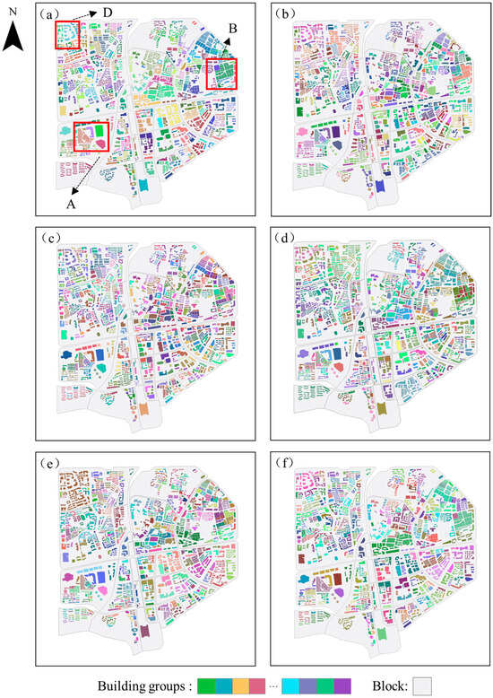
Figure 5.
Results of building grouping in Experimental Area I: (a) reference; (b) SCMC; (c) K-Means; (d) GCN; (e) the proposed method based solely on spatial geometric similarity; (f) the proposed method.
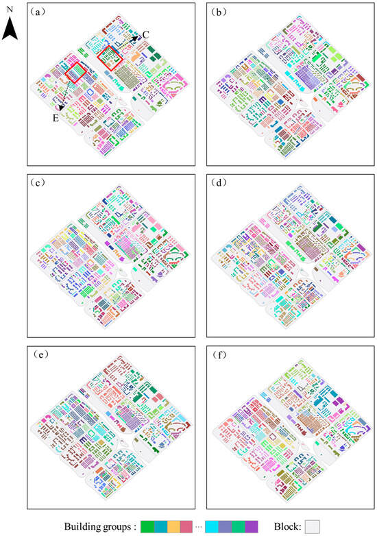
Figure 6.
Results of building grouping in Experimental Area II: (a) reference; (b) SCMC; (c) K-Means; (d) GCN; (e) the proposed method based solely on spatial geometric similarity; (f) the proposed method.
In contrast, while the SCMC and K-Means methods provide grouping results that are relatively close to the reference, discrepancies with the geographical reality are observed in certain areas. This is primarily due to the fact that these two methods consider both spatial geometric and semantic features during clustering, without first performing an initial grouping based on spatial geometry and then refining the classification based on semantic features. In areas with dense buildings and POIs, where building semantic features are highly similar, the SCMC and K-Means methods are easily influenced by semantic features, causing some buildings to be incorrectly grouped together solely due to semantic similarity, neglecting their differences in spatial geometry. Thus, clustering methods that directly merge spatial and semantic features may weaken the role of spatial geometry in certain cases, reducing the overall grouping validity.
Moreover, the GCN method performed poorly on the dataset used in this study. The primary reason for this is the insufficient number of samples in the dataset, which fails to provide enough training data for the GCN model, making it difficult for the model to learn sufficient generalizable features. The lack of enough samples also made the model overly sensitive to noise in the data, further affecting the accuracy of the grouping.
On the other hand, the proposed method, which relies solely on spatial geometric similarity for grouping, primarily depends on spatial geometric features such as building coordinates, size, shape, and orientation while not considering semantic features. This characteristic reveals significant drawbacks when applied to regions with complex building layouts or high semantic mixing. Due to the absence of semantic constraints, buildings might be erroneously grouped together simply based on similar spatial geometric features, leading to a significant decline in grouping quality. Furthermore, grouping methods that rely solely on spatial geometric features are highly sensitive to these features. For instance, in areas like residential communities, buildings often exhibit circular or other complex spatial arrangements. In such cases, traditional grouping methods driven by spatial geometric features often struggle to accurately identify these buildings as a distinct group, leading to grouping results that fail to meet the practical requirements of real-world applications.
To better illustrate the details of the method, we conducted an in-depth analysis at a smaller scale, selecting the representative regions A, B, C, D, and E. The specific geographic locations of these regions in the experimental areas are shown in Figure 5a and Figure 6a. We present the grouping references for these regions, the semantic labels of the buildings, the initial grouping results (based on the spatial geometric similarity constraint method described in Section 4.1), and the final building grouping results (using the complete method proposed in this paper), as shown in Figure 7, Figure 8, Figure 9, Figure 10 and Figure 11. In these figures, the red boxes highlight the specific buildings within each region that are the focus of our detailed analysis.
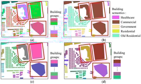
Figure 7.
Region A: (a) reference for building grouping; (b) semantic labeling of buildings; (c) initial building grouping results; (d) final building grouping results.
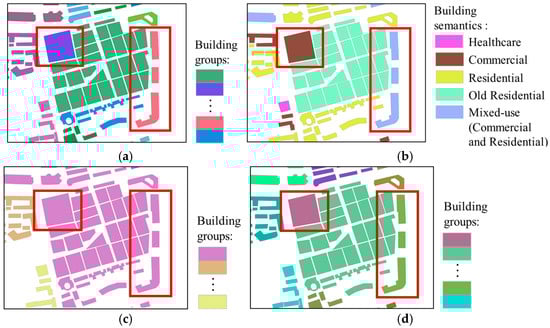
Figure 8.
Region B: (a) reference for building grouping; (b) semantic labeling of buildings; (c) initial building grouping results; (d) final building grouping results.
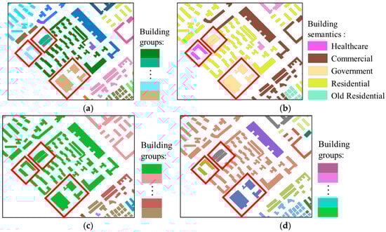
Figure 9.
Region C: (a) reference for building grouping; (b) semantic labeling of buildings; (c) initial building grouping results; (d) final building grouping results.
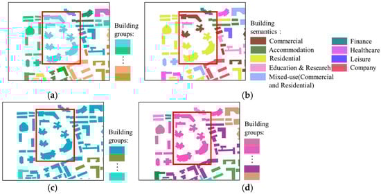
Figure 10.
Region D: (a) reference for building grouping; (b) semantic labeling of buildings; (c) initial building grouping results; (d) final building grouping results.
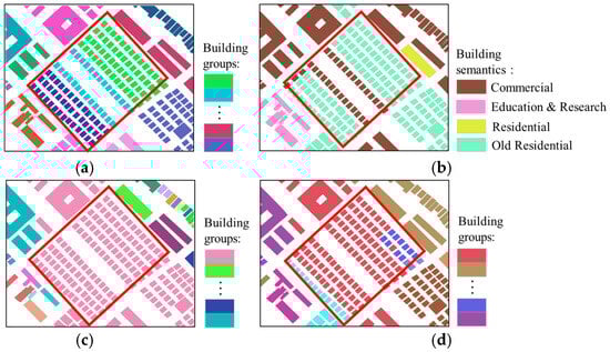
Figure 11.
Region E: (a) reference for building grouping; (b) semantic labeling of buildings; (c) initial building grouping results; (d) final building grouping results.
The details of Region A are shown in Figure 7. Region A mainly consists of regularly shaped old residential buildings and several commercial buildings with significantly different shapes. There are noticeable spatial geometric differences between the various building groups. Through the highlighted areas in Figure 7, it can be observed that when the buildings have similar semantic features but significant differences in spatial features, our method correctly classifies these buildings into three groups. This outcome is attributed to the spatial–semantic dual clustering strategy we proposed, which prioritizes spatial geometric features when grouping buildings, ensuring that the spatial relative positioning and geometric similarity between buildings are effectively preserved. Specifically, when buildings have significant differences in spatial distribution, even if their semantic features are similar, our method can still effectively distinguish them based on spatial geometric features.
The details of Region B are shown in Figure 8. The buildings in Region B are more densely distributed, and the spatial geometric differences between different building groups are relatively small. Observing the highlighted areas in Figure 8c, since these buildings are similar in shape and orientation to the surrounding buildings or are close in proximity, the initial grouping results of our method classify them into the same group, failing to distinguish them into different scenes accurately. However, after further incorporating semantic features, the highlighted area in Figure 8d shows that buildings with “commercial” semantics and “mixed-use” semantics are separately identified as two independent groups, distinct from other types of buildings. This result demonstrates that our method not only takes into account the spatial proximity between buildings but also fully incorporates their semantic feature differences, ensuring that buildings are precisely classified into their respective groups.
The details of Region C are shown in Figure 9. Region C is primarily composed of irregularly shaped residential buildings and buildings with relatively scarce semantic categories. Observing the highlighted areas in Figure 9d, buildings with “government” and “healthcare” semantics are separately identified and classified into two independent groups. Although the number of POIs reflecting these two semantic features is relatively small, the TF–IDF method is still able to effectively identify and extract the semantic features of the buildings, achieving accurate classification. This demonstrates that even when dealing with buildings with relatively scarce semantic categories, the identification and grouping based on semantic similarity can still be efficiently accomplished.
However, although the method performs excellently in most cases, there are still some failure cases in certain special situations. As shown in Figure 10 and Figure 11, some buildings with consistent spatial and semantic features were not successfully identified and grouped. For example, in Figure 10, buildings with similar spatial features but different semantic features were mistakenly grouped together. The primary reason for this is the high density of buildings and the low POI density. The high building density causes these buildings to be influenced by the same POIs when identifying their semantic features, thus reducing the distinguishability of their semantic characteristics. Furthermore, due to the low POI density, some building outlines lack POI data internally, and without strongly correlated POIs to assist in identifying their semantic features, they are more likely to be influenced by nearby POIs, leading to reduced accuracy in semantic feature recognition. In Figure 11, buildings with low proximity are sometimes incorrectly grouped together, indicating that the method failed to correctly group the buildings during the building division based on spatial geometric similarity constraints. The root cause of this issue is closely related to the stopping criteria in the initial clustering process based on spatial similarity. Although an adaptive strategy (i.e., the introduction of adjustment parameter ) was applied, determining how to set parameters to accommodate the diverse clustering needs of buildings across different neighborhoods remains a significant challenge.
5.3. Quality Evaluation
Currently, various building grouping quality evaluation methods have been proposed, which can generally be divided into two categories: unsupervised and supervised methods []. Supervised clustering evaluation methods directly assess the accuracy of grouping results based on predefined correct groupings or “truth value” labels. By utilizing label information, supervised methods can align more closely with human cognitive patterns, providing a more detailed evaluation of the grouping results and thus more effectively reflecting the reasonableness of building groupings. The Adjusted Rand Index (ARI) is a supervised clustering evaluation method that assesses clustering validity by calculating the number of sample pairs assigned to the same or different clusters in both the predefined labels and the clustering results []. Therefore, we selected the ARI as the evaluation metric to assess the quality of building grouping results. Let and denote the predicted clusters and predefined labels of buildings in a region, respectively. The ARI is calculated as follows:
where is the number of buildings common to both and , is the number of buildings in , is the number of buildings in , and is the total number of buildings. ARI is a dimensionless metric, with a range of , where higher values indicate better grouping performance.
We conducted a statistical evaluation of the grouping performance of different methods using the ARI. Figure 12 and Figure 13 summarize the ARI values for the proposed method with optimal parameters and the comparative methods under different parameter settings, including their best ARI results. It should be noted that the proposed method based solely on spatial geometric similarity, the complete proposed method, SCMC, and K-Means methods all calculate ARI based on all buildings in the two experiment areas, while the GCN method, due to the 7:3 split of the dataset into training and test sets, calculates its ARI value only based on the test set.
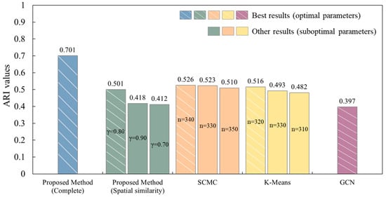
Figure 12.
Comparison of ARI values in Experimental Area I: proposed method (optimal parameters) vs. comparative methods (varying parameters), where n denotes the number of clusters, and denotes the adjustment parameter.
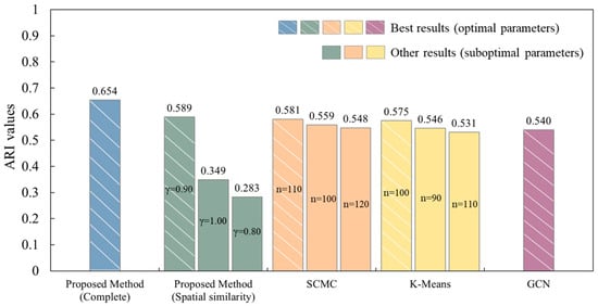
Figure 13.
Comparison of ARI values in Experimental Area II: proposed method (optimal parameters) vs. comparative methods (varying parameters), where n denotes the number of clusters, and denotes the adjustment parameter.
The results show that the proposed method achieved the highest ARI values in both datasets, 0.701 and 0.654, demonstrating the best performance. Furthermore, the results based solely on spatial geometric similarity grouping (0.501 and 0.589) show that spatial geometric features play an important role in building grouping tasks, but using this feature alone is not enough to achieve optimal performance, further validating the key role of semantic features in building grouping. For the SCMC and K-Means methods, the ARI values in test areas I and II are 0.526 and 0.581 and 0.516 and 0.575, respectively. In Experimental Area II, the best ARI values of these two methods are slightly lower than those of the proposed method based solely on spatial geometric similarity, while in Experimental Area I, their best ARI values are slightly higher. However, overall, these methods still perform significantly worse than the full proposed method. This suggests that traditional methods have certain limitations when dealing with complex data. The best ARI values for the GCN method are relatively low (0.397 and 0.540), primarily due to the small sample size of the dataset, which did not provide sufficient training data for the GCN model, affecting its grouping performance. This result indicates that although GCN has strong feature learning capabilities, its generalization ability is limited when the data scale is small.
5.4. Parameter Sensitivity Analysis
To explore the parameter sensitivity of our method, we conducted experiments by varying key parameters, including the weights in the formula for the overall spatial geometric similarity, the adjustment parameter in the definition of spatial geometric feature homogeneity, and the semantic similarity threshold in the definition of semantic similarity.
Firstly, we tested the four weights in the formula for the overall spatial geometric similarity. Specifically, we ensured that the weights representing the similarity in the geometric form of buildings—namely, size, shape, and orientation similarity—were balanced with the weight assigned to the proximity index, which reflects the spatial proximity of buildings. To achieve this, we set the weight for the proximity index to 0.5, and the sum of the remaining weights was also 0.5. Based on this configuration, we conducted experiments using the building data from Experimental Area I and II, following the methodology outlined in Section 4.1, while keeping the adjustment parameter constant. The results revealed that while variations in the weight combinations did influence the ARI values, the differences were not significant. For instance, the combination [0.5, 0.2, 0.2, 0.1] resulted in the highest ARI value of 0.534, while the combination [0.5, 0.2, 0.1, 0.2] produced the lowest ARI value of 0.503.
Furthermore, using the complete proposed method, we investigated the impact of the adjustment parameter and the semantic similarity threshold on the building grouping results. Specifically, we conducted detailed experiments while fixing the weight combination of the overall spatial geometric similarity formula as [0.5, 0.2, 0.2, 0.1] to determine the optimal parameter configuration for the two experimental areas. The experimental results are shown in Table 3 and Table 4.
Table 3.
ARI values of the proposed method under different parameters in Experimental Area I.
Table 4.
ARI values of the proposed method under different parameters in Experimental Area II.
The experimental results show that as the adjustment parameter increases, the accuracy of the building grouping results initially increases and then decreases. This behavior can be attributed to the fact that the adjustment parameter determines the granularity of the grouping based on spatial geometric similarity constraints: when is large, the grouping criteria become more relaxed, making it difficult to distinguish buildings with different spatial geometric features; when is small, the grouping granularity becomes too fine, which may prevent the subsequent clustering based on semantic similarity from aggregating similar groups, thus affecting the grouping results.
Additionally, the variation in the semantic similarity threshold also significantly influences the grouping results. As increases, the accuracy of the building grouping results shows a trend of first increasing and then decreasing. Under the condition of the adjustment parameter , the grouping results in Experimental Area I achieve the highest accuracy when ; under the condition of , the best performance in Experimental Area II is observed when . This suggests that the proper setting of the semantic similarity threshold is crucial to ensure the accuracy of semantic feature clustering.
6. Discussion
The performance of the proposed method in the building grouping task is significantly affected by the quality and quantity of POI data within the experimental areas. To further explore this issue, we compared the proportions of different POI categories in the two experimental areas and analyzed how the distribution of POI data influences the grouping accuracy of buildings, combined with the ARI values of buildings with different semantic features. Experimental Area I is located in the southern part of Shenzhen, where buildings are primarily categorized as commercial, financial, and old residential; Experimental Area II is located in the western part of Shenzhen, away from the city center, with buildings mainly categorized as residential and old residential.
As shown in Figure 14, the proportion of Life and Dining POIs accounts for more than 60% of the total POIs in both experimental areas. When excluding these two types of POIs, it can be observed that in Experimental Area I, the proportions of residential, finance, accommodation, and leisure POIs are close to each other, with no dominant type, resulting in a relatively balanced POI distribution. This provides richer semantic support, helping the algorithm more accurately identify building clusters. In contrast, Experimental Area II shows a more skewed POI distribution, with a higher proportion of residential POIs and lower proportions of other categories. Moreover, the general lack of residential POIs in the dataset is a significant drawback as it results in many buildings in Experimental Area II lacking sufficient semantic support, which leads to a decrease in grouping accuracy.
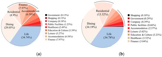
Figure 14.
Proportion of different types of POIs: (a) Experimental Area I; (b) Experimental Area II.
Figure 15 further illustrates the ARI values of building grouping results for different semantic categories. The results show that the grouping performance of transportation, leisure, financial, and government buildings is relatively excellent, with ARI values close to or exceeding 0.9, indicating that these categories have prominent semantic features and high grouping accuracy. In contrast, although residential and old residential buildings are more numerous, the grouping performance of some of them is relatively poor. In Experimental Areas I and II, the ARI values for residential buildings are 0.479 and 0.527, respectively, and the ARI value for old residential buildings in Experimental Area II is 0.569. The reason for this phenomenon lies in the fact that the grouping of residential buildings is highly dependent on residential POI data, which often suffers from missing data, directly causing fluctuations in grouping accuracy: when residential POI data are complete, grouping accuracy is high, but when POI data are missing, grouping accuracy significantly decreases. Moreover, old residential buildings also lack residential POI support, and the POI types around them are more complex, potentially including leisure, commercial, and other categories, which causes semantic confusion and increases the difficulty of grouping. The grouping of company buildings in Experimental Area II shows the worst performance, with an ARI value of only 0.143, mainly due to the small sample size of company buildings (only 6), with the insufficient sample size exacerbating the uncertainty of the grouping results.
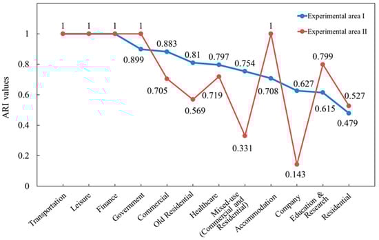
Figure 15.
ARI values of different semantic building groups.
Overall, the quantity and quality of POI data play a decisive role in the accuracy of building grouping. In areas with more complete POI data, the algorithm can better combine spatial and semantic information for grouping, whereas in areas with sparse or singularly distributed POI data, the semantic features of buildings are difficult to fully represent, leading to lower grouping accuracy.
7. Conclusions
This paper addresses the insufficient attention to building semantic features in current grouping research and proposes a method that combines spatial geometric and semantic features for building grouping. The method utilizes spatial geometric and functional semantic information from multi-source ubiquitous data for feature representation. It adopts a spatial–semantic dual clustering strategy and integrates optimization-based graph segmentation to refine the grouping results, thereby identifying building groups that align with human geographic spatial cognition. To validate the effectiveness of the method, two distinct areas in the Luohu and Baoan districts of Shenzhen were selected for experimentation. The experimental results demonstrate that the proposed method outperforms the SCMC methods, K-Means clustering, the graph deep-learning-based method, and the spatial geometric similarity-based method in building grouping tasks and can accurately identify building groups that are spatially proximate and semantically similar.
However, due to variations in the quality and distribution of POI data across regions, particularly in areas with scarce POI data, the complete representation of building semantic features is limited, which in turn affects grouping accuracy. Therefore, future research could introduce richer and more accurate sources of semantic data, such as social media and taxi trajectory data, to mitigate the limitations of POI data. Furthermore, integrating multimodal data fusion with deep learning techniques in future studies will enable more precise identification of complex relationships between buildings, thus advancing the development of intelligent and personalized map-making and knowledge services in the era of big data.
Author Contributions
Conceptualization, Huimin Liu, Wenpei Wang, and Chen Ding; Data Curation, Huimin Liu and Wenpei Wang; Formal Analysis, Wenpei Wang; Funding Acquisition, Huimin Liu, Jianbo Tang, and Min Deng; Investigation, Huimin Liu and Wenpei Wang; Methodology, Huimin Liu, Wenpei Wang, and Jianbo Tang; Project Administration, Huimin Liu; Resources, Huimin Liu; Software, Wenpei Wang; Supervision, Huimin Liu, Jianbo Tang, Min Deng, and Chen Ding; Validation, Wenpei Wang; Visualization, Huimin Liu; Writing—Original Draft, Huimin Liu and Wenpei Wang; Writing—Review and Editing, Huimin Liu and Chen Ding. All authors have read and agreed to the published version of the manuscript.
Funding
This research was funded by the National Natural Science Foundation of China, grant numbers 42430110, 42471487, 42271462, and 42171441, the Funds of the Science and Technology Innovation Program of Hunan Province, grant number 2024AQ2026, the Hunan Provincial Natural Science Foundation of China, grant numbers 2025JJ20038, 2024JJ1009, and 2024JJ8343, the Funds of Open Projects of Hunan Geospatial Information Engineering and Technology Research Center, grant number HNGIET2024002, the Funds of Open Projects of Hunan Engineering Research Center of Geographic information security and application, grant number HNGISA2024001, the Graduate Innovation Project of Central South University, grant number 2022XQLH099, and the Fundamental Research Funds for the Central Universities of Central South University, grant number 2024ZZTS0055.
Data Availability Statement
Dataset available on request from the authors. The data are not publicly available due to the fact that they contain data that are subject to further research.
Conflicts of Interest
The authors declare no conflicts of interest.
References
- Li, Z. Digital Map Generalization at the Age of Enlightenment: A Review of the First Forty Years. Cartogr. J. 2007, 44, 80–93. [Google Scholar] [CrossRef]
- Yu, W.; Chen, Y. Data-Driven Polyline Simplification Using a Stacked Autoencoder-Based Deep Neural Network. Trans. GIS 2022, 26, 2302–2325. [Google Scholar] [CrossRef]
- He, X.; Zhang, X.; Xin, Q. Recognition of Building Group Patterns in Topographic Maps Based on Graph Partitioning and Random Forest. ISPRS J. Photogramm. Remote Sens. 2018, 136, 26–40. [Google Scholar] [CrossRef]
- Herold, M.; Couclelis, H.; Clarke, K.C. The Role of Spatial Metrics in the Analysis and Modeling of Urban Land Use Change. Comput. Environ. Urban Syst. 2005, 29, 369–399. [Google Scholar] [CrossRef]
- Xing, R.; Wu, F.; Gong, X.; Du, J.; Liu, C. An Axis-Matching Approach to Combined Collinear Pattern Recognition for Urban Building Groups. Geocarto Int. 2022, 37, 4823–4842. [Google Scholar] [CrossRef]
- Hu, Y.; Liu, C.; Li, Z.; Xu, J.; Han, Z.; Guo, J. Few-Shot Building Footprint Shape Classification with Relation Network. ISPRS Int. J. Geo-Inf. 2022, 11, 311. [Google Scholar] [CrossRef]
- Du, S.; Shu, M.; Feng, C.-C. Representation and Discovery of Building Patterns: A Three-Level Relational Approach. Int. J. Geogr. Inf. Sci. 2016, 30, 1161–1186. [Google Scholar] [CrossRef]
- Yu, W.; Ai, T.; Liu, P.; Cheng, X. The Analysis and Measurement of Building Patterns Using Texton Co-Occurrence Matrices. Int. J. Geogr. Inf. Sci. 2017, 31, 1079–1100. [Google Scholar] [CrossRef]
- He, X.; Deng, M.; Luo, G. Recognizing Building Group Patterns in Topographic Maps by Integrating Building Functional and Geometric Information. ISPRS Int. J. Geo-Inf. 2022, 11, 332. [Google Scholar] [CrossRef]
- Deng, M.; Tang, J.; Liu, Q.; Wu, F. Recognizing Building Groups for Generalization: A Comparative Study. Cartogr. Geogr. Inf. Sci. 2018, 45, 187–204. [Google Scholar] [CrossRef]
- Wang, X.; Burghardt, D. A Mesh-Based Typification Method for Building Groups with Grid Patterns. ISPRS Int. J. Geo-Inf. 2019, 8, 168. [Google Scholar] [CrossRef]
- Wei, Z.; Ding, S.; Cheng, L.; Xu, W.; Wang, Y.; Zhang, L. Linear Building Pattern Recognition in Topographical Maps Combining Convex Polygon Decomposition. Geocarto Int. 2022, 37, 11365–11389. [Google Scholar] [CrossRef]
- Yang, M.; Yuan, T.; Yan, X.; Ai, T.; Jiang, C. A Hybrid Approach to Building Simplification with an Evaluator from a Backpropagation Neural Network. Int. J. Geogr. Inf. Sci. 2022, 36, 280–309. [Google Scholar] [CrossRef]
- Qi, H.B.; Li, Z.L. An Approach to Building Grouping Based on Hierarchical Constraints. Int. Arch. Photogramm. Remote Sens. Spatial Inf. Sci. 2008, 2008, 449–454. [Google Scholar]
- Regnauld, N. Contextual Building Typification in Automated Map Generalization. Algorithmica 2001, 30, 312–333. [Google Scholar] [CrossRef]
- Zhang, X.; Ai, T.; Stoter, J.; Kraak, M.-J.; Molenaar, M. Building Pattern Recognition in Topographic Data: Examples on Collinear and Curvilinear Alignments. Geoinformatica 2013, 17, 1–33. [Google Scholar] [CrossRef]
- Zhang, F.; Sun, Q.; Ma, J.; Lyu, Z.; Huang, Z. A Polygonal Buildings Aggregation Method Considering Obstacle Elements and Visual Clarity. Geocarto Int. 2023, 38, 2266672. [Google Scholar] [CrossRef]
- Liu, P.; Shao, Z.; Xiao, T. Second-Order Texton Feature Extraction and Pattern Recognition of Building Polygon Cluster Using CNN Network. Int. J. Appl. Earth Obs. Geoinf. 2024, 129, 103794. [Google Scholar] [CrossRef]
- Wei, Z.; Guo, Q.; Wang, L.; Yan, F. On the Spatial Distribution of Buildings for Map Generalization. Cartogr. Geogr. Inf. Sci. 2018, 45, 539–555. [Google Scholar] [CrossRef]
- Yan, X.; Ai, T.; Yang, M.; Tong, X. Graph Convolutional Autoencoder Model for the Shape Coding and Cognition of Buildings in Maps. Int. J. Geogr. Inf. Sci. 2021, 35, 490–512. [Google Scholar] [CrossRef]
- Basaraner, M.; Cetinkaya, S. Performance of Shape Indices and Classification Schemes for Characterising Perceptual Shape Complexity of Building Footprints in GIS. Int. J. Geogr. Inf. Sci. 2017, 31, 1952–1977. [Google Scholar] [CrossRef]
- Ma, W.; Wang, B.; Liu, C.; Li, Q.; Yang, C.; Pan, J.; Zhou, B.; Wang, Y. Complex Buildings Orientation Recognition and Description Based on Vector Reconstruction. Int. J. Appl. Earth Obs. Geoinf. 2023, 123, 103486. [Google Scholar] [CrossRef]
- Hangouët, J.F.; Müller, J.C. Approche et Méthodes Pour l’automatisation de La Généralisation Cartographique; Application En Bord de Ville. Ph.D. Thesis, Université de Marne La Vallée, Paris, France, 1999. [Google Scholar]
- Yan, H.; Weibel, R.; Yang, B. A Multi-Parameter Approach to Automated Building Grouping and Generalization. Geoinformatica 2008, 12, 73–89. [Google Scholar] [CrossRef]
- Yan, X.; Ai, T.; Yang, M.; Tong, X.; Liu, Q. A Graph Deep Learning Approach for Urban Building Grouping. Geocarto Int. 2022, 37, 2944–2966. [Google Scholar] [CrossRef]
- Wang, W.; Du, S.; Guo, Z.; Luo, L. Polygonal Clustering Analysis Using Multilevel Graph-Partition. Trans. GIS 2015, 19, 716–736. [Google Scholar] [CrossRef]
- Yan, X.; Ai, T.; Yang, M.; Yin, H. A Graph Convolutional Neural Network for Classification of Building Patterns Using Spatial Vector Data. ISPRS J. Photogramm. Remote Sens. 2019, 150, 259–273. [Google Scholar] [CrossRef]
- Zhao, R.; Ai, T.; Yu, W.; He, Y.; Shen, Y. Recognition of Building Group Patterns Using Graph Convolutional Network. Cartogr. Geogr. Inf. Sci. 2020, 47, 400–417. [Google Scholar] [CrossRef]
- Wang, X.; Burghardt, D. Using Stroke and Mesh to Recognize Building Group Patterns. Int. J. Cartogr. 2020, 6, 71–98. [Google Scholar] [CrossRef]
- Toussaint, G.T.; Bhattacharya, B.K. Optimal Algorithms for Computing the Minimum Distance between Two Finite Planar Sets. Pattern Recognit. Lett. 1983, 2, 79–82. [Google Scholar] [CrossRef]
- Wang, J.; Luo, H.; Li, W.; Huang, B. Building Function Mapping Using Multisource Geospatial Big Data: A Case Study in Shenzhen, China. Remote Sens. 2021, 13, 4751. [Google Scholar] [CrossRef]
- Psyllidis, A.; Gao, S.; Hu, Y.; Kim, E.-K.; McKenzie, G.; Purves, R.; Yuan, M.; Andris, C. Points of Interest (POI): A Commentary on the State of the Art, Challenges, and Prospects for the Future. Comput. Urban Sci. 2022, 2, 20. [Google Scholar] [CrossRef] [PubMed]
- Deng, Y.; Chen, R.; Yang, J.; Li, Y.; Jiang, H.; Liao, W.; Sun, M. Identify Urban Building Functions with Multisource Data: A Case Study in Guangzhou, China. Int. J. Geogr. Inf. Sci. 2022, 36, 2060–2085. [Google Scholar] [CrossRef]
- Cao, Y.; Liu, J.; Wang, Y.; Wang, L.; Wu, W.; Su, F. A Study on the Method for Functional Classification of Urban Buildings by Using POI Data. J. Geo Inf. Sci. 2020, 22, 1339–1348. [Google Scholar] [CrossRef]
- Salton, G.; McGill, M. Introduction to Modern Information Retrieval; McGraw-Hill: New York, NY, USA, 1 September 1983. [Google Scholar]
- Salton, G.; Buckley, C. Term-Weighting Approaches in Automatic Text Retrieval. Inf. Process. Manag. 1988, 24, 513–523. [Google Scholar] [CrossRef]
- Choi, K.; Suh, Y. A New Similarity Function for Selecting Neighbors for Each Target Item in Collaborative Filtering. Knowl. Based Syst. 2013, 37, 146–153. [Google Scholar] [CrossRef]
- Chrisochoides, N.; Sukup, F. Task Parallel Implementation of the Bowyer-Watson Algorithm; Advanced Computing Research Institue cornell University: Ithaca, NY, USA, 1 February 1996. [Google Scholar]
- Prim, R.C. Shortest Connection Networks And Some Generalizations. Bell Syst. Tech. J. 1957, 36, 1389–1401. [Google Scholar] [CrossRef]
- Calinski, T.; Harabasz, J. A Dendrite Method for Cluster Analysis. Comm. Stats. Theory Methods 1974, 3, 1–27. [Google Scholar] [CrossRef]
- AssunÇão, R.M.; Neves, M.C.; Câmara, G.; Da Costa Freitas, C. Efficient Regionalization Techniques for Socio-economic Geographical Units Using Minimum Spanning Trees. Int. J. Geogr. Inf. Sci. 2006, 20, 797–811. [Google Scholar] [CrossRef]
- MacQueen, J.B. Some Methods for Classification and Analysis of Multivariate Observations; University of California Press: Berkeley, CA, USA, 1967. [Google Scholar]
- Kipf, T.N.; Welling, M. Semi-Supervised Classification with Graph Convolutional Networks. arXiv 2016, arXiv:1609.02907. [Google Scholar]
- Jiang, B. Spatial Clustering for Mining Knowledge in Support of Generalization Processes in GIS. Available online: https://www.semanticscholar.org/paper/Spatial-Clustering-for-Mining-Knowledge-in-Support-Jiang/6256915c5d224dcf618cc92afe55b8b06f7e2663 (accessed on 1 March 2024).
- Touya, G.; Zhang, X.; Lokhat, I. Is Deep Learning the New Agent for Map Generalization? Int. J. Cartogr. 2019, 5, 142–157. [Google Scholar] [CrossRef]
- Hubert, L.; Arabie, P. Comparing Partitions. J. Classif. 1985, 2, 193–218. [Google Scholar] [CrossRef]
Disclaimer/Publisher’s Note: The statements, opinions and data contained in all publications are solely those of the individual author(s) and contributor(s) and not of MDPI and/or the editor(s). MDPI and/or the editor(s) disclaim responsibility for any injury to people or property resulting from any ideas, methods, instructions or products referred to in the content. |
© 2025 by the authors. Published by MDPI on behalf of the International Society for Photogrammetry and Remote Sensing. Licensee MDPI, Basel, Switzerland. This article is an open access article distributed under the terms and conditions of the Creative Commons Attribution (CC BY) license (https://creativecommons.org/licenses/by/4.0/).