Evaluating Shallow Landslide Prediction Mapping by Using Two Different GIS-Based Models: 4SLIDE and SHALSTAB

Abstract

Landslides affecting soil layers up to 1–2 m deep pose a significant hazard in mountainous and hilly regions, particularly in the Mediterranean, where intense precipitation is increasing. Identifying landslide-prone areas is crucial for risk assessment and mitigation, as landslides can severely impact land surfaces, infrastructure, and inhabited areas. Forest cover and management play a fundamental role in stabilizing soil and reducing landslide susceptibility. This study focuses on landslide forecasting models, which integrate geological, climatic, and topographic data to predict landslide probability and severity. Specifically, we compare the predictive accuracy of the 4SLIDE model with the established SHALSTAB model in a forested mountain catchment within Sila National Park, Southern Italy, using GIS-based analysis. The results demonstrate that both models effectively identify high-risk areas, with ROC analysis confirming the superior predictive capability of the 4SLIDE model. Our findings underscore the critical importance of early landslide identification, supporting timely interventions and the implementation of forest engineering and Civil Protection measures to mitigate the impact of landslides on communities and infrastructure.

1. Introduction

Landslide susceptibility indicates the likelihood that a particular area will experience landslides or soil slippage. This susceptibility is shaped by various factors, including geological, environmental, and human-related influences [1]. Landslide susceptibility depends on factors such as topography (steep slopes), soil type (clayey/silty), and intense rainfall, which saturates the soil. These factors increase the risk of landslides and mudflows [2,3,4]. Human activities (like construction or deforestation) and past landslides increase regional vulnerability [1,3]. Risk assessment, through geotechnical and hydrological analyses, allows the identification of critical areas and the planning of interventions (engineering structures, soil stabilization, or monitoring) [5,6]. Natural disasters such as landslides, cause fatalities, but preventive measures and rapid responses can reduce them. Landslide hazard refers to the potential for slope failure, while risk quantifies the resulting economic and human losses [5]. Landslides are the result of a combination of natural factors (like heavy rainfall or floods) and human factors (like land use changes or deforestation) [7,8]. The interaction between rain, surface runoff, and subsurface runoff destabilizes slopes by eroding materials and modifying the regolith. Deforestation, hill cutting, and inadequate rural land planning, which represent forms of poor land management, are primary causes that exacerbate triggering factors and increase landslide risk [9,10]. According to the United Nations Office for Disaster Risk Reduction (UNDRR), landslides accounted for approximately 5% of all natural disaster-related deaths between 1998 and 2017, with over 18,000 fatalities globally [11]. Natural disasters in 2016 caused 8733 deaths and $154 billion in damages, highlighting the devastating socio-economic impact of these events [11]. Italy is among the most vulnerable European countries in this regard, with 620,808 landslides affecting 23,700 km², or 7.9% of its national territory [12,13,14]. Vegetation cover plays a crucial role in reducing hydrogeological risks, preventing runoff and surface erosion, and increasing soil shear resistance through root systems [5,15]. One of the key approaches for developing risk reduction strategies is the creation of a landslide susceptibility map (LSM). An LSM offers a spatial distribution of potential landslides, thus playing an essential role in mitigating landslide risk [16]. Models estimate risks and generate probability maps under various forest management and rainfall scenarios. Models for predicting landslide susceptibility are crucial tools for managing and mitigating natural risks [5]. These models help identify areas potentially prone to landslides, allowing planners and decision-makers to take preventive measures and reducing the impact of such events on people, infrastructure, and the environment [17]. Various methods for generating landslide susceptibility maps have been demonstrated over the past decades [5,15,18,19,20]. Landslide susceptibility mapping models offer several benefits, such as risk prevention and mitigation by identifying at-risk areas for planning interventions, emergency management by locating hazardous areas during critical events, land planning by supporting urban development and environmental conservation, and environmental monitoring by assessing the impact of climatic and environmental changes. Many researchers have explored different approaches for creating LSMs. In addition to crisis management, LSMs are crucial for identifying areas at risk of landslides, as well as for managing and reducing such risks [21]. These maps can be generated using an appropriate model, incorporating landslide data and a set of independent variables [22]. There are three main groups of landslide susceptibility methods: innovative, deterministic, and statistical [23]. Innovative models rely on expert judgment to assign weights to each factor. Therefore, this type of model has a higher potential for errors [24]. Deterministic models are developed based on mathematical relationships. These models are grounded in physical laws, requiring the calculation of the relationship between resisting forces and the drivers of mass movements [25].

4SLIDE is a physical model based on a deterministic approach, used to simulate slope stability and predict susceptibility to shallow landslides [19]. The 4SLIDE model integrates geological, topographical, and hydrological parameters to estimate a Factor of Safety (FS) index, indicating the stability of a location (0 represents the most unstable state, while 1.5 represents the most stable state). SHALSTAB (Shallow Landsliding Stability Model) is another widely used physical-deterministic model for predicting shallow landslides. It relies on analyzing slope stability alongside a hydrological model to assess soil saturation levels from rainfall and the potential for shallow landslides [26]. 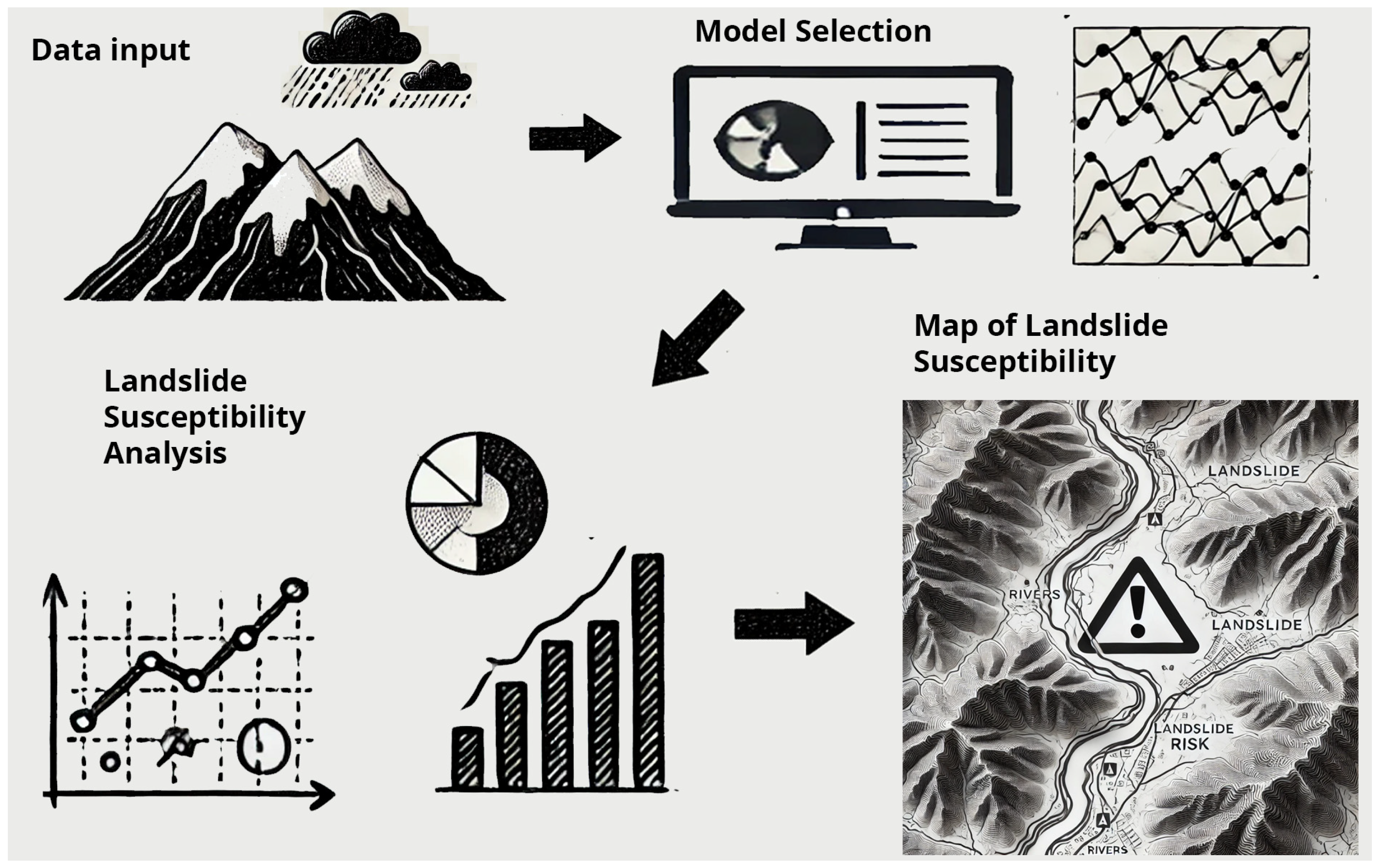Both SHALSTAB and 4SLIDE are powerful tools in landslide risk management, each suited to specific contexts (Figure 1). SHALSTAB is ideal for large-scale analyses, especially in high-rainfall regions, where it predicts risk effectively over broad areas. In contrast, 4SLIDE is tailored for detailed site-specific analysis, especially in locations where soil characteristics are crucial to understanding risk. Both models utilize numerical geotechnical parameters distributed spatially within a raster-based GIS framework. However, their integration enables a more comprehensive and detailed understanding of the dynamics of landslide susceptibility. Comparing landslide susceptibility models not only helps assess the robustness and reliability of predictions but also identifies differences and similarities between the two approaches, thereby enhancing the accuracy of risk estimates. This dual analysis allows for the combination of the strengths of both models, enabling the identification of the most appropriate one for specific scenarios and, in some cases, suggesting their integrated use.

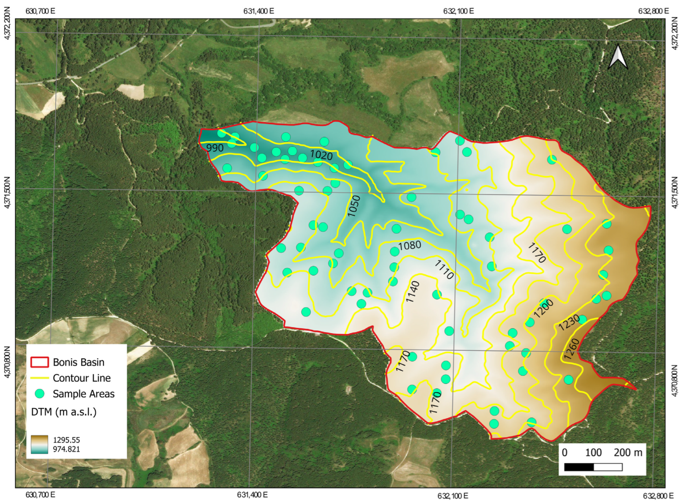
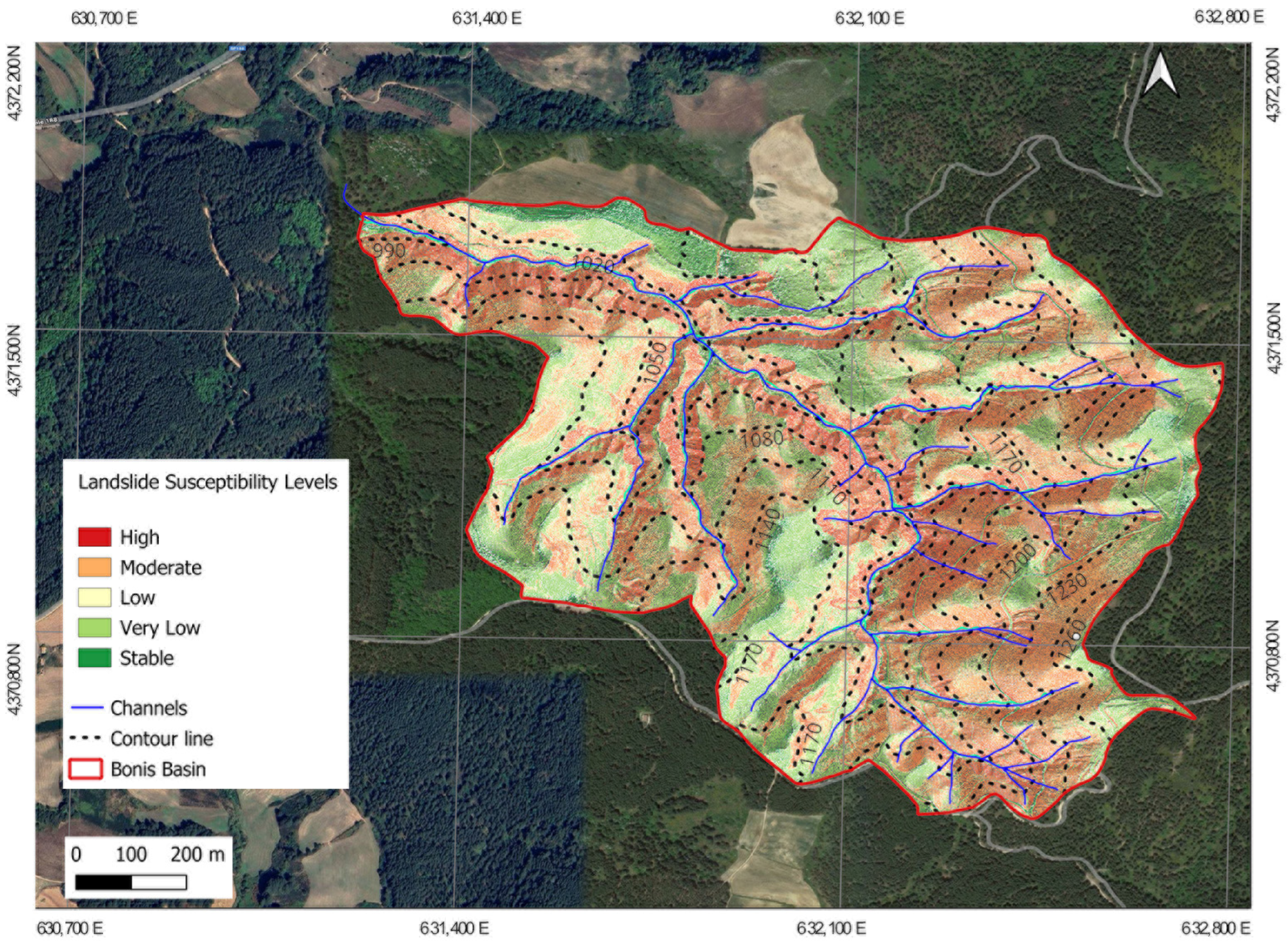
This study compares the 4SLIDE model with another landslide susceptibility mapping model, SHALSTAB, highlighting the innovation of an in-depth comparative analysis based on the combined use of two distinct modeling approaches. For a comparative analysis of the different parameter percentages in landslide-prone areas, such as susceptibility assessments provided by models like 4SLIDE or SHALSTAB, it is useful to examine the distribution of various risk categories (e.g., low, medium, and high) over a specific map or region. This approach may include comparing the percentages of different risk levels or analyzing variations in a key parameter, such as terrain slope or soil saturation, within distinct risk zones. The novelty of the study lies in the direct comparison between the two models, which represent complementary but distinct methodologies. Focusing on detailed geotechnical analysis, 4SLIDE considers physical parameters of the terrain, such as slope stability and sliding phenomena, with high local resolution. On the other hand, SHALSTAB adopts a more generalized hydrological approach, based on hydrological thresholds and a broader scale of analysis, suitable for estimating risk areas in regional contexts. This process represents a methodological innovation that not only supports decision-making in risk management and landslide prevention planning but also makes a significant contribution to improving the practical applicability and reliability of existing models, ensuring more effective and sustainable land management. The comparison of the two models was conducted in data from the Bonis catchment, an experimental forested area in Calabria, southern Italy, which serves as an ideal research site for studying hydrology, meteorology, and forestry in a Mediterranean mountain environment. This catchment features varied topography, including steep slopes, diverse soil types, and vegetation. Thus, it reflects the complexities of landslide-prone regions. Equipped with an advanced monitoring network, the Bonis catchment tracks geotechnical and hydrological parameters, such as surface runoff, groundwater levels, soil moisture, and precipitation, providing high-resolution data essential for model calibration and validation [27]. The catchment’s small size and consistent land use minimize external influences, offering a controlled environment for focused analysis of landslide susceptibility factors like soil properties, slope stability, and hydrology. Overall, the Bonis catchment is a representative site for evaluating landslide susceptibility models in Mediterranean mountain regions, making it an ideal location for this comparative study [27].

2. Materials and Methods

2.1. The 4SLIDE Model

4SLIDE is a GIS-implemented toolbox for ArcGIS© 10.3 (and later versions), a comprehensive geographic information system developed by ESRI as closed-source software. In contrast, the 4SLIDE model is an open-source .tbx file that can be easily imported as an external toolbox within ArcMap [19]. This model integrates the infinite slope stability equation [28] with the hydrological model “TOPMODEL” [29] to compute the Factor of Safety Index, assessing landslide risk at the catchment scale. The model also incorporates the soil reinforcement effect via a vegetation root strength model, following the principles established by Wu [30]. It focuses on the analysis of landslide bodies with well-defined sliding surfaces, often circular or planar in shape. The software provides a detailed analysis of internal soil forces and the interactions between the different geological layers present in the slope [19,28]. In particular, 4SLIDE allows an in-depth analysis of the effect of the water table on slope stability. This includes evaluating the contribution of pore water pressures and drainage conditions, providing a more accurate representation of the site’s hydrogeological conditions [29]. The Factor of Safety (FS) is determined by the following formula:

$$FS={\displaystyle \frac{{\mathit{c}}_{\mathit{r}}+{\mathit{c}}_{\mathit{s}}+\left({\mathit{\rho }}_{\mathit{s}}\ast \mathit{g}\ast \mathit{z}\ast {\mathit{c}\mathit{o}\mathit{s}}^{\mathbf{2}}\mathit{\theta }-{\mathit{\rho }}_{\mathit{w}}\ast \mathit{g}\ast \mathit{h}{\mathit{c}\mathit{o}\mathit{s}}^{\mathbf{2}}\mathit{\theta }\right)\ast \mathit{t}\mathit{a}\mathit{n}\mathit{\varnothing }}{{\mathit{\rho }}_{\mathit{s}}\ast \mathit{g}\ast \mathit{z}\ast \mathit{s}\mathit{i}\mathit{n}\mathit{\theta }\ast \mathit{c}\mathit{o}\mathit{s}\mathit{\theta }}}$$

(1)

The wet soil density, denoted as ρ_s (kg/m³), represents the soil weight, including its moisture content. Another important parameter is the soil depth, indicated by z and measured in meters (m). The slope angle of the terrain is given by θ and is measured in degrees. Next, we have the water density, ρ_w, also expressed in kilograms per cubic meter (kg/m³), which represents how heavy the water is per unit of volume. The water level, denoted by h, is measured in meters (m). Soil and plant roots enhance slope stability by providing additional cohesion. The cohesion due to the roots is denoted by c_r, while the cohesion provided by the soil is denoted by c_s. Both cohesive forces are measured in Newtons per square meter (N/m²). Finally, gravity, denoted as g and measured in meters per second squared (m/s²), represents the acceleration due to the gravitational force acting on all these elements. The use of wet soil density in the equation reflects its similarity to field conditions during landslide initiation. FS values have specific meanings: an FS of 1 indicates a critical equilibrium state, suggesting imminent failure, an FS below 1 signals slope collapse, and an FS above 1.5 indicates stability [5,7]. The model’s output is a “soil stability map”, a raster representation of the Factor of Safety (FS). This map categorizes the terrain into risk classes, each associated with specific FS values, as detailed in

Table 1. Classes of Factor of Safety (FS) values on the map for 4SLIDE and SHALSTAB.

Map Color Code	Color Codes (rgb)	Predicted Stability Zone	Susceptibility Ranking	Factor of Safety Index
	(215, 25, 28)	very unstable	high	0 < (FS) ≤ 0.5
	(253, 174, 97)	unstable	moderate	0.5 < (FS) ≤ 1
	(255, 255, 192)	slightly unstable	low	1 < (FS) ≤ 1.3
	(166, 217, 106)	slightly stable	very low	1.3 < (FS) ≤ 1.50
	(26, 150, 65)	stable	stable	(FS) > 1.50

.

2.2. SHALSTAB (Shallow Landslide Stability Model)

SHALSTAB (Shallow Landslide Stability Model) is a computational tool designed to assess slope stability and predict susceptibility to shallow landslides, especially those triggered by rainfall [26]. SHALSTAB is a hydro-geomechanical model for large-scale slope stability analysis. The model combines a simplified infinite slope stability analysis with a water balance approach. It uses the ratio of height of the groundwater table to soil depth to estimate landslide susceptibility. It is particularly suitable for hydrogeological risk mapping on a regional or watershed scale. This model is valuable for evaluating the potential for soil slippage in hilly or mountainous regions, where heavy rainfall or surface runoff can saturate the soil, increasing the risk of shallow landslides [26]. Grounded in geotechnical analysis, SHALSTAB considers parameters such as slope steepness, soil characteristics, soil saturation levels, and prevailing weather conditions. It serves as a proactive tool to identify areas at risk of shallow landslides, aiding in decision-making processes related to planning and risk mitigation. It is essential to recognize that SHALSTAB is one of several models available for assessing slope stability, and its efficacy depends on the accuracy of data input and calibration for specific site conditions [26]. Engineers and geologists use models like SHALSTAB in conjunction with on-site information and data to evaluate and prevent shallow landslides. The SHALSTAB model integrates infinite slope and steady-state hydrological models, operating within the ArcMap GIS (Geographic Information System) [31]. Specifically designed for shallow landslides, SHALSTAB couples slope stability analysis based on the Mohr–Coulomb failure criterion [32] with a hydrological steady-state model [33]. Assumptions include runoff occurring at the soil–rock interface, a groundwater table parallel to the soil surface, shallow subsurface flow, and the absence of deep drainage and bedrock flow. The model calculates the factor of safety (FS) for each location to estimate stability. FS values are computed by the formula:

$$\mathit{F}\mathit{S}={\displaystyle \frac{({\mathit{c}}_{\mathit{r}}+{\mathit{c}}_{\mathit{s}})+({\mathit{\rho }}_{\mathit{s}}-\mathit{h}\ast {{\mathit{\rho }}_{\mathit{w}})\ast \mathit{z}\mathit{c}\mathit{o}\mathit{s}}^{\mathbf{2}}\mathit{\theta }\ast \mathit{t}\mathit{a}\mathit{n}\mathit{\varnothing }}{{\mathit{\rho }}_{\mathit{s}}\ast \mathit{z}\ast \mathit{s}\mathit{i}\mathit{n}\mathit{\theta }\ast \mathit{c}\mathit{o}\mathit{s}\mathit{\theta }}}$$

(2)

The symbols in Equation (2) refer to the same ones as in Equation (1). The application of SHALSTAB in a GIS context facilitates mapping susceptibility to shallow landslides geographically [31]. This process is beneficial for land planning, risk management, and disaster preparedness. Integrating SHALSTAB within a GIS framework enhances land management efficiency, offering a proactive approach to preventing shallow landslides and addressing associated risks (Table 1).

2.3. Case Study

The research was conducted within the Bonis Basin, an experimental catchment in Southern Italy, located at coordinates 39°29′1.13″ N; 16°31′41.35″ E, straddling the municipalities of Acri and Longobucco (Figure 2) [34,35]. The Bonis watershed, located in the Sila National Park in Calabria, is a mountainous environment characterized by a combination of a Mediterranean mountain climate, shallow soils, and mixed forest cover

The catchment covers an area of 1385 km² and is mostly forested, with a dense network of streams. The Bonis stream features steep slopes with gradients ranging from 35% to 40%, along with small waterfalls and isolated pools [36]. The complex morphology of the catchment, with steep sections, enhances surface runoff and increases soil erosion risk during heavy rainfall. This configuration promotes a rapid hydrological response, with an immediate increase in water flow toward the outlet. The catchment’s elevation ranges between 975 m and 1258 m above sea level. This variation contributes to the presence of a variety of local microclimates that influence vegetation distribution and hydrogeological processes. Higher areas tend to be more humid and cooler, while lower areas exhibit relatively drier and warmer climatic conditions [36]. From a geological perspective, the area is composed of four main complexes from different periods. The oldest is composed of acidic igneous and metamorphic rocks, followed by calcareous sediments dating back to the Mesozoic. Then, we find Pliocene sediments, which were deposited in more recent times. Finally, Quaternary sediments represent the youngest phase of this geological sequence [37]. The basin is mainly characterized by acidic intrusive plutonic rocks. The soils in the area are primarily composed of coarse-textured colluvium, which is derived from the weathering and erosion of volcanic rocks. These soils are classified as ultic haploxeralfs according to soil taxonomy, a classification that indicates they are well-drained, acidic, and typically found in regions with a warm climate. The volcanic material in the soil contributes to its coarse texture, which influences water retention and nutrient availability [35]. The soil thickness averages approximately 100 cm and demonstrates high permeability, allowing water to pass through easily. This characteristic contributes to the rapid drainage of rainfall and influences the overall hydrological behavior of the area. The water table responds to rainfall, fluctuating with rain intensity. The region receives an average annual precipitation of 1250 mm (Scheme 1) and experiences an average air temperature of 8.8 °C, which is indicative of a typical Mediterranean mountain climate [36]. This climate is characterized by cool and wet winters, where precipitation is concentrated, and mild to warm summers, marked by moderate temperatures and relatively low rainfall. These climatic conditions support a diverse range of vegetation and influence the overall ecosystem dynamics of the area.

The seasonal variation between wet and dry periods plays a significant role in shaping the hydrological and biological characteristics of the landscape. For this study, critical soil properties were analyzed to assess their influence on slope stability and potential landslide risks. These included cohesive strength, which measures the soil’s ability to resist internal shear stress; internal friction angle, indicating the soil’s resistance to sliding between particles; unconfined compressive strength, which assesses the soil’s ability to endure compression without lateral support; unit weight, reflecting the soil’s density and the weight it exerts on underlying layers; and hydraulic conductivity, which gauges how easily water can pass through the soil, affecting its saturation and potential for erosion. This comprehensive analysis aimed to provide insights into the soil’s behavior under different environmental conditions. These properties were correlated through granulometric analyses performed on numerous soil samples collected within the study area [38]. This detailed examination of soil properties is crucial for understanding the geological and hydrological characteristics of the catchment, providing valuable insights for slope stability assessments and landslide risk evaluations. The landscape is characterized by extensive Calabrian pine plantations (Pinus laricio Poiret), along with mixed stands of chestnut (Castanea sativa Mill.) and riparian alder forests (Alnus glutinosa (L.) Gaertn) [33]. These plant species contribute to soil stabilization and affect the region’s hydrological dynamics.

2.4. Input Parameters

The parameters used for the geotechnical classification of soils are crucial for predicting landslide risk, as they directly affect soil stability. The soil properties considered in this study include cohesion, internal friction angle, unconfined compressive strength, unit weight, and saturated hydraulic conductivity, as shown in

Table 2. Geotechnical properties of the study area.

Lithology	Unit Weight of Soil (kN/m3)	Unit Weight of Saturated Soil (kN/m3)	Soil Transmissivity m2/h	Cohesion (kPa)	Internal Friction Angle (rad)
Silt	1.66	2.06	0.502	12.74	0.42
Sand and Silt	1.48	1.88	0.680	8.16	0.52
Sand	1.34	1.69	0.172	0	0.61
Clay and sand	1.53	1.92	0.072	13.72	0.37
Clay	1.36	1.85	0.072	20.30	0.34

. These soil parameters were derived from 135 soil samples collected within the study area [15,34]. The soil sampling strategy was designed not only to ensure an adequate number of samples but also to achieve a spatially representative distribution across the study area. This approach aimed to capture variations in soil properties associated with different lithological and geomorphological settings, thus enhancing the robustness of the geotechnical characterization. To obtain a continuous spatial representation of soil properties, the collected data were interpolated using the moving average interpolation method [39]. This method was selected due to its ability to smooth local variations while preserving regional trends, reducing the influence of outliers and measurement noise. Additionally, the moving average approach ensures that interpolated values remain within the observed data range, preventing the generation of extreme values that might occur with other interpolation techniques, such as kriging. This method is particularly effective in areas where sample density is relatively uniform, as it provides a balanced estimation of soil property distributions across the study area [39].

2.5. Model Calibration

The application of 4SLIDE and SHALSTAB models in the Bonis Basin involved the use of various input parameters to generate the safety factor map. The primary input was a high-resolution Digital Terrain Model (DTM) (pixel size 1*1 m), derived from a LiDAR survey conducted as part of the ALForLab project (https://www.cnr.it/en/news/8071 (accessed on 10 February 2025)). Root cohesion values for tree and shrub species present in the area were obtained from Moresi et al. [15], while geotechnical data were sourced from Bellotti [38] and reported in Table 2. Meteorological data were gathered from three stations within the study area, i.e., the basin outlet at 975 m a.s.l., Petrarella at 1258 m a.s.l., and Don Bruno at 1157 m a.s.l. [40]. Given the small size of the study area, rainfall distribution was considered sufficiently uniform, allowing for the application of a single average rainfall value of 50 mm/h, spatialized across the entire basin. This value was selected based on the least conservative climatic scenario derived from the pluviometric data analysis. Additionally, a geomorphological survey was performed to create a database of landslides (Figure 3) in the study area. Additionally, a geomorphological survey was conducted to create a database of landslides (Figure 3) present in the study area. After completing the geomorphological survey, 50 random sampling points were selected using GIS software (ArcMap 10.3) to obtain ground truth points. Each sampling point was associated with a sample area with a diameter of 20 m, which was carefully examined (Figure 4). The 50 sampling points were selected using a stratified approach to ensure a balanced distribution across the Bonis Basin based on slope, land use, and lithology. The sample included both areas with past landslides (confirmed by historical data and field surveys) and stable zones for a balanced comparison. Additionally, the points were chosen to be accessible for on-site verification. These details have been incorporated into the manuscript to enhance clarity and reproducibility. The resulting database included detailed information on the location, size, and characteristics of landslides, as well as data on areas where no landslides were observed. Furthermore, a Digital Terrain Model (DTM) was generated using LiDAR point clouds, which provided detailed data on ground elevation with a ground resolution of 1 pixel per square meter. The LiDAR dataset had a point cloud density ranging from 5 to 20 points per square meter, depending on the vegetation coverage, and was calibrated using ground targets surveyed with RTK GPS, ensuring centimetric accuracy. To improve the identification of specific landslide characteristics, the “Hillshade” visualization technique was applied to the DTM. This method uses simulated lighting effects to highlight terrain variations, making landslide features such as scarps, flow paths, and deposition more visible (Figure 4).

2.6. Model Validation

Both ROC-AUC analysis and Cohen’s Kappa were employed in tandem to evaluate the predictive performance and consistency of the 4SLIDE and SHALSTAB models. The accuracy of the landslide prediction maps produced by the 4SLIDE and SHALSTAB models was assessed using the Receiver Operating Characteristic (ROC) curve analysis [40,41]. The ROC curve analysis is a widely accepted technique for evaluating the performance of predictive models in binary classification tasks, where the goal is to correctly classify pixels into landslide or non-landslide categories. For this purpose, the method involves constructing a curve based on a confusion matrix, used in binary classification tasks. The confusion matrix considers four possible outcomes: true positive (TP), true negative (TN), false positive (FP), and false negative (FN). These outcomes are determined by comparing the model’s predicted results with the ground truth data collected from field surveys (GTS) and the DTM-LiDAR survey. The ROC curve plots the true positive rate (sensitivity) against the false positive rate (1-specificity), providing a graphical representation of the model’s performance. The area under the ROC curve (AUC), which ranges from 0.5 to 1.0, is used as an index to assess the model’s accuracy. A higher AUC value indicates better predictive performance, with 1.0 representing perfect accuracy and 0.5 suggesting performance no better than random chance. This method offers a robust means of evaluating and comparing the predictive capabilities of the landslide models [40,41]. To further investigate the models’ performance, a sensitivity analysis was conducted to assess the influence of slope on the predictive accuracy of 4SLIDE and SHALSTAB [42]. This analysis examined how the models respond to varying slope conditions by categorizing the terrain into three slope ranges and evaluating the corresponding differences in predictive performance. By analyzing the models’ stability across different slope gradients, we aimed to determine whether specific terrain conditions significantly impact their reliability in landslide prediction. This assessment provides valuable insights into the strengths and limitations of each model when applied to diverse topographic settings. Additionally, to further assess the agreement between the two models, Cohen’s Kappa (κ) coefficient [43,44] was used as a complementary statistical validation method. The Kappa coefficient not only provides a measure of agreement but also corrects for random chance, offering a more nuanced evaluation of model reliability. Unlike the ROC curve, which measures the overall predictive performance, Cohen’s Kappa quantifies the level of agreement between the 4SLIDE and SHALSTAB classifications while correcting for agreement occurring by chance. This method allows for a direct comparison of the models’ outputs by evaluating the consistency in landslide susceptibility classification across different areas. A κ value close to 1.0 indicates strong agreement, while values near 0 suggest poor agreement beyond chance. The analysis for comparing the ROC curves was performed using R software (Version 4.3.3) (www.r-project.org (accessed on 10 February 2025)), employing a non-parametric method to calculate the Area Under the Curve (AUC). Meanwhile, Cohen’s Kappa analysis was conducted by constructing a binary confusion matrix where each pixel was classified as either landslide (0) or non-landslide (1) in both models. This classification allowed for a more detailed evaluation of inter-model agreement, complementing the predictive accuracy assessment provided by the ROC-AUC analysis. The ROC and Kappa analyses were performed using the database from the geomorphological survey and the DTM_LiDAR. The data collected from both methods—Ground Truth Survey (GTS) and LiDAR—were overlaid to accurately assess the presence or absence of landslides in each area, as described by Moresi [18,19]. Based on this comparison, each pixel in the dataset was classified with a value of 0 (presence of a landslide) or 1 (absence of landslide), providing a reliable ground truth for the validation process. This classification process helped create a reliable ground truth for the analysis and further validation of the results of the two models. By incorporating both ROC-AUC analysis and Cohen’s Kappa, this study ensures a comprehensive evaluation of the models, considering both their predictive performance and classification consistency. This dual approach enhances the reliability and robustness of the landslide susceptibility assessment, providing valuable insights for risk management and land planning.

3. Results

The results from the two methodologies used to assess landslide susceptibility led to the creation of a susceptibility index, highlighting areas that are at risk. Each pixel on the generated maps corresponds to a Factor of Safety (FS) value, which categorizes the landslide susceptibility of various regions. The analysis highlighted a clear correlation between higher susceptibility areas and steep slope regions, particularly those with established river networks, underscoring the critical role that slope plays in evaluating landslide risk. The maps produced by both models allow for the classification of five classes based on the FS values. For the 4SLIDE model, the analysis revealed that 15% of the study area was classified as “high susceptibility to landslides”. The Factor of Safety (FS) value ranged between 0.0 and 0.5, indicating a high probability of landslide occurrence. In contrast, 36% of the area showed medium susceptibility, with FS values between 0.5 and 1.3, suggesting a moderate risk of landslides. Additionally, 20% of the study area was classified as having “low to very low” susceptibility to shallow landslides, with FS values between 1.3 and 1.5, indicating a relatively stable condition but still subject to a certain degree of potential instability. This indicates a relatively stable condition, although some instability potential remains (Figure 5).

In comparison, the SHALSTAB model (Figure 6) also identified 15% of the area as having high instability (0.0 < FS < 0.5). However, a larger portion of the area (49%) was classified as medium susceptibility (0.5 < FS < 1.3), while only 6% was classified as having low stability (1.3 < FS < 1.5).

Both models consistently identified the most vulnerable areas along steep slopes and unconsolidated geological materials, such as colluvium, particularly those in proximity to watercourses. In contrast, the more stable regions were typically located further away, upslope from these watercourses. The sensitivity analysis conducted across different slope categories further confirmed that both models exhibit varying predictive performances depending on terrain inclination. In particular, the models demonstrated higher sensitivity on steeper slopes (35–90°), where landslides were more frequent, while performance decreased on more gradual slopes (0–15°), where stable conditions prevailed. The analysis of the factor of safety (FS) across different slope classes provided further insights into the behavior of the two models. For low slopes (0–15°), both models indicated stable conditions, but 4SLIDE produced a slightly higher average FS (1.81) compared to SHALSTAB (1.67), suggesting that it considers the terrain marginally more stable. In the medium slope range (15–35°), SHALSTAB exhibited a slightly higher minimum FS value (1.03) compared to 4SLIDE (0.95), implying that it tends to classify certain areas as more stable. However, the overall average FS remained similar between the two models, with 4SLIDE at 1.74 and SHALSTAB at 1.68. The most significant differences were observed in the high slope category (35–90°), where landslides are more likely to occur. Here, SHALSTAB showed a higher minimum FS (0.97) compared to 4SLIDE (0.23), suggesting a more conservative approach to instability classification, whereas the average FS remained relatively close (1.60 for 4SLIDE and 1.65 for SHALSTAB). In evaluating the models’ performance, the Area Under the Curve (AUC) method was used. This methodology allows for the verification of the reliability of the two susceptibility models for landslide risk through two parameters: sensitivity and specificity. Sensitivity measures the models’ ability to correctly identify true positive cases (actual landslides), while specificity measures the models’ ability to correctly identify true negative cases (stable areas). These two indicators are crucial in ROC analysis for understanding a model’s ability to accurately predict susceptible or non-susceptible areas for landslides, minimizing the number of false positives and false negatives [37,38]. The 4SLIDE model provided AUC values of 0.76 and 0.70 (Figure 7a)when compared with ground truth data (GTS) and the Digital Terrain Model (DTM) derived from LiDAR, respectively. Similarly, the SHALSTAB model produced AUC results of 0.73 and 0.69 for the same comparisons(Figure 7b). These values indicate that both models demonstrate strong predictive capabilities in identifying areas susceptible to shallow landslides, with slightly better performance for the 4SLIDE model. The sensitivity analysis also revealed that while both models effectively captured landslide-prone areas on steep slopes, discrepancies were observed in lower slope categories (0–15° and 15–35°), where SHALSTAB tended to classify a slightly larger proportion of stable areas as susceptible compared to 4SLIDE. This difference may be attributed to variations in the models’ underlying assumptions regarding hydrological and geomorphological processes influencing slope stability. To further assess the agreement between the two models, Cohen’s Kappa (κ) coefficient was calculated. The results indicate a strong agreement between the 4SLIDE model and the ground truth survey (GTS) data, with a Cohen’s Kappa value of κ = 0.77, while the SHALSTAB model showed a slightly lower but still good agreement, with κ = 0.72. When compared with the DTM-LiDAR data, both models exhibited moderate agreement, with κ = 0.65 for 4SLIDE and κ = 0.66 for SHALSTAB. These values suggest that while both models perform well, 4SLIDE demonstrates slightly stronger agreement with the ground truth data (GTS) than SHALSTAB. Both models showed moderate agreement when validated with the DTM-LiDAR data.

Overall, the results show a strong correlation between the generated susceptibility maps and the landslide location recorded through field data. Both models effectively identified risk areas, although, like other predictive models, they rely on comprehensive input data to ensure high reliability. The sensitivity analysis further highlighted that the models’ predictive performance varies depending on slope gradients, with a notable decline in accuracy on gentle slopes. This study demonstrates the utility and accuracy of these methodologies in landslide susceptibility assessment, paving the way for better-informed risk management and mitigation strategies in susceptible regions.

4. Discussion

Landslides are catastrophic events that cause significant damage, ranking among the natural disasters with the highest economic impact [9,10,13,14]. This has led to a growing interest in predictive studies aimed at mitigating risks and ensuring the safety of people and property. Over the past 30 years, many authors have proposed predictive models to identify areas prone to landslides, providing valuable tools for preventive actions [45,46,47,48]. Identifying these areas is essential for effective regional management and the implementation of mitigation strategies. In this context, the 4SLIDE model is particularly useful, as it generates landslide susceptibility maps for both forested and non-forested regions, highlighting the impact of vegetation on soil stability. The model accounts for various factors, including root cohesion (which stabilizes soil through vegetation), soil properties (such as texture, cohesion, and permeability), and terrain morphology (including slope, elevation, and curvature). By integrating these parameters, 4SLIDE offers a comprehensive approach to assessing landslide risk, helping decision-makers prioritize areas for intervention and improve land-use planning in landslide-prone regions [17].

Numerous models exist for such analyses, each with its own strengths and weaknesses in terms of ease of use, graphical interface, input parameter determination, and, in many cases, economic cost. Both 4SLIDE and SHALSTAB analyze landslide susceptibility at the catchment scale, employing steady-state hydrological processes and the infinite slope model [3,5,7]. Both models rely on numerical parameters and raster GIS data to process terrain data.

4SLIDE has primarily been used in mountainous basins and some urban and peri-urban contexts. In contrast, SHALSTAB, due to its longer history, has been widely used in various contexts by many researchers and field experts [45,46,47,48]. Given the similarities between the two models, a comparison was carried out to further evaluate 4SLIDE’s performance. Both models utilize terrain slope, lithology, soil moisture, and vegetation data to generate susceptibility maps [19,26]. These maps can be further combined with information on landslide-triggering conditions, such as rainfall or earthquakes, to produce probabilistic hazard maps assessing risks to critical infrastructure (or other vulnerable elements).

The models were tested in the Bonis Forest catchment, an area where data could be effectively collected and spatially represented through raster maps. These maps provided detailed information on soil properties and vegetation characteristics, which were essential for model analysis. By integrating these data layers, the models processed relevant environmental factors, such as soil texture, root cohesion, and land morphology, in order to predict landslide susceptibility. This integration enabled a comprehensive understanding of the area’s vulnerability, facilitating accurate model assessments and comparisons [15,19,26,31].

Both models identified unstable areas near watercourses, mainly due to steep slopes and reduced vegetation cover in these regions. The combination of steep terrain and limited vegetation reduces natural reinforcement, making these areas more susceptible to landslides. These findings emphasize the critical role of both slope steepness and vegetation in maintaining slope stability. In contrast, the most stable areas were found on gentler slopes with denser vegetation, which contributed to maintaining soil integrity and reducing the likelihood of landslides.

Importantly, both models highlighted vulnerable areas along steep slopes and unconsolidated geological materials, such as colluvium, particularly near watercourses. Stable regions were typically found further upslope. The sensitivity analysis revealed that both models performed better on steeper slopes (35–90°), where landslides were more frequent, and less effectively on gentler slopes (0–15°), where stable conditions prevailed. This variation highlights the critical interaction between slope steepness and rainfall intensity as key risk factors for landslide susceptibility. On steeper slopes, the effects of heavy rainfall tend to exacerbate instability, further increasing susceptibility to landslides, particularly in areas with insufficient vegetation.

In terms of the factor of safety (FS), both models indicated stability on low slopes (0–15°), but 4SLIDE showed a higher average Fs (1.81) compared to SHALSTAB (1.67), suggesting that it considered the terrain to be more stable. On medium slopes (15–35°), SHALSTAB had a slightly higher minimum FS (1.03) than 4SLIDE (0.95), although their average FS values were similar (4SLIDE: 1.74, SHALSTAB: 1.68). For high slopes (35–90°), SHALSTAB had a higher minimum FS (0.97) compared to 4SLIDE (0.23), indicating a more conservative approach to instability classification. However, the average FS values remained close (1.60 for 4SLIDE and 1.65 for SHALSTAB).

The Area Under the Curve (AUC) analysis revealed strong predictive capabilities for both models. The 4SLIDE model achieved AUC values of 0.76 and 0.70 when compared with ground truth data (GTS) and LiDAR-derived Digital Terrain Models (DTM), respectively. SHALSTAB showed AUC values of 0.73 and 0.69 for the same comparisons, indicating a slightly better performance by 4SLIDE. The sensitivity analysis highlighted discrepancies on lower slopes (0–15° and 15–35°), where SHALSTAB tended to classify more stable areas as susceptible compared to 4SLIDE. This may be due to differences in the models’ assumptions about hydrological and geomorphological processes.

Cohen’s Kappa coefficient confirmed strong agreement between both models and GTS data, with 4SLIDE showing κ = 0.77 and SHALSTAB showing κ = 0.72. Both models demonstrated moderate agreement with the DTM-LiDAR data (4SLIDE: κ = 0.65, SHALSTAB: κ = 0.66), suggesting a better accuracy with ground truth data. In conclusion, both models were well-aligned with the locations of landslides and effectively identified high-risk areas. However, their performance varied with slope gradients, showing better accuracy on steeper slopes and some discrepancies on gentler slopes. These results underscore the utility of both models for landslide susceptibility mapping and risk management in vulnerable regions. These results suggest that both models provide more accurate predictions when validated against direct field observations (GTS), which offer a highly detailed and site-specific assessment of landslide occurrences. These values indicate a good level of agreement, further validating the reliability of both models in classifying landslide-prone areas. Moreover, the consistency between the model predictions and the ground truth data, as confirmed by both AUC and Cohen’s Kappa analyses, further supports the accuracy and effectiveness of both models in landslide risk assessment. The DTM generated from LiDAR data, which closely mirrors the field observations, demonstrates the utility of remote sensing in landslide susceptibility mapping.

Both simulations confirmed the key areas at risk for shallow landslides, demonstrating that 4SLIDE can be effectively compared with well-established models like SHALSTAB. However, 4SLIDE still has limitations, particularly due to its reliance on proprietary software, such as ArcMap. To enhance its accessibility, the next steps will focus on adapting 4SLIDE for use with open-source GIS software, such as QGIS or GRASS.

This adaptation will involve modifying the model to integrate seamlessly into these platforms, ensuring broader accessibility for users who prefer open-source tools. By integrating 4SLIDE into QGIS or GRASS, users will be able to conduct landslide susceptibility analyses directly within these widely used free GIS environments. This will require developing custom plugins or scripts, incorporating key data layers (such as terrain morphology, soil properties, and vegetation), and optimizing model outputs (e.g., landslide risk maps and susceptibility assessments) for better visualization and analysis.

Beyond improving accessibility, this transition to open-source GIS will enhance the model’s role in regional planning and risk mitigation strategies. The integration of 4SLIDE into open-source GIS platforms will make it more adaptable to a wide range of geographic contexts and land-use planning needs. Specifically, it could be used to i. support decision-making in land-use planning by ensuring that high-risk areas are identified and considered in development projects, ii. improve early warning systems by integrating susceptibility maps into disaster response frameworks, iii. guide sustainable land management strategies, including afforestation, slope stabilization, and zoning regulations to reduce landslide hazards, and iv. facilitate participatory planning, enabling local governments and communities to assess and visualize risk levels more effectively.

This transition to open-source GIS represents a significant advancement, making the model more flexible, cost-effective, and accessible to researchers, policymakers, and land managers worldwide. By bridging the gap between scientific modeling and practical application, 4SLIDE has the potential to become a powerful tool for landslide risk assessment, contributing to safer and more resilient land planning.

Despite these benefits, it is crucial to acknowledge the limitations of both models. Their reliance on simplified assumptions, such as steady-state hydrological processes and general terrain data, may lead to inaccuracies in complex and dynamic environments. Additionally, the models’ performance varies depending on the availability and quality of input data, particularly soil properties, vegetation cover, and rainfall data. These limitations should be considered when applying the models to real-world scenarios, and further improvements in data collection, model calibration, and computational methods are needed to enhance their accuracy and applicability in diverse environments.

5. Conclusions

Natural disasters over the past three decades have had a significant socio-economic and environmental impact, highlighting the need for effective disaster risk management. While advancements in early warning systems have helped reduce casualties, mitigation and planning remain essential to minimize future impacts of such events. The development of detailed and innovative risk reduction measures, such as updated hydrogeological risk maps through numerical modeling and spatially distributed parameterization, is crucial for landslide susceptibility assessments. This study evaluated and compared the performance of the open-source 4SLIDE model with the well-established SHALSTAB model, both used for mapping shallow landslides. While both models are open-source, 4SLIDE offers a more comprehensive approach, integrating terrain morphology, soil properties, and vegetation characteristics. SHALSTAB, on the other hand, uses a simplified slope stability analysis. The comparison assessed their predictive accuracy by comparing the outputs of both models with field data and recorded landslides. The results showed that 4SLIDE performs as reliably as SHALSTAB, with strong potential for application in more complex landscapes. Both models were calibrated using the same input data—geological, topographic, and land-use information—ensuring a direct and consistent comparison. Both models predicted landslide distribution with a moderate level of accuracy, and validation through two distinct evaluation methods further confirmed the results. Given the similar outcomes, 4SLIDE was found to be a valid alternative to SHALSTAB for landslide susceptibility mapping. The open-source nature of 4SLIDE also enhances its accessibility, making it a valuable tool for researchers, planners, and decision-makers, with integration into different GIS platforms allowing broad application. This study contributes to GIS-based landslide modeling by offering a more detailed approach than simplified models like SHALSTAB. 4SLIDE’s ability to consider multiple environmental variables provides a more comprehensive risk assessment, making it useful for both disaster prevention and land management. This research also sets a structured methodology for comparing landslide susceptibility models using quantitative validation techniques, strengthening the reliability of predictive models in geomorphological studies.

However, this study acknowledges several limitations. The accuracy of 4SLIDE depends on the quality and resolution of input data, such as DEM, soil maps, and hydrological parameters. Furthermore, factors like extreme weather events and human-induced land changes can introduce uncertainties that are not fully accounted for by the model. Future research should explore the integration of machine learning techniques to improve the model’s adaptability to different geographic contexts and conditions. In conclusion, this study reinforces the importance of GIS-based landslide modeling in disaster risk management. The findings demonstrate that 4SLIDE is an effective and accessible tool for landslide susceptibility assessment, supporting its adoption in real-world applications to enhance risk mitigation strategies and land-use planning.

References

1. Cruden, D. A simple definition of a landslide. Bull. Eng. Geol. Environ. 1991, 43, 27. [Google Scholar]
2. Guo, J.; Yi, S.; Yin, Y.; Cui, Y.; Qin, M.; Li, T.; Wang, C. The effect of topography on landslide kinematics: A case study of the Jichang town landslide in Guizhou, China. Landslides 2020, 17, 959–973. [Google Scholar]
3. Varnes, D.J. Landslide Hazard Zonation: A Review of Principles and Practice; No. 3; United Nations: New York, NY, USA, 1984. [Google Scholar]
4. Ray, R.L.; Jacobs, J.M. Relationships among remotely sensed soil moisture, precipitation and landslide events. Nat. Hazards 2007, 43, 211–222. [Google Scholar]
5. Highland, L.M.; Bobrowsky, P. The Landslide Handbook-A Guide to Understanding Landslides; No. 1325; US Geological Survey: Reston, VA, USA, 2008. [Google Scholar]
6. Winter, M.G. Landslide hazards and risks to road users, road infrastructure and socio-economic activity. In Proceedings of the XVII European Conference on Soil Mechanics and Geotechnical Engineering, Reykjavík, Iceland, 1–6 September 2019. [Google Scholar]
7. Sidle, R.; Ochiai, H. Processes, prediction, and land use. In Water Resources Monograph; American Geophysical Union: Washington, DC, USA, 2006; p. 525. [Google Scholar]
8. Du, Y.; Xie, M.; Jia, J. Stepped settlement: A possible mechanism for translational landslides. Catena 2020, 187, 104365. [Google Scholar]
9. Trigila, A.; Iadanza, C. Assetto del territorio e difesa del suolo. Riv. Giuridica Del Mezzog. 2018, 32, 1053–1066. [Google Scholar]
10. Trigila, A.; Iadanza, C.; Esposito, C.; Scarascia-Mugnozza, G. Comparison of Logistic Regression and Random Forests techniques for shallow landslide susceptibility assessment in Giampilieri (NE Sicily, Italy). Geomorphology 2015, 249, 119–136. [Google Scholar]
11. UN Office for Disaster Risk Reduction. The Human Cost of Disasters: An Overview of the Last 20 Years (2000–2019); UN Office for Disaster Risk Reduction: Geneva, Switzerland, 2020. [Google Scholar]
12. Herrera, G.; Mateos, R.M.; García-Davalillo, J.C.; Grandjean, G.; Poyiadji, E.; Maftei, R.; Filipciuc, T.-C.; Auflič, M.J.; Jež, J.; Podolszki, L.; et al. Landslide databases in the Geological Surveys of Europe. Landslides 2018, 15, 359–379. [Google Scholar]
13. Peruccacci, S.; Gariano, S.L.; Melillo, M.; Solimano, M.; Guzzetti, F.; Brunetti, M.T. The ITAlian rainfall-induced LandslIdes CAtalogue, an extensive and accurate spatio-temporal catalogue of rainfall-induced landslides in Italy. Earth Syst. Sci. Data 2023, 15, 2863–2877. [Google Scholar] [CrossRef]
14. Trigila, A.; Iadanza, C.; Lastoria, B.; Bussettini, M.; Barbano, A. Dissesto Idrogeologico in Italia: Pericolosità e Indicatori di Rischio—Edizione 2021; ISPRA. Available online: https://www.isprambiente.gov.it/it/pubblicazioni/rapporti/dissesto-idrogeologico-in-italia-pericolosita-e-indicatori-di-rischio-edizione-2021 (accessed on 1 February 2025).
15. Moresi, F.V.; Maesano, M.; Matteucci, G.; Romagnoli, M.; Sidle, R.C.; Mugnozza, G.S. Root biomechanical traits in a montane Mediterranean forest watershed: Variations with species diversity and soil depth. Forests 2019, 10, 341. [Google Scholar] [CrossRef]
16. Nohani, E.; Moharrami, M.; Sharafi, S.; Khosravi, K.; Pradhan, B.; Pham, B.T.; Lee, S.; Melesse, A.M. Landslide Susceptibility Mapping Using Different GIS-Based Bivariate Models. Water 2019, 11, 1402. [Google Scholar] [CrossRef]
17. Pal, S.C.; Chowdhuri, I. GIS-based spatial prediction of landslide susceptibility using frequency ratio model of Lachung River basin, North Sikkim, India. SN Appl. Sci. 2019, 1, 416. [Google Scholar]
18. Chae, B.G.; Lee, J.H.; Park, H.J.; Choi, J. A method for predicting the factor of safety of an infinite slope based on the depth ratio of the wetting front induced by rainfall infiltration. Nat. Hazards Earth Syst. Sci. 2015, 15, 1835–1849. [Google Scholar]
19. Moresi, F.V.; Maesano, M.; Collalti, A.; Sidle, R.C.; Matteucci, G.; Mugnozza, G.S. Mapping landslide prediction through a GIS-based model: A case study in a catchment in southern Italy. Geosciences 2020, 10, 309. [Google Scholar] [CrossRef]
20. Reichenbach, P.; Rossi, M.; Malamud, B.D.; Mihir, M.; Guzzetti, F. A review of statistically-based landslide susceptibility models. Earth Sci. Rev. 2018, 180, 60–91. [Google Scholar]
21. Holec, J.; Bednarik, M.; Šabo, M.; Minár, J.; Yilmaz, I.; Marschalko, M. A small-scale landslide susceptibility assessment for the territory of Western Carpathians. Nat. Hazards 2013, 69, 1081–1107. [Google Scholar]
22. Kanungo, D.P.; Arora, M.K.; Sarkar, S.; Gupta, R.P. Landslide susceptibility zonation (LSZ) mapping: A review. J. South Asia Disaster Stud. 2009, 2, 81–105. [Google Scholar]
23. Chen, W.; Li, X.; Wang, Y.; Liu, S. Landslide susceptibility mapping using LiDAR and DMC data: A case study in the Three Gorges area, China. Environ. Earth Sci. 2013, 70, 673–685. [Google Scholar]
24. Hjort, J.; Luoto, M. 2.6 Statistical methods for geomorphic distribution modeling. Treatise Geomorphol. 2013, 2, 59–73. [Google Scholar]
25. Caloiero, T.; Biondo, C.; Callegari, G.; Collalti, A.; Froio, R.; Maesano, M.; Matteucci, G.; Pellicone, G.; Veltri, A. Results of a long-term study on an experimental watershed in southern Italy. Forum Geogr. 2016, 15, 55–65. [Google Scholar]
26. Tsangaratos, P.; Ilia, I.; Rozos, D. Case event system for landslide susceptibility analysis. In Landslide Science and Practice: Landslide Inventory and Susceptibility and Hazard Zoning; Springer: Berlin/Heidelberg, Germany, 2013; Volume 1, pp. 585–593. [Google Scholar]
27. Dietrich, W.E.; Montgomery, D.R. SHALSTAB: A Digital Terrain Model for Mapping Shallow Landslide Potential; University of California: Berkeley, CA, USA, 1998. [Google Scholar]
28. Montgomery, D.R.; Dietrich, W.E. A physically based model for the topographic control on shallow landsliding. Water Resour. Res. 1994, 30, 1153–1171. [Google Scholar]
29. Beven, K.; Freer, J. A dynamic topmodel. Hydrol. Process. 2001, 15, 1993–2011. [Google Scholar]
30. Wu, T.H.; McKinnell, W.P., III; Swanston, D.N. Strength of tree roots and landslides on Prince of Wales Island, Alaska. Can. Geotech. J. 1979, 16, 19–33. [Google Scholar]
31. Dietrich, W.E.; Bellugi, D.; Real de Asua, R. Validation of the shallow landslide model, SHALSTAB, for forest management. In Land Use and Watersheds: Human Influence on Hydrology and Geomorphology in Urban and Forest Areas; American Geophysical Union: Washington, DC, USA, 2001; Volume 2, pp. 195–227. [Google Scholar]
32. O’loughlin, E.M. Prediction of surface saturation zones in natural catchments by topographic analysis. Water Resour. Res. 1986, 22, 794–804. [Google Scholar]
33. Skempton, A.W.; DeLory, F.A. Stability of natural slopes in London clay. In Selected Papers on Soil Mechanics; Thomas Telford Publishing: London, UK, 1984; pp. 70–73. [Google Scholar]
34. Collalti, A.; Biondo, C.; Buttafuoco, G.; Maesano, M.; Caloiero, T.; Lucà, F.; Pellicone, G.; Ricca, N.; Salvati, R.; Veltri, A.; et al. Simulation, calibration and validation protocols for the model 3D-CMCC-CNR-FEM: A case study in the Bonis’ watershed (Calabria, Italy). Forest 2017, 14, 247–256. [Google Scholar]
35. Raab, G.; Halpern, D.; Scarciglia, F.; Raimondi, S.; Norton, K.; Pettke, T.; Hermann, J.; Portes, R.d.C.; Sanchez, A.M.A.; Egli, M. Linking tephrochronology and soil characteristics in the Sila and Nebrodi mountains, Italy. Catena 2017, 158, 266–285. [Google Scholar]
36. Callegari, G.; Ferrari, E.; Garfì, G.; Iovino, F.; Veltri, A. Impact of thinning on the water balance of a catchment in a Mediterranean environment. For. Chron. 2003, 79, 301–306. [Google Scholar]
37. Bonardi, G.; Cavazza, W.; Perrone, V.; Rossi, S. Calabria-Peloritani terrane and northern Ionian sea. In Anatomy of an Orogen: The Apennines and Adjacent Mediterranean Basins; Springer: Dordrecht, The Netherlands, 2021; pp. 287–306. [Google Scholar]
38. Bellotti, R.; Selleri, G. Correlazione tra le caratteristiche geotecniche di alcuni terreni di fondazione e confronto tra i risultati ottenibili con l’applicazione di diversi metodi di calcolo del carico ammissibile. Riv. Ital. Geotec. 1969, 2, 95–103. [Google Scholar]
39. Worobec, R.B. 7 Moving Average Interpolation. Toxicity Assessment Alternatives: Methods, Issues, Opportunities; Springer: Berlin/Heidelberg, Germany, 1999; p. 71. [Google Scholar]
40. Ravazzani, G.; Caloiero, T.; Feki, M.; Pellicone, G. Impact of infiltration process modeling on runoff simulations: The Bonis River Basin. Proceedings 2018, 2, 638. [Google Scholar] [CrossRef]
41. Fawcett, T. An introduction to ROC analysis. Pattern Recognit. Lett. 2006, 27, 861–874.9. [Google Scholar]
42. Morris, M.D. Factorial sampling plans for preliminary computational experiments. Tech-Nometrics 1991, 33, 161–174. [Google Scholar]
43. Sun, S. Meta-analysis of Cohen’s kappa. Health Serv. Outcomes Res. Methodol. 2011, 11, 145–163. [Google Scholar]
44. Więckowska, B.; Kubiak, K.B.; Jóźwiak, P.; Moryson, W.; Stawińska-Witoszyńska, B. Cohen’s kappa coefficient as a measure to assess classification improvement following the addition of a new marker to a regression model. Int. J. Environ. Res. Public Health 2022, 19, 10213. [Google Scholar] [CrossRef] [PubMed]
45. Dikshit, A.; Pradhan, B.; Alamri, A.M. Pathways and challenges of the application of artificial intelligence to geohazards modelling. Gondwana Res. 2021, 100, 290–301. [Google Scholar]
46. Stanley, T.; Kirschbaum, D.B. A heuristic approach to global landslide susceptibility mapping. Nat. Hazards 2017, 87, 145–164. [Google Scholar]
47. Dietrich, W.E.; Reiss, R.; Hsu, M.L.; Montgomery, D.R. A process-based model for colluvial soil depth and shallow landsliding using digital elevation data. Hydrol. Process. 1995, 9, 383–400. [Google Scholar]
48. Toth, C.K.; Mora, O.E.; Lenzano, M.G.; Grejner-Brzezinska, D.A.; Beach, K. Landslide hazard detection from LiDAR data. In Proceedings of the ASPRS 2013 Annual Conference, Baltimore, MD, USA, 26–28 March 2013; pp. 24–28. [Google Scholar]
Figure 1. Theoretical flow chart illustrating the functioning of the two models.
Ijgi 14 00144 g001
Figure 2. Study area, the Bonis watershed (base map by Google Maps).
Ijgi 14 00144 g002
Scheme 1. Climatic graph representing the monthly (2020) distribution of precipitation in the Bonis watershed (https://www.cfd.calabria.it/ (accessed on 10 February 2025)).
Ijgi 14 00144 sch001
Figure 3. Five examples (ae) of landslide phenomena present in the study site, which were detected during the geomorphological survey.
Ijgi 14 00144 g003
Figure 4. The 50 sampling plots (20 m diameter), randomly distributed, are shown in blue, using the digital elevation model as the topographic map.
Ijgi 14 00144 g004
Figure 5. Landslide susceptibility map based on the 4SLIDE model.
Ijgi 14 00144 g005
Figure 6. Landslide susceptibility map based on the SHALSTAB model.
Ijgi 14 00144 g006
Figure 7. (a) ROC curve for the landslide susceptibility map generated by the 4SLIDE model. (b) ROC curve for the landslide susceptibility map generated by the model SHALSTAB.
Ijgi 14 00144 g007