A Traffic Flow Forecasting Method Based on Transfer-Aware Spatio-Temporal Graph Attention Network

Abstract

Forecasting traffic flow is essential for optimizing resource allocation and improving urban traffic management efficiency. Despite significant advances in deep learning-based approaches, existing models still face challenges in effectively capturing dynamic spatio-temporal dependencies due to the limited representation of node transmission capabilities and distance-sensitive interactions in road networks. This limitation restricts the ability to capture temporal dynamics in spatial dependencies within traffic flow. To address this challenge, this study proposes a Transfer-aware Spatio-Temporal Graph Attention Network with Long-Short Term Memory and Transformer module (TAGAT-LSTM-trans). The model constructs a transfer probability matrix to represent each node’s ability to transmit traffic characteristics and introduces a distance decay matrix to replace the traditional adjacency matrix, thereby offering a more accurate representation of spatial dependencies between nodes. The proposed model integrates a Graph Attention Network (GAT) to construct a TA-GAT module for capturing spatial features, while a gating network dynamically aggregates information across adjacent time steps. Temporal dependencies are modelled using LSTM and a Transformer encoder, with fully connected layers ensuring accurate forecasts. Experiments on real-world highway datasets show that TAGAT-LSTM-trans outperforms baseline models in spatio-temporal dependency modelling and traffic flow forecasting accuracy, validating the effectiveness of incorporating transmission awareness and distance decay mechanisms for dynamic traffic forecasting.

1. Introduction

Traffic flow prediction is a fundamental problem in spatio-temporal data forecasting and plays a crucial role in intelligent transportation systems, traffic management, and congestion mitigation [1]. Despite extensive research, accurately capturing the complex spatial dependencies and temporal dynamics of traffic flow remains challenging due to nonlinear interactions, dynamic correlations, and structural heterogeneity in road networks.

In the temporal dimension, traffic flow exhibits dynamic variations, primarily characterized by proximity and periodicity [2]. Proximity indicates that traffic flows occurring within short time intervals tend to exhibit stronger correlations, while periodicity reflects recurring traffic patterns over regular time intervals. In the spatial dimension, the topological structure of the road network influences the spatial distribution of traffic flow [3]. However, beyond these basic patterns, real-world traffic is also affected by external and contextual factors such as congestion propagation and diffusion effects among connected or even unconnected roads. For instance, working hours on weekdays result in a significant increase in traffic during the morning and a marked decrease in the evening, whereas this pattern differs on weekends [4]. Moreover, the congestion level of one road segment affects surrounding roads, and its influence weakens with increasing distance. As illustrated in Figure 1, the traffic state at a node is affected by its neighboring nodes and historical traffic conditions. This temporal dependency underscores the important role of historical traffic conditions in determining future traffic states. Therefore, developing a model that effectively captures the spatio-temporal features is essential for precise traffic prediction.

Recent deep learning approaches have achieved remarkable progress in traffic flow forecasting, yet several limitations remain. Graph Convolutional Networks (GCNs) assume uniform node importance and fail to model directionally varying dependencies, while Graph Attention Networks (GATs) improve flexibility via attention mechanisms but lack interpretability and neglect traffic transmission capabilities between nodes. Moreover, existing models often decouple spatial and temporal dependencies, overlooking the temporal dynamics embedded in spatial features. Sequence models such as Long-Short Term Memory (LSTM) networks suffer from information decay in long temporal sequences, limiting their capacity to capture global features. These challenges motivate the development of a unified framework capable of capturing both dynamic spatial relationships and long-term temporal dependencies.

Therefore, this study aims to develop an advanced spatiotemporal prediction model that jointly learns the dynamic transmission relationships among road segments and the temporal evolution of traffic flow. To this end, we propose the Transfer-aware Spatio-Temporal Graph Attention Network with Long-Short Term Memory and Transformer (TAGAT-LSTM-trans).

The primary contributions of this research are as follows:

(1)

A transfer probability matrix and a distance decay matrix are introduced into the GAT to characterize the transmission capability and distance-dependent correlation attenuation between road nodes, enabling more accurate modeling of spatial dependencies.

(2)

A gating mechanism bridges spatial and temporal representations, allowing dynamic feature fusion across time intervals and capturing spatiotemporal continuity.

(3)

The integration of LSTM and a Transformer Encoder enhances the ability to model both local and global temporal dependencies, addressing the limitations of existing sequential models.

This paper is organized as follows: Section 2 reviews foundational concepts and recent advancements in traffic flow forecasting. Section 3 details the architecture and methodology of the proposed TAGAT-LSTM-trans model. Section 4 presents the experimental results and discusses the findings. Section 5 provides a discussion of the results and identifies limitations. Section 6 concludes the study and proposes potential research directions.

2. Related Work

Traffic flow forecasting has been extensively studied, with numerous approaches developed to address its complex spatio-temporal nature. To clearly illustrate the evolution of research in this area,

Table 1. Comparison of main traffic flow forecasting methods.

Category	Methods	Technical Approach and Strengths	Limitations
Image_based	CNN, CNN-LSTM	Maps traffic flow data onto regular grids, enabling powerful spatial feature extraction	Unsuitable for non-Euclidean graph data
RNN-based	LSTM, GRU	Models temporal dependencies via gating mechanisms, effectively capturing local dynamics	Information decay, neglects spatial features
GCN-based	ASTGCN, Graph diffusion	Dynamically assigns weights to neighbors via attention mechanisms, capturing adaptive spatial dependencies	Assumes static and uniform node relationships
GAT-based	ASTGAT, DSTGAT	Adapts to dynamic spatial correlations	Ignores transmission capacity and physical distance
Ours	TAGAT-LSTM-trans	Models dynamic spatial influences and both local/global temporal dependencies	Increased model complexity

summarizes the main methods, their technical approaches, strengths, and limitations, followed by a detailed discussion.

Deep learning technologies have significantly advanced the field of traffic flow prediction. Convolutional Neural Networks (CNNs) are particularly effective at extracting spatial features from grid-based data [5,6,7]. For instance, Zhang et al. [8] mapped traffic data into 2D matrices for CNN processing, while Jian et al. [9] used multi-scale convolution kernels to capture spatial correlations. However, CNNs are constrained by their Euclidean assumption, limiting their ability to model non-Euclidean spatial correlations inherent in road networks. To address this limitation, GCNs have proven particularly effective in modelling non-Euclidean data, making them increasingly popular for spatial modelling in road networks [10,11,12]. However, GCNs often assume static and homogeneous node importance, failing to reflect dynamic traffic conditions. In contrast, GAT introduces a multi-head self-attention (MSA) mechanism to assign weights to nodes dynamically, enabling more nuanced modelling of spatial relationships [13]. Wang et al. [14] demonstrated the effectiveness of deep spatiotemporal attention. Nonetheless, GATs typically generate data-driven attention weights without explicit interpretability with respect to traffic states or distances, and they neglect the transmission capacity between nodes.

RNNs and LSTM are widely applied for learning the temporal characteristics of traffic flow owing to their excellent performance in modelling sequential characteristics and long-term dependencies [15,16]. Narmadha and Vijayakumar [17] proposed a hybrid model combining CNNs and LSTM for traffic flow forecasting, showing improved accuracy compared to traditional models. Gan et al. [18] introduced a learnable adjacency matrix with graph diffusion but paid insufficient attention to temporal evolution. Ali et al. [19] integrated GCN and GRU for multi-scale learning, improving accuracy, yet still struggles with long-term dependencies and nonlinear spatial complexity. Similarly, DSTGAT developed by Chen et al. [20] focuses on temporal weighting based on Pearson correlation but lacks interpretability, especially regarding how current traffic states influence the propagation of information across nodes.

In addition to data-driven modeling, studies from transport geography and urban analytics have provided valuable insights into the mechanisms underlying traffic flow formation. Urban morphology and land-use factors significantly shape spatial dependencies, but these elements are often overlooked by purely data-driven models [21]. For example, Wang et al. [22] applied Gaussian mixture models and multiscale geographically weighted regression to study Metro data, highlighting spatio-temporal heterogeneity. Similarly, Cui et al. [23] demonstrated that walkable accessibility to employment and residential areas enhances connectivity in Metro systems. These findings underscore the importance of incorporating spatial structure and geographical interactions into traffic flow forecasting models.

To address these challenges, we propose the TAGAT-LSTM-trans model. Our model introduces a transfer probability matrix to characterize each node’s ability to transmit traffic characteristics and a distance decay matrix to replaces the traditional adjacency matrix, allowing for a more accurate representation of spatial dependencies. This enhancement improves the performance of the GAT by more precisely modeling dynamic spatial influences. Additionally, the incorporation of a Gating Network enables the model to better capture the temporal continuity and variations in spatial features. Lastly, integrating the Transformer Encoder with LSTM leverages the strengths of both models, enhancing the ability to capture both local and global temporal dependencies, ultimately improving the accuracy of traffic flow prediction.

3. Methods

The graph representation of the traffic network is constructed based on spatial connectivity and is denoted as $\vartheta =(V,E)$: $V$ represents the set of all road nodes, here, $|V|$ denotes the overall number of nodes, and $E$ represents the set of edges. An edge exists between two nodes in $E$ if they are spatially connected. The adjacency matrix $A$ encodes the spatial connection of nodes: $A_{ij}=1$ indicates a spatial link connecting nodes $v_i$ and $v_j$, while $A_{ij}=0$ otherwise, as in:

$$A_{ij}=\left\{\begin{array}{l}\begin{array}{cc}1,& \mathrm{if} (v_i,v_j)\in \end{array}E\\ \begin{array}{cc}0,& \mathrm{if} (v_i,v_j)\notin E\end{array}\end{array}\right.$$

(1)

for each node in graph $\vartheta$, the temporal characteristics are represented by $X\in R^{|V|\times T\times F}$, where $T$ denotes the historical traffic sequence length for each node, $F$ is the number of feature types available per node. In this paper, $\{\mathrm{flow},\mathrm{speed},\mathrm{occupancy}\}$ are considered. Thus, $X$ contains multiple feature values for each node over the $T$ time steps of history. Based on the above definitions, the traffic flow prediction problem can be formalized as:

$$\widehat{Y}=M(X,A)$$

(2)

where $\widehat{Y}\in R^{|V|\times H\times F}$ is the predicted traffic state matrix, with $H$ representing the prediction time step length. Here, $M$ denotes the model, which uses the historical traffic sequence $X$ along with the graph structure $A$ to forecast traffic over $H$ future time steps.

3.1. Overall Framework

Traffic flow forecasting involves predicting spatio-temporal data, with the primary challenge being the effective modelling and extraction of both temporal and spatial features from traffic networks. Given these challenges, we designed a transfer-aware deep learning network model, TAGAT-LSTM-trans. Figure 2 presents the conceptual and technical framework of the proposed TAGAT-LSTM-trans model. It not only depicts the data processing and model architecture but also outlines the logical flow of the study, illustrating the relationships among key variables, spatial-temporal dependencies, and expected outputs.

The input variables consist of historical traffic flow data and road network structure information. After smoothing and normalization, these data are fed into the spatial feature extraction module (TA-GAT), which quantifies the transmission capability and spatial propagation relationships of traffic features between nodes. The extracted spatial features from adjacent time steps are then fused through a gated network module to capture short-term temporal continuity and dynamic variations. Finally, the fused spatial features are input into the temporal feature extraction module (LSTM-Trans), which models both local and global dependencies to extract multi-scale temporal features. The output from the fully connected layer provides predictions of future traffic states.

This framework represents a complete research logic path from input variables (X: historical traffic flow, network structure) → intermediate variables (Z: spatial and temporal features) → output variables ($\widehat{y}$: predicted traffic flow), systematically depicting the formation and propagation mechanisms of spatio-temporal dependencies.

The framework is illustrated in Figure 2 and comprises five key modules:

(1)

Inputs module: This module processes raw input data through smoothing and normalization, ensuring the data is properly preconditioned for subsequent modelling stages.

(2)

Spatial feature extraction module (TA-GAT): This module integrates a GAT, a transfer probability matrix, and a distance decay matrix. It is responsible for modelling and capturing the spatial dependencies within the road network, accounting for interactions between road nodes.

(3)

Gating Network module: Comprising multiple gating networks, this module performs preliminary temporal aggregation of the spatial features extracted by the TA-GAT module. It enhances the model’s ability to capture temporal variations in spatial dependencies.

(4)

Temporal feature extraction module (LSTM-Trans): This module combines a Long-Short Term Memory (LSTM) network with a Transformer Encoder layer, effectively capturing temporal features in historical traffic sequences by modelling local and global temporal dynamics.

(5)

Training and output module: This module uses a fully connected (FC) layer to map the extracted spatio-temporal feature vectors to the prediction outcomes. The predicted results are then denormalized to revert them to their original scale. Finally, the model is trained using a loss function to optimize prediction accuracy.

3.2. Inputs Module

3.2.1. Smooth

Raw traffic data frequently contains substantial noise, often caused by sensor errors or exceptional events such as traffic accidents and road construction. This noise can considerably impair the model’s training efficiency and prediction accuracy. Therefore, smoothing the raw data is an essential preprocessing step. Smoothing reduces short-term fluctuations, decreases the likelihood of model overfitting, and enhances overall model performance. In this study, we utilize a moving average filter to smooth the data and mitigate noise [24]. Given a time series data $x_t$, the moving average filter is defined as follows:

$${\overline{x}}_t={\displaystyle \frac{1}{W}}{\displaystyle \sum _{i=0}^{W-1}{x}_{t-i}}$$

(3)

where $W$ refers to the range of the moving window, $x_{t-i}$ denotes the raw data at the $t-i$ time step, and ${\overline{x}}_t$ denotes the smoothed data after noise removal.

3.2.2. Normalization

Time series models are often influenced by statistical characteristics of data, such as the mean and standard deviation, potentially diminishing prediction accuracy. Therefore, normalization is another important data preprocessing step. A commonly used normalization method is Z-score normalization, which effectively eliminates dimensional differences between features by scaling the data to have a mean of 0 and a standard deviation of 1, conforming to a standard normal distribution. This transformation accelerates the convergence of gradient descent algorithms, ultimately improving model performance. For a given input data $x_i^f$, the Z-score normalization is defined by:

$${\widehat{x}}_i^f={\displaystyle \frac{x_i^f-\mu }{\sigma }}$$

(4)

where $\mu$ represents the mean of data, $\sigma$ is the standard deviation, $x_i^f$ denotes the input data of feature $f$, and ${\widehat{x}}_i^f$ is the normalized data.

3.3. Spatial Feature Extraction Module

3.3.1. GAT

The TA-GAT module extracts spatial features from traffic networks through three core components: the GAT, the transmission coefficient matrix, and the distance decay matrix.

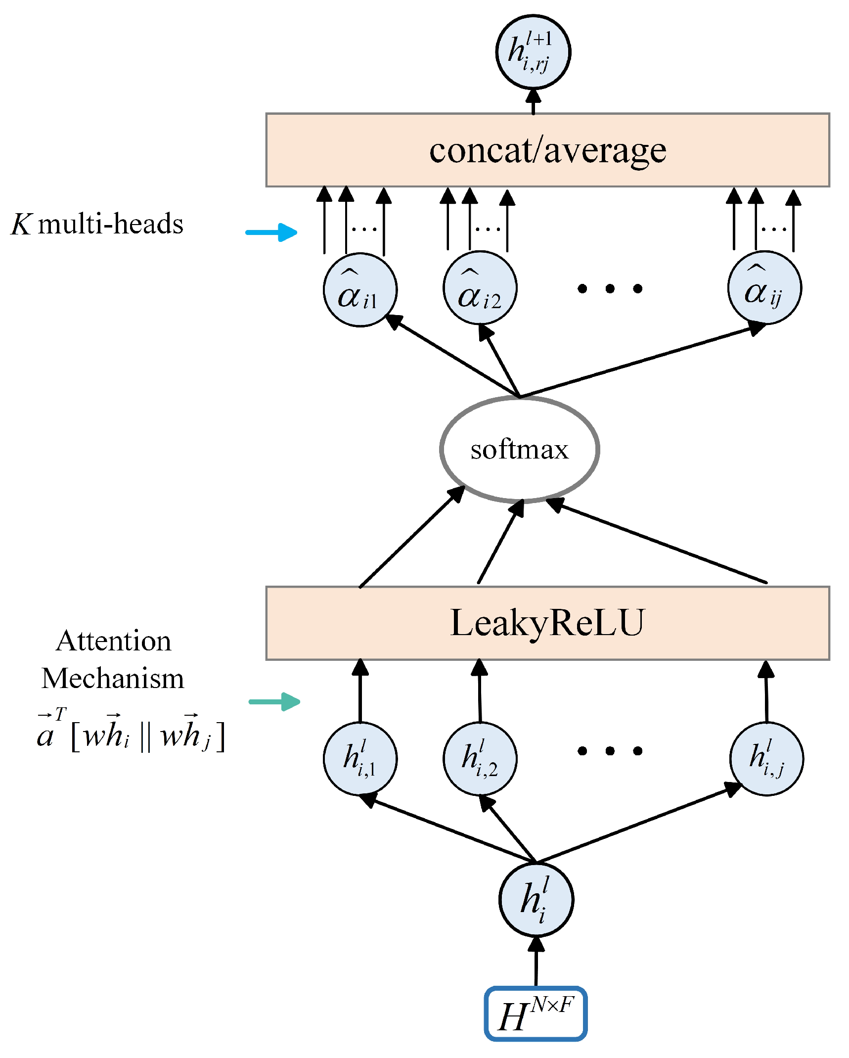
In real-world traffic networks, the spatial relationships between road nodes and their neighbouring nodes are dynamic, varying over time in response to fluctuating traffic conditions. GAT introduces an MSA mechanism to capture these evolving relationships by assigning different weights to node connections, enabling a more efficient representation of spatial features within the traffic network. Specifically, the attention mechanism dynamically adjusts the influence of neighbouring nodes by identifying the most relevant spatial dependencies at each step, enhancing the model’s ability to capture temporal variability in spatial relationships. Our model uses an MSA mechanism in the GAT framework, enabling it to learn attention coefficients from multiple subspaces simultaneously, which results in richer and more comprehensive spatial representations. The architecture of the GAT model is depicted in Figure 3.

At every time step, GAT first defines a feature transformation matrix $W\in R^{F\times F^{\prime }}$, which linearly transforms the input features of each node, thereby mapping them into a novel feature space, as shown:

$$h_i^l=W{h}_i$$

(5)

where $W$ is the trainable feature transformation matrix, $h_i$ and $h_i^l$ denote the input features of node $i$ and the new features after transformation at layer $l$, respectively.

Then, the attention mechanism calculates the weight between two connected nodes, denoted by:

$$e_{ij}=\mathrm{LeakyReLU}(a^T[h_i^l||h_j^l])$$

(6)

where $a$ is attention vector, $||$ indicates the concatenation of feature vectors, and $\mathrm{LeakyReLU}$ serves as the activation function to calculate the attention coefficient $e_{ij}$ by merging the features of node $i$ and node $j$, where $j$ is a neighbour of $i$, and since $i$ may have multiple neighbours, it is necessary to perform normalization, as defined by:

$${\alpha }_{ij}={\displaystyle \frac{\exp (e_{ij})}{{\displaystyle {\sum }_{k\in {\mathbb{N}}_i}\exp (e_{ik})}}}$$

(7)

where ${\mathbb{N}}_i$ is the set of neighbours of node $i$, and the attention weights ${\alpha }_{ij}$ are derived by applying $\mathrm{softmax}$ normalization to the attention coefficients.

The output of node $i$ are calculated by using the attention weights to aggregate the features of its neighbouring nodes, which can be computed by:

$$h_i^{l+1}=\sigma ({\displaystyle {\sum }_{j\in {\mathbb{N}}_i}{\alpha }_{ij}{h}_j^l})$$

(8)

where $\sigma$ is an activation function, $h_j^l$ denotes the features of neighbouring nodes, ${\alpha }_{ij}$ is the attention weight of node $j$ relative to node $i$. The new feature representation $h_i^{l+1}$ of node $i$ is obtained by aggregating the features from all neighbouring nodes.

The MSA mechanism strengthens the model’s capacity to capture a wide range of feature information, significantly improving its performance [25]. By allowing the model to focus on different aspects of the input features in multiple representation subspaces simultaneously, it produces the final output by combining the features from all attention heads, as shown:

$$h_i^{l+1}=|{|}_{k=1}^K\sigma ({\displaystyle {\sum }_{j\in {\mathbb{N}}_i}{\alpha }_{ij}^k{h}_j^l})$$

(9)

$$h_i^{l+1}=\sigma ({\displaystyle \frac{1}{K}}{\displaystyle {\sum }_{k=1}^K{\displaystyle {\sum }_{j\in {\mathbb{N}}_i}{\alpha }_{ij}^k{h}_j^l}})$$

(10)

where $l$ denotes the current layer, $K$ is the number of attention heads. For intermediate layers, Equation (9) is applied to concatenate the output features from each attention head. At the final output layer, Equation (10) is applied to average the concatenated features, producing the final output features.

3.3.2. Transfer Probability Matrix

The GAT model captures spatial relationships within the traffic network by evaluating the significance of neighbouring nodes to a central node at each time step, based on feature similarity. This enables the aggregation of spatial features from adjacent nodes. However, in real-world traffic networks, spatial interactions are influenced not only by feature similarity and connectivity but also by current traffic conditions. These conditions play a pivotal role in determining the effectiveness of feature transfer from neighbouring nodes to the target node and the target node’s capacity to receive these features. Therefore, our method incorporates the traffic state of nodes at the present step.

The traffic state of nodes is described using a congestion coefficient, which reflects the current congestion level. The congestion coefficient is calculated by:

$$c_i^t={\displaystyle \frac{v_{i,\max }-v_i^t}{v_{i,\max }}}\cdot {\displaystyle \frac{q_i^t}{q_{i,\max }}}\cdot {\displaystyle \frac{k_i^t}{k_{i,\max }}}$$

(11)

where $c_i^t$ is the congestion coefficient of node $i$ at time step $t$, $v_{i,\max }$ represents its maximum speed throughout the time series, $v_i^t$ is the average speed at that specific time, $q_{i,\max }$ refers to the maximum flow over the entire time series, $q_i^t$ is the flow at that moment, $k_{i,\max }$ is the maximum occupancy rate during the time series, and $k_i^t$ is the occupancy rate at that time.

Once the congestion coefficient is determined, the transfer coefficient is calculated to reflect the ability of a node to transmit and receive features. By introducing the transfer coefficient matrix, the model can more accurately reflect and capture the true spatial features of the road network. The calculation at the time step $t$ is calculated by:

$${\mathcal{l}}_i^t=1-c_i^t$$

(12)

where ${\mathcal{l}}_i^t$ is the transfer coefficient of node $i$, $c_i^t$ is the congestion coefficient of node $i$.

As shown in Figure 4, after obtaining the transfer coefficient for each node, the method calculates the transfer probability of adjacent nodes transmitting their features to the target node and then forms the transfer probability matrix. This calculation also accounts for the node’s self-connectivity, which represents the probability of the node maintaining its features unchanged, represented by congestion probability. The calculation of the transfer probability at each position in the transfer probability matrix is described as:

$$p_{ij}=\left\{\begin{array}{l}\begin{array}{cc}{\mathcal{l}}_i\cdot {\mathcal{l}}_j,& i\ne j\end{array}\\ \begin{array}{cc}{c}_i\cdot c_j,& i=j\end{array}\end{array}\right.$$

(13)

where $p_{ij}$ represents the transfer probability from nodes $j$ and $i$.

Conceptually, the transfer probability matrix extends beyond conventional attention-based weighting by incorporating traffic-state-dependent transmission capabilities. Unlike prior GAT-based approaches that rely solely on feature similarity, this mechanism reflects each node’s dynamic ability to transmit or retain features, thereby capturing asymmetric and time-varying spatial interactions within real traffic networks.

3.3.3. Distance Decay Matrix

While the transfer probability matrix quantifies each node’s dynamic transmission and retention ability, spatial interactions are also strongly influenced by geographical distance. As the spatial distance between nodes increases, their mutual influence weakens, resulting in a lower probability of successful feature transmission from neighbouring nodes to the target node.

Existing studies in traffic and mobility modelling similarly highlight the importance of distance-based attenuation. For instance, Wu et al. [26] employed anisotropic Gaussian process kernels to model spatial propagation in traffic state estimation, demonstrating that influence diminishes with distance and direction. Deng [27] proposed a spatio-temporal kernel approach that constructs adaptive spatio-temporal graphs based partly on distance-sensitive embeddings. Following these insights, we adopt the Gaussian kernel function as the distance decay function:

$$d_{ij}=\exp (-{\displaystyle \frac{{\mathrm{distance}}_{ij}^2}{2{\sigma }^2}})$$

(14)

where ${\mathrm{distance}}_{ij}$ represents the spatial distance from node $i$ to node $j$, while $\sigma$ denotes the standard deviation of the Gaussian kernel function, determined from the statistical data, and $d_{ij}$ signifies the distance decay factor between nodes $i$ and $j$. As the distance increases, the decay factor decreases, indicating a weakening influence between the nodes. This approach effectively quantifies how distance impacts the transmission of features, allowing for a more nuanced understanding of spatial features within the road network.

The adjacency matrix in the GAT model traditionally uses only binary values (0 and 1) to indicate whether two nodes are connected. This helps identify neighboring nodes but does not capture the intricacies of the spatial features in a road network. Such a simple representation limits the model’s capacity to fully express the complex nature of the network.

To address this limitation, this method replaces the adjacency matrix with a distance decay matrix, which incorporates a decay factor based on the distance between nodes. The decay factor allows the model to express varying degrees of connectivity, with closer nodes having stronger connections and distant nodes having weaker ones. This richer representation helps the model capture more detailed spatial features. The distance decay matrix is constructed as:

$$D=\left[\begin{array}{cccc}1& d_{12}& \dots & d_{1N}\\ d_{21}& 1& & d_{2N}\\ ⋮& & \ddots & ⋮\\ d_{N1}& d_{N2}& \dots & 1\end{array}\right]$$

(15)

To ensure self-connectivity, the diagonal elements of the distance decay matrix are set to 1, maintaining each node’s feature representation. This adjustment enables the model to better capture spatial features while also accounting for the complexity inherent in real-world traffic networks.

By jointly incorporating the transfer probability and distance decay matrices, the TA-GAT captures both the existence and strength of spatial connections, offering a more interpretable and realistic modelling of spatial influence.

3.3.4. Fusion

Finally, to integrate the transfer probability matrix and the distance decay matrix into the GAT module, both factors are embedded into the computation of neighbour node weights. By combining Equations (6), (13) and (14), the new weighting formulation is defined as:

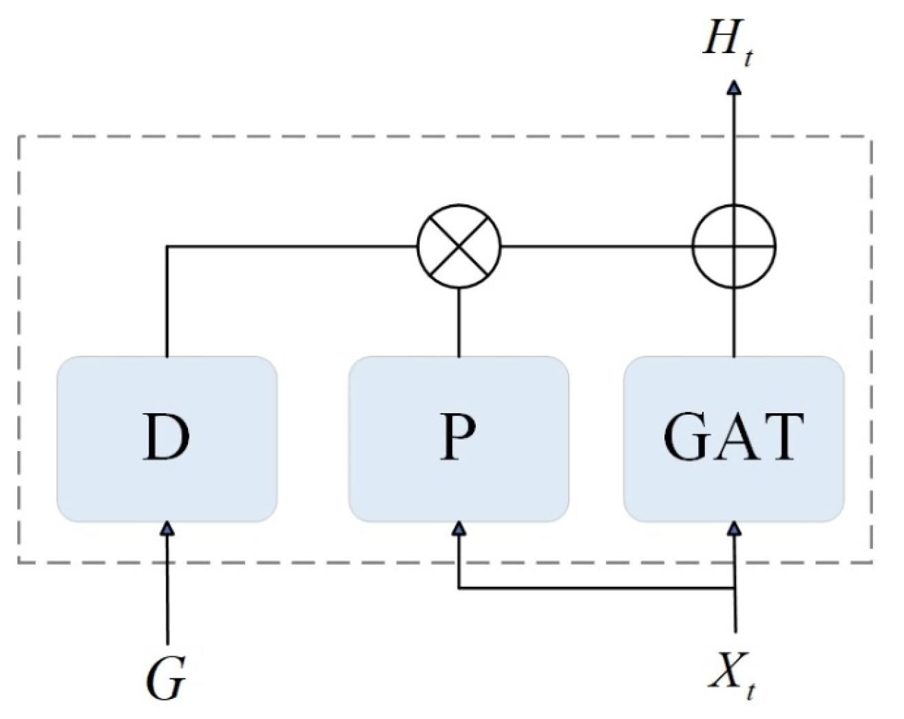
$${\widehat{e}}_{ij}=p_{ij}\cdot d_{ij}+\mathrm{LeakyReLU}(a^T[h_i^l||h_j^l])$$

(16)

where $p_{ij}$ is the transfer probability factor between nodes $i$ and $j$, $d_{ij}$ refers to the distance decay factor connecting nodes $i$ and $j$, and ${\widehat{e}}_{ij}$ is the improved weight coefficient for nodes $i$ and $j$.

Figure 5 illustrates the integrated TA-GAT module, where $D$ represents the distance decay matrix module, $P$ denotes the transfer probability matrix module, $\otimes$ represents the element-wise product of tensors, $\oplus$ refers to the element-wise addition of tensors. The module takes preprocessed traffic sequence data and the adjacency matrix as inputs, and outputs a new feature sequence after aggregating spatial information from neighbouring nodes. This fusion design enables the model to capture not only spatial proximity but also the dynamic transmission capability of each node, thereby improving its ability to represent real-world road network interactions more effectively.

3.4. Gating Network Module

The spatial features of road nodes are influenced by their neighboring nodes at the present time step and their features from the previous time step. To effectively integrate these aspects, a gating network is introduced after the TA-GAT. As illustrated in Figure 6, the feature sequence processed by the TA-GAT is fed into the gating network, which performs a weighted fusion of the spatial features from both time steps, yielding a new spatial feature representation for the current time step.

The calculation processes are shown as follows:

$$X_t=[H_{t-1},H_t]$$

(17)

$$G_t=\sigma (W_g\cdot X_t+b_g)$$

(18)

$${\widehat{H}}_t=G_t\odot H_t+(1-G_t)\odot H_{t-1}$$

(19)

where $[H_{t-1},H_t]$ are the spatial feature vectors at time step $t-1$ and $t$, $X_t$ denotes the concatenated vector of both time steps, $w_g$ represents the weight matrix, $b_g$ is the bias vector, $\sigma$ denotes the sigmoid function, and $G_t$ is the gating signal that adaptively adjusts the contributions from different time steps. Thus, ${\widehat{H}}_t$ is the new spatial feature vector after aggregating features from the preceding time step at time step $t$.

The inclusion of the gating network enhances the model’s expressive capability, enabling it to capture the dynamic variations more effectively in traffic flow and improve prediction accuracy. Additionally, this network performs an initial temporal aggregation of the feature sequence, facilitating the subsequent extraction of temporal features.

3.5. Temporal Feature Extraction Module

Traffic data exhibits significant temporal dependencies, and although RNNs are commonly used for learning these dependencies, they often face gradient explosion and vanishing gradient issues. LSTM addresses these issues by introducing gated units and cell states to regulate information flow [28]. However, as a sequential model, LSTM relies on previous time steps, leading to a gradual decay of hidden state information as the sequence length increases, which weakens its ability to capture global dependencies. In contrast, attention-based models like Transformer excel at this task.

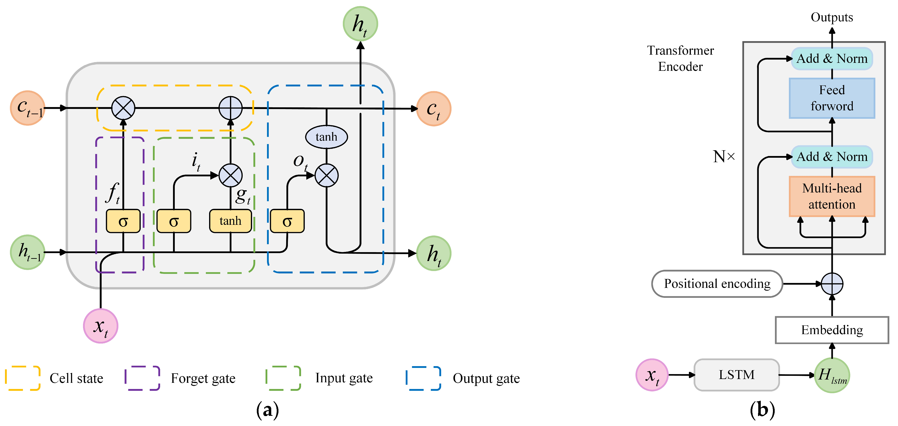
The MSA mechanism in Transformer enables direct interaction between different positions in the sequence, enabling a parallel model of global features through MSA. This study integrates a Transformer encoder with LSTM to extract both local and global temporal dependencies of traffic data. The structure is illustrated in Figure 7, with Figure 7a showing the LSTM structure and Figure 7b depicting the input and encoding layers of the Transformer. The encoding layer consists of multiple identical layers, each primarily composed of an MSA mechanism and a feedforward neural network (FFN).

First, the node spatial feature sequence processed by the TA-GAT and gating network is input into the LSTM. The calculation process of LSTM refers to the description by An and Dong [29]. Given the data $x_t$, the input feature representation is indicated as $H\in R^{T\times N\times F^{\prime }}$, where $F^{\prime }$ is the dimensionality of the feature output by TA-GAT. The cell state $c_t$ and hidden state $h_t$ can be calculated via:

$$i_t=\sigma (W_i\cdot [h_{t-1},x_t]+b_i)$$

(20)

$$f_t=\sigma (W_f\cdot [h_{t-1},x_t]+b_f)$$

(21)

$$g_t=\tanh (W_g\cdot [h_{t-1},x_t]+b_g)$$

(22)

$$o_t=\sigma (W_o\cdot [h_{t-1},x_t]+b_o)$$

(23)

$$c_t=f_t\cdot c_{t-1}+i_t\cdot g_t$$

(24)

$$h_t=o_t\cdot \tanh (c_t)$$

(25)

where $i_t$, $f_t$ and $o_t$ are the outputs of the input, forget, and output gates, respectively, $g_t$ is the candidate cell state, generating new information. $[h_{t-1},x_t]$ represents the concatenation of the previous hidden state and the current input, and the function $\tanh$ is the hyperbolic tangent activation. The matrices $W_i$, $W_f$, $W_g$, and $W_o$ represent the weight matrices, $b_i$, $b_f$, $b_g$, and $b_o$ denote the corresponding biases, $\sigma$ is the sigmoid activation function.

Next, the hidden state sequence $H_{lstm}$ output by the LSTM is used as input to the Transformer Encoder, which maps it into a learnable high-dimensional space through a linear transformation, represented as:

$$H_0=H_{lstm}{W}_e+b_e$$

(26)

where $W_e$ is the embedding matrix, $b_e$ is the bias term, and $H_0$ is the embedded representation. This sequence is then passed through a positional encoding layer, where positional information is encoded for each input in the sequence. The feature sequence ${H_0}^{\prime }$, now enriched with positional information, is fed into the encoder layer.

The core of the encoder layer is an MSA mechanism and a feedforward neural network. With the input ${H_0}^{\prime }$, the query $Q$, key $K$, and value $V$ subspaces are computed. The self-attention weights are then calculated by:

$$M=\mathrm{Softmax}({\displaystyle \frac{Q{K}^T}{\sqrt{D_k}}}V)$$

(27)

where Softmax is the normalization function, and $D_k$ is the input dimension divided by the number of attention heads, which prevents the Softmax function from saturating when gradients are minimal. $M$ represents the attention weights.

This process occurs independently for each attention head, utilizing the MSA mechanism to learn different dependency relationships from various potential subspaces.

The outputs from multiple single-head attentions are concatenated to create the MSA output, improving the model’s ability to express complex patterns. The FFN then processes this output by applying two linear transformations interspersed with an activation function, denoted by:

$$\mathrm{FFN}(x)=W_2\cdot \mathrm{RELU}(x{W}_1+b_1)+b_2$$

(28)

where $W_1$ and $W_2$ denote the weight matrices for the linear transformations, $b_1$ and $b_2$ refer to the bias vectors, and $\mathrm{RELU}$ is the activation function, with $x$ being the output of the MSA mechanism.

To accelerate training and prevent gradient instability, residual connections and layer normalization are applied after each self-attention and FFN layer. Finally, the Transformer Encoder’s output is passed to the FC layer that maps hidden states to the target output space, producing initial traffic flow predictions.

By combining the LSTM and Transformer, the model leverages both local temporal continuity and global contextual awareness, ensuring that short-term fluctuations and long-range patterns are jointly captured.

3.6. Training and Output Module

The predicted values generated by the FC layer are standardized. Denormalization is required to restore the non-stationary elements to the dataset and restore them to their original scale [30]. The denormalization process is expressed by:

$$y=y^{\prime }\cdot \sigma +\mu$$

(29)

where $y^{\prime }$ denotes the predicted values output by the FC layer, $\sigma$ represents the standard deviation obtained during normalization, $\mu$ indicates the mean derived from the normalization process, and $y$ is the final predicted value.

Subsequently, choosing mean squared error (MSE) as the loss function further optimizes the TAGAT-LSTM-trans, as expressed in:

$$loss={\displaystyle \frac{1}{N}}{\displaystyle \sum _{i\in N}|q_{t+p,i}-{\tilde{q}}_{t+p,i}{|}^2}$$

(30)

where $N$ denote the number of nodes, $q_{t+p,i}$ and ${\tilde{q}}_{t+p,i}$ are the actual and predicted traffic flow, respectively.

By minimizing the loss function, the model iteratively updates its parameters to enhance prediction accuracy. Once the loss function reaches a predefined threshold, the model selects the best-performing parameter set, and the corresponding predictions are output as the final traffic flow forecasts.

3.7. Method Summary

Most existing traffic flow forecasting methods tend to overlook node state information when modeling spatial dependencies and often suffer from information attenuation during temporal feature extraction. To address these limitations, this study proposes a transmission-aware spatio-temporal graph attention network.

The model introduces a transfer probability matrix and a distance decay matrix to represent spatial feature propagation between nodes as a probabilistic transmission process, providing a more interpretable and realistic characterization of spatial interactions. This approach advances the theoretical foundation of spatio-temporal graph learning by integrating state-dependent transmission capabilities.

Furthermore, a unified framework integrating TA-GAT, a gated network, and LSTM–Transformer is developed to systematically enhance the model’s capability to capture spatio-temporal dependencies and improve interpretability. This framework provides a novel approach for multi-scale spatio-temporal representation learning. The following section evaluates the model’s effectiveness and applicability on real-world public datasets.

4. Results

4.1. Datasets

The experiments are conducted on two real-world traffic datasets, originate from California’s Caltrans Performance Measurement System (PeMS). This comprehensive system monitors and gathers real-time traffic information from over 39,000 sensors on primary highways across the state.

PeMS collects data every 30 s, which is then summarized into 5 min intervals, leading to each sensor generating 288 data points every day. Additionally, road network structure data is derived from the connectivity status and actual distances between sensors.

To comprehensively evaluate the model’s performance, we perform experimental analysis on two datasets: PeMS03 and PeMS04.

Table 2. Dataset description.

Datasets	Sensors	Edges	Time
PeMS03	358	547	1 September 2018–30 November 2018
PeMS04	307	340	1 January 2018–28 February 2018

summarizes the basic information for the two datasets. The PeMS03 dataset comprises 358 sensors and 547 edges, recording data over 91 days from 1 September 2018, to 30 November 2018.

In contrast, the PeMS04 dataset consists of 307 sensors and 340 edges, recording data over 59 days spanning 1 January 2018, through 28 February 2018. The raw data includes three key indicators: traffic flow, speed, and occupancy, which are utilized for feature extraction in this study.

4.2. Experimental Settings

Consistent with other baseline models, the dataset was split into training, validation, and test sets with a ratio of 6:2:2. Both the historical and prediction windows were set to one hour. To ensure fair model comparisons and the reproducible results, all baseline models were configured and trained using the hyperparameter settings recommended in their original publications or official code repositories. On this basis, the hyperparameters of the proposed TAGAT-LSTM-trans model were tuned according to the validation set performance, and the final optimal configuration is presented in

Table 3. Model hyperparameters.

Module	Hyperparameters	Numbers
TAGAT	Hidden units	32
	Attention heads	2
LSTM	Hidden units	256
	Layers	2
Transformer	Hidden units	256
	Attention heads	4
Other	Batch size	50
	Learning rate	5 × 10−4
	Dropout	0.1

.

The TA-GAT module has 32 hidden units and 2 attention heads; the LSTM comprises 2 layers with 256 hidden units per layer; and the Transformer Encoder has 256 hidden units and 4 attention heads. The TAGAT-LSTM-trans model uses the Adam optimizer [31], setting the batch size to 50 and the learning rate to 5 × 10⁻⁴. In addition, to prevent overfitting, we employed early stopping and dropout mechanisms (dropout rate = 0.1) during the experiments.

4.3. Baselines

In order to evaluate the efficacy of the TAGAT-LSTM-trans, this study contrasts it with the following six baseline models:

(1)

ARIMA [32]: Autoregressive integrated moving average (ARIMA) model is a traditional temporal sequence analysis method widely used for short-term forecasting, particularly effective in handling linear trends and seasonal variations in data.

(2)

VAR [33]: Vector auto-regressive (VAR) model is a multivariate temporal sequence model used to analyze several interdependent temporal sequence data and the relationships among their components.

(3)

LSTM [34]: LSTM is a specialized type of RNN that effectively handles long-term dependency issues by introducing memory cells and forgetting mechanisms.

(4)

DCRNN [35]: Diffusion convolutional recurrent neural network (DCRNN) utilizes bidirectional random walks on a graph and recurrent neural networks to learn the spatio-temporal features of traffic flow.

(5)

ASTGCN(r) [36]: Attention-based spatial-temporal graph convolutional network (ASTGCN) integrate the spatio-temporal attention mechanism and convolution, capturing time-period dependencies across different time scales, including recent, daily, and weekly, through three components, with their outputs combined to generate the final predictions. For fairness, only the temporal block of the recent cycle is utilized to simulate periodicity.

(6)

STDSGNN [37]: Spatial–temporal dynamic semantic graph neural network (STDSGNN) constructs two types of semantic adjacency matrices using dynamic time warping and Pearson correlation, incorporates a dynamic aggregation method for feature weighting, and employs an injection-stacked structure to reduce over-smoothing and improve forecasting accuracy.

This study adopts two widely used performance metrics—Mean Absolute Error (MAE) and Root Mean Square Error (RMSE)—to evaluate model accuracy. MAE measures the average magnitude of prediction errors, while RMSE penalizes larger deviations more strongly, providing a more sensitive assessment of forecasting precision.

4.4. Experimental Results

Table 4. Comparison of the mean performance of various methods on PeMS03 and PeMS04.

Model	PeMS03		PeMS04
	MAE	RMSE	MAE	RMSE
ARIMA	23.07	40.62	37.84	59.03
VAR	23.65	38.26	33.76	51.73
LSTM	21.33 ± 0.24	35.11 ± 0.50	27.14 ± 0.20	41.59 ± 0.21
DCRNN	18.18 ± 0.15	30.31 ± 0.25	24.70 ± 0.22	38.12 ± 0.26
ASTGCN(r)	17.69 ± 1.43	29.66 ± 1.68	22.93 ± 1.29	35.22 ± 1.90
STDSGNN	16.20 ± 0.18	25.89 ± 0.62	20.82 ± 0.25	32.56 ± 0.55
TAGAT-LSTM-trans	14.99 ± 0.09	24.98 ± 0.12	19.49 ± 0.18	31.68 ± 0.22

Bold font indicates the best performance metrics among all results.

presents the mean performance of traffic flow forecasting for the TAGAT-LSTM-trans model and the baseline models mentioned above over the future hour in the PeMS03 and PeMS04. Bold font indicates the best performance metrics among all results. Overall, TAGAT-LSTM-trans demonstrates significantly superior prediction results compared to all baseline models across both datasets.

Classic statistical models such as ARIMA and VAR, though effective for linear relationships, struggle to capture the nonlinear and spatio-temporal dependencies inherent in traffic flow, resulting in the poorest prediction performance. Deep learning models such as LSTM yield better results by capturing sequential dependencies. Models like DCRNN, ASTGCN, and STDSGNN further improve performance by jointly modeling spatial and temporal correlations, underscoring the importance of integrated spatiotemporal learning. Among these, STDSGNN achieves the best baseline results, benefiting from its multi-head attention mechanism that strengthens spatio-temporal feature extraction.

Compared with STDSGNN, TAGAT-LSTM-trans reduces MAE by 1.74 and 1.38 and RMSE by 0.50 and 0.82 on PeMS03 and PeMS04, respectively. These improvements arise from the introduction of the transfer probability and distance decay matrices, which enable the adaptive adjustment of attention weights based on current node states and inter-node distances. Moreover, integrating the Transformer Encoder alleviates the long-term dependency decay problem typical of LSTM models, enhancing the model’s global temporal representation capability.

To further verify the statistical robustness, independent-sample t-tests were conducted against ASTGCN(r) and STDSGNN on both datasets. Results indicate that the performance gains of TAGAT-LSTM-trans are statistically significant (p < 0.01), confirming the model’s consistent advantage in both RMSE and MAE.

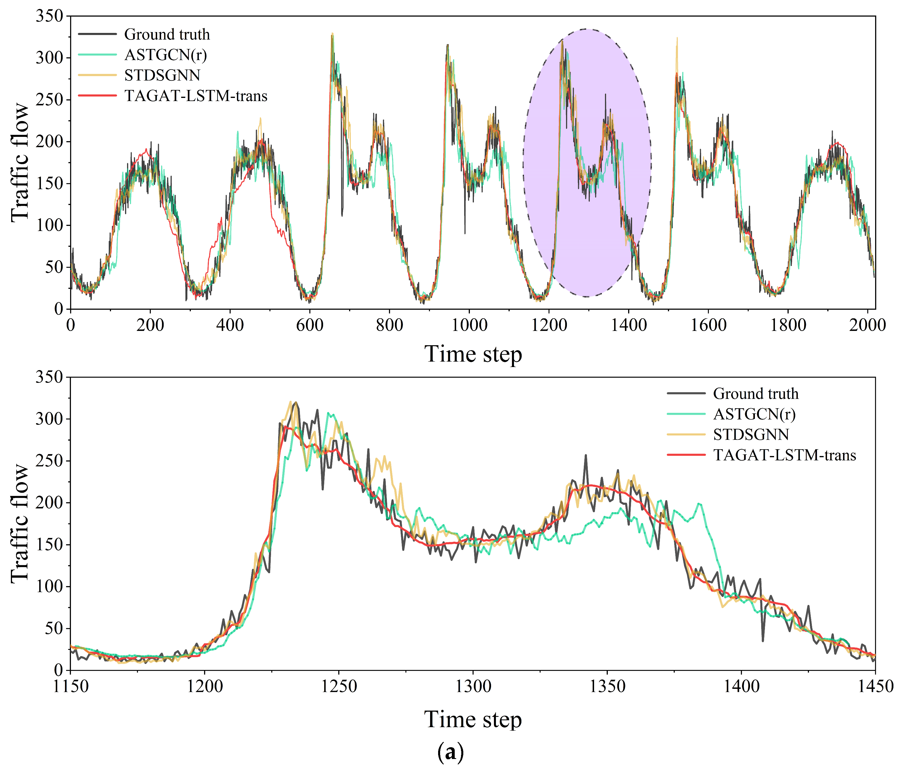
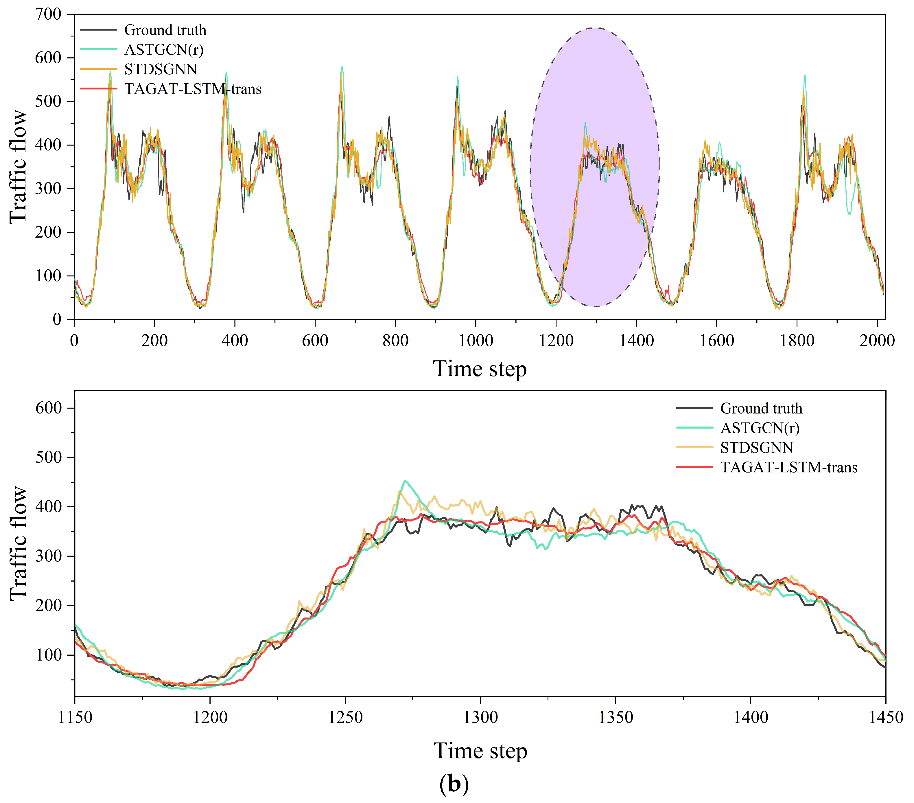
The prediction results of TAGAT-LSTM-trans on the PeMS03 and PeMS04 test sets are shown in Figure 8. To demonstrate the model’s performance, we randomly selected the prediction results of a specific node for visualization, providing an enlarged view of one day’s predictions. We compared TAGAT-LSTM-trans with two strong baseline models, ASTGCN(r) and STDSGNN, both of which are representative spatio-temporal deep learning models. In the figure, the black curve represents the ground truth, the green curve shows the predictions from ASTGCN(r), the yellow curve shows the predictions from STDSGNN, and the red curve corresponds to the predictions of our TAGAT-LSTM-trans. The purple-shaded area represents the zoomed-in region.

As can be observed from Figure 8, TAGAT-LSTM-trans effectively captures the dynamic variations in traffic flow. Particularly during periods of drastic fluctuation, the zoomed-in view clearly demonstrates that the prediction results of TAGAT-LSTM-trans are significantly closer to the ground truth than those of ASTGCN(r) and that they outperform STDSGNN in these volatile regions. This performance improvement primarily stems from the incorporation of the transfer probability matrix and the distance decay matrix during the spatial feature extraction stage. These components enable the model to better represent the transmission capacity and distance-sensitive dependencies between road nodes, thereby exhibiting stronger adaptability when confronted with abrupt changes in traffic states.

Figure 9 displays scatter plots of the TAGAT-LSTM-trans, ASTGCN(r), and STDSGNN across the two datasets, with the horizontal axis representing predicted values and the vertical axis representing actual values. Red dots indicate predictions from TAGAT-LSTM-trans, green dots represent ASTGCN(r) predictions, and yellow dots correspond to STDSGNN predictions. To clearly demonstrate the concentration and accuracy of each model’s forecasts, we added two error lines to the figure: the grey dashed line depicts the zero-error line, while the purple dashed lines indicate the 20% error margin. Points falling within the purple error lines have errors within 20% of the actual values, while points further away from the diagonal line indicate greater errors.

From the figure, it can be observed that the scatter plots of all three deep learning-based models exhibit a high degree of concentration along the diagonal, confirming their significant advantage over traditional methods. A detailed comparison reveals the superior performance of our proposed model: while STDSGNN and ASTGCN(r) already demonstrate strong accuracy, the scatter distribution of TAGAT-LSTM-trans is tighter and more aligned with the ideal fit line, particularly in the high-value regions (such as the range of 200–350 in the PeMS03 dataset and 400–600 in the PeMS04 dataset). This further confirms that TAGAT-LSTM-trans excels in capturing abrupt changes in traffic flow, demonstrating higher prediction accuracy.

4.5. Model Complexity and Computational Efficiency

To comprehensively evaluate the trade-off between model performance and computational cost, we compared the complexity of TAGAT-LSTM-trans against two representative baselines, ASTGCN(r) and STDSGNN.

Table 5. Model complexity and computational efficiency.

Model	Parameters	Size (MB)	Time/Iteration (ms)	Epochs to Convergence
ASTGCN(r)	45,0031	1.72	172.24 ± 9.5	200
STDSGNN	1,044,605	3.98	268.43 ± 1.2	200
TAGAT-LSTM-trans (Ours)	1,810,741	6.91	337.86 ± 19.44	~79

summarizes the number of trainable parameters, model size, and average training time per iteration.

However, a key finding is its significantly faster convergence speed. Leveraging an early-stopping mechanism, our model typically converges within approximately 79 epochs, less than half of the 200 epochs required by the baseline models for stable convergence. This rapid convergence substantially offsets the higher per-iteration cost, making the total computational investment manageable.

Combined with Table 4, these results indicate that the additional parameters are effectively utilized. The TAGAT-LSTM-trans model thus achieves a favorable balance between computational efficiency and predictive performance, delivering higher accuracy without incurring a prohibitive increase in overall training cost.

4.6. Ablation Studies

To strengthen the validation of the contribution of each module in the TAGAT-LSTM-trans model, we designed four variant models and tested them under optimal parameter settings, comparing their results with those of TAGAT-LSTM-trans on the PeMS03 and PeMS04 datasets. The distinctions between these four variant models are as follows:

(1)

Basic: This variant removes the transfer-aware (TA), gating network (GN), and Transformer Encoder (trans) modules, relying solely on GAT and LSTM to learn the spatio-temporal dependencies. It represents the most basic model configuration.

(2)

TA + GN: This variant omits the trans module to evaluate the necessity of capturing global temporal dependencies in traffic flow.

(3)

GN + trans: This variant excludes the TA module, assessing the importance of considering the transmission capacity of traffic features between nodes when aggregating spatial features from neighbouring nodes.

(4)

TA + trans: This variant eliminates the GN module to evaluate the impact of integrating spatial features of traffic flow from adjacent time steps.

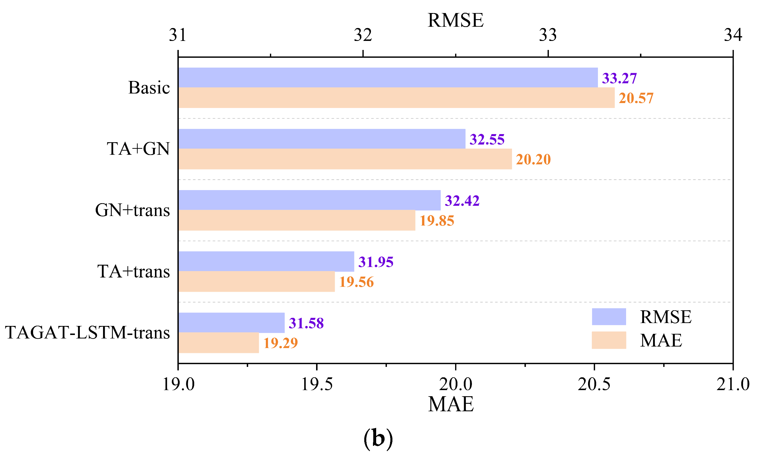
Figure 10 presents the results of the ablation experiments. Experimental results across both datasets clearly show that the predictions of TAGAT-LSTM-trans significantly outperform those of the four variant models, emphasizing the effectiveness of each module in enhancing the model’s performance.

Specifically, the Basic variant exhibits the worst prediction accuracy. By removing the TA, GN, and trans modules, this variant relies solely on GAT and LSTM to learn the spatio-temporal dependences of traffic flow, its simplified structure is unable to effectively learn the complex variations in traffic flow, resulting in poor predictions. The TA + GN variant, which omits the trans module and depends exclusively on LSTM for capturing temporal dependencies, shows the second-worst performance. Compared to TAGAT-LSTM-trans, these variants experience an increase in MAE by 0.48 and 0.91, and in RMSE by 0.72 and 0.97 across the two datasets. This highlights the crucial role of the trans module in temporal feature extraction, which has the most significant impact among the three modules.

For the GN + trans variant, although the trans module is reintroduced, the absence of the TA module fails to consider each node’s ability to propagate its traffic characteristics, leading to suboptimal spatial feature extraction. As a result, the MAE for these variant increases by 0.4 and 0.56, while RMSE increases by 0.44 and 0.84 on the two datasets compared to TAGAT-LSTM-trans, underscoring the necessity of modelling the transmission probabilities of traffic features between nodes.

Lastly, the TA + trans variant, which retains the TA module for considering node transmission probabilities and the trans module for capturing global temporal dependencies, achieves the best performance among the four variants. However, its MAE increases by 0.32 and 0.27, and RMSE by 0.39 and 0.37 on the two datasets compared to TAGAT-LSTM-trans. This performance decline is due to removing the GN module, which is responsible for further integrating spatial features from adjacent time steps and capturing the temporal dynamics of spatial features, ultimately enhancing the model’s predictive capability.

5. Discussion

This section provides a comprehensive interpretation of the experimental results, discussing the theoretical implications, practical significance, and limitations of the proposed TAGAT-LSTM-trans model.

5.1. Performance Superiority and Mechanism Interpretation

The TAGAT-LSTM-trans model demonstrates consistently superior performance over all baselines, achieving the lowest RMSE and MAE across both the PeMS03 and PeMS04 datasets. These improvements are not only statistically significant (p < 0.01) but also practically meaningful. Recent studies have highlighted the effectiveness of hybrid spatio-temporal models, such as the CCNN-former [38], which integrates CNNs and Transformers for image-based traffic prediction, and the Cross-IDR framework [39], which addresses cross-city transfer learning through incremental distribution rectification. However, unlike conventional attention-based graph models that rely solely on feature correlations, our model establishes a differentiated advantage by integrating a transfer probability matrix and a distance decay matrix into the graph attention framework. This design enhances the physical interpretability and adaptive modeling capacity of the network: the transfer matrix enables dynamic adjustment of node influence according to current congestion levels, whereas the distance decay matrix quantitatively represents spatial attenuation effects. Together, these mechanisms allow for a more realistic representation of how traffic features propagate throughout the network.

Compared to conventional GATs, which lack explicit reasoning based on traffic states, and GCNs, which often struggle with heterogeneous spatial features and over-smoothing, our approach embeds physical constraints directly into the attention mechanism. This proves particularly important for capturing abrupt changes in traffic flow (as visualized in Figure 8), scenarios in which models such as ASTGCN(r) and STDSGNN show limitations. Furthermore, while intercity mobility research often emphasizes distinct patterns such as low-frequency travel and holiday deviations [40], our model’s focus on dynamic, node-level transmission capacity provides finer-grained adaptability under both recurrent and irregular traffic conditions. The model’s strong adaptability under fluctuating conditions further demonstrates that TAGAT-LSTM-trans not only fits stable patterns but also effectively captures abrupt flow changes. This finding suggests that integrating interpretable physical constraints into deep learning models can substantially improve robustness and responsiveness in real-world traffic systems.

5.2. Component Contributions and Functional Synergy

The ablation experiments indicate that each component contributes distinct yet complementary strengths to the overall architecture. The TA-GAT module, which incorporates the transfer probability and distance decay matrices, addresses a key limitation of static GCNs and adaptive GATs, namely their limited ability to model spatial propagation that varies with traffic states. The LSTM preserves short-term temporal continuity, a strength of RNN-based models observed in traffic volume prediction studies [41], but this capability is often insufficient in temporal models that rely solely on self-attention. The gating network further ensures temporal continuity between adjacent time steps, facilitating smoother transitions in spatial features and strengthening temporal coherence.

The inclusion of the Transformer Encoder helps mitigate the long-term dependency decay problem common in RNN-based models, a finding consistent with the CCNN-former model, where parallelizable self-attention improves the extraction of global temporal context. Consequently, our hybrid design aligns with the emerging trend of coupling recurrent local modeling with attention-based global temporal reasoning, as seen in models like PDFormer [42], and extends it through spatially interpretable graph attentional mechanisms.

5.3. Limitations

Although the TAGAT-LSTM-trans model demonstrates strong performance in traffic flow forecasting, we acknowledge several limitations and potential biases related to its methodology, data, and design.

First, data representativeness and geographical structural bias remain important considerations. The evaluation in this study primarily relies on the PeMS freeway datasets, which feature regularly structured networks and stable sensor deployment. This may introduce geographical bias, as the model’s generalization capability to more complex urban road networks or cities with sparse sensor coverage remains unverified. Additionally, sensor noise and missing values in PeMS data may be amplified by the transfer-aware attention mechanism, potentially introducing data-driven prediction biases.

Second, there exists a trade-off between interpretability and flexibility in the model design. While the transfer probability matrix and distance decay matrix enhance the interpretability in the spatial feature propagation, this parameterization may not fully capture more nuanced spatial interactions within multi-level or complex non-Euclidean urban structures. Moreover, the model does not explicitly incorporate external factors, such as weather variation, traffic incidents or large-scale events, which may reduce robustness under anomalous traffic conditions.

Finally, a trade-off between computational efficiency and performance is also present. While the multi-component architecture integrating TA-GAT, the gating mechanism and the LSTM–Transformer encoder improves prediction accuracy, it increases model complexity and computational cost, potentially limiting applicability in large-scale road networks or real-time scenarios [43]. In addition, although attention mechanisms enhance feature extraction capabilities, their internal decision-making processes remain partially opaque, potentially introducing model-driven uncertainty during deployments, a challenge that is common in many deep learning models.

While the model improves predictive accuracy, translating its forecasts into actionable traffic management strategies, such as signal timing control and route optimization, remains an important direction for future research. Developing a closed-loop system that links high-accuracy prediction with real-time decision-making represents a significant yet unresolved challenge in intelligent transportation, highlighting the persistent gap between prediction and decision-oriented applications.

6. Conclusions

This paper presents the TAGAT-LSTM-trans model, a transfer-aware spatio-temporal graph attention network specifically designed for traffic flow forecasting. The model effectively integrates transmission probability modelling, gated temporal fusion, and hybrid LSTM–Transformer encoding to capture both dynamic spatial dependencies and global temporal correlations. Experimental results demonstrate that this model significantly outperforms existing baseline across multiple datasets.

This work contributes to advancing intelligent transportation management by providing a more interpretable and adaptive modelling framework for dynamic road networks. Future research will focus on incorporating external factors including weather conditions, traffic incidents, and emergencies to refine the modelling of the transfer probability matrix. In addition, the framework will be extended to broader spatio-temporal forecasting scenarios, such as lane-level prediction, to support fine-grained traffic planning and congestion management.

References

1. Cao, S.; Wu, L.; Wu, J.; Wu, D.; Li, Q. A spatio-temporal sequence-to-sequence network for traffic flow prediction. Inf. Sci. 2022, 610, 185–203. [Google Scholar] [CrossRef]
2. Zhang, J.; Zheng, Y.; Qi, D.; Li, R.; Yi, X.; Li, T. Predicting citywide crowd flows using deep spatio-temporal residual networks. Artif. Intell. 2018, 259, 147–166. [Google Scholar] [CrossRef]
3. Lv, M.; Hong, Z.; Chen, L.; Chen, T.; Zhu, T.; Ji, S. Temporal multi-graph convolutional network for traffic flow prediction. IEEE Trans. Intell. Transp. Syst. 2020, 22, 3337–3348. [Google Scholar] [CrossRef]
4. Boukerche, A.; Wang, J. Machine learning-based traffic prediction models for intelligent transportation systems. Comput. Netw. 2020, 181, 107530. [Google Scholar] [CrossRef]
5. Zhuang, W.; Cao, Y. Short-term traffic flow prediction based on cnn-bilstm with multicomponent information. Appl. Sci. 2022, 12, 8714. [Google Scholar] [CrossRef]
6. Lecun, Y.; Bengio, Y.; Hinton, G. Deep learning. Nature 2015, 521, 436–444. [Google Scholar] [CrossRef] [PubMed]
7. Ren, C.; Chai, C.; Yin, C.; Ji, H.; Cheng, X.; Gao, G.; Zhang, H. Short-Term Traffic Flow Prediction: A Method of Combined Deep Learnings. J. Adv. Transp. 2021, 2021, 9928073. [Google Scholar] [CrossRef]
8. Zhang, W.; Yu, Y.; Qi, Y.; Shu, F.; Wang, Y. Short-Term Traffic Flow Prediction Based on Spatio-Temporal Analysis and CNN Deep Learning. Transp. A Transp. Sci. 2019, 15, 1688–1711. [Google Scholar] [CrossRef]
9. Jian-xi, Y.; Chao-shun, Y.U.; Ren, L.I. Traffic network speed prediction via multi-periodic-component spatial-temporal neural network. J. Transp. Syst. Eng. Inf. Technol. 2021, 21, 112. [Google Scholar]
10. Narmadha, S.; Vijayakumar, V. Spatio-Temporal vehicle traffic flow prediction using multivariate CNN and LSTM model. Mater. Today Proc. 2023, 81, 826–833. [Google Scholar] [CrossRef]
11. Peng, H.; Du, B.; Liu, M.; Liu, M.; Ji, S.; Wang, S.; Zhang, X.; He, L. Dynamic graph convolutional network for long-term traffic flow prediction with reinforcement learning. Inf. Sci. 2021, 578, 401–416. [Google Scholar] [CrossRef]
12. Luan, S.; Ke, R.; Huang, Z.; Ma, X. Traffic congestion propagation inference using dynamic Bayesian graph convolution network. Transp. Res. Part C Emerg. Technol. 2022, 135, 103526. [Google Scholar] [CrossRef]
13. Qu, Z.; Liu, X.; Zheng, M. Temporal-spatial quantum graph convolutional neural network based on Schrödinger approach for traffic congestion prediction. IEEE Trans. Intell. Transp. Syst. 2022, 24, 8677–8686. [Google Scholar] [CrossRef]
14. Wang, Y.; Jing, C.; Xu, S.; Guo, T. Attention based spatiotemporal graph attention networks for traffic flow forecasting. Inf. Sci. 2022, 607, 869–883. [Google Scholar] [CrossRef]
15. Fu, R.; Zhang, Z.; Li, L. Using LSTM and GRU neural network methods for traffic flow prediction. In Proceedings of the 2016 31st Youth Academic Annual Conference of Chinese Association of Automation (YAC), Wuhan, China, 11–13 November 2016; pp. 324–328. [Google Scholar]
16. Zheng, C.; Fan, X.; Wen, C.; Chen, L.; Wang, C.; Li, J. DeepSTD: Mining spatio-temporal disturbances of multiple context factors for citywide traffic flow prediction. IEEE Trans. Intell. Transp. Syst. 2019, 21, 3744–3755. [Google Scholar] [CrossRef]
17. Veličković, P.; Cucurull, G.; Casanova, A.; Romero, A.; Lio, P.; Bengio, Y. Graph attention networks. arXiv 2017, arXiv:1710.10903. [Google Scholar]
18. Gan, R.; An, B.; Li, L.; Qu, X.; Ran, B. A freeway traffic flow prediction model based on a generalized dynamic spatio-temporal graph convolutional network. IEEE Trans. Intell. Transp. Syst. 2024, 25, 13682–13693. [Google Scholar] [CrossRef]
19. Ali, A.; Ullah, I.; Ahmad, S.; Wu, Z.; Li, J.; Bai, X. An attention-driven spatio-temporal deep hybrid neural networks for traffic flow prediction in transportation systems. IEEE Trans. Intell. Transp. Syst. 2025, 26, 14154–14168. [Google Scholar] [CrossRef]
20. Chen, Y.; Huang, J.; Xu, H.; Guo, J.; Su, L. Road traffic flow prediction based on dynamic spatiotemporal graph attention network. Sci. Rep. 2023, 13, 14729. [Google Scholar] [CrossRef]
21. Lu, K.F.; Liu, Y.; Peng, Z.-R. Assessing the impacts of transit systems and urban street features on bike-sharing ridership: A graph-based spatiotemporal analysis and prediction model. J. Transp. Geogr. 2025, 128, 104356. [Google Scholar] [CrossRef]
22. Wang, Q.; Ma, Z.; Yang, X.; Chien, S.I.-J.; Zhang, S.; Yin, Y. Exploring spatiotemporal dynamic of metro ridership and the influence of built environment factors at the station level: A case study of Nanjing, China. J. Transp. Geogr. 2025, 129, 104440. [Google Scholar] [CrossRef]
23. Cui, M.; Yu, L.; Nie, S.; Dai, Z.; Ge, Y.-E.; Levinson, D. How do access and spatial dependency shape metro passenger flows. J. Transp. Geogr. 2025, 123, 104069. [Google Scholar] [CrossRef]
24. Chen, X.; Wu, S.; Shi, C.; Huang, Y.; Yang, Y.; Ke, R.; Zhao, J. Sensing data supported traffic flow prediction via denoising schemes and ANN: A comparison. IEEE Sens. J. 2020, 20, 14317–14328. [Google Scholar] [CrossRef]
25. Vaswani, A.; Shazeer, N.; Parmar, N.; Uszkoreit, J.; Jones, L.; Gomez, A.; Kaiser, L.; Polosukhin, I. Attention is all you need. Adv. Neural Inf. Process. Syst. 2017, 30. [Google Scholar] [CrossRef]
26. Wu, F.; Cheng, Z.; Chen, H.; Qiu, Z.; Sun, L. Traffic state estimation from vehicle trajectories with anisotropic Gaussian processes. Transp. Res. Part C Emerg. Technol. 2024, 163, 104646. [Google Scholar] [CrossRef]
27. Deng, H. Traffic-Forecasting Model with Spatio-Temporal Kernel. Electronics 2025, 14, 1410. [Google Scholar] [CrossRef]
28. Gers, F.A.; Schmidhuber, J.; Cummins, F. Learning to forget: Continual prediction with LSTM. Neural Comput. 2000, 12, 2451–2471. [Google Scholar] [CrossRef]
29. An, Q.; Dong, M. Design and Case Study of Long Short Term Modeling for Next POI Recommendation. Int. J. Eng. Res. Manag. 2024, 11, 18–21. [Google Scholar]
30. Li, S.; Cui, Y.; Xu, J.; Li, L.; Meng, L.; Yang, W.; Zhang, F.; Zhou, X. Unifying Lane-Level Traffic Prediction from a Graph Structural Perspective: Benchmark and Baseline. arXiv 2024, arXiv:2403.14941. [Google Scholar] [CrossRef]
31. Kingma, D.P. Adam: A method for stochastic optimization. arXiv 2014, arXiv:1412.6980. [Google Scholar]
32. Williams, B.M.; Hoel, L.A. Modeling and forecasting vehicular traffic flow as a seasonal ARIMA process: Theoretical basis and empirical results. J. Transp. Eng. 2003, 129, 664–672. [Google Scholar] [CrossRef]
33. Zivot, E.; Wang, J. Vector Autoregressive Models for Multivariate Time Series. In Modeling Financial Time Series with S-PLUS®; Springer: Berlin/Heidelberg, Germany, 2006; pp. 385–429. [Google Scholar]
34. Hochreiter, S. Long Short-term Memory. Neural Comput. 1997, 9, 1735–1780. [Google Scholar] [CrossRef] [PubMed]
35. Li, Y.; Yu, R.; Shahabi, C.; Liu, Y. Diffusion convolutional recurrent neural network: Data-driven traffic forecasting. arXiv 2017, arXiv:1707.01926. [Google Scholar]
36. Guo, S.; Lin, Y.; Feng, N.; Song, C.; Wan, H. Attention based spatial-temporal graph convolutional networks for traffic flow forecasting. In Proceedings of the AAAI Conference on Artificial Intelligence, Honolulu, HI, USA, 27 January–1 February 2019; pp. 922–929. [Google Scholar]
37. Zhang, R.; Xie, F.; Sun, R.; Huang, L.; Liu, X.; Shi, J. Spatial-temporal dynamic semantic graph neural network. Neural Comput. Appl. 2022, 34, 16655–16668. [Google Scholar] [CrossRef]
38. Liu, L.; Wu, M.; Lv, Q.; Liu, H.; Wang, Y. CCNN-former: Combining convolutional neural network and Transformer for image-based traffic time series prediction. Expert Syst. Appl. 2025, 268, 126146. [Google Scholar] [CrossRef]
39. Yang, B.; Li, R.; Wang, Y.; Xiang, S.; Zhu, S.; Dai, C.; Dai, S.; Guo, B. Cross-city transfer learning for traffic forecasting via incremental distribution rectification. Knowl. Based Syst. 2025, 315, 113336. [Google Scholar] [CrossRef]
40. Yu, W.; Wang, W.; Hua, X.; Zhao, D.; Ngoduy, D. Dynamic patterns of intercity mobility and influencing factors: Insights from similarities in spatial time-series. J. Transp. Geogr. 2025, 124, 104154. [Google Scholar] [CrossRef]
41. Pranolo, A.; Saifullah, S.; Utama, A.B.; Wibawa, A.P.; Bastian, M. High-performance traffic volume prediction: An evaluation of RNN, GRU, and CNN for accuracy and computational trade-offs. BIO Web Conf. 2024, 148, 02034. [Google Scholar] [CrossRef]
42. Jiang, J.; Han, C.; Zhao, W.X.; Wang, J. Pdformer: Propagation delay-aware dynamic long-range transformer for traffic flow prediction. In Proceedings of the AAAI Conference on Artificial Intelligence, Washington, DC, USA, 7–14 February 2023; Volume 37, pp. 4365–4373. [Google Scholar]
43. Sun, F.; Hao, W.; Zou, A.; Cheng, K. TVGCN: Time-varying graph convolutional networks for multivariate and multifeature spatiotemporal series prediction. Sci. Prog. 2024, 107, 00368504241283315. [Google Scholar] [CrossRef]
Figure 1. Spatial feature correlation of traffic flow at road nodes.
Ijgi 14 00459 g001
Figure 2. The framework of the TAGAT-LSTM-trans model.
Ijgi 14 00459 g002
Figure 3. GAT model with a multi-head attention mechanism.
Ijgi 14 00459 g003
Figure 4. Node transfer probability diagram.
Ijgi 14 00459 g004
Figure 5. The TA-GAT module.
Ijgi 14 00459 g005
Figure 6. Gating Network diagram.
Ijgi 14 00459 g006
Figure 7. The LSTM-Trans module. (a) LSTM (b) Transformer Encoder.
Ijgi 14 00459 g007
Figure 8. Comparison of prediction results on PeMS03 and PeMS04. (a) Results on PeMS03; (b) Results on PeMS04.
Ijgi 14 00459 g008aIjgi 14 00459 g008b
Figure 9. Comparison of scatter plot on PeMS03 and PeMS04. (a) Scatter plot on PeMS03; (b) Scatter plot on PeMS04.
Ijgi 14 00459 g009
Figure 10. Results of ablation experiments on PeMS03 and PeMS04. (a) PeMS03; (b) PeMS04.
Ijgi 14 00459 g010aIjgi 14 00459 g010b