Article

A Spatial Planning Model for Obnoxious Facilities with Spatially Informed Constraints

Department of Geography and Sustainability, University of Tennessee, Knoxville, TN 37996, USA
*
Author to whom correspondence should be addressed.
ISPRS Int. J. Geo-Inf. 2025, 14(11), 449; https://doi.org/10.3390/ijgi14110449 (registering DOI)
Submission received: 21 August 2025 / Revised: 3 November 2025 / Accepted: 13 November 2025 / Published: 15 November 2025

Abstract

This research aims to develop a novel spatial optimization model for locating obnoxious facilities. While various obnoxious facility location problems (OFLP) have been introduced, the optimal spatial arrangements in existing models may not adequately reflect the real-world conditions, such as the distribution of population and locational restrictions across areas in a region, often offering extreme peripheral or clustered recommendations that ignore such conditions. To address this gap, this research introduces an alternative location model named the Spatially Informed Obnoxious Location (SI-OBNOX) model. The SI-OBNOX model was developed to address the extreme spatial arrangements produced by existing models by incorporating a unique set of constraints derived from the spatial characteristics of a planning region. The constraints integrate spatial–statistical measures into the model formulation to restrict extreme facility location behaviors, resulting in more reasonably distributed obnoxious facility sites while avoiding residential areas for them. The findings demonstrate that the spatial arrangements generated by the SI-OBNOX model outperform those of existing OFLPs in terms of three planning-related indices, namely separation, externality, and proximity, based on a case study of the East Tennessee region. The SI-OBNOX model can be adapted to other planning contexts where it is necessary to locate undesirable yet essential facilities for public welfare.

1. Introduction

The obnoxious facility location problem (hereafter OFLP) focuses on identifying suitable locations for undesirable facilities that negatively impact their surrounding neighborhoods. Facilities such as waste management plants [1,2,3], power stations [4,5], and transportation infrastructures [6,7,8] exemplify such obnoxious facilities due to their potential adverse effects on citizens’ quality of life and their communities. Given their hazardous, noxious, or otherwise undesirable nature, these facilities must be placed relatively far from populated areas, and they are referred to as obnoxious facilities [9].
While many public and private facilities aim to benefit their surrounding communities, obnoxious facilities exhibit a combination of positive and negative effects. For instance, waste management systems provide essential services for handling regional solid waste but also impose negative externalities such as noise, an unpleasant smell, and soil pollution. Planners must carefully balance these opposing effects when determining locations for such facilities. However, OFLPs remain relatively underexplored in the spatial optimization literature due to their ambivalent nature. The issue of locating obnoxious facilities is gaining prominence due to its relevance in real-world concerns, such as NIMBY (Not In My Back Yard) conflicts, where maintaining an adequate distance from communities is critical [9,10].
A critical limitation in applying existing OFLPs to practical planning contexts is their model behavior, which often results in impractical siting and allocation decisions. Such outcomes typically place obnoxious facilities either very close to densely populated residential areas or at the extreme outskirts of the planning region. Most OFLPs are formulated as mixed-integer programming (MIP) models that maximize either the separation distance between obnoxious facilities or the travel distance from obnoxious facilities to demand nodes. While the results are mathematically optimal, such strict canonical formulations often produce extreme spatial arrangements of selected facilities, exemplified by excessive peripheral placement or tightly clustered facility locations. These spatial patterns are undesirable for public service facility planning because they generate negative externalities for surrounding neighborhoods and degrade the efficiency of service provision. This challenge affects not only the siting of undesirable facilities such as waste management sites but also the broader evaluation of overall system performance, which is discussed in Section 2.
To overcome the limited capabilities of existing OFLP models, spatial statistical measures can be incorporated into facility location planning. Spatial statistics provide valuable insights into spatial heterogeneity by examining the distribution of attributes (e.g., population) and their inherent spatial autocorrelation, which reflects the characteristics of spatial association among geographic units within a planning space. In particular, local spatial statistics such as Getis–Ord’s Gi* or local Moran’s I effectively capture spatial autocorrelation at the individual-unit level. Integrating these measures into spatial optimization frameworks enables an effective representation of spatial heterogeneity and thereby improves the quality of the optimal solutions for the planning context.
However, employing spatial statistical measurements in spatial optimization problems has not been addressed much in previous studies. A number of recent studies, utilizing the spatially informed approach, have attempted to address the ability and usefulness of spatial statistical measures to solve spatial optimization problems in terms of computational performance [11,12,13,14]. They demonstrated that spatial information derived from spatial statistical measures can be integrated into MIP models to enhance computational efficiency in solving spatial optimization problems. To the best of our knowledge, no previous studies have integrated spatial statistical methodologies with spatial optimization models to improve location–allocation behavior and achieve more reasonable facility location planning, thereby enhancing the applicability of OFLP models.
In this context, this study introduces an alternative spatial optimization model for locating obnoxious facilities, named the Spatially Informed Obnoxious Location (SI-OBNOX) model. As we discuss in the next section, many OFLP variants face critical issues regarding the practicality of their solutions for spatial decision-making, as the optimal solutions often exhibit extreme spatial arrangements of facilities—either the excessive dispersal or clustering of obnoxious facilities—while ignoring the spatial associations in population distribution. The SI-OBNOX model addresses these inherent behavioral limitations of existing OFLP models by generating more regularly distributed facility locations that avoid densely populated areas while at the same time ensuring planning efficiency, as exemplified in the case of waste management systems. The SI-OBNOX model leverages spatial statistical methods to incorporate additional spatial information into the model formulation, as a form of constraints in which the characteristics of spatial autocorrelation are prescribed to reflect the realistic location behavior of obnoxious facilities. These constraints enhance the model’s ability to generate pragmatic but optimal solutions for locating obnoxious facilities given that virtually none of the existing studies address the analysis of location–allocation behaviors of OFLPs and seek more applicable solutions. In short, the SI-OBNOX model proposed in this study bridges the gap between theoretical modeling and practical facility location planning by evaluating its performance relative to traditional OFLPs. Comparison with other classes of OFLPs is provided to evaluate the effectiveness of the proposed model in terms of planning perspective with the following research questions:
  • RQ 1: How can spatial information influence the behavior of OFLPs, and how can it be incorporated into the model specification?
  • RQ 2: How does a SI-OBNOX model exhibit different behavioral characteristics compared to the existing OFLPs?
  • RQ 3: To what extent does a SI-OBNOX model improve various planning-related indices over the existing OFLPs?
By addressing these research questions, this study makes multiple contributions. First, it demonstrates the applicability of the SI-OBNOX model as an alternative to traditional OFLPs, offering a more practical and balanced approach to spatial decision-making for obnoxious facility siting. Second, it critically examines the intrinsic behavioral issues of various OFLP models—problems that have largely been overlooked in the literature—thus providing a foundation for improving solution approaches not only in OFLPs but also in broader classes of location-allocation problems.

2. Background and Literature

2.1. Existing OFLP Models

Several previous studies have addressed OFLPs using spatial optimization approaches. The article [9] provided a thorough systematic review of OFLPs, including both discrete and continuous models. They claimed that two distinct types of problems are considered part of the OFLPs, based on the following negative impacts: (1) negative interactions between the facilities themselves and (2) negative effects on neighboring communities. As this research does not aim to provide a comprehensive review of the existing literature on obnoxious facility location, we do not include the formulations of each spatial optimization model. In this section, we examine critical spatial optimization models for obnoxious facility location, especially in discrete space, because scrutinizing existing OFLP models is essential for developing an alternative model for locating obnoxious facilities and comparing it to traditional approaches. Those seeking mathematical formulations can refer to the original literature on the respective models. We first address the main characteristics of OFLPs and continue to examine the general location behavior of existing OFLP models and their main drawbacks, which is the main reason that we establish the SI-OBNOX model.
The first type of OFLP, commonly categorized as dispersion-based spatial optimization problems, includes the p-dispersion problem [15,16], maxisum dispersion [16], the p-defense problem [17,18], and the anti-covering location problem [19]. While these problems were formulated with different modeling goals, they share a common focus on facility dispersion. This class of problems is particularly useful for locating obnoxious facilities, where minimizing negative interactions among facilities is a critical concern, or facilities requiring mandatory separation standards. The authors of [20] formalized the classification of dispersion-based location models using two key criteria [21], consisting of (1) the specific goal of the objective function and (2) the consideration of separation or interaction among selected facilities (see [20] for details). For example, the p-dispersion problem [15,16] is one of the pioneering models in dispersion-based location problems. Its objective is to maximize the minimum separation (e.g., distance or coverage) between selected facilities. Another studied dispersion-based problem is maxisum dispersion, introduced by [16], which maximizes the total sum of separation distances across all possible facility pairs. These authors [16] also provided mathematical formulations for both the p-dispersion and maxisum dispersion problems, comparing their location behaviors. The p-defense problem [17,18] represents another dispersion-based location model, aiming to maximize the sum of the minimum separation distances from each selected facility. To unify and generalize these dispersion problems into a single framework, Ref. [22] proposed a uniform model formulation. The anti-covering problem [19], also known as the r-separation problem or node packing problem [23,24], is a location model designed for placing obnoxious facilities or facilities requiring strict spatial separation. The objective of the anti-covering problem is to maximize benefits influenced by the facilities, while ensuring that any pair of selected facilities is separated by at least a specified distance standard. Although the anti-covering problem was originally formulated for facilities with positive influence, it has also been applied to various obnoxious facility location contexts [25,26,27].
The second type of problem differs from dispersion-based problems in terms of its objective function, represented as the minimum-impact location problem (MILP) and the p-obnoxious problem. This class of problems seeks to achieve multiple objectives simultaneously, which contrasts with the first type of OFLP that primarily addresses the negative impacts of facilities on surrounding communities. For example, these models aim to minimize the number of people affected by facilities while simultaneously maximizing the separation distance between selected facilities and their nearest demand nodes to reduce the overall operational cost of the system. The MILP model [28] is designed to minimize the total population living within a certain distance of a fixed number of obnoxious facilities. The p-obnoxious problem, first proposed by [29], is considered a variant of the p-median problem. Its objective is to maximize the total weighted distance between selected facilities and demand nodes, directly opposing the goal of the p-median problem while maintaining the same set of constraints. To achieve this, the p-obnoxious problem employs an additional set of constraints that ensures that demand nodes are allocated to their nearest selected facility while facilities should be separated as much as possible. Another example belonging to the second type of problem is the risk-sharing location model [30], a multi-objective facility location problem that seeks to minimize operational costs, distribute negative impacts more equally, and reduce opposition from local communities.
Those two types of OFLP models serve as foundational approaches for locating obnoxious facilities accounting for both the distance among facilities and the population distribution within a planning region. However, the actual spatial arrangements yielded by those models are questionable for practical planning applications and should be critically examined, as they tend to locate facilities in extremely peripheral areas, or produce severely clustered patterns of selected facilities of the planning region. The detailed model behaviors of the existing OFLP models are discussed in Section 2.2.

2.2. Location Behaviors of the OFLP Family

Although various obnoxious facility location models have been introduced, to our knowledge, no study has critically examined their behavior in siting facilities within a spatial context. While the solutions derived from these models are mathematically optimal, their spatial configurations often appear extremely biased and far removed from practical planning applications, although the applicability of spatial arrangement of selected facilities is also critically stressed in location problems [31]. In particular, this issue is more pronounced in the siting of obnoxious facilities (e.g., being placed at unrealistically extreme distances from one another), raising concerns about their usefulness in real-world applications. Given this context, this research addresses the critical limitations of traditional OFLPs. In doing so, it introduces an alternative model with more realistic location behaviors, enhancing the decision-making process for obnoxious facility planning.
Figure 1 illustrates the example of the location–allocation behaviors of selected OFLPs, including (A) p-obnoxious, (B) maxisum dispersion, (C) p-dispersion, and (D) MILP, highlighting biased spatial arrangements in these models, respectively, which are likely to be problematic behaviors. We do not provide detailed descriptions of the MIP formulations for these models. Readers interested in further information should refer to [16,28,29]. First, most OFLPs tend to place facilities along the far-periphery of the region, as maximizing separation is a fundamental principle in these models. Second, some models, such as p-obnoxious and maxisum dispersion, position obnoxious facilities in close proximity, disrupting the intended dispersion principle. Finally, certain OFLPs, such as p-dispersion (Figure 1C), fail to account for population distribution, which often requires some proximity to the facilities, further limiting their practical applicability. From another perspective on the spatial patterns of facility locations in each model, the p-obnoxious problem (Figure 1A) produces highly clustered optimal facility locations, often concentrated in a corner of the region. In the maxisum dispersion problem (Figure 1B), a mixed location behavior emerges, with some facilities forming local clusters while others are extremely dispersed. The p-dispersion problem (Figure 1C) exhibits extreme dispersion, pushing facilities toward the peripheral areas of the region.
Finally, the MILP model (Figure 1D) tends to avoid populated areas when siting facilities. However, its results are directly dependent on the predefined (“fixed”) range of negative impacts, often failing to account for local characteristics such as population density or spatial distribution patterns. The MILP model does not consider the separation distance between selected facilities, which means that facilities may be located close to one another, potentially leading to inefficient system operations. In sum, previous OFLPs need to account for practical and realistic location conditions, such as the spatial distribution of demand populations and adequate separation between facilities that locally manifest. These factors are crucial for both the quality of life of citizens and the effective management of facilities. Given this context, this research introduces the SI-OBNOX model to address these limitations in existing OFLPs.

2.3. Conditions of Locating Obnoxious Facilities for the SI-OBNOX Model

Although no previous studies have explicitly defined the contextual conditions for obnoxious facility location, three key factors are widely considered in the siting of such facilities: the distance between selected facilities [15,18,22], the proximity to surrounding populations or areas [9,32], and the distance between selected facilities and demand nodes [29]. The three essential conditions for locating obnoxious facilities are as follows:
(1)
Spatial Separation Condition (SSC): Facilities should be located far apart from each other to minimize negative interactions among facilities.
(2)
Spatial Externality Condition (SEC): Facilities should be located in sparsely populated areas to avoid negative impacts on residents.
(3)
Spatial Proximity Condition (SPC): Facilities should be located close to demand units to ensure effective service provision.
Conditions (1) and (2) correspond to the two essential principles of OFLPs. The spatial separation condition should be met to relieve the negative interactions between obnoxious facilities. The spatial externality condition is relevant to the negative effects of obnoxious facilities on their neighboring communities, which emphasizes that the location of obnoxious facilities should be separated from residential areas as much as possible to mitigate their negative impact on neighborhoods. Finally, condition (3), the spatial proximity condition, is an important condition for the principle of public service facility location (e.g., waste management system), in that the citizens should be able to access public services conveniently within a reasonable range of service provision in order to pursue social equity and efficiency [32,33,34]. These conditions can be viewed as conflicting with each other, however, being achieved by a set of prescribed constraints based on the location–allocation behaviors of the OFLP model solutions. Although the existing OFLPs may aim to achieve at least one of these conditions, they often cannot provide a reasonable spatial arrangement of optimal locations among obnoxious facilities, as we examined in the previous section.

3. The SI-OBNOX Model

The core idea of the SI-OBNOX model is to provide an alternative but integrated methodological framework for solving spatial optimization problems by leveraging underlying spatial information (e.g., distance properties, spatial autocorrelation, etc.) relevant to the three conditions of locating obnoxious facilities and instrumented via spatial statistical methods to harmonize the conditions to provide the best solutions for facility location planning. As previous studies have highlighted, the spatial characteristics of the underlying space created from the facilities and demands can significantly enhance problem-solving efficiency [11,12,13,14,35]. Two key directions for improvement are considered in the spatially informed approach: (1) improving the behavioral solution quality of the optimal solution for a given problem and (2) improving computational performance when solving the MIP model. The SI-OBNOX model extracts the underlying spatial characteristics using spatial statistical methods and translates them into spatial information to be incorporated into the model’s formulation. Specifically, we use Getis–Ord’s Gi* [36,37] as spatial information to be incorporated into the model. Figure 2 illustrates the general workflow of our approach for building the SI-OBNOX model and the assessment of the performance of the model compared to other OFLPs.

3.1. MIP Formulation

The MIP formulation of the SI-OBNOX model is based on the structure of the classic p-median problem [38,39]. Originally, the p-median problem aims to minimize the sum of the total weighted distance between selected facilities and the demand nodes, which locate service facilities near densely populated areas. In the model, the location behavior of the p-median problem is governed by an additional set of constraints that use the Gi* measurement. Most obnoxious facility location decisions need to achieve two conflicting goals: providing public welfare services while reducing negative impacts on surrounding neighborhoods. Consequently, a mixed model structure that combines the cost minimization objective function from the p-median problem with demand allocation restriction informed by spatial information can be an effective approach for locating obnoxious facilities.
M i n i m i z e   j J i I h i d i j X i j
Subject to
j J Y j = p
j J X i j = 1             i I
X i j Y j             i I ,   j J
G j * Y j G i * X i j ε             i I ,   j J
X i j { 0,1 }             j J
Y j { 0,1 }             i I ,   j J
where
I: a set of the index of demand nodes i (i = 1, 2, 3, …, n, where n is the number of demand modes);
J: a set of the index of candidate sites j (j = 1, 2, 3, …, m, where m is the number of candidate sites);
Xij: 1 if demand node i is assigned to the selected facility j, 0 otherwise;
Yj: 1 if candidate site j is selected as an open facility, 0 otherwise;
hi: demand weight (e.g., population) of node i;
dij: distance between demand node i and candidate site j;
Gi*: Getis-ord’s Gi* value of the weight of demand node i;
ε: tolerance standard of Gi* that restricts the assignment of demand nodes to the selected facilities.
The objective function (1) is the same as the objective of the p-median problem, which minimizes the sum of the distance between the selected facilities and the demand nodes. This objective function directly reflects one of the core conditions in locating obnoxious facilities, which is called the spatial proximity condition. As the model minimizes the distance between facilities and neighborhoods, the optimal facility locations tend to fall within a reasonable range from residential areas, which are restricted by a set of constraints. Constraint (2) indicates that the number of open facilities is equal to p. Constraint (3) stipulates that every demand node should be assigned to only one facility, not allowing for multiple allocations. Constraints (4) allows the demand nodes to be allocated to the open facility (Xij = 1). Constraint (5) is the spatially informed constraint (SI-constraint) for modifying obnoxious location allocation behaviors governed by tolerance standard ε, which will be explained in the next section. Constraints (6) and (7) are constraints for the integer restriction of binary decision variables Yj and Xij.

3.2. Spatially Informed Constraints

Location–allocation-type spatial optimization problems commonly have a ‘Balinski constraint’ [40,41] in their MIP model specification, which is formulated using a version of constraint (4). The critical role of the Balinski constraint in location–allocation problems is controlling allocation behaviors by requiring the demand nodes to be allocated only to the open facility. Building on the principle of this constraint, it can be further modified to control the location–allocation behavior of the model by incorporating additional spatial information. This research introduces spatially informed constraints (SI-constraints), which are designed to regulate the location–allocation behaviors when locating obnoxious facilities. The optimal locations determined by the SI-OBNOX model using SI-constraints are designed to avoid densely weighted areas. At the same time, they adhere to the objective of minimizing the total weighted distance between selected facilities and demand nodes. As a result, the model achieves a balance between avoiding populated areas and ensuring convenient service provision to communities. In short, the main role of the SI-constraints is to manage the geographical separation condition and externality condition, while the objective function (1) enforces the proximity condition. The combination of those components will effectively control over the location–allocation behavior of the SI-OBNOX model.
Formulation (5) is the realization of the spatially informed constraints, which stipulate that the demand node i should be allocated to the open facility j only if the difference between two Gi* values of candidate node j and demand node i is less than the predefined allocation restriction level, ε. Here, ε is represented as a constant parameter but can be given as a range of values to adjust the level of restriction standard for the model simulations. To compute ε, the Getis–Ord’s Gi* measurement is employed, which is calculated using the mathematical formulations (8) and (9).
G i * = j = 1 n w i j x j x ¯ j = 1 n w i j S n j = 1 n w i j 2 j = 1 n w i j 2 n 1
where
S = j = 1 n x j 2 n ( x ¯ ) 2
xj: the attribute value of the node (both demand nodes and candidate sites) j,
x ¯ : the mean value of the attributes xj,
wij: the spatial weight value between nodes i and j, and
n: the number of nodes.
The value of the Gi* measurement follows the z-score, which represents the standardization of the distribution of observations to node i. If the sum of the attribute values of a geographical node i and its neighboring units j is large, the Gi* value deviates significantly from 0, indicating a significant cluster of large attribute values, which are labeled as either ‘hot spot (+)’ and ‘cold spot (-)’ based on the z-score-based values: large values represent densely weighted areas (e.g., highly populated regions if population attributes are used), while small values indicate low-weighted areas [36,37]. The Gi* measurement identifies the general positive spatial autocorrelation pattern in a space by considering the attribute values of neighboring geographical units for each geographical unit (in this research, both demand nodes and candidate sites). This process smooths the actual spatial distribution of weights (e.g., population) across space, resulting in a spatial pattern for the Gi* where the original attributes are estimated with less fluctuating and more graduated gradients in value changes. The SI-OBNOX utilizes the spatial distribution of the Gi* values in the model specification as translated as a form of constraints. As shown in Figure 1D, the MILP case, directly considering population as a constraint parameter in the model, may provide local concentration of facilities, and hence it is not an ideal situation for obnoxious facility planning. In contrast, the treatments using spatially informed constraints enable us to adjust both location and allocation behaviors while retaining the global behaviors of the obnoxious model but avoiding any extreme behaviors of the spatial arrangement of facilities. The level of control depends on the tolerance standard ε, which is the determinant of the acceptable level of obnoxiousness in the model. For instance, if ε = 0, constraint (5) is converted into constraint (10):
G j * Y j G i * X i j             i I ,   j J
With constraints (10), the model enforces the allocation of demand nodes to selected facilities with a smaller Gi* value than the demand nodes. The constraints influence location–allocation behaviors in two ways: (1) locating the selected facilities at the sites with small weight attribute values and (2) allocating the demand nodes to the open facilities with lower weight attribute values. Because the Gj* value of the selected facilities should always be less than the Gi* value of the demand nodes allocated to that facility, the selected facilities are located at the locations with minimal Gj* values. In contrast, a larger ε allows demand node i to be allocated to the selected facility j, even though the Gi* value of the demand node exceeds the Gj* value at the selected facility by an amount of ε. Allocation restriction by Gi* measurement is relaxed by the tolerance standard ε. As a contrasting example, if ε = 0.2, demand nodes can be allocated to a facility with Gi* values up to 0.2 greater than their own. Consequently, as ε increases, the SI-OBNOX model becomes similar to the classic p-median problem. These SI-constraints can be embedded into other location–allocation-type spatial optimization models if the objective is to locate facilities away from densely populated areas while maintaining reasonable proximity to demands, ensuring a balanced outcome between strict location modeling results and the practical requirements of effective service provision planning.
Figure 3 illustrates a conceptual diagram of the effect of spatially informed constraints in the SI-OBNOX model compared to traditional OFLPs. Assuming that a higher spatial weight (red-colored surface) represents highly clustered population areas, pure OFLPs tend to locate facilities in the least populated areas, often resulting in unrealistically stretched demand allocations. By contrast, the SI-OBNOX model tends to site selected facilities in less populated areas (illustrated as the yellow-colored surface in the diagram), reflecting a more balanced and spatially reasonable allocation, and demand nodes are allocated to the selected facility with a smaller Gi* value than their own. This behavioral uniqueness, resulting from the SI-constraint, effectively ensures that the location of selected facilities tends to avoid densely populated areas, thereby reducing the negative impacts of obnoxious facilities on surrounding residential areas in a practical local planning context.

4. Data

Case-Study Area

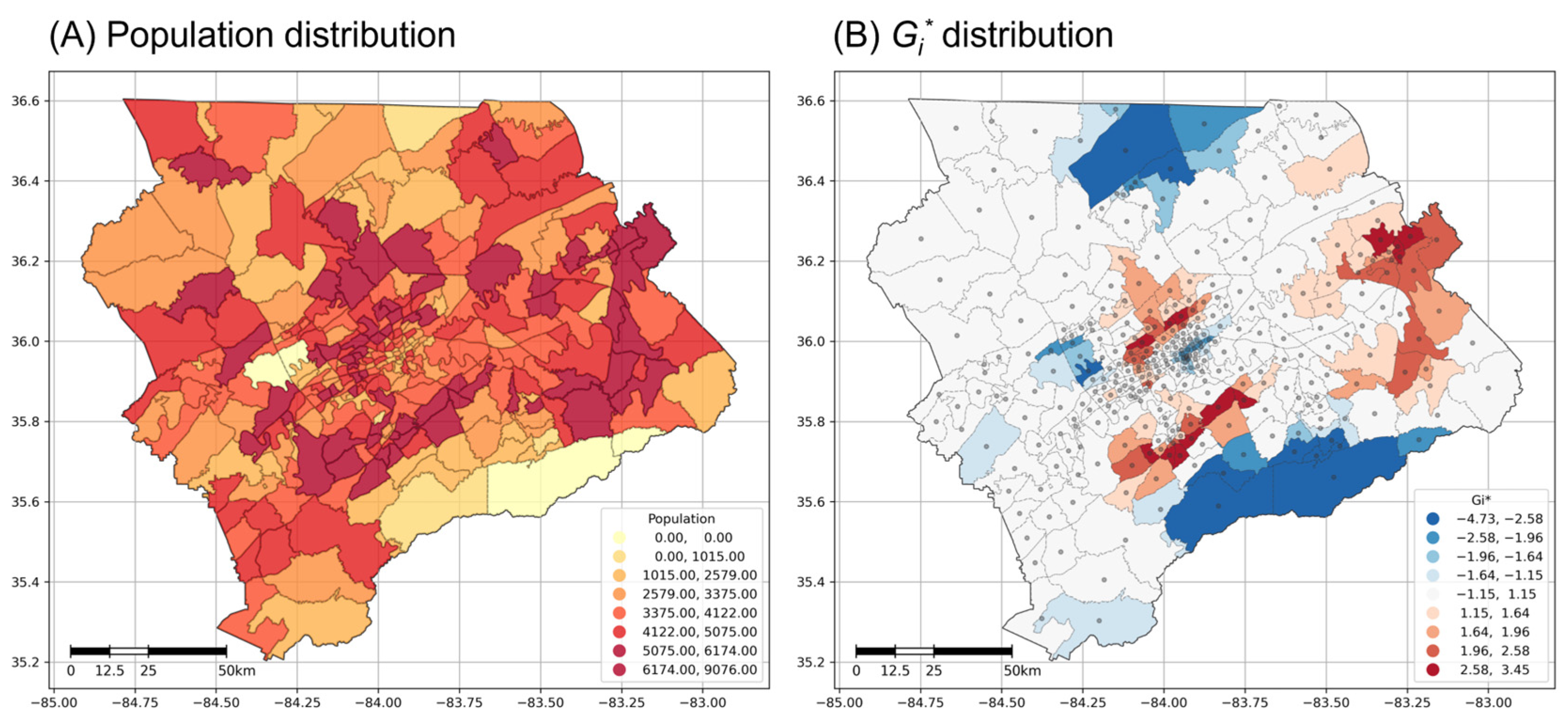
As presented in Figure 1, this research uses the East Tennessee Region as a case study area, planning on the arrangement of waste-collection facilities with a consideration of population distribution [42]. The East Tennessee Region consists of 16 counties and 318 census tracts and the centroids for the census tracts are used as both demand nodes and candidate facility sites. Population data for the census tracts based on the 2020 Census is used as the weights of the models. Figure 4 illustrates the population distribution by tract for the East Tennessee Region (Figure 4A) and their Gi* distribution (Figure 4B) based on population attributes. The region has a positive autocorrelation for the population distribution, which has a global Moran’s I value of 0.2498 (p-value < 0.0001). The Gi* map (Figure 4B) demonstrates that there are three hot spots and four cold spots in this region. The shape and population distribution of the region are well-suited to investigating the location–allocation behaviors of the proposed model, as it is an evenly bounded quadrangle. Using the East Tennessee Region data, the issue of concern in this region is the arrangement of landfills, which need to be located in this region, and thus dispersion-type spatial optimization models are suggested to provide planning scenarios. All instances included in the numerical experiments using SI-OBNOX models were solved using the commercial solver ILOG CPLEX 12.8 on an Intel Core i7-4790 3.60GHz machine with 16 GB of RAM with optimality.

5. Results

5.1. Location–Allocation Behaviors

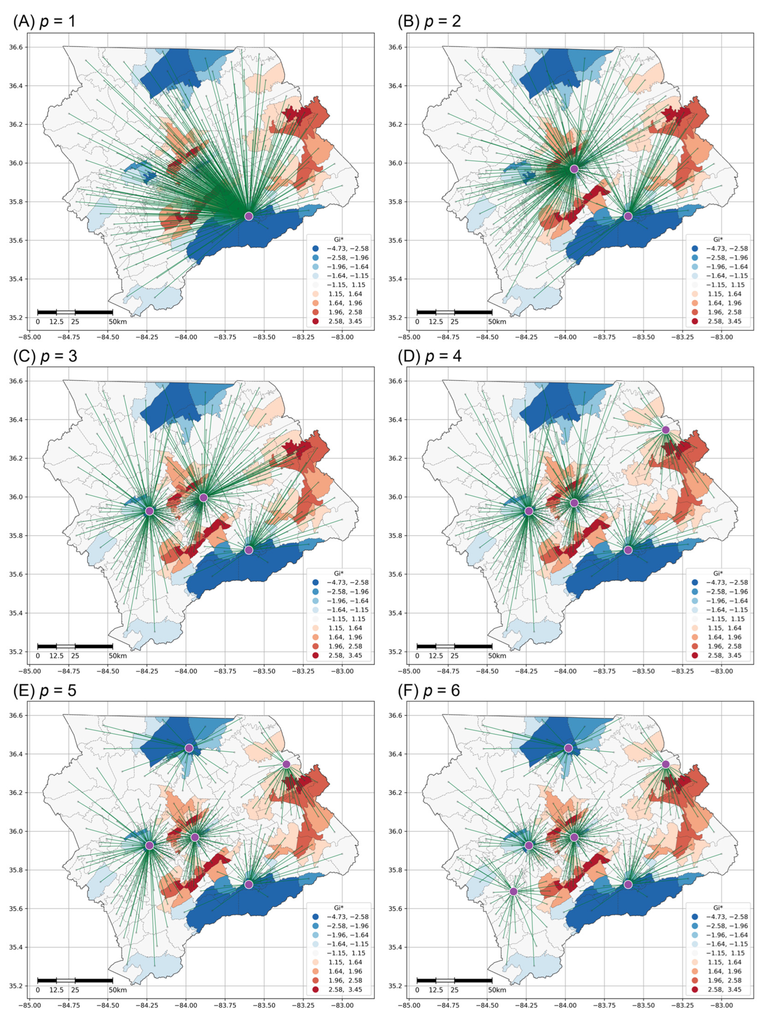
Figure 5 illustrates the optimal spatial arrangements of the obnoxious facilities solved by the SI-OBNOX model for p = 1–6 at a zero-tolerance level (ε = 0). At p = 1 (Figure 5A), the optimal location of the facility is in the southeastern part of the region, where the population is very small, as indicated by low Gi* values. For p = 2 (Figure 5B), the additional facility is placed at the center of the region, which exhibits relatively low Gi* values (see Figure 4B for the Gi* distribution). This outcome aligns with the behavior of traditional OFLPs. However, as the value of p increases, the spatial arrangement of facilities tends to avoid the areas with large populations and locate the rest of the facilities at the census tracts reflecting the pattern of the Gi* values. This strongly indicates that the SI-OBNOX model effectively maintains its intended behavior, ensuring adequate separation among facilities while also considering proximity to residential areas.
A visual inspection of the location–allocation behaviors illustrates the advantages of the SI-OBNOX model. It demonstrates improved spatial arrangements of facilities, making it a more effective decision-support tool for obnoxious facility planning. Compared to Figure 1 in Section 2, the unique location–allocation behavior of the SI-OBNOX model should be noted. Traditional classes of OFLPs display often unrealistic spatial arrangements of optimal location which are unsuitable for effective obnoxious facility planning because most facilities in their models tend to be located at the extreme edges of the region, which is strongly bounded by the boundaries of the region. Differing from the traditional OFLPs, the SI-OBNOX model avoids locating the selected facilities at the extreme peripheries of the research space; instead, the SI-OBNOX model locates facilities relatively close to dense population areas but still avoids the centers of these areas thanks to the SI-constraints. Notably, particularly when compared to the p-obnoxious problem, the SI-OBNOX model achieves a more balanced distribution of facilities across space, taking population distribution into account simultaneously. Figure 5D–F clearly show how the outcome from the SI-OBNOX follows the principles of obnoxious facility location planning in the East Tennessee Region.

5.2. Model Behavior Tuning: Changing Tolerance Standards

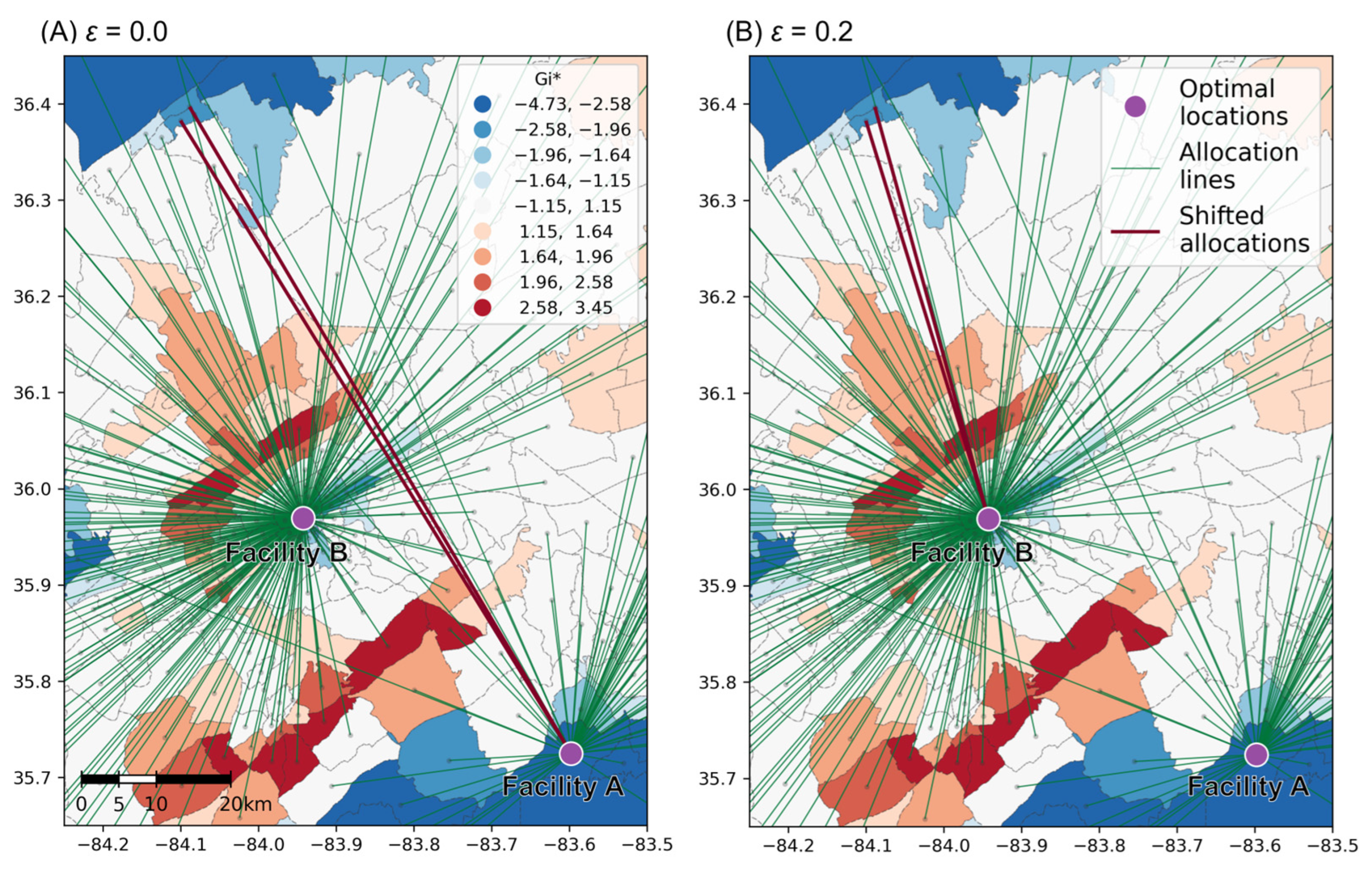
As the tolerance standard ε is equal to 0, all demand nodes should be strictly allocated to the facility site that has a smaller Gi* value than them. So, a few demand nodes are allocated to the open facility that is not nearest to it (See Figure 5B,C). By increasing ε, the restricted allocation behaviors with the low Gi* values furnished by spatially informed constraints are incrementally relieved. Based on other location perspectives, increasing the tolerance standard ε means that the role of the spatial information with Gi* is weakened, and the model behavior of the SI-OBNOX follows that of the p-median problem. Figure 6 illustrates the different allocation behaviors of the SI-OBNOX model with different values of ε (ε = 0 vs. ε = 0.2). As the tolerance standard is relaxed (Figure 6B), a few demand nodes are allocated to their nearest facility. Figure 6 highlights allocation lines with a dark red color. The allocation of those nodes is shifted from facility A (at the lower right corner) to facility B (at the center of the figure). By tuning the tolerance standard, the allocation behavior is affected, improving the objective value of the model.
One of the key benefits of using ε in the SI-OBNOX model is highlighted in Figure 7. As the value of ε increases, the objective value of the model decreases and eventually converges to the objective value of the p-median problem when p = 2. This result is consistently observed across different p levels, indicating that SI-OBNOX effectively mitigates the potential extreme outcomes inherent in OFLPs while significantly improving efficiency in facility arrangement from an economic perspective (i.e., objective value). Consequently, controlling the tolerance standard provides valuable decision-support information for spatial planners, helping them to determine an optimal spatial arrangement for obnoxious facilities based on the level of negative impact on other obnoxious facilities and residential areas.

5.3. Comparison to Other OFLPs

The performance of the spatial arrangement of the model can be assessed in various ways [43]. In this section, to evaluate the performance of the SI-OBNOX model in relation to the families of OFLPs from the perspective of obnoxious facility planning, three indices are introduced: the spatial separation condition (SSC), the spatial externality condition (SEC), and the spatial proximity condition (SPC). Using these indices, the performance of the SI-OBNOX model is compared with other classical OFLP models, including the p-obnoxious, p-dispersion, maxisum dispersion, and MILP models, to quantify how effectively the models satisfy the conditions of obnoxious facility location. These models were selected for comparison because each model exhibits unique and distinct location behaviors, enabling an effective evaluation. Additionally, the results of the p-median model are included because the SI-OBNOX model is based on the structure of the p-median problem. Three indices correspond to key obnoxious facility location conditions and are formally represented through mathematical formulations that incorporate the decision variables and parameters of the proposed model, as detailed below.
SSC :       [ j J min i I d i j Y i Y j ] / p
SEC :       j J h j Y j
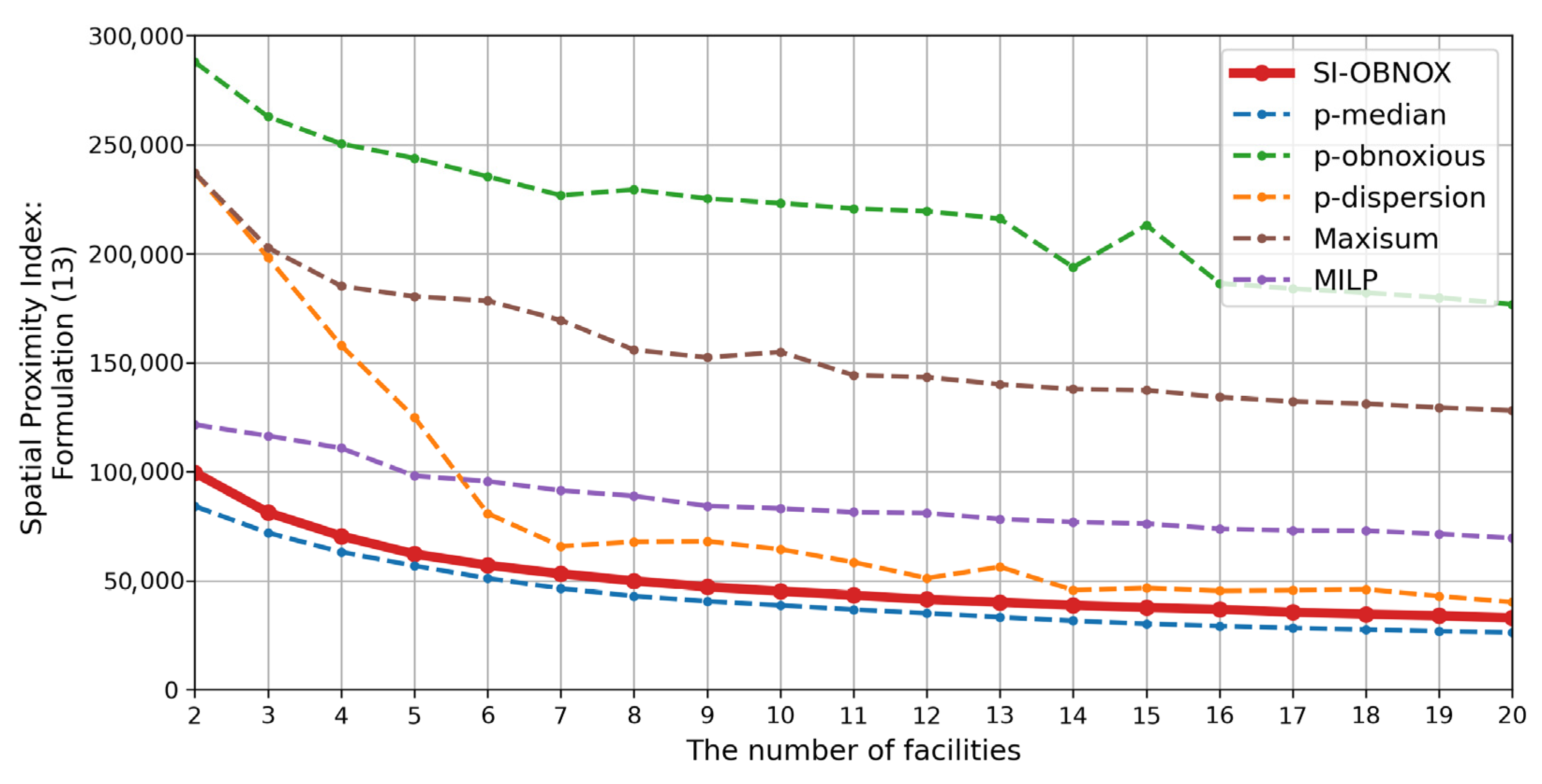
SPC :       ( j J i I d i j X i j ) / n
Formulation (11) represents the average minimum separation distance between each selected facility and its nearest selected facility. This corresponds to the first condition, the spatial separation condition, which ensures that obnoxious facilities are located as far apart from each other as possible. Formulation (12) calculates the total population at the selected facility locations, aligning with the spatial externality condition, which seeks to avoid densely populated areas when siting obnoxious facilities. In our case study, as the centroids of census tracts serve as both demand nodes and candidate sites, the total population at the selected nodes acts as a proxy for the population exposed to the negative externalities of obnoxious facilities. Finally, formulation (13) represents the average distance between selected facilities and demand nodes, corresponding to the spatial proximity condition, which ensures that facilities are located within a reasonable distance from demand nodes for efficient service provision. Figure 8 visually illustrates how each of these conditions is incorporated into the solution.
Three indices are calculated for each obnoxious facility location model by different number of facilities (p = 2 to 20). For models such as p-dispersion and maxisum dispersion, which do not inherently include allocation in their results, this research assumes that demand nodes are allocated to the nearest selected facility. Note that certain models, such as p-obnoxious, p-dispersion, and maxisum dispersion, are challenging to solve within a reasonable timeframe using an exact solution approach (i.e., branch-and-cut algorithm). Therefore, the simulated annealing (SA) algorithm, which is a widely used meta-heuristic approach for solving dispersion-based problems [44,45], is applied to solve these problems if the exact solution approach cannot yield the optimal objective value in a limited timeframe (3 h; 10,800 s).

5.3.1. Spatial Separation Condition (SSC)

Figure 9 shows the change in the value of the SSC index for six selected spatial optimization models. As the SSC index measures the level of negative interactions among obnoxious facilities based on distance, a larger value of the index implies better spatial arrangement for obnoxious facility locations. As a note, the highest upper bound (p-dispersion) and the lowest bound (p-obnoxious) represent extreme outcomes that should be avoided in practical planning implementation. The SI-OBNOX model consistently demonstrates reasonable performance across all values of p, making it a reliable approach for obnoxious facility planning. Due to its structural similarity to the p-median model, the SI-OBNOX model follows a trajectory comparable to the p-median case (blue line). However, the p-obnoxious model (green line) performs the worst across all values of p due to its tendency to cluster facility locations. The p-dispersion model (orange line) achieves the best results, as its primary objective is to maximize the minimum separation distance among facilities. The maxisum dispersion model (brown line) performs well for a smaller number of facilities (p ≤ 5) but quickly deteriorates as the value of p increases, ultimately underperforming compared to the SI-OBNOX model. Finally, MILP (purple line) exhibits worse performance than the SI-OBNOX model for most values of p because it does not account for distances between selected facilities at all.

5.3.2. Spatial Externality Condition (SEC)

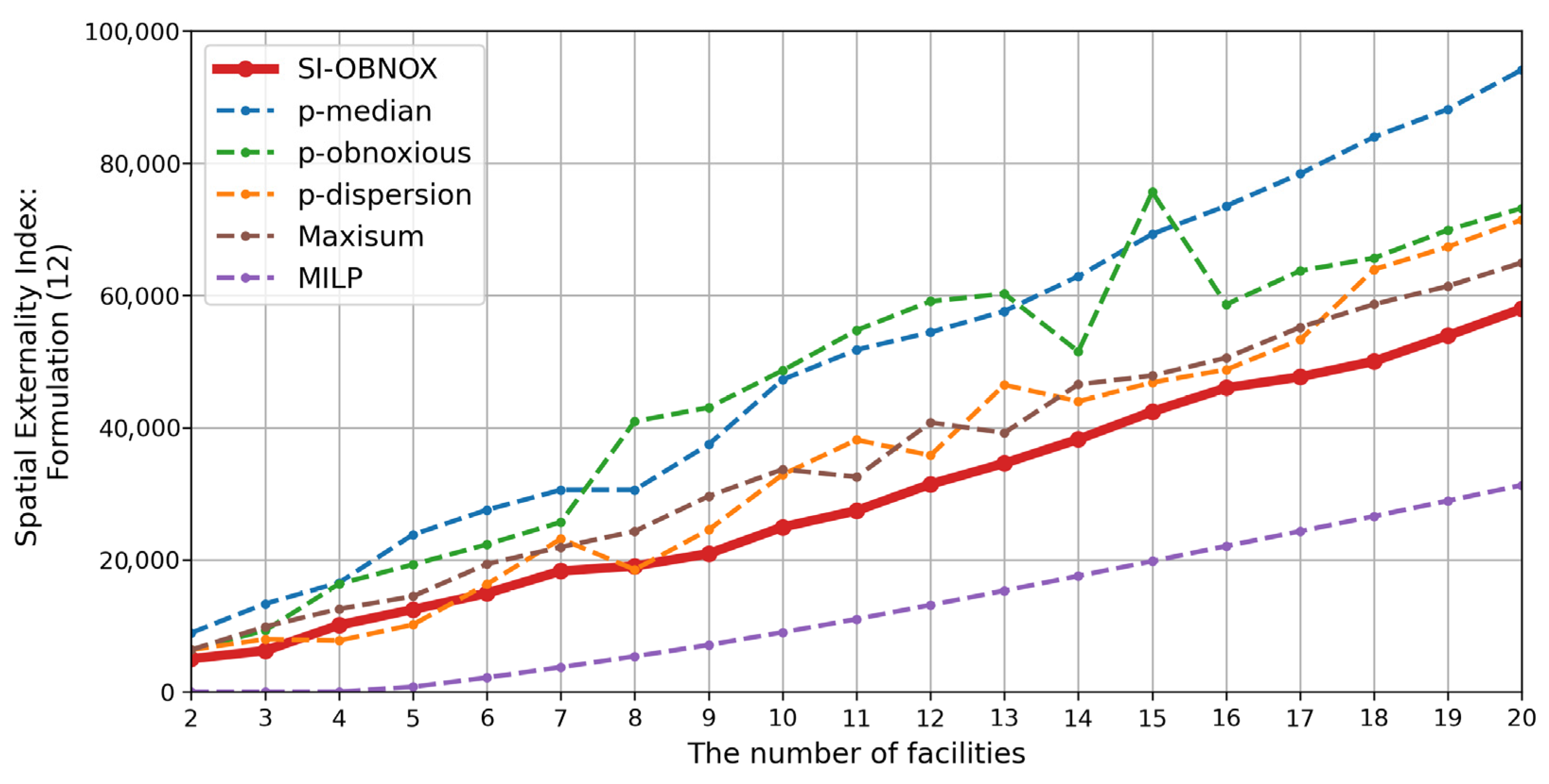
Figure 10 displays the change in the value of the SEC index. In contrast to the spatial separation index, smaller values of the spatial externality index indicate better model performance with smaller externalities to the surrounding areas. The SI-OBNOX model (red line) consistently exhibits a relatively smaller population at the selected facilities for every facility quantity compared to other model results. This indicates that the SI-OBNOX model places facilities in locations that minimize their impact on nearby populations thanks to the SI-constraints. The other obnoxious facility location models such as p-dispersion and maxisum dispersion do not explicitly account for population distribution, leading to unpredictable spatial externality index values as p changes. While the p-obnoxious model incorporates population attributes, its location behavior does not effectively reflect the spatial distribution of populations. Conversely, the MILP model, which explicitly minimizes the population affected by the negative impact of obnoxious facilities, performs best in terms of the spatial externality condition (SEC). However, its performance in the next aspect, SPC, remains less competitive in comparison.

5.3.3. Spatial Proximity Condition (SPC)

Figure 11 illustrates the change in the value of the SPC index, which measures the distance between selected facilities and demand nodes. Although obnoxious facilities negatively impact their surroundings, they must remain reasonably close to demand nodes to maintain system efficiency. Lower values of the spatial proximity index indicate better performance in balancing negative impact reduction with efficient service provision. The SI-OBNOX model achieves better spatial proximity to demand nodes compared to all other obnoxious facility location models. Its performance is very close to that of the p-median model, demonstrating the SI-OBNOX model’s ability to simultaneously minimize negative impacts on neighborhoods while ensuring efficient service delivery. Among the obnoxious facility location models, the p-dispersion model performs relatively well due to the regular distribution of selected facilities driven by its objective function.

6. Discussion

6.1. Location Behaviors of the Models

Visual inspection of the spatial arrangement of the selected facilities may help planners to understand the implications of the three indices more precisely. Figure 12 illustrates the spatial arrangement of the optimal location of each model when p = 7, which is chosen because it effectively highlights the differences among models for all three indices. First, the spatial arrangement of the optimal location under the SI-OBNOX model in Figure 12A should be compared with Figure 12F, the case of the p-median problem. The spatial pattern of the facilities is similar between the two models. However, the SI-OBNOX model explicitly avoids locating facilities in densely populated areas (represented by red colors with high Gi* values), whereas the p-median model tends to locate facilities in high-density residential areas, which may lead to negative impacts on communities, despite maintaining efficient service provision.
Considering the result of the SI-OBNOX model (Figure 12A), the p-obnoxious model (Figure 12B) results in a highly clustered spatial arrangement, with most facilities concentrated in the northwest corner of the region. While demand nodes are allocated to their closest facility, the overall system efficiency is compromised. Many of the selected facilities fail to allocate any demand nodes, rendering them redundant. Consequently, the p-obnoxious model performs poorly across all three indices and is not suitable for practical planning purposes. The p-dispersion model (Figure 12C) locates the selected facilities regularly across the region, thus effectively minimizing the negative interactions among facilities. However, as highlighted in red arrows, the p-dispersion model does not account for the spatial distribution of the population, resulting in some facilities being located in densely populated areas. Compared to the SI-OBNOX model, the p-dispersion model ensures sufficient separation distance among facilities; however, it fails to adequately address the negative impacts on the surrounding communities of selected facilities. Similarly to the p-dispersion model, the maxisum dispersion model (Figure 12D) prioritizes maximizing facility separation. However, local clusters of facilities are observed in peripheral areas, highlighted by red circles. So, the p-dispersion model may be effective in scenarios when the population distribution is not a key factor when making a planning decision, and maxisum dispersion model may struggle to consider interactions among facilities and the spatial distribution of populations effectively. Finally, the MILP model (Figure 12E) places facilities in sparsely populated areas, aligning closely with the population distribution. Its explicit objective of minimizing the total population affected by obnoxious facilities ensures effective performance in terms of spatial externality. However, the MILP model does not consider interactions among facilities, leading to local clusters, such as one in the southeast part of the region. This clustering may be problematic if facility separation is a priority in planning decisions.
Based on the comparisons between the SI-OBNOX model and existing OFLPs, the results clearly presents that the spatially informed constraint effectively controls the location behavior of the optimal solution, thereby improving the efficiency of decision-making for obnoxious facility siting while reducing negative impacts on residential neighborhoods, strongly indicating that the SI-OBNOX model can serve as a valuable tool for planners seeking to avoid extreme or impractical spatial arrangements when designing obnoxious facility systems.

6.2. Computational Efficiency and Scalability

The computational efficiency of the SI-OBNOX model should be compared with the existing OFLP family. As summarized in Table A1, the SI-OBNOX model significantly outperforms most of the existing OFLPs in terms of computational efficiency, except for the MILP model, despite the gaps being marginal. In particular, the computational performance of the p-obnoxious, p-dispersion, and maxisum dispersion models is substantially inferior to that of the SI-OBNOX model for all p. These findings highlight the superior computational efficiency and scalability of the SI-OBNOX model compared to other OFLPs, indicating its potential applicability to larger-scale regional planning problems.
Notably, the SI-OBNOX model consistently outperforms the p-obnoxious model across all instances, even though both are based on the model structure of the p-median problem. The performance gap between the two is significant: the SI-OBNOX model solves all instances in under 5 s, whereas the p-obnoxious model requires extensive amount of solution time for even the smallest instances. This implies that the spatially informed constraints in the SI-OBNOX model effectively improve spatial arrangement for obnoxious facility location without compromising computational performance, while the additional constraints in the p-obnoxious model severely deteriorate its computational efficiency.
Lastly, the MILP model seems to outperform the SI-OBNOX model. However, the difference is minimal, with both models solving all instances in under 5 s, which is substantially marginal (the worst-case solution time is 4.23 s for the SI-OBNOX model with p = 6, as shown in Table A1). Rather, as noted in the previous section, the spatial configurations resulting from the MILP model are often impractical for real-world planning applications, especially in terms of negative interaction between facilities. In contrast, the SI-OBNOX model offers more realistic and actionable planning outcomes, which proves the comprehensive outperformance of the proposed model in terms of both computational efficiency and solution quality.

7. Conclusions

This research introduces the SI-OBNOX model, an alternative location model for obnoxious facilities based on a spatially informed optimization approach using SI-constraints. The SI-OBNOX model provides a more realistic spatial arrangement of selected facilities compared to other OFLPs, achieving better outcomes for three critical conditions essential in obnoxious facility location planning. The SI-OBNOX model demonstrates that a spatially informed approach effectively incorporates specific conditions into the modeling objective, offering a reasonable alternative for dispersion modeling, which is the case for solving OFLPs. Specifically, the proposed SI-constraint plays an important role in forcing the model to locate facilities near populated areas to improve the service provision efficiency at the same time as retaining a certain standard of proximity to the centers of densely populated areas to avoid negative externalities by leveraging additional spatial characteristics from the spatial statistical measurement. The results indicate that the SI-OBNOX model outperforms existing OFLPs in terms of both solution quality for spatial arrangement and computational efficiency.
Although the SI-OBNOX model with SI-constraints effectively improves the solution quality of the obnoxious facility location problems, the effectiveness of these constraints may diminish when the demand surface exhibits little spatial autocorrelation. In other words, if demand weights are randomly or uniformly distributed across the planning region—though it is unlikely to occur—the SI-constraints no longer regulate the model behaviors. Therefore, when applying SI-constraints to location–allocation problems, the presence of spatial autocorrelation should be examined a priori.
This research also provides a systematic yet thorough comparison of location behaviors across various OFLPs. To the best of our knowledge, while many previous studies have addressed the location of obnoxious facilities, few have analyzed the actual spatial behavior of these models. The analytical results produced in this study serve as a foundation for future research aimed at improving obnoxious facility location models, as well as other location–allocation type spatial problems. As a future direction, the SI-OBNOX model could incorporate environmental factors, which are essential for achieving sustainable facility location planning. Additionally, spatial optimization modeling can be further developed to enhance practical models that reflect real-world characteristics. In particular, in the era of emerging GeoAI, state-of-the-art machine learning (ML) and deep learning (DL) algorithms hold a potentiality for solving large-scale and complex spatial optimization problems. Applying ML/DL approaches to OFLPs represents a promising direction for future research based on our modeling approach.

Author Contributions

Conceptualization, Changwha Oh and Hyun Kim; methodology, Changwha Oh; software, Changwha Oh; validation, Changwha Oh and Hyun Kim; formal analysis, Changwha Oh; investigation, Changwha Oh; resources, Changwha Oh and Hyun Kim; data curation, Changwha Oh; writing—original draft preparation, Changwha Oh; writing—review and editing, Changwha Oh and Hyun Kim; visualization, Changwha Oh; supervision, Hyun Kim; project administration, Hyun Kim; funding acquisition, Hyun Kim. All authors have read and agreed to the published version of the manuscript.

Funding

This research was supported by the National Science Foundation (BCS-1951344). Any opinions, findings, and conclusions or recommendations expressed in this article are those of the authors, and do not necessarily reflect the views of the National Science Foundation.

Data Availability Statement

The raw data supporting the conclusions of this article will be made available by the authors on request.

Acknowledgments

The authors appreciate the staff at the ETDD (East Tennessee Development District) for providing access to the data used in this study and valuable consultation. Their support has been highly valued.

Conflicts of Interest

The authors declare no conflict of interest.

Appendix A

Table A1. Comparison of computational performance among the OFLP models.
pSI-OBNOXp-ObnoxiousMILP
Branch and Cut (B&C)Simulated Annealing (SA)
Sol. Time (s)IterationSol. Time (s)IterationSol. Time (s)Gap (%) Sol. Time (s)Iteration
22.7212,1872321.19185,436--0.03198
32.4410,97410,800.25 *748,53869.012.720.02198
42.08760410,800.23 *566,05995.878.700.02231
52.2753710,800.2 *626,730100.997.640.03228
64.2314,61810,800.17 *524,06595.0610.280.03246
72.13639610,800.17 *519,486129.3019.190.03254
81.98497210,800.16 *591,790133.526.470.03251
92463810,800.17 *623,192136.2019.670.02260
102.03465010,800.19 *579,201132.8810.710.02278
111.78404610,800.38 *515,330152.2335.860.03284
121.69349110,800.17 *512,387123.5040.250.03289
131.66331710,800.23 *495,005147.5937.890.01308
141.63313910,800.23 *509,143133.2238.500.02307
151.61291210,800.2 *501,082148.6447.770.02304
161.86294210,800.25 *501,635140.3539.050.03299
171.89269810,800.19 *469,203144.1737.170.03310
181.97273510,800.25 *472,564138.799.710.03301
191.51246110,800.08 *536,323193.0037.810.02326
201.61239210,800.17 *570,854163.3035.480.03333
pp-DispersionMaxisum Dispersion
B&CSimulated Annealing (SA)B&CSimulated Annealing (SA)
Sol. Time (s)IterationSol. Time (s)Gap (%) Sol. Time (s)IterationSol. Time (s)Gap (%)
212.86728--6582.235,878,689--
326.5941,156--10,800.02 *7,822,1585.7113.50
440.5947,142--10,800.03 *3,638,5666.8927.75
5112.99161,266--10,800.06 *4,897,57010.778.14
6203.11350,371--10,800.03 *4,760,83811.4515.48
71668.441,699,848--10,800.06 *4,981,57512.0212.67
8248.59228,699--10,800.34 *4,765,97813.6818.67
910,800.02 *11,358,96520.910.0010,800.03 *4,764,63017.0221.58
108314.198,966,400--10,800.13 *4,793,78917.8237.27
11619.03595,40721.94−1.4710,800.03 *4,941,57821.1430.59
1210,800.02 *12,068,518--10,800.03 *4,828,13722.2330.18
1310,800.05 *9,359,40826.29−2.2010,800.03 *5,353,20723.8531.88
1410,800.02 *9,449,20231.80−2.3010,800.03 *4,772,81327.9934.48
1510,800.05 *7,340,70537.27−0.6210,800.06 *5,135,70829.5212.25
1610,800.02 *8,917,91634.76−1.2610,800.05 *5,200,46430.7419.95
1710,800.03 *8,261,90233.75−3.2810,800.06 *4,903,94234.2730.16
1810,800.03 *8,279,50834.12−3.9210,800.03 *5,004,86938.8037.76
1910,800.03 *7,338,85343.03−1.9710,800.03 *5,093,32143.7832.58
Gap = (SA−B&C)/B&C * 100, where SA: the best solution yielded by SA algorithm; B&C: the best incumbent solution in B&C at the time of termination. * The B&C algorithm was not able to obtain an optimal solution within 3 h (10,800 s) time limit.

References

  1. Erkut, E.; Karagiannidis, A.; Perkoulidis, G.; Tjandra, S.A. A multicriteria facility location model for municipal solid waste management in North Greece. Eur. J. Oper. Res. 2008, 187, 1402–1421. [Google Scholar] [CrossRef]
  2. Tirkolaee, E.B.; Mahdavi, I.; Esfahani, M.M.S.; Weber, G.W. A robust green location-allocation-inventory problem to design an urban waste management system under uncertainty. Waste Manag. 2020, 102, 340–350. [Google Scholar] [CrossRef]
  3. Santos-Peñate, D.R.; Suárez-Vega, R.R.; de la Nuez, C.F. A Location-allocation Model for Bio-waste Management in the Hospitality Sector. Netw. Spat. Econ. 2023, 23, 611–639. [Google Scholar] [CrossRef]
  4. Cassola, F.; Burlando, M.; Antonelli, M.; Ratto, C.F. Optimization of the regional spatial distribution of wind power plants to minimize the variability of wind energy input into power supply systems. J. Appl. Meteorol. Climatol. 2008, 47, 3099–3116. [Google Scholar] [CrossRef]
  5. Idris, M.N.M.; Hashim, H.; Razak, N.H. Spatial optimisation of oil palm biomass co-firing for emissions reduction in coal-fired power plant. J. Clean. Prod. 2018, 172, 3428–3447. [Google Scholar] [CrossRef]
  6. Austin, M.; Smith, T.E.; Wolpert, J. The Implementation of Controversial Facility-Complex Programs. Geogr. Anal. 1970, 2, 315–329. [Google Scholar] [CrossRef]
  7. Mumphrey, A.J.; Seley, J.E.; Wolpert, J. A decision model for locating controversial facilities. J. Am. Inst. Plan. 1971, 37, 397–402. [Google Scholar] [CrossRef]
  8. Mumphrey, A.J.; Wolpert, J. Equity considerations and concessions in the siting of public facilities. Econ. Geogr. 1973, 49, 109–121. [Google Scholar] [CrossRef]
  9. Church, R.L.; Drezner, Z. Review of obnoxious facilities location problems. Comput. Oper. Res. 2022, 138, 105468. [Google Scholar] [CrossRef]
  10. Hosseini, S.; Esfahani, A.M. Obnoxious facility location. In Facility Location: Concepts, Models, Algorithms and Case Studies; 2009; pp. 315–345. [Google Scholar]
  11. Griffith, D.A.; Chun, Y.; Kim, H. Spatial autocorrelation informed approaches to solving location–allocation problems. Spat. Stat. 2022, 50, 100612. [Google Scholar] [CrossRef]
  12. Griffith, D.A.; Chun, Y.; Kim, H. The majority theorem for the single (p = 1) median problem and local spatial autocorrelation. Geogr. Anal. 2023, 55, 107–124. [Google Scholar] [CrossRef]
  13. Oh, C.; Kim, H.; Chun, Y. An Efficient Solving Approach for the p-Dispersion Problem Based on the Distance-Based Spatially Informed Property. Geogr. Anal. 2024, 56, 600–623. [Google Scholar] [CrossRef]
  14. Oh, C.; Kim, H.; Chun, Y. An Efficient Approach for Solving Hub Location Problems Using Network Autocorrelation Structures. Ann. Am. Assoc. Geogr. 2025, 115, 1263–1285. [Google Scholar] [CrossRef]
  15. Shier, D.R. A min-max theorem for p-center problems on a tree. Transp. Sci. 1977, 11, 243–252. [Google Scholar] [CrossRef]
  16. Kuby, M.J. Programming models for facility dispersion: The p-dispersion and maxisum dispersion problems. Geogr. Anal. 1987, 19, 315–329. [Google Scholar] [CrossRef]
  17. Moon, I. Application of graph theory to a location problem. In Proceedings of the Joint National Meeting of ORSA/TIMS, Atlanta, GA, USA, 7–9 November 1977. [Google Scholar]
  18. Moon, I.D.; Chaudhry, S.S. An analysis of network location problems with distance constraints. Manag. Sci. 1984, 30, 290–307. [Google Scholar] [CrossRef]
  19. Erkut, E.; ReVelle, C.; Ülküsal, Y. Integer-friendly formulations for the r-separation problem. Eur. J. Oper. Res. 1996, 92, 342–351. [Google Scholar] [CrossRef]
  20. Erkut, E.; Neuman, S. Comparison of four models for dispersing facilities. INFOR Inf. Syst. Oper. Res. 1991, 29, 68–86. [Google Scholar] [CrossRef]
  21. Oh, C.; Chun, Y.; Kim, H. Location planning of emergency medical facilities using the p-dispersed-median modeling approach. ISPRS Int. J. Geo-Inf. 2023, 12, 497. [Google Scholar] [CrossRef]
  22. Lei, T.L.; Church, R.L. A unified model for dispersing facilities. Geogr. Anal. 2013, 45, 401–418. [Google Scholar] [CrossRef]
  23. Murray, A.T.; Church, R.L. Solving the anti-covering location problem using Lagrangian relaxation. Comput. Oper. Res. 1997, 24, 127–140. [Google Scholar] [CrossRef]
  24. Murray, A.T.; Church, R.L. Facets for node packing. Eur. J. Oper. Res. 1997, 101, 598–608. [Google Scholar] [CrossRef]
  25. Murray, A.T.; Church, R.L. Measuring the efficacy of adjacency constraint structure in forest planning models. Can. J. For. Res. 1995, 25, 1416–1424. [Google Scholar] [CrossRef]
  26. Murray, A.T.; Kim, H. Efficient identification of geographic restriction conditions in anti-covering location models using GIS. Lett. Spat. Resour. Sci. 2008, 1, 159–169. [Google Scholar] [CrossRef]
  27. Niblett, M.R.; Church, R.L. The disruptive anti-covering location problem. Eur. J. Oper. Res. 2015, 247, 764–773. [Google Scholar] [CrossRef]
  28. Church, R.L.; Cohon, J.L. Multiobjective Location Analysis of Regional Energy Facility Siting Problems; No. BNL-50567; Brookhaven National Laboratory. (BNL): Upton, NY, USA, 1976. [Google Scholar]
  29. Daskin, M.S. Network and Discrete Location: Models, Algorithms, and Applications; Wiley: Hoboken, NJ, USA, 1995. [Google Scholar]
  30. Ratick, S.J.; White, A.L. A risk-sharing model for locating noxious facilities. Environ. Plan. B Plan. Des. 1988, 15, 165–179. [Google Scholar] [CrossRef]
  31. Church, R.L.; Murray, A.T. Business Site Selection, Location Analysis, and GIS; Wiley: Hoboken, NJ, USA, 2009. [Google Scholar]
  32. Drezner, T.; Drezner, Z.; Zerom, D. The obnoxious competitive facility location model. Netw. Spat. Econ. 2023, 23, 885–903. [Google Scholar] [CrossRef]
  33. Marsh, M.T.; Schilling, D.A. Equity measurement in facility location analysis: A review and framework. Eur. J. Oper. Res. 1994, 74, 1–17. [Google Scholar] [CrossRef]
  34. Talen, E. Visualizing fairness: Equity maps for planners. J. Am. Plan. Assoc. 1998, 64, 22–38. [Google Scholar] [CrossRef]
  35. Chea, H.; Kim, H. Assessing trauma center accessibility in the Southeastern region of the US to improve healthcare efficacy using an anti-covering approach. PLoS Glob. Public Health 2023, 3, e0002230. [Google Scholar] [CrossRef]
  36. Getis, A.; Ord, J.K. The analysis of spatial association by use of distance statistics. Geogr. Anal. 1992, 24, 189–206. [Google Scholar] [CrossRef]
  37. Ord, J.K.; Getis, A. Local spatial autocorrelation statistics: Distributional issues and an application. Geogr. Anal. 1995, 27, 286–306. [Google Scholar] [CrossRef]
  38. Hakimi, S.L. Optimum locations of switching centers and the absolute centers and medians of a graph. Oper. Res. 1964, 12, 450–459. [Google Scholar] [CrossRef]
  39. Hakimi, S.L. Optimum distribution of switching centers in a communication network and some related graph theoretic problems. Oper. Res. 1965, 13, 462–475. [Google Scholar] [CrossRef]
  40. Balinski, M.L. Integer programming: Methods, uses, computations. Manag. Sci. 1965, 12, 253–313. [Google Scholar] [CrossRef]
  41. Rosing, K.E.; ReVelle, C.S.; Rosing-Vogelaar, H. The p-median and its linear programming relaxation: An approach to large problems. J. Oper. Res. Soc. 1979, 30, 815–823. [Google Scholar] [CrossRef]
  42. East Tennessee Development District. 2024 Annual Report. Available online: https://www.etdd.org/resources/reports/ (accessed on 14 August 2025).
  43. Zhou, E.; Murray, A.T. Facility layout and spatial configuration efficiency assessment. Netw. Spat. Econ. 2024, 25, 487–511. [Google Scholar] [CrossRef]
  44. Johnson, D.S.; Aragon, C.R.; McGeoch, L.A.; Schevon, C. Optimization by simulated annealing: An experimental evaluation; part II, graph coloring and number partitioning. Oper. Res. 1991, 39, 378–406. [Google Scholar] [CrossRef]
  45. Erkut, E.; Ülküsal, Y.; Yenicerioğlu, O. A comparison of p-dispersion heuristics. Comput. Oper. Res. 1994, 21, 1103–1113. [Google Scholar] [CrossRef]
Figure 1. Location (-allocation) behaviors of traditional OFLPs: (A) p-obnoxious, (B) maxisum dispersion, (C) p-dispersion, and (D) MILP (p = 5 case). Blue dots, gray dots, and green lines illustrate the location of facilities, demand nodes, and allocation lines respectively. These maps display the case study area.
Ijgi 14 00449 g001
Figure 2. Flowchart of the research framework for the SI-OBNOX model.
Ijgi 14 00449 g002
Figure 3. Conceptual diagram of the behavioral characteristic of the SI-OBNOX model. Blue dots, black dots, and green lines illustrate the location of facilities, demand nodes, and allocation lines respectively.
Ijgi 14 00449 g003
Figure 4. Spatial characteristics of population in the East Tennessee Region: (A) census-tract-level population distribution; (B) Gi* value distribution based on population. Gray dots in (B) depict centroid of demand units.
Ijgi 14 00449 g004
Figure 5. Spatial arrangements of obnoxious facilities solved by the SI-Obnoxious model (p = 1–6). Purple dots, gray dots, and green lines illustrate the optimal location of facilities, demand nodes, and allocation lines respectively.
Ijgi 14 00449 g005
Figure 6. Comparison of location–allocation behaviors based on different tolerance standard levels: (A) ε = 0.0, (B) ε = 0.2.
Ijgi 14 00449 g006
Figure 7. Change in objective value with different tolerance levels ε. The black dashed horizontal line indicates the optimal value of the p-median problem with the same instance p = 2.
Ijgi 14 00449 g007
Figure 8. Visual illustration of three obnoxious planning-related indices. SSC: Spatial separation condition, SEC: spatial externality condition, SPC: spatial proximity condition. Blue dots, gray dots, and green lines illustrate the location of facilities, demand nodes, and allocation lines respectively.
Ijgi 14 00449 g008
Figure 9. Change in spatial separation index by the number of facilities for each model.
Ijgi 14 00449 g009
Figure 10. Change in spatial externality index by the number of facilities for each model.
Ijgi 14 00449 g010
Figure 11. Change in spatial proximity index by the number of facilities of each model.
Ijgi 14 00449 g011
Figure 12. Comparison of location behaviors among the models: (A) SI-OBNOX model, (B) p-obnoxious, (C) p-dispersion, (D) maxisum dispersion, (E) MILP, and (F) p-median (p = 7 case). Purple dots, gray dots, and green lines illustrate the optimal location of facilities, demand nodes, and allocation lines respectively.
Ijgi 14 00449 g012
Disclaimer/Publisher’s Note: The statements, opinions and data contained in all publications are solely those of the individual author(s) and contributor(s) and not of MDPI and/or the editor(s). MDPI and/or the editor(s) disclaim responsibility for any injury to people or property resulting from any ideas, methods, instructions or products referred to in the content.