Spatio-Temporal Variability and Environmental Associations of Emergency Department Demand: A Longitudinal Analysis in Zaragoza, Spain (2011–2024)

Abstract

Emergency department (ED) overcrowding has become a critical public health issue worldwide, driven by increasing demand and limited healthcare resources. This study analyzes the spatio-temporal variability of ED visits at Royo Villanova Hospital (Zaragoza, Spain) from 2011 to 2024, integrating clinical, demographic, environmental, and socioeconomic data. Using geospatial tools and machine learning models (XGBoost with SHAP interpretation), we identify key patterns in ED demand across time and space. Results show that the hour of the day is the most influential variable across all diagnoses, while temperature, humidity, and air pollutants (NO₂, SO₂, O₃) significantly affect respiratory and injury-related visits. Spatial analysis reveals persistent high-demand clusters in specific health zones, with proximity to the hospital playing a major role. The COVID-19 pandemic caused structural shifts in demand, particularly in pediatric care. Our findings highlight the need for tailored, diagnosis-specific predictive models and support the use of geospatial and environmental data for proactive ED resource planning. This approach enhances the capacity of health systems to anticipate demand surges and allocate resources efficiently.

1. Introduction

The overcrowding of hospital emergency departments (EDs) has emerged as a significant public health issue worldwide in recent decades [1]. The continuous increase in demand, driven by population aging, chronic illnesses, seasonal epidemics, social inequalities, and extreme weather events, combined with the limitations of healthcare resources, has frequently led to the collapse of emergency services. This overcrowding negatively impacts the quality, safety, and efficiency of care, and is associated with delays, medical errors, and increased morbidity and mortality [2,3,4]. Consequently, understanding and anticipating ED demand has become a structural challenge for healthcare systems and a public health priority.

Demand for emergency care varies considerably across both space and time, making longitudinal and geospatial analyses essential. Identifying “where” and “when” demand peaks occur can significantly improve the effectiveness of healthcare responses. Previous studies emphasize that understanding the spatiotemporal distribution of emergencies is crucial for planning timely interventions [5]. Spatiotemporal analyses, which integrate location data with time series, enable the identification of geographic clusters of high demand and critical periods of service pressure, thereby guiding the efficient allocation of medical resources. Moreover, geographic information system (GIS) tools facilitate the visualization of demand “hot spots” and the rapid identification of problematic areas [6,7,8]. The use of standardized diagnostic classifications, such as ICD-9-CM (International Classification of Diseases, 9th Revision, Clinical Modification), ensures consistent categorization of cases across time and location, enhancing the reliability of comparative analyses.

Numerous studies indicate that ED demand is influenced by environmental, demographic, and socioeconomic factors. In the environmental domain, extreme weather conditions (e.g., heatwaves, severe cold) and poor air quality have been shown to increase the frequency of visits [9,10,11]. For example, episodes of heatwaves or pollution often trigger respiratory and cardiovascular exacerbations, explaining part of the observed demand peaks. Demographically, aging populations exhibit consistently higher rates of ED utilization [5]. Socioeconomically, communities with lower income or higher vulnerability tend to experience more frequent or “avoidable” ED visits, reflecting how social inequalities are projected onto healthcare demand [12,13]. Collectively, these findings highlight the importance of integrating demographic, environmental, and socioeconomic determinants into demand analyses.

The increasing availability of geospatial data and GIS tools is particularly relevant to this type of analysis. A geoinformational approach allows overlaying healthcare demand with environmental and demographic variables, revealing territorial patterns that may be obscured in aggregate analyses. The health geography literature identifies GIS as a critical tool for healthcare planning, supporting the mapping of spatial demand distribution, identification of high-frequency “hot spots,” and modeling of relationships between geo-environmental factors and health outcomes [7,8]. Advanced spatial techniques, including spatial statistics, geostatistical interpolation, and spatiotemporal clustering, further enhance predictive models by incorporating the geographic dimension, thereby improving the ability of healthcare systems to anticipate demand changes and respond equitably.

Parallel advances in machine learning have enabled the development of robust and interpretable predictive models. Algorithms such as XGBoost (Extreme Gradient Boosting) have been successfully applied in healthcare to predict costs, utilization frequencies, and clinical risks, due to their capacity to handle heterogeneous, large-scale datasets and nonlinear relationships [14,15]. Interpretability is enhanced by SHAP (SHapley Additive exPlanations), which quantifies the relative importance of each variable and supports evidence-based decision-making in clinical and organizational contexts. Integrating environmental and socioeconomic determinants into predictive models not only improves accuracy but also incorporates structural dimensions reflecting social and territorial inequalities.

In addition to temporal analyses, spatial techniques such as choropleth maps allow the assessment of differences across zones in both the number of ED visits and population-adjusted rates. Incorporating georeferenced demographic data enables evaluation of the relative healthcare burden, revealing potential inequalities in service use that may remain hidden when using absolute figures. By combining longitudinal data, spatial analyses, and machine learning, this study contributes to the development of diagnosis-specific predictive models and provides empirical evidence to support proactive and equitable healthcare planning.

This work focuses on the Zaragoza I Health Area (Aragon, Spain) and analyzes ED demand at the Hospital Royo Villanova between 2011 and 2024. The framework integrates clinical, demographic, environmental, and socioeconomic variables using geospatial techniques and predictive models. Although the study is centered on a specific territory, the proposed methodology is generalizable and adaptable to other healthcare settings, offering potential improvements in emergency service planning and demand forecasting. Building on recent advances in health geography and predictive analytics [7,8,14,15,16], this work contributes to the literature by jointly considering spatiotemporal variability, environmental and socioeconomic determinants, and the integration of geospatial and machine learning methods for healthcare demand analysis.

The study pursues four specific objectives: (i) to characterize the spatiotemporal variability of ED demand in Zaragoza I between 2011 and 2024; (ii) to identify geographic clusters of high and low demand using spatial statistics (Moran’s I, LISA); (iii) to assess the influence of environmental, demographic, and socioeconomic determinants on these patterns; and (iv) to develop predictive models that combine machine learning (XGBoost) with interpretable techniques (SHAP) to generate actionable insights for healthcare planning. These objectives are guided by the following research questions: How does ED demand vary across space and time in Zaragoza I? Which environmental and socioeconomic factors are most strongly associated with demand fluctuations? To what extent can machine learning models enhance anticipation of demand peaks compared to conventional approaches?

The methodological choice of integrating GIS, spatial statistics, and interpretable machine learning is motivated by the need to capture the multidimensional nature of healthcare demand. This combined approach provides both descriptive evidence (spatial and temporal patterns, population-adjusted rates, geographic clusters) and predictive outputs (interpretable models of demand determinants), thereby offering a robust basis for equitable and proactive healthcare resource allocation. As illustrated in Figure 1, the proposed roadmap integrates data preprocessing, spatial analyses, and predictive modeling into a unified framework, advancing both methodological innovation and practical relevance for healthcare planning.

2. Materials and Methods

2.1. Data Structure and Variables

This study utilizes emergency care records from Royo Villanova Hospital (Zaragoza, Spain) spanning from 13 May 2011 to 11 September 2024. The data originate from the hospital information system and include demographic, clinical, and administrative variables for each episode. The geographic scope of analysis corresponds to the Zaragoza I Health Area, which comprises 14 basic health zones (BHZs), for which the hospital serves as the referral center.

The selection of the territorial unit is a critical methodological consideration. In Spain, the BHZ represents the smallest geographic unit employed for healthcare planning [17]. Each BHZ encompasses the population served by a primary care team and serves as the reference for the local organization of healthcare services. Analyzing ED demand at the BHZ level enables the capture of local heterogeneity, facilitates comparisons across equivalent zones, and ensures alignment with the existing care infrastructure. This level of granularity allows for targeted interventions in specific communities and supports the replicability of the approach in other regions with similar territorial units [16].

Following data collection, all records were anonymized to preserve patient confidentiality. Aggregation was performed at multiple temporal levels (hourly, daily, monthly, and yearly) to facilitate analysis and visualization. Two auxiliary .json files were integrated to support categorization and analysis: (i) cie9_data.json, which maps ICD-9-CM codes into broader clinical categories, and (ii) area_sanitaria.json, linking each BHZ to its corresponding Health Area (Zaragoza I, II, or III).

The primary outcome variable is emergency care demand, measured as the number of episodes per time slot (hourly, daily, weekly, or monthly) and per BHZ. This outcome is analyzed in relation to both internal and external explanatory variables, which are integrated through temporal and geospatial linkage.

Explanatory variables are classified into two categories: internal (clinical and demographic) and external (environmental, sociodemographic, socioeconomic, and contextual). External datasets were incorporated to examine associations with ED demand. Specifically, these include climatic variables (mean, maximum, and minimum temperature; relative humidity), air pollutants (PM10, NO₂, O₃), sociodemographic indicators (total population, average age, proportion of population aged ≥65, aging index, dependency rate), socioeconomic indicators (average income, unemployment rate, Gini index, household size, proportion of single-person households), and social context or event-based variables (public holidays and high-attendance events such as football matches, concerts, and popular races). These variables were linked temporally (by date of visit) and spatially (by BHZ) to enable integrated analyses with the emergency department data.

Table 1. Internal variables (Name and Type).

Name	Type
Admission date/time (ingreso_dt)	Date/time
Age (edad)	Numeric
Gender (sexo)	Categorical
Province (provincia)	Categorical
Basic Health Zone (BHZ)	Categorical
Triage level (triaje)	Ordinal (I–V)
Primary diagnosis (diag1_cie_cg)	Categorical
Discharge destination (destino_alta)	Categorical
Destination center (centro_destino)	Categorical
Dates of discharge request and execution (solic_alta_dt, alta_dt)	Date/time

summarizes the internal variables extracted from the HIS, encompassing demographic, clinical, and administrative information that directly characterize each emergency episode.

Table 2. External variables (Name, Type, and Temporal resolution).

Name	Type	Temporal Resolution
Temperature (mean, max, min)	Numeric	Hourly/Daily
Relative humidity	Numeric	Hourly/Daily
Air pollutants (PM10, NO2, O3)	Numeric	Hourly/Daily
Population (by age group)	Numeric	Annual
Aging index, dependency ratio	Numeric	Annual
Income, unemployment rate	Numeric	Annual
Gini index, household size	Numeric	Annual
Public holidays	Binary	Daily
Events (football matches, concerts, festivals)	Binary	Event-based

presents the external variables, including environmental, sociodemographic, and contextual factors linked to BHZs or city-level data, which are used to examine associations with emergency care demand.

Variables were selected based on theoretical relevance, data completeness, and interpretative value. Variables exhibiting low variability, excessive missing data, or high collinearity were excluded to ensure parsimony and robustness in subsequent analyses. While a broader set of variables was explored during preliminary analyses, only those demonstrating significant associations or providing interpretative value are presented in the final results, promoting clarity and scientific rigor.

2.2. Spatial Data and Geographic Units

The territorial unit employed for the geospatial analysis was the BHZ, which constitutes the minimum organizational structure of the Spanish healthcare system [17]. Each BHZ represents a population served by a primary care team and functions as a stable unit for planning and analyzing healthcare activity. Although some BHZs contained fewer than 30 observations, their inclusion is methodologically justified. In health geography, small-area analyses are often necessary to capture local heterogeneity and disparities in service utilization. Recent methodological frameworks, such as the SMART appraisal tool, emphasize the importance of spatial granularity over arbitrary sample size thresholds when the territorial unit is structurally relevant and aligned with healthcare planning [18]. Furthermore, Bayesian spatial models have demonstrated robustness in sparse data contexts, provided that spatial dependence is adequately modeled [19].

While the study includes emergency care data from all BHZs within the Aragon region, the spatial analysis focused on the Zaragoza I Health Area, as the Royo Villanova Hospital serves as its reference center and the majority of episodes originate from this zone. This focus improves visualization, avoids overrepresentation of marginal zones, and maintains coherence with the hospital’s catchment area. Attendances from other BHZs or provinces were considered in global analyses but were not cartographically represented.

To represent the spatial dimension, official shapefiles provided by the Ministry of Health and the Government of Aragon were integrated within a GIS environment, enabling spatial joins and the generation of thematic maps. Population data by BHZ were obtained from annual reports of the Aragonese Institute of Statistics, with the exception of 2023, when disaggregated data were unavailable due to a change in the data storage system.

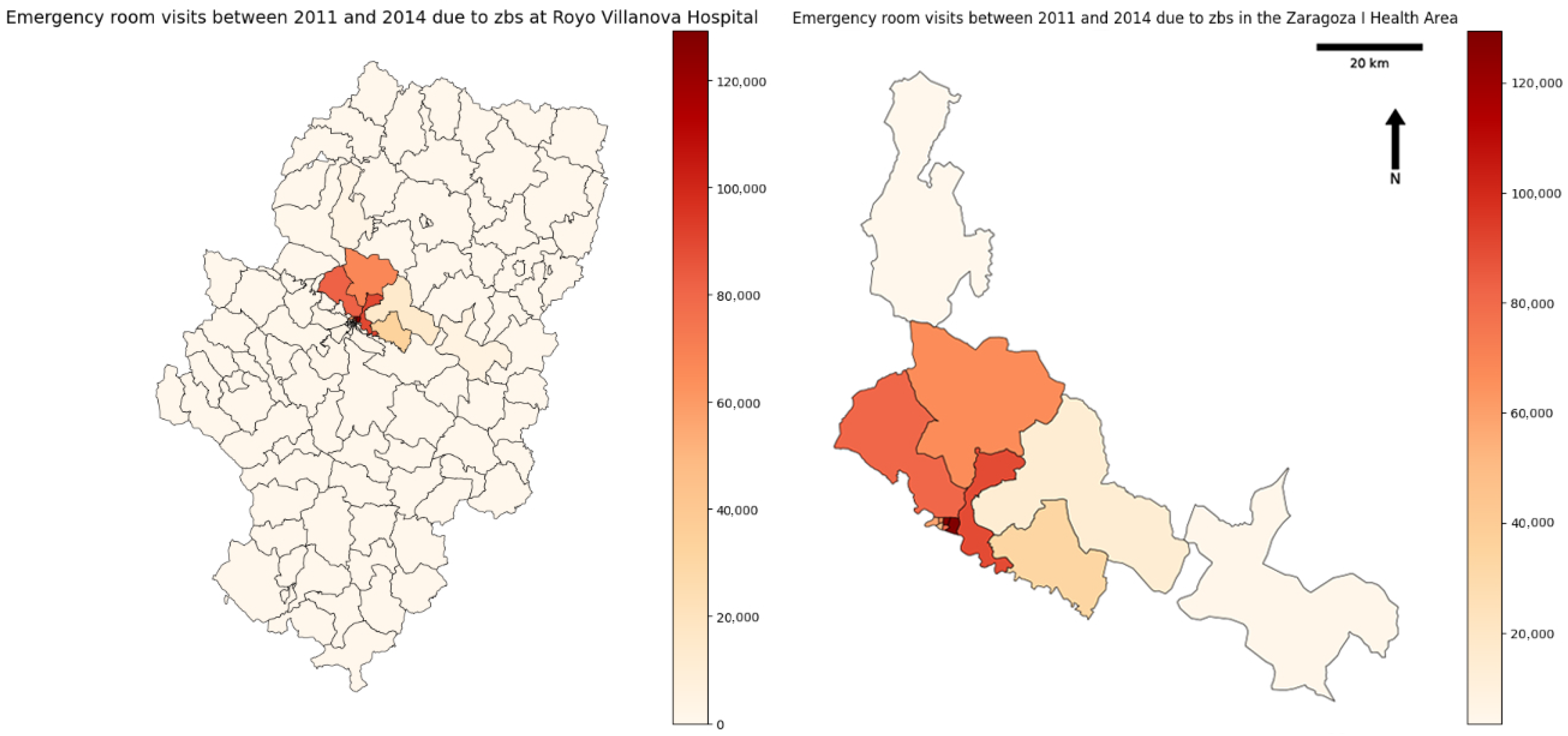
From the georeferenced data, several figures were generated. As illustrated in Figure 2, most recorded attendances in the province are concentrated in BHZs belonging to the Zaragoza I Health Area. Additional supporting figures have been relocated to the Supplementary Figures to improve readability. These include the temporal evolution of emergency care attendance, which highlight a decline beginning in 2020, a stable population trend across BHZs, and attendance rates adjusted per 1000 inhabitants. Notably, higher adjusted rates were observed in rural BHZs near the reference hospital, suggesting a proximity effect on service utilization.

These visualizations facilitated the identification of territorial inequalities, both in absolute terms and relative to population size, highlighting BHZs with high service pressure or mismatches between population and service utilization.

Additionally, population density indicators were calculated as a preliminary step, followed by the application of spatial statistical techniques to explore geographic clusters and local autocorrelation in emergency care utilization patterns, as detailed in Section 3.

2.3. Data Preprocessing

Prior to analysis, the data were structured and aggregated to generate derived variables, standardize information, and adapt it to different temporal resolutions. The preprocessing included the following steps.

2.3.1. Temporal Structuring

Based on the admission date and time variable (ingreso_dt), new variables were derived to enable analysis of demand variability at multiple temporal scales. Specifically, the following time units were created:

• Hour: hour of admission (0–23).
• Day of the week: Monday to Sunday.
• Month of the year: January to December.
• Calendar year: 2011 to 2024.
• Epidemiological week: calendar weeks 1–52.
• PreCOVID/PostCOVID interval: 2011–2019 versus 2021–2024.

These temporal variables enabled the construction of time series at hourly, daily, monthly, and annual levels.

2.3.2. Record Aggregation

The original dataset contained one record per emergency episode. Aggregated time series of attendance frequencies were created across the temporal scales mentioned above, using the number of records per interval as the counting unit. Aggregation was performed both globally and stratified by relevant characteristics such as main diagnosis, gender, age, triage level, and BHZ.

2.3.3. Integration with External Data

Environmental variables (temperature, humidity, air pollutants) with hourly or daily resolution were incorporated by synchronizing them with each episode’s date and time of admission. For these variables, data from the nearest monitoring stations were used.

Additionally, sociodemographic contextual variables (e.g., population by BHZ and year) were integrated to enable frequency normalization and calculation of adjusted attendance rates. Population data for 2023 were unavailable due to a change in the data storage system.

2.4. Predictive Modeling and Evaluation

2.4.1. Model Selection and Justification

Emergency care demand was modeled using XGBoost, a tree-based ensemble algorithm recognized for its capacity to handle large, heterogeneous datasets and capture complex, nonlinear relationships [14,15]. Alternative approaches, including Random Forest and linear regression, ere evaluated during preliminary testing. XGBoost was ultimately selected due to its superior performance, computational efficiency, and ability to capture nonlinear relationships in heterogeneous datasets. This balance between predictive accuracy, robustness, and transparency makes XGBoost particularly suitable for healthcare demand modeling under data constraints.

Since the target variable represents a discrete event count (number of attendances per hour), hyperparameters were adjusted accordingly. Specifically, the model was trained using objective = ’count:poisson’, treating the target as a Poisson-distributed variable appropriate for count data over fixed time intervals. The evaluation metric eval_metric = ’poisson-nloglik’ was chosen to assess model fit based on the negative log-likelihood of the Poisson distribution, offering a more suitable alternative to mean squared error for low-count data. Separate XGBoost models were trained for each diagnostic group, with datasets split into training (80%) and testing (20%) sets. Input features included temporal variables (hour, day, month, year) and, when applicable, external variables (environmental and socioeconomic indicators). No feature standardization was applied, as XGBoost handles numerical data natively. Hyperparameters were manually tuned to balance complexity and generalization, using values such as max_depth = 6, learning_rate = 0.1, and subsample = 0.8.

The first model was trained exclusively with internal temporal variables to establish a baseline and capture nonlinear interactions between temporal components. This baseline facilitates evaluation of the incremental predictive value provided by external variables. Previous studies support the use of similar approaches in healthcare demand forecasting and resource allocation [14,20].

2.4.2. Feature Importance and Interpretability

Feature importance was assessed to identify variables most influential for model predictions, reduce dimensionality, and enhance interpretability. XGBoost provides three internal metrics:

• Gain: the average contribution of a feature to the model’s loss reduction across all splits where it is used; the most informative metric for assessing predictive impact.
• Cover: the number of observations affected by a feature across all decision splits, indicating the breadth of its influence.
• Weight: the frequency with which a feature is used for splitting across all trees, reflecting selection frequency rather than predictive strength.

To complement these metrics, SHAP (SHapley Additive exPlanations) was used to provide theoretically grounded, local explanations of predictions.

Mathematically, SHAP is grounded in cooperative game theory, where each feature i is assigned a Shapley value ${\varphi }_i$ that represents its average marginal contribution to the model output $f\left(x\right)$ across all possible subsets of features $S\subseteq F\setminus \left\{i\right\}$, with F denoting the complete set of features. The Shapley value is defined as

$${\varphi }_i=\sum _{S\subseteq F\setminus \left\{i\right\}}{\displaystyle \frac{\left|S\right|!\left(\right|F|-|S|-1)!}{\left|F\right|!}}\left[f_{S\cup \left\{i\right\}}\left(x_{S\cup \left\{i\right\}}\right)-f_S\left(x_S\right)\right]$$

This formulation guarantees that the sum of all feature contributions equals the difference between the model prediction and its expected value (${\sum }_i{\varphi }_i=f\left(x\right)-E\left[f\left(x\right)\right]$), thereby satisfying the properties of local accuracy, missingness, and consistency. These theoretical properties make SHAP a robust and interpretable framework for feature attribution in complex, nonlinear models such as XGBoost.

At the interpretative level, the global mean of absolute SHAP values reflects each feature’s average contribution across all observations, while local SHAP values identify the factors driving individual predictions.

Values were computed using the TreeExplainer method and visualized with the function shap.summary_plot. Input datasets included temporal variables and, where applicable, external variables. Feature names were standardized in English for consistency in plotting. This approach ensures robust interpretation of feature contributions while accounting for interactions between variables.

2.4.3. Integration of Spatiotemporal Analysis

Spatial statistical techniques were applied to complement predictive modeling. Local Indicators of Spatial Association (LISA) were computed to detect geographic clusters and local autocorrelation in ED demand patterns. While LISA does not directly enhance predictive performance, it provides critical insights for healthcare planning by identifying areas with heightened service pressure or atypical demand patterns.

The combination of XGBoost, SHAP, and complementary spatial statistics facilitates both predictive and interpretative understanding of ED demand, integrating temporal, demographic, environmental, and geographic dimensions. This integrated framework supports evidence-based decision-making and proactive healthcare resource allocation.

3. Results

The analysis was approached from a multiscale perspective, integrating descriptive exploration, correlation analysis, variable importance evaluation, and basic spatial statistics techniques, all supported by empirical evidence extracted from the dataset.

3.1. Temporal Descriptive Analysis

An initial characterization of emergency demand was carried out, considering three dimensions. First, the temporal dimensions (such as hour of the day, day of the week, month, and year) allow for the observation of seasonal patterns and significant variations in emergency department visits at the Royo Villanova Hospital. These variables are key to understanding the behavioral patterns of the patient population and to anticipating demand peaks.

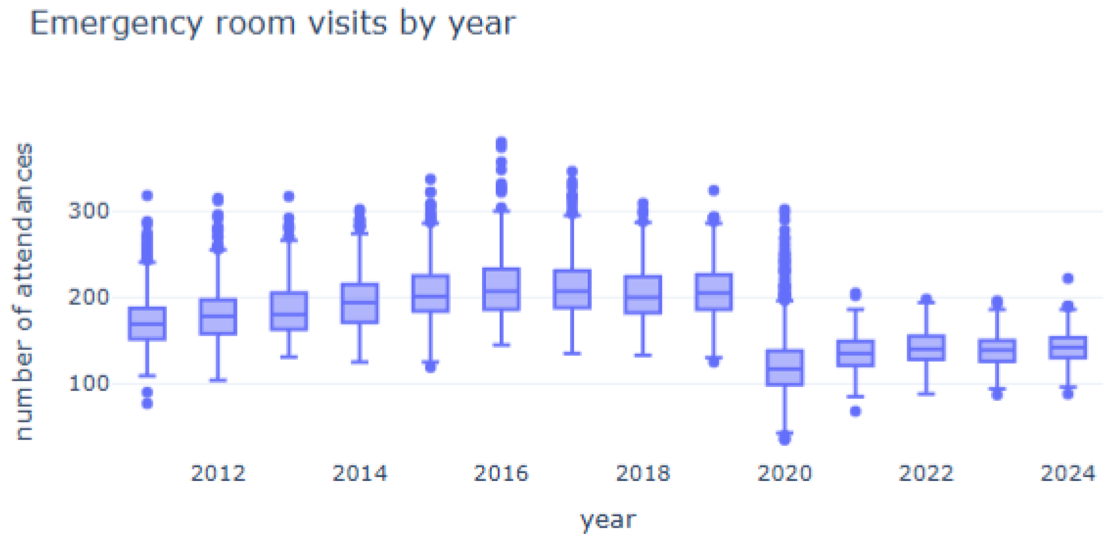
When analyzing data by year, an abrupt change is observed in 2020, coinciding with the onset of the COVID-19 pandemic (Figure 3). This event marks an inflection point in the time series, with a sharp decline in the number of visits. For this reason, the remainder of the analysis is structured around two periods: precovid (until 2019) and postcovid (from 2021 onward), excluding the year 2020 due to its exceptional conditions.

As shown in Figure 4, during the precovid period, a clear annual seasonality can be observed, with peaks in emergency visits in December and January, and lows in August and September. This trend is associated with factors such as the increase in respiratory illnesses during winter and lower healthcare activity during summer holidays. However, this seasonality disappears after the pandemic, as evidenced in the charts comparing both periods. Emergency demand becomes more evenly distributed throughout the year, suggesting a structural change in demand patterns.

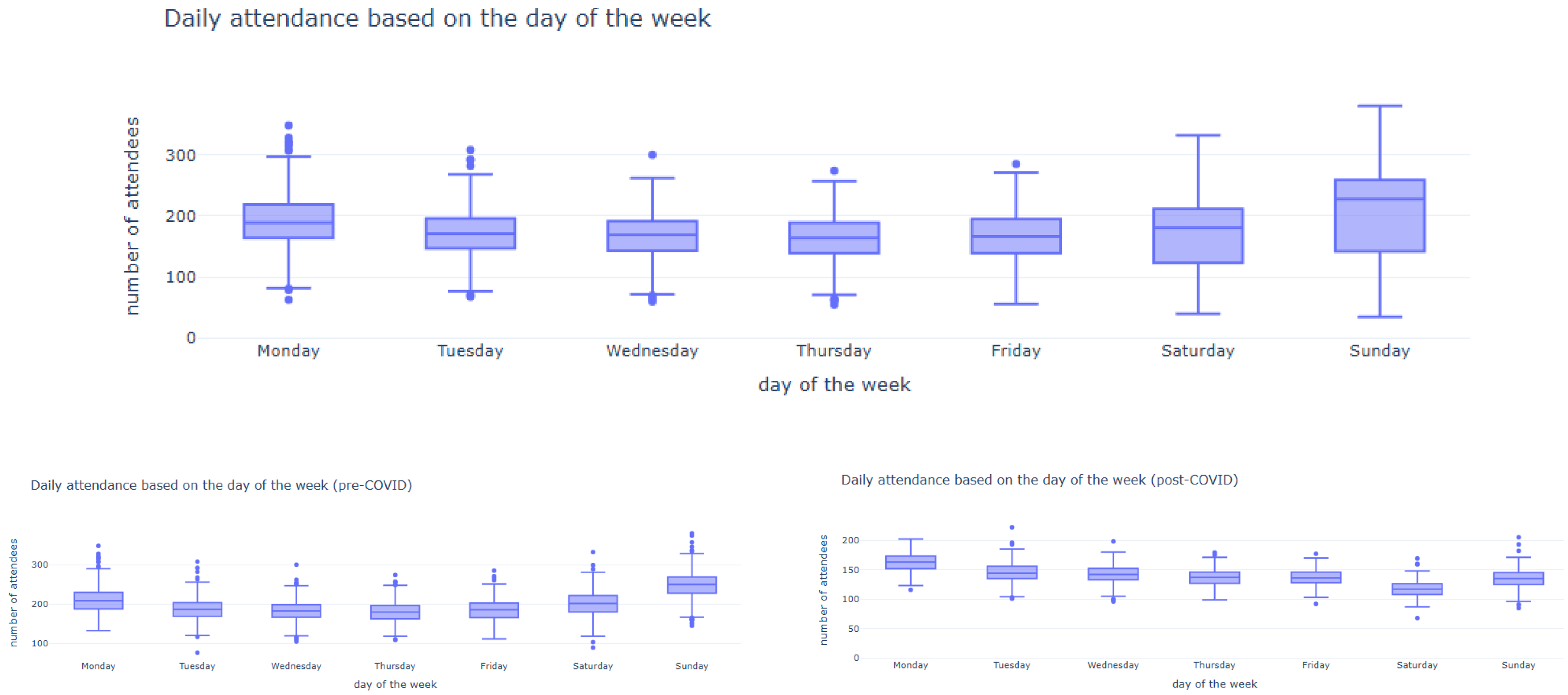
At the weekly level (Figure 5), consistent patterns are also identified. During the precovid period, Sundays recorded the highest number of visits, while Wednesdays had the lowest. In the postcovid period, this pattern changes: Mondays become the day with the highest attendance, and Saturdays the lowest. Furthermore, the variability between days is reduced, which may reflect a reorganization of consultation habits or a redistribution of healthcare workload.

The analysis also considers the influence of public holidays (Figure 6). In both periods, an increase in emergency visits is observed during holidays, although this effect is more pronounced in the precovid period. This may be due to the reduced availability of other healthcare services during holidays, leading to increased use of hospital emergency departments.

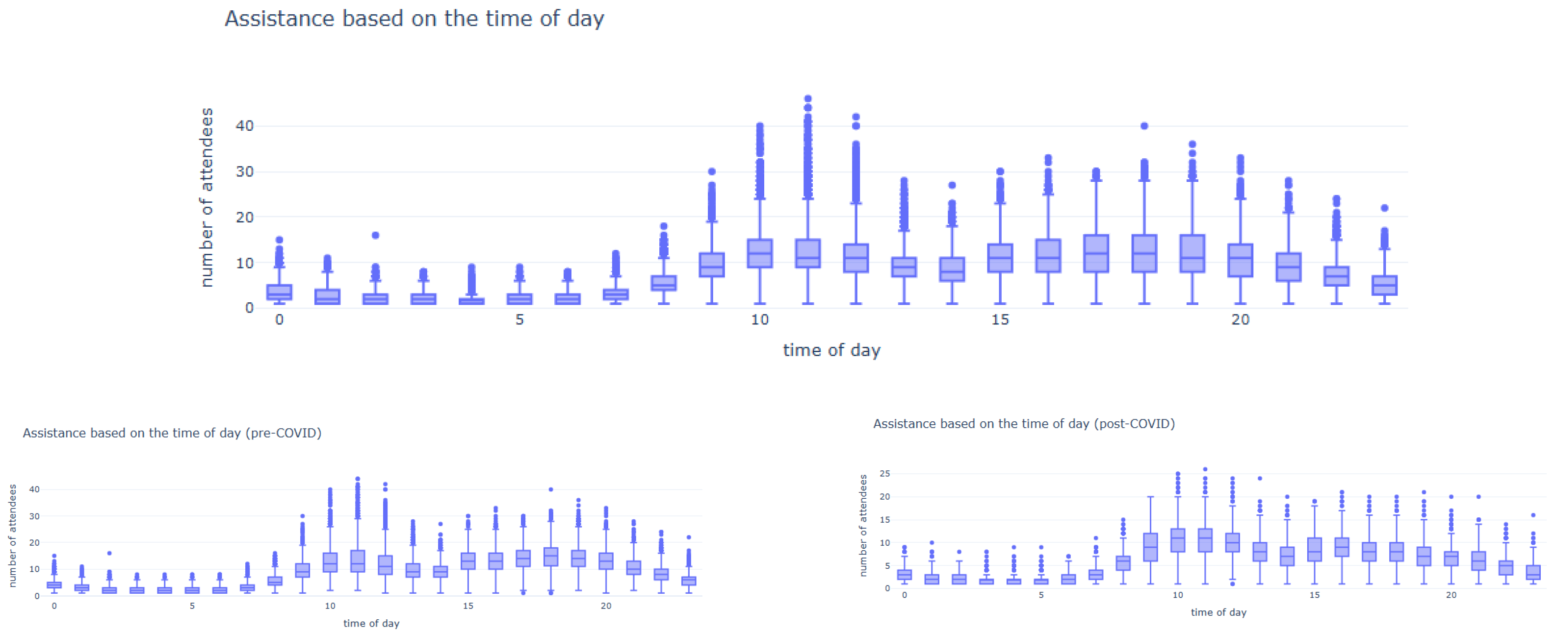
Lastly, the distribution of emergency visits throughout the day is analyzed (Figure 7). Two main peaks are identified: one in the late morning and another in the late afternoon, with a gradual decline during the night. In the precovid period, visit rates were slightly higher in the afternoon, while in the postcovid period, a sharper reduction is observed in both peaks, especially in the afternoon. This decrease is also reflected in the hourly frequency range, which drops from 0–20 in the precovid period to 0–15 in the postcovid period.

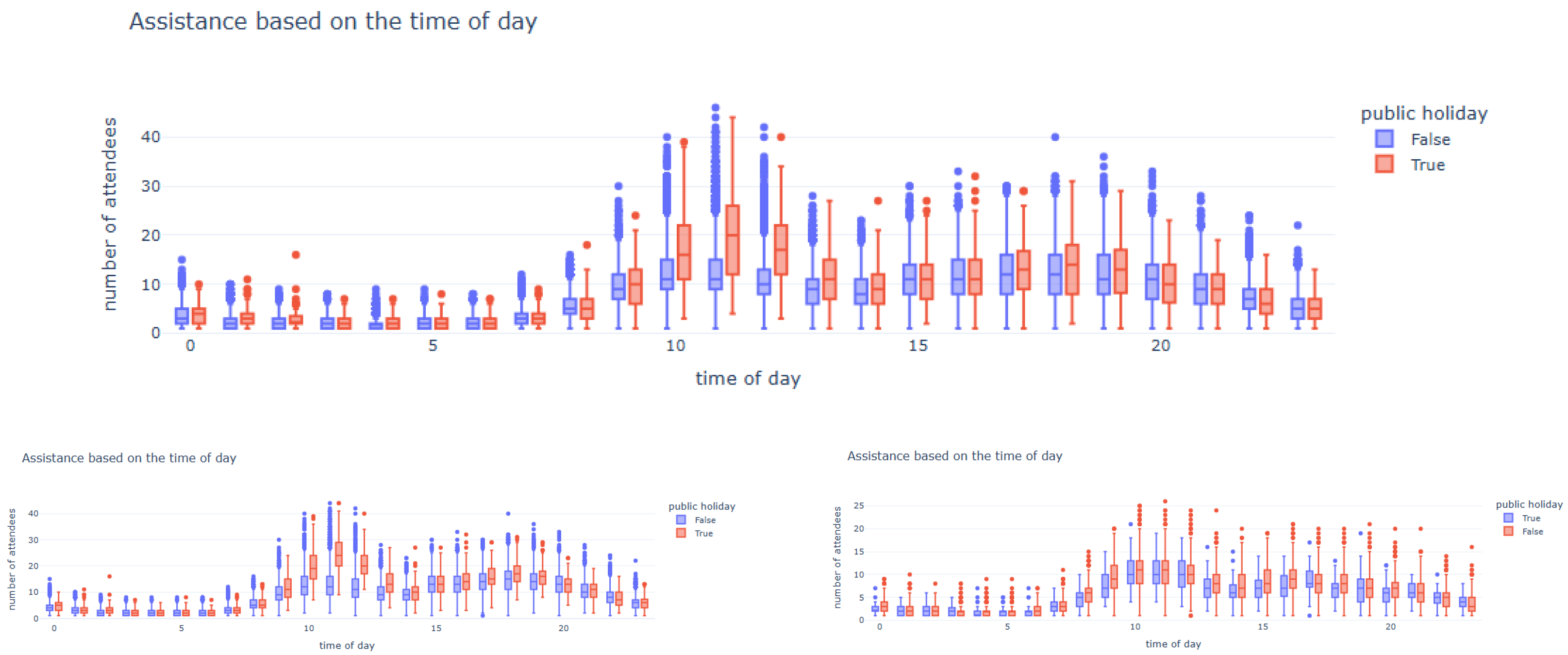
When analyzing hourly emergency visits while distinguishing between public holidays and non-holidays, as shown in Figure 8, it is observed that festive mornings concentrate a higher number of visits, especially during the precovid period. In contrast, this difference nearly disappears in the postcovid period, suggesting a homogenization of healthcare-seeking behavior.

3.2. Descriptive Analysis of the Remaining Variables

After examining the temporal variables, the analysis focuses on the sociodemographic characteristics of patients attending the emergency department, specifically age and gender. These variables help identify the population groups most frequently using emergency services and detect potential structural changes in the patient profile over time.

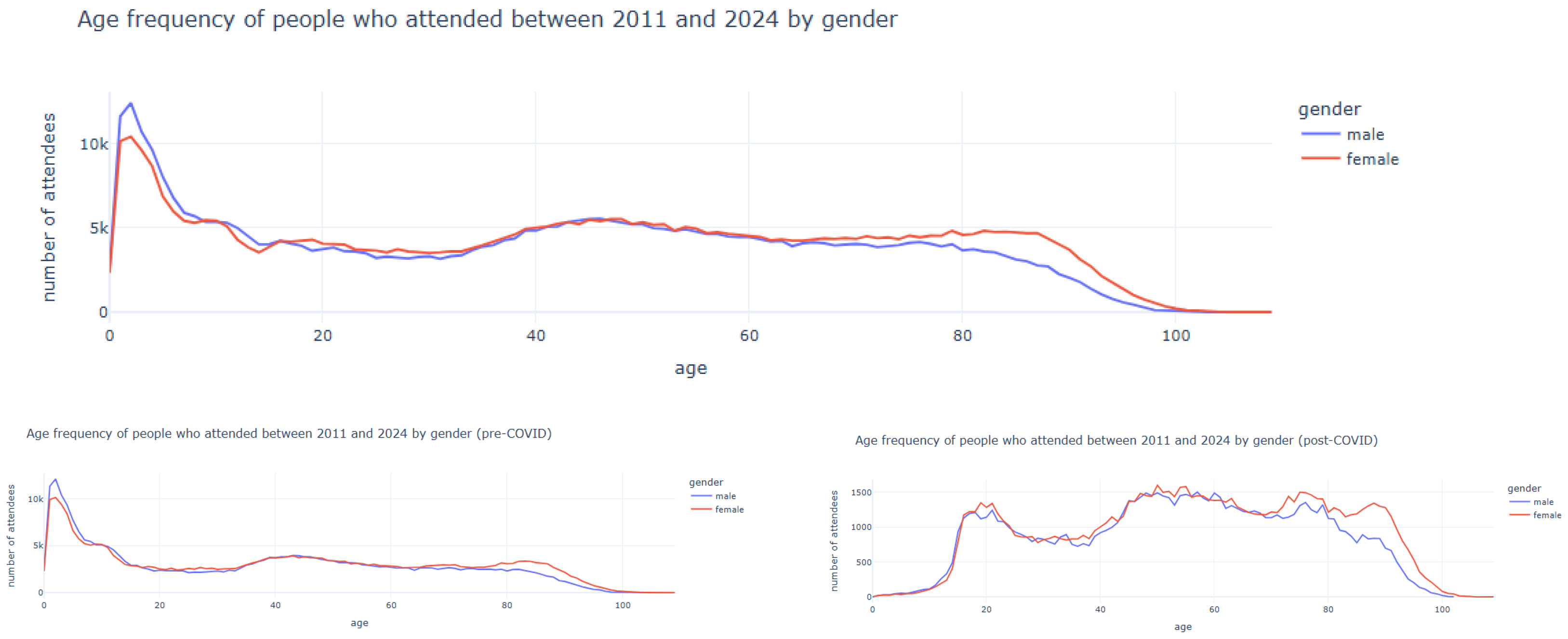
The results are presented in Figure 9. The overall distribution of emergency visits between 2011 and 2024 shows a peak in demand during childhood, particularly in the early years of life (ages 0–8), with a higher proportion of boys than girls. From age 18, the number of visits decreases significantly, reaching its lowest point between ages 18 and 35. From age 40 onwards, demand gradually increases, with women being more represented in older age groups. This reflects both the longer life expectancy of women and their greater presence in the elderly population.

When comparing the precovid period (2011–2019) with the postcovid period (2021–2024), a drastic change in age distribution is observed. In the postcovid period, the pediatric peak in emergency visits disappears, indicating a significant shift in pediatric care. This change is not due to a real decrease in demand, but rather to a reorganization of the healthcare system: during the pandemic, the pediatric emergency unit at Hospital Royo Villanova was closed to repurpose space for COVID-19 patients. Since then, pediatric care has been handled by the Children’s Hospital, the regional referral center, explaining the absence of pediatric patient records in the postcovid data.

This has important implications for the analysis, as it affects comparability between the two periods. While the pediatric population represented a significant portion of demand in the precovid period, in the postcovid era, the patient profile shifts toward older age groups, with a relative increase in adult and elderly patients.

In general, emergency visits are slightly more frequent among women than men, especially from age 40 onward. This difference becomes more pronounced at older ages, where women are not only more numerous in the general population but also exhibit a higher frequency of visits. In contrast, during childhood, boys visit the emergency department more often than girls, although this difference disappears during adolescence.

The third dimension of the analysis focuses on clinical urgency, specifically how each emergency episode is classified, managed, and categorized. This includes variables such as triage level, discharge destination, visit frequency, and main diagnosis, all of which are essential for understanding the nature of the care provided and the clinical profile of patients.

The main diagnosis allows grouping consultation reasons into broad clinical categories. The most frequent categories are

• Injuries and poisoning: prevalent among young and active populations.
• Symptoms, signs, and ill-defined conditions: reflect cases without a clear diagnosis at the time of care.
• Diseases of the respiratory system: very common in winter, though they have declined postcovid.
• Diseases of the musculoskeletal system and connective tissue: frequent among adults.
• Disorders of the nervous system and sense organs: include headaches, vertigo, visual disturbances, etc.

Gender-based analysis reveals differences, such as respiratory diseases being more frequent among men, while endocrine and mental disorders show a more balanced distribution or are slightly more prevalent in women. In the postcovid period, a notable decline in respiratory diseases is observed, possibly related to mask usage, social distancing, and the reorganization of pediatric care.

Triage is the first clinical filter applied to a patient upon arrival at the emergency department. It is classified into five levels:

• Level I: immediate care due to life-threatening conditions.
• Level II: very urgent, with potential risk.
• Level III: urgent but stable.
• Level IV: minor urgency.
• Level V: non-urgent.

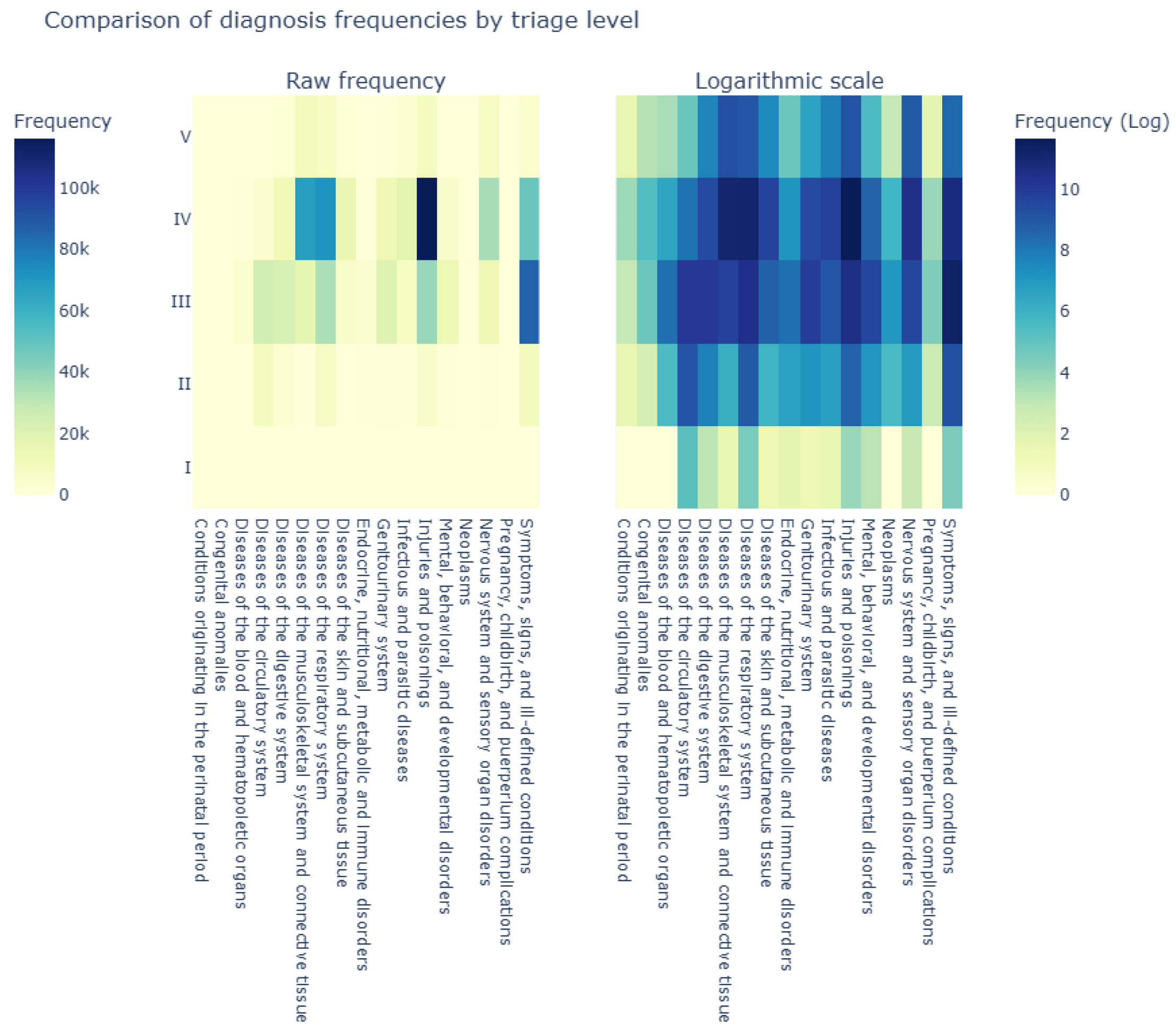
Across the dataset, most patients are classified as Level IV, particularly during the precovid period. However, in the postcovid period, Level III becomes more prominent, which may reflect a change in the types of conditions treated or an increase in the severity of cases arriving at the hospital (Figure 10). When analyzing triage levels by diagnosis, relevant associations are identified (Figure 11):

• Triage Level I shows extremely low frequencies across all diagnostic groups. Only a few cases related to circulatory and respiratory system diseases are identified.
• Triage Level II includes severe conditions such as circulatory and respiratory system diseases, intoxications, or trauma. This clinical profile reflects patients with potential risk requiring priority care.
• Triage Level III represents the greatest diversity and volume of diagnoses. Common diagnoses include nonspecific or ill-defined symptoms, respiratory and digestive diseases, musculoskeletal disorders, and mental and behavioral disorders.
• Triage Level IV shows a notable increase in low-complexity and high-frequency conditions, such as musculoskeletal, respiratory, and dermatological diseases.
• Triage Level V maintains relevant frequencies in respiratory, musculoskeletal, and skin diseases.

Discharge destination indicates how each emergency visit is resolved. The available options include:

• Discharge to home: the most frequent outcome, indicating resolution without the need for hospital admission.
• Hospital admission: the second most frequent, associated with more severe diagnoses.
• Transfer to another facility: such as Hospital Miguel Servet or Hospital Nuestra Señora de Gracia.
• Voluntary discharge, outpatient referral, death, among others.

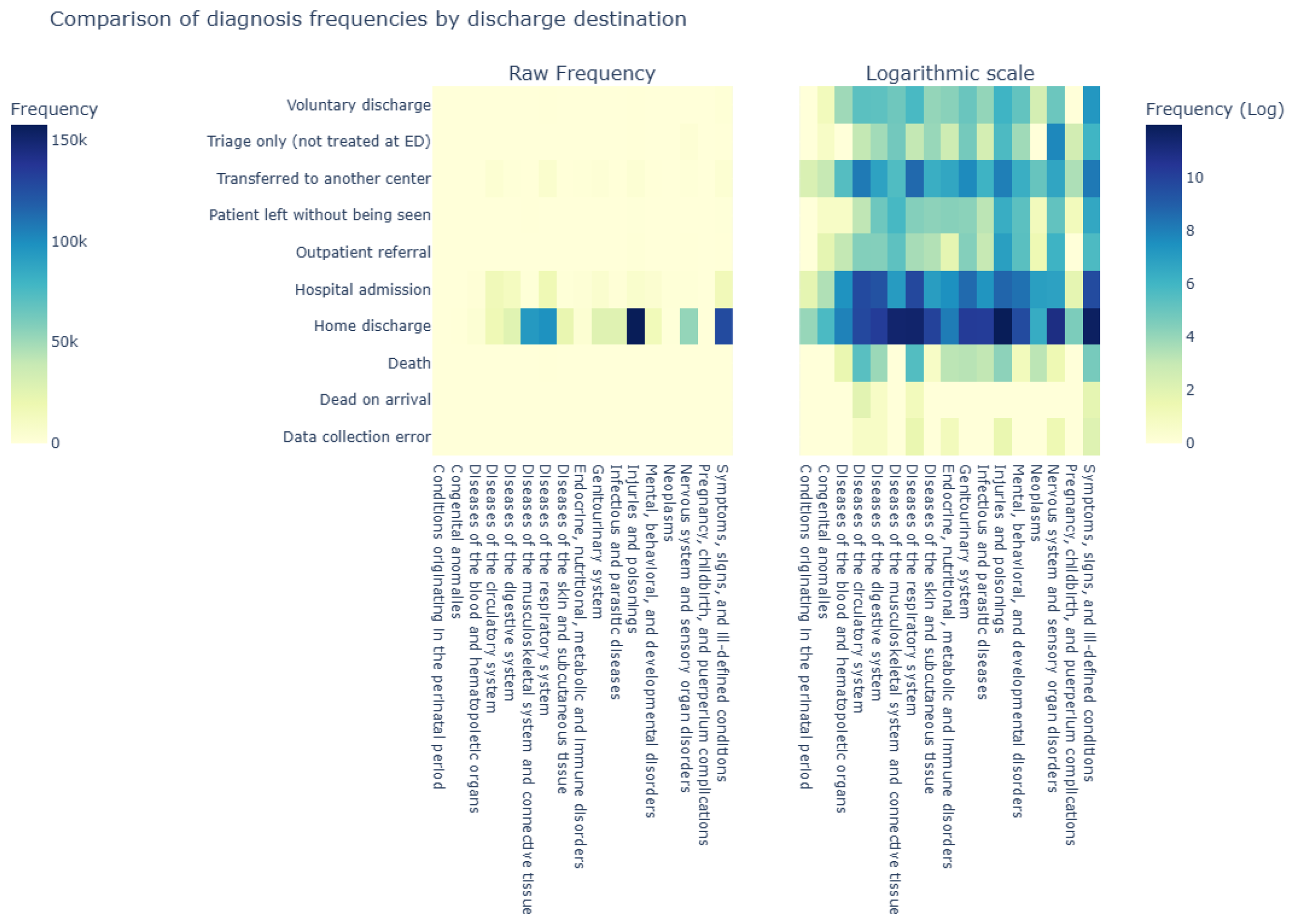
When cross-referencing this variable with the diagnosis (Figure 12), it is observed that neoplasms have a high percentage of hospital admissions (for every two discharges to home, there are three admissions). Circulatory and hematologic diseases also show elevated hospitalization rates, as do digestive system diseases, respiratory system diseases, and mental and behavioral disorders. In contrast, minor injuries, nonspecific symptoms, and less severe conditions are usually resolved with discharge to home.

Deaths and transfers to other centers occur mainly in patients with circulatory and respiratory system diseases, which also correspond to the most frequent diagnoses.

Finally, the frequency of emergency department visits is analyzed, measuring how many times each patient visited the ED during the study period (2011–2024). Results show an average of 4.44 visits per patient who attended at least once, although the median is only 2, indicating that most patients visit infrequently. In the pre-COVID period, the average was 3.84 visits, while in the post-COVID period, the average dropped to 2.15 visits, with a median of 1. This decrease may be related to changes in accessibility, perceived risk, or the reorganization of healthcare services following the pandemic.

3.3. Correlation of Internal Variables

After characterizing the temporal, sociodemographic, and clinical dimensions, the analysis proceeds to examine the correlations among the internal variables of the emergency system. The objective is to identify the factors most strongly associated with visit frequency and to investigate how these associations vary according to the primary diagnosis. The internal variables considered in this study are summarized in

Table 3. Internal variables of the emergency system included in the analysis.

Category	Variable
Demographic	Age
Demographic	Sex
Geographic	Province
Geographic	Basic Health Zone (BHZ)
Clinical	Triage level
Clinical	Discharge destination
Clinical	Destination center
Clinical	Diagnosis
Temporal	Care times (arrival, attention, discharge)
Temporal	Date and time (day, month, year, hour, day of the week)

.

These variables were analyzed both collectively and stratified by diagnosis to uncover diagnosis-specific patterns. Given the heterogeneity in case frequencies across diagnoses,

Table 4. Number of cases per diagnosis category used to contextualize the analysis. Differences in frequencies across diagnoses necessitate this information for proper comparison and interpretation.

Diagnosis	Number of Cases
Congenital anomalies	373
Genitourinary system	35,239
Pregnancy, childbirth, and puerperium complications	146
Endocrine, nutritional, metabolic and immune disorders	5967
Conditions originating in the perinatal period	67
Diseases of the skin and subcutaneous tissue	23,576
Diseases of the blood and hematopoietic organs	4741
Diseases of the digestive system	40,150
Diseases of the respiratory system	121,798
Diseases of the circulatory system	37,371
Diseases of the musculoskeletal system and connective tissue	96,408
Infectious and parasitic diseases	29,051
Injuries and poisonings	169,422
Neoplasms	1806
Nervous system and sensory organ disorders	58,134
Symptoms, signs, and ill-defined conditions	149,026
Mental, behavioral, and developmental disorders	21,099

presents the total number of cases recorded for each diagnosis. This information provides essential context for interpreting the analyses accurately.

An initial analysis examined the variation of these variables across diagnoses. Of the 864,956 records, 8.77% were excluded due to missing diagnosis information. Key demographic, clinical, and temporal variables were selected to describe and compare each diagnostic group (Figure 13), while accounting for substantial differences in case frequencies (Table 4).

Age exhibited notable variation among diagnoses, with median values generally around 44 years; however, circulatory and hematologic diseases showed higher mean ages, approaching 70 years. Certain diagnoses, such as perinatal conditions and infectious diseases, were concentrated in younger age groups, reflecting distinct clinical profiles. Sex distribution was generally balanced across diagnoses, with exceptions including pregnancy-related complications (predominantly female) and neoplasms (slight male predominance).

Spatial analysis at the basic health zone level revealed significant variation for specific diagnoses. Triage level classification identified two distinct groups based on severity and urgency, particularly for circulatory and hematologic diseases. Discharge destination also correlated with diagnosis, with higher hospital admission rates observed for neoplasms and other systemic conditions.

Temporal patterns exhibited consistent peaks during morning and evening hours, with additional weekly and seasonal fluctuations. Notably, respiratory and infectious diseases displayed decreased incidence during summer months. Analysis of waiting times revealed considerable variability, with certain diagnoses associated with substantially longer average stays, reflecting the complexity and resource demands of urgent care.

Since many of the internal variables are categorical or exhibit non-normal distributions, the Spearman correlation coefficient was employed to assess monotonic relationships without assuming linearity or normality. This approach is particularly appropriate for cyclical temporal variables, such as time of day and day of the week.

The results indicate that time of day is the temporal variable most strongly associated with attendance frequency, with particularly pronounced correlations for diagnoses such as those reported in

Table 5. Correlation of time of day with attendance frequency by diagnosis.

Diagnosis	$\mathit{\rho }$
Injuries and poisonings	0.49
Respiratory diseases	0.32

.

Other temporal variables, including day of the week, month, and year, exhibited low or negligible correlations for most diagnoses, indicating limited or indirect influence. A slight positive correlation with day of the week was observed for infectious and parasitic diseases, as well as mental disorders, particularly during weekends. Conversely, correlation with year was generally negative, suggesting a declining trend in attendance frequency for certain diagnoses, as summarized in

Table 6. Negative correlation of year with attendance frequency.

Diagnosis	$\mathit{\rho }$
Respiratory diseases	−0.20
Infectious diseases	−0.13

.

When considering all diagnoses collectively, time of day remains the most influential temporal variable, whereas the impact of other temporal variables is comparatively minor (

Table 7. Correlation of temporal variables with attendance frequency across all diagnoses.

Variable	$\mathit{\rho }$
Time of day	0.56
Day of the week	0.01
Month	−0.01
Year	−0.14

).

These findings reinforce that hourly variation constitutes the most stable and predictable pattern in healthcare demand, whereas other temporal variables exhibit more diffuse or context-dependent effects.

Following the identification of preliminary correlations between internal variables and emergency department visits, a model-based approach was undertaken to determine the variables most relevant for predicting patient demand. The XGBoost algorithm was employed, enabling the assessment of feature importance using the three metrics defined in Section 2.3.

Feature importance values were computed using the get_score() method from the xgboost Python (version 3.0.5) library running on Python 3.13.7, specifying the importance_type parameter as "gain", "cover", and "weight", respectively. Each metric is derived from the internal structure of the trained gradient boosting trees and reflects the extent to which the model relies on each feature during training.

The results, presented in

Table 8. Internal variable importance metrics. Hour stands out in all metrics.

Diagnosis	Gain				Cover				Weight
	Month	Year	Hour	Day	Month	Year	Hour	Day	Month	Year	Hour	Day
Congenital anomalies	0.37	0.48	0.86	0.33	274	1401	3289	408	333	305	309	225
Genitourinary system	1.01	2.05	42.40	0.98	2568	5844	17,179	2993	1835	1532	924	1696
Pregnancy, childbirth and puerperium complications	0.37	0.47	0.52	0.48	138	838	1343	173	65	99	108	52
Endocrine, nutritional, metabolic and immunity disorders	0.56	0.66	9.46	0.56	1474	2045	7293	1788	1338	1416	823	1178
Perinatal conditions	0.40	0.35	0.39	0.44	72	243	822	29	42	42	72	25
Diseases of the skin and subcutaneous tissue	1.09	5.00	21.86	1.88	2473	3957	9071	3658	1732	1534	1228	1416
Diseases of blood and blood-forming organs	0.55	0.58	14.62	3.78	1097	1293	6669	3125	985	1083	855	766
Diseases of the digestive system	0.99	2.68	29.29	1.28	3039	5784	14,932	4199	1810	1565	1115	1609
Diseases of the respiratory system	39.54	69.36	143.61	31.59	11,786	15,710	25,064	8783	1907	1553	1372	1401
Diseases of the circulatory system	1.11	1.28	48.57	2.53	3505	4008	16,425	4097	1925	1718	1005	1461
Diseases of the musculoskeletal system and connective tissue	2.56	9.33	159.80	2.93	5745	11,763	34,693	6539	1899	1496	1071	1627
Infectious and parasitic diseases	2.95	13.52	33.65	6.22	3129	4568	9717	3599	1856	1570	1270	1409
Injuries and poisoning	5.50	23.76	253.92	6.80	11,922	18,359	50,815	12,192	2026	1513	1131	1507
Neoplasms	0.47	0.47	3.65	0.72	606	771	5020	2365	813	784	661	604
Nervous system and sense organs	2.61	18.68	88.92	8.49	3808	8165	18,999	5187	1892	1630	1156	1469
Symptoms, signs and ill-defined conditions	2.61	9.34	116.57	3.21	10,674	16,728	44,466	10,511	1929	1667	1092	1529
Mental, behavioral and developmental disorders	0.88	1.63	19.52	1.35	1958	4851	9623	3016	1776	1463	1069	1402
Total	12.78	92.40	856.08	27.94	572,702	118,146	320,698	96,716	2032	1619	1162	1404

, indicate that the hour of the day is consistently the most important variable across all diagnoses and metrics. Secondary contributions were observed for:

• Year, reflecting long-term trends.
• Day of the week, capturing weekly attendance patterns.
• Month, with lower weight but relevance for diagnoses exhibiting clear seasonality, such as respiratory diseases.

This pattern holds in both the overall analysis and most individual diagnoses. For instance, in injuries and poisonings, the hour of the day exhibits the highest importance, indicating strong temporal clustering. For respiratory diseases, both month and year gain relevance, reflecting seasonal variation and post-pandemic trends. In mental disorders, the day of the week becomes more influential, with higher attendance observed at the beginning of the week.

For predictive evaluation, gain was selected as the reference metric for variable importance, as it represents the average contribution of each feature to reducing the model’s loss, providing a more accurate measure of predictive relevance compared to cover or weight.

Model performance was assessed (

Table 9. Performance metrics for the global model using an increasing number of variables (ordered by gain).

Variables	MAE	RMSE	${\mathit{R}}^{\mathbf{2}}$	${\mathbf{ACC}}_{\mathbf{3}}$ (%)
1	2.72	14.51	0.51	72.41
2	2.43	11.61	0.61	77.33
3	2.21	9.49	0.68	80.08
4	2.10	8.31	0.72	81.64

and

Table 10. Performance metrics for respiratory diseases using an increasing number of variables (ordered by gain).

Variables	MAE	RMSE	${\mathit{R}}^{\mathbf{2}}$	${\mathbf{ACC}}_{\mathbf{3}}$ (%)
1	1.03	2.48	0.15	96.72
2	0.95	2.17	0.26	97.04
3	0.85	1.79	0.39	97.59
4	0.77	1.39	0.52	98.26

) using standard metrics: Mean Absolute Error (MAE), Root Mean Squared Error (RMSE), and $R^2$. Additionally, ${\mathrm{ACC}}_n$ was reported, representing the proportion of predictions within $\pm n$ patients of the observed value. This metric is particularly relevant for operational planning, as it reflects the practical accuracy of the model in forecasting hourly emergency department attendance.

Models for rare diagnoses exhibited lower predictive performance, likely due to limited sample sizes, whereas common diagnoses, such as respiratory diseases, achieved substantially better results, with MAE below 1 and ${\mathrm{ACC}}_3$ exceeding 98%.

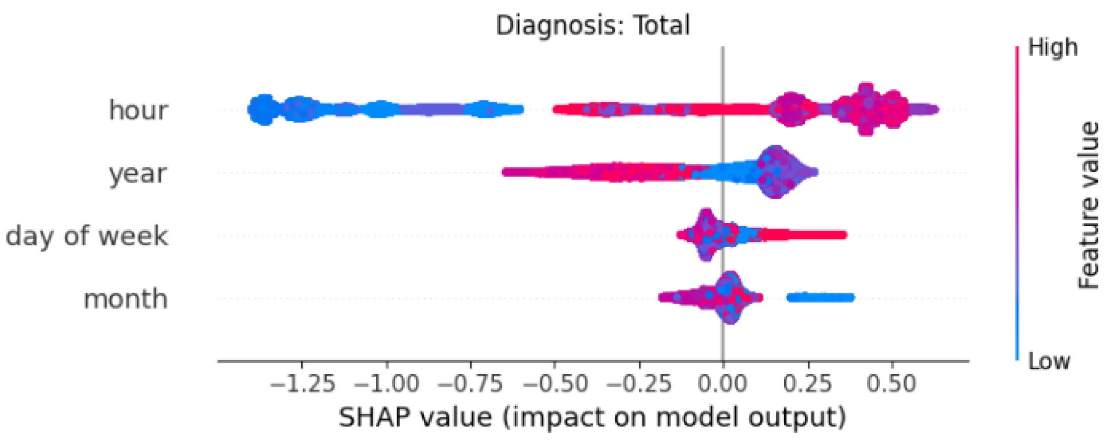
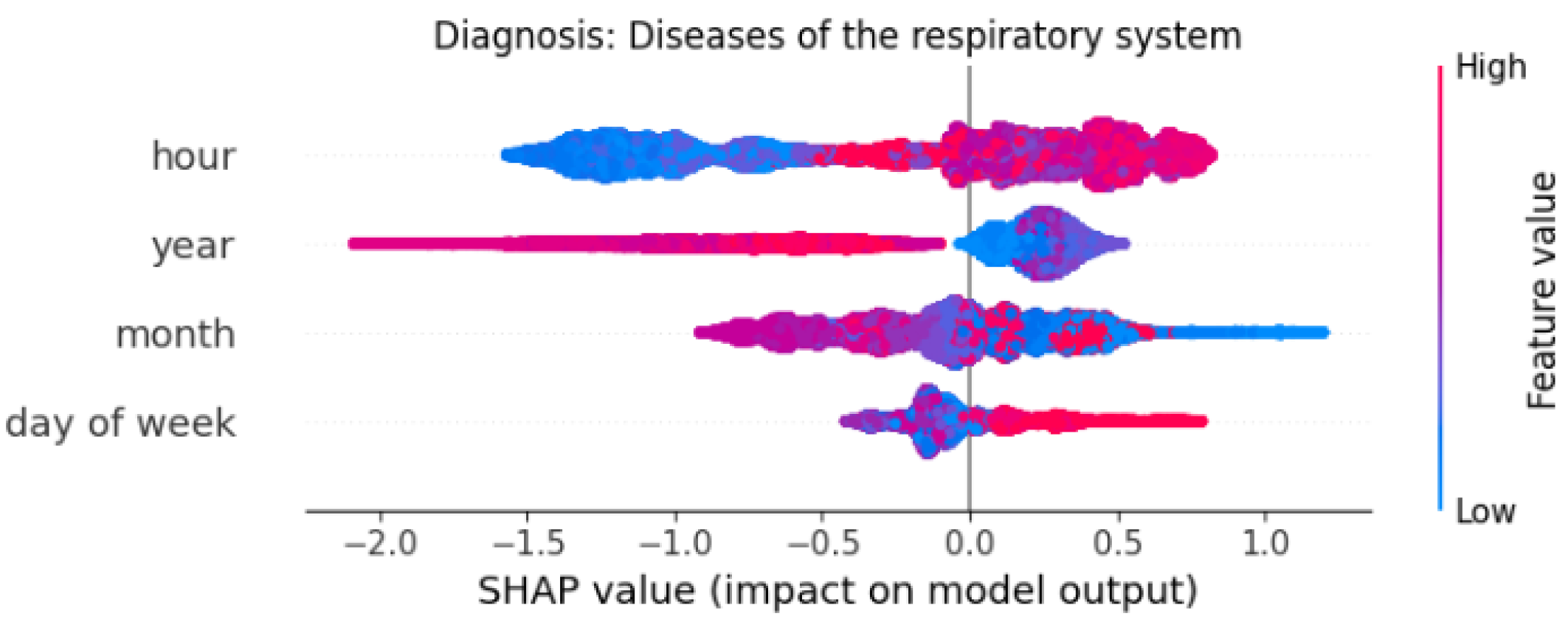
To further interpret the influence of individual variables on attendance, SHAP (SHapley Additive exPlanations) plots were utilized to visualize the effect of each feature value on model predictions. Key observations include

• Hour of the day: Early morning hours are associated with lower predicted attendance, whereas mid-morning and afternoon periods increase the likelihood of visits (Figure 14).
• Day of the week: Weekend days tend to increase attendance, particularly for diagnoses such as infectious or respiratory diseases.
• Month: Winter months are associated with higher attendance in respiratory diseases (Figure 15), while no clear seasonal pattern is observed for other diagnoses.
• Year: Certain diagnoses, particularly pediatric and respiratory conditions, exhibit a progressive decrease in attendance following 2020 (Figure 16).

3.4. Seasonality and Temporal Autocorrelation

Following the identification of the most relevant internal variables, the analysis focused on examining whether the data exhibit repetitive patterns (seasonality) and whether their statistical properties remain stable over time (stationarity).

Seasonality refers to periodic fluctuations that recur at regular intervals, such as weekly, monthly, or yearly cycles. To detect such patterns, autocorrelation plots (ACF) were generated at multiple temporal scales (Figure 17 and Figure 18):

• Daily: Strong autocorrelation is observed between consecutive days, particularly for respiratory diseases, where values remain elevated for several days consecutively.
• Weekly: Clear cyclical patterns are detected, with attendance peaks on specific days of the week (e.g., Mondays or Sundays, depending on the diagnosis).
• Monthly: For certain diagnoses, such as respiratory diseases, a pronounced peak in autocorrelation occurs in month 12, indicating strong annual seasonality.
• Every 4 h and every 15 days: These finer temporal scales exhibit less consistent patterns; however, some diagnoses show repeated behaviors in specific intervals.

These results indicate that seasonality is pronounced at daily and weekly levels and particularly evident on an annual scale for seasonally affected diagnoses, such as respiratory diseases.

To evaluate stationarity, the augmented Dickey–Fuller (ADF) test was applied. This test assesses the presence of a unit root, which would indicate non-stationarity. In all analyzed series, the ADF test yielded p-values close to zero, allowing rejection of the null hypothesis and supporting the conclusion that the series are stationary.

In practical terms, this implies that despite the presence of seasonal fluctuations, the statistical properties of the time series (mean, variance, and autocorrelation) remain stable over time, providing favorable conditions for subsequent modeling efforts.

3.5. External Variables

The analysis of emergency department demand cannot be separated from the environment in which it occurs. Accordingly, a set of external variables potentially influencing observed variability, either directly or indirectly, was incorporated. These variables were classified according to their temporal frequency into four main blocks: hourly, daily, monthly, and yearly. Their integration facilitates the identification of patterns not solely attributable to internal healthcare system factors.

3.5.1. Hourly External Variables

Hourly variables include environmental and meteorological data with high temporal resolution, obtained from monitoring stations proximal to Hospital Royo Villanova. The variables considered are

• Air pollutants: nitrogen dioxide (NO₂), nitrogen oxides (NO_x), carbon monoxide (CO), tropospheric ozone (O₃), and particulate matter (PM10).
• Weather conditions: air temperature and relative humidity.

Overall correlations between these variables and hourly attendance are low, reflecting the influence of multiple concurrent factors. Nevertheless, relevant associations emerge for specific diagnoses:

• Respiratory diseases: show a positive correlation with NO₂ ($\rho \approx 0.18$), suggesting a possible adverse effect of urban pollution. A negative correlation with O₃ is also observed, consistent with previous studies on oxidant toxicity.
• Injuries and poisonings: exhibit a positive correlation with O₃ ($\rho \approx 0.25$), possibly related to increased outdoor activity on sunny days, with greater ozone exposure.
• Musculoskeletal system diseases: slight correlations are detected with NO and O₃, although with less consistency across years.

3.5.2. Daily External Variables

At the daily scale, meteorological coverage is expanded and additional pollutants are incorporated:

• Weather: accumulated precipitation, wind speed, atmospheric pressure, and sunshine hours.
• Additional pollutants: benzene (C₆H₆) and sulfur dioxide (SO₂).

At this temporal resolution, associations with attendance are more apparent:

• Respiratory diseases: negative correlation with daily average temperature ($\rho \approx -0.43$), sunshine hours, and pressure, and positive correlation with relative humidity and C₆H₆, suggesting that cold and humid conditions, along with pollution, increase demand.
• Injuries and poisonings: positively associated with warm and sunny days, where exposure to external risks is likely higher.
• Mental disorders: show a marked weekly distribution, with peaks at the beginning of the week, pointing to organizational or social components of healthcare-seeking behavior.

3.5.3. Monthly External Variables

Monthly variables incorporate aggregated economic and social indicators that reflect macroeconomic context and population mobility:

• Economy: unemployment rate, number of signed contracts (total and temporary).
• Mobility: number of national and international tourists in the province.

Observed patterns include

• Digestive and skin diseases: positive correlation with unemployment and negative with job creation, which may reflect greater social vulnerability.
• Respiratory diseases: negative correlation with temperature and tourism, and positive with pollution levels, suggesting a combined effect of adverse weather and air pollution.
• Mental disorders: show a slight positive correlation with tourism, possibly related to stress caused by urban crowding or disruptions in daily routines.

3.5.4. Annual External Variables

At the annual scale, structural variables characterize sociodemographic composition and territorial inequality:

• Average age, dependency rate (<16 and >65 years), average annual income, Gini index, average household size, and single-parent household rate.

Despite the limited number of observations (14 years), consistent relationships were observed:

• Child dependency rate: strong positive correlation with attendance in several diagnostic categories.
• Average income and population over 65 years: negative correlation with total demand, which may reflect better access to preventive care or lower exposure to risk factors.
• Gini index and average household size: positive correlations, consistent with studies linking inequality to higher use of emergency services.

3.5.5. Integration into the Explanatory Analysis

Although predictive modeling was not the primary objective, an XGBoost model with a Poisson distribution was applied as an explanatory tool. SHAP values were used to quantify the local contribution of each variable. Key findings by temporal frequency include

• Hourly frequency: Temperature and relative humidity stand out as the most influential variables globally. Although pollutants are less relevant in global terms, they show significant local impacts in diagnoses such as respiratory or musculoskeletal diseases.
• Daily frequency: Variables such as CO and PM10 appear as important across multiple diagnostic groups. Daily mean temperature acts as a discriminator between diagnoses: cold days increase respiratory diseases, while warm days elevate injury cases.
• Monthly frequency: Unemployment and tourism modulate demand in digestive, dermatological, and psychiatric diagnoses. Temporary contracts also have a marginal effect.
• Annual frequency: The child dependency rate and the Gini index show considerable explanatory weight, highlighting the importance of structural sociodemographic context.

3.5.6. Diagnosis-Level Evaluation

The influence of external variables varies across diagnoses:

• Respiratory diseases: the inclusion of temperature, SO₂, and NO significantly improves explanatory accuracy, reaching up to 98% accuracy within narrow error margins ($\pm 3$ patients).
• Injuries and poisonings: temperature and seasonality (month) explain a large part of the observed variability.
• Mental disorders: day of the week and temperature emerge as key factors in attendance patterns.
• Neoplasms and congenital anomalies: show low sensitivity to external variables, suggesting a more stable demand or less dependence on the immediate environment.

It is important to emphasize that detected associations do not imply causality. Observed correlations may be mediated by unobserved factors, such as individual characteristics, healthcare organization, or structural changes not captured by the included variables. Additionally, the aggregated nature of some data sources (particularly monthly and annual) limits robust inference regarding directional effects.

Consequently, these results should be interpreted as exploratory evidence for hypothesis generation regarding environmental influences on healthcare demand. Establishing robust causal relationships would require additional strategies, such as structural models, counterfactual analyses, or quasi-experimental designs tailored for time series or panel data.

3.6. Diagnosis-Specific Analysis

After characterizing both internal and external variables, a detailed analysis was conducted at the level of clinical diagnosis, aiming to identify specific patterns of healthcare demand according to pathology type. This approach facilitates the tailoring of management and predictive strategies to the particularities of each diagnostic group.

Statistical methods were employed to assess whether observed differences between diagnoses were quantitatively significant. To this end, the Kruskal–Wallis test was applied to evaluate whether emergency department attendance varies significantly across diagnostic categories. This non-parametric method was chosen over ANOVA due to violations of normality and homoscedasticity in the data, particularly for diagnosis and day-of-week variables. The Kruskal–Wallis test is appropriate for comparing multiple independent groups without these assumptions.

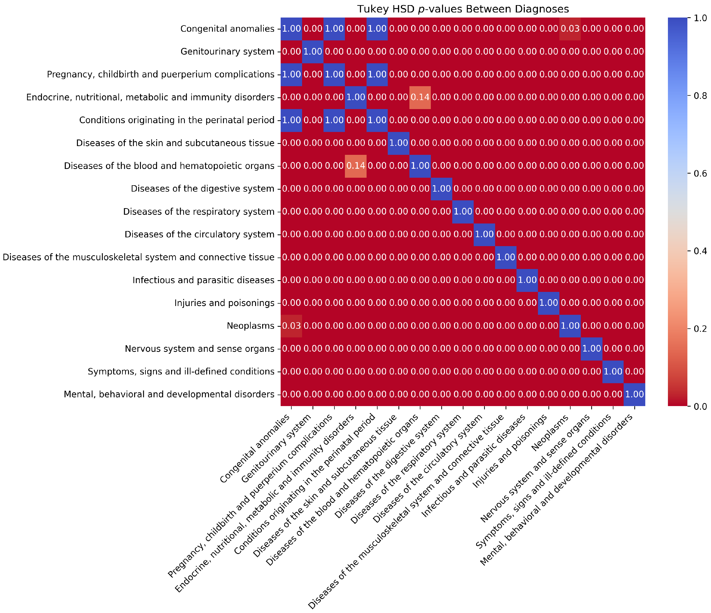
The null hypothesis stated that attendance is independent of diagnosis. The resulting p-value was 0, indicating statistically significant differences in attendance across diagnostic categories. Tukey’s post-hoc test was subsequently applied to identify specific pairs of diagnoses with distinct behaviors. The results of this pairwise comparison are illustrated in Figure 19, where lower p-values indicate the most divergent diagnostic groups.

This analysis confirmed that healthcare demand is heterogeneous across diagnoses, with each group exhibiting unique patterns in terms of

• Temporal distribution: some diagnoses, such as respiratory diseases, show strong seasonality; others, such as injuries, are more tied to time of day or day of the week.
• Triage level: this varies significantly, with circulatory and hematologic diseases concentrated in high acuity levels (I–III), while musculoskeletal or nervous system disorders are predominant in lower levels (IV–V).
• Discharge outcome: this also differs, diagnoses like neoplasms or circulatory diseases show higher admission rates, while others are mostly resolved with discharge home.
• Mean patient age: varies widely across diagnoses, from pediatric conditions (infectious, respiratory) to chronic diseases in older adults (circulatory, neoplasms).

This diagnosis-specific approach not only statistically validates differences between diagnostic groups but also enables precise characterization of each group’s care profile. Such insights are essential for developing targeted predictive models and designing management strategies tailored to the unique demands of each diagnosis.

3.7. Spatial Analysis

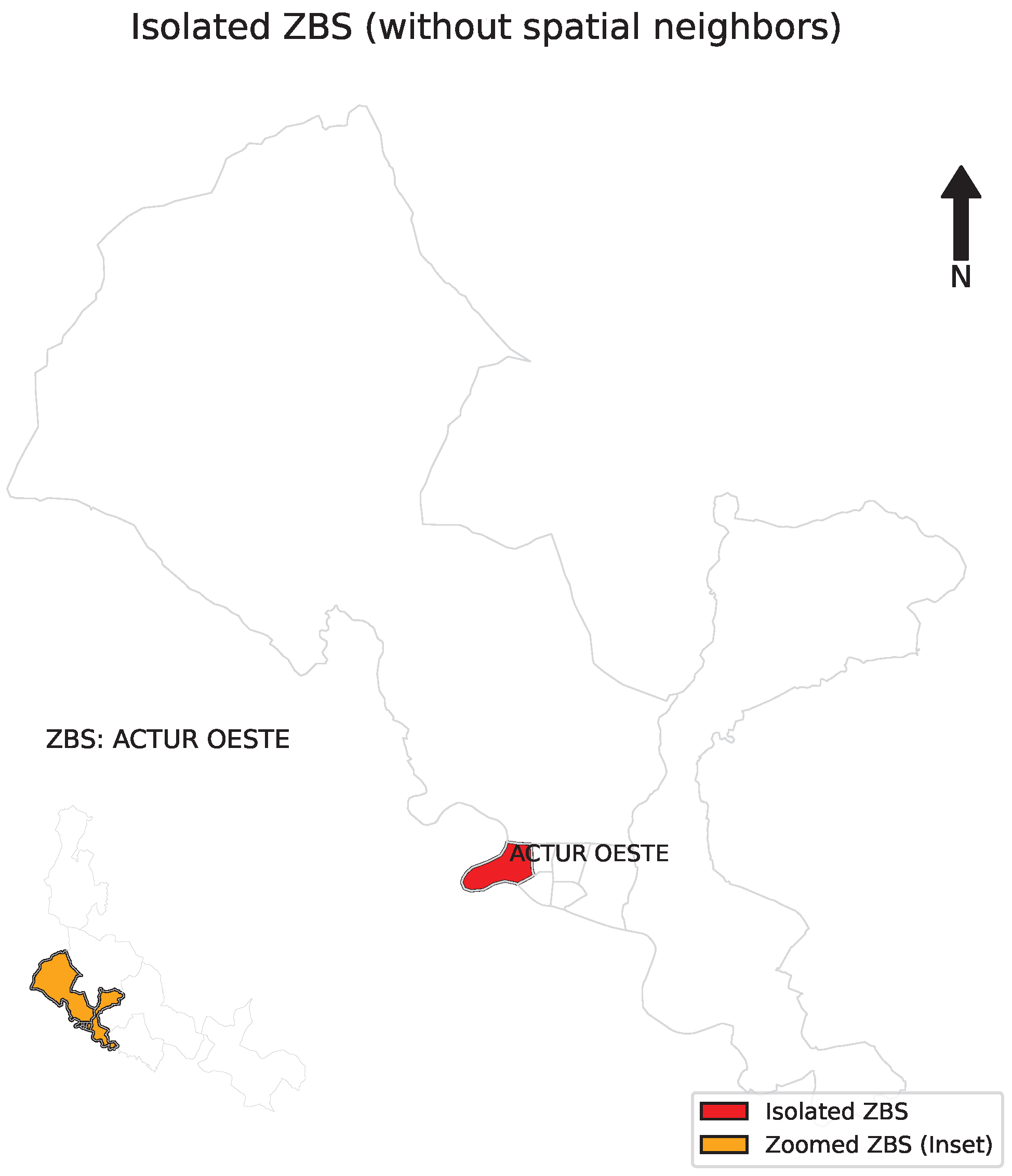
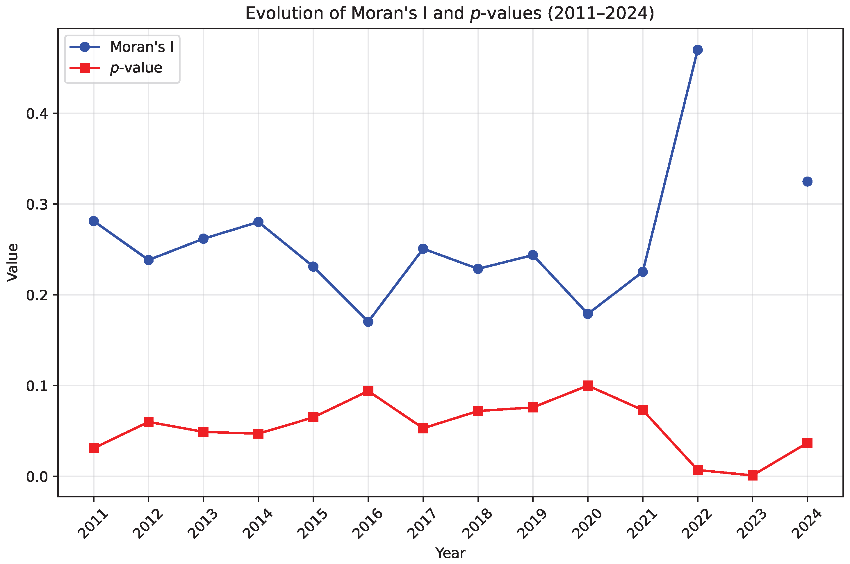
The global Moran’s I index was computed for each year to assess the spatial autocorrelation of attendance rates across Basic Health Zones (BHZs). The spatial weight matrix was defined using first-order Queen contiguity. The topology revealed one BHZ without spatial neighbors (Figure 20), which may affect the estimation of Moran’s I and the detection of spatial patterns, as the calculation relies on spatial contiguity between territorial units. To verify whether this isolated unit influenced the spatial results, Moran’s I was recalculated excluding it. The index remained positive and statistically significant (I = 0.388, p = 0.028 with all units; I = 0.319, p = 0.044 excluding the isolated BHZ), indicating that the global spatial clustering is robust to the inclusion of the isolated area.

Moran’s I quantifies the degree of spatial autocorrelation in georeferenced data, ranging from $-1$ to $+1$ (Figure 21). Positive values indicate spatial clustering, values near zero suggest a random spatial distribution, and negative values reflect spatial dispersion among neighboring areas. Statistical significance is assessed via a p-value, indicating whether the observed pattern differs from random expectation.

Moran’s I values range from a minimum of 0.170 (2016) to a maximum of 0.470 (2022). Using a significance level of 0.05, three temporal periods are identifiable:

• 2011–2014: Consistent significant spatial clustering, with Moran’s I $\ge 0.23$ and p < 0.05.
• 2015–2021: Decline in Moran’s I and p-values above 0.05, indicating weakening or loss of spatial clustering.
• 2022–2024: Strong clustering observed, peaking at Moran’s I = 0.470 in 2022 (p = 0.005). Although reduced in 2024, clustering remains statistically significant.

These results reveal temporal dynamics in the spatial distribution of attendance, potentially reflecting changes in social, demographic, or healthcare system factors.

LISA Analysis

Local Indicators of Spatial Association (LISA) detect spatial autocorrelation at the local level, identifying clusters of high or low values and outlier zones. This complements the global Moran’s I index by revealing spatial heterogeneity.

LISA categories include

• High–High (HH): Zones with high values surrounded by high-value neighbors.
• Low–Low (LL): Zones with low values surrounded by low-value neighbors.
• High–Low (HL): Zones with high values surrounded by low-value neighbors (potential outliers).
• Low–High (LH): Zones with low values surrounded by high-value neighbors (potential outliers).

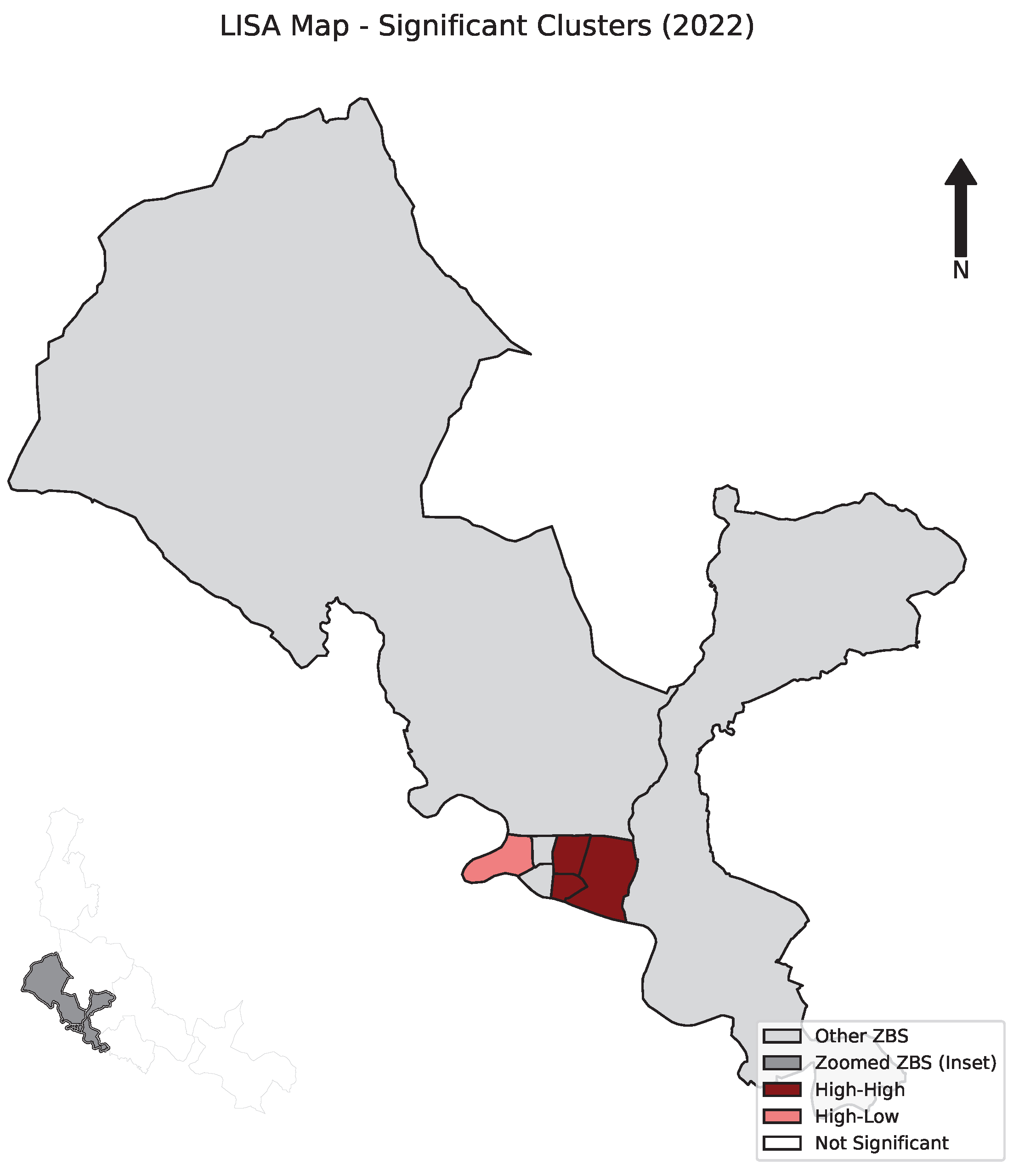
The 2022 LISA analysis (Figure 22) identifies local clusters corresponding to the year with the highest global Moran’s I. Out of 13 zones, 4 exhibit significant spatial association ($p<0.05$):

• High–High (HH): Zalfonada, Arrabal, and Avenida Cataluña, forming a contiguous cluster of high attendance.
• High–Low (HL): Actur Oeste, exhibiting high attendance but surrounded by zones with low attendance, consistent with its spatial isolation.

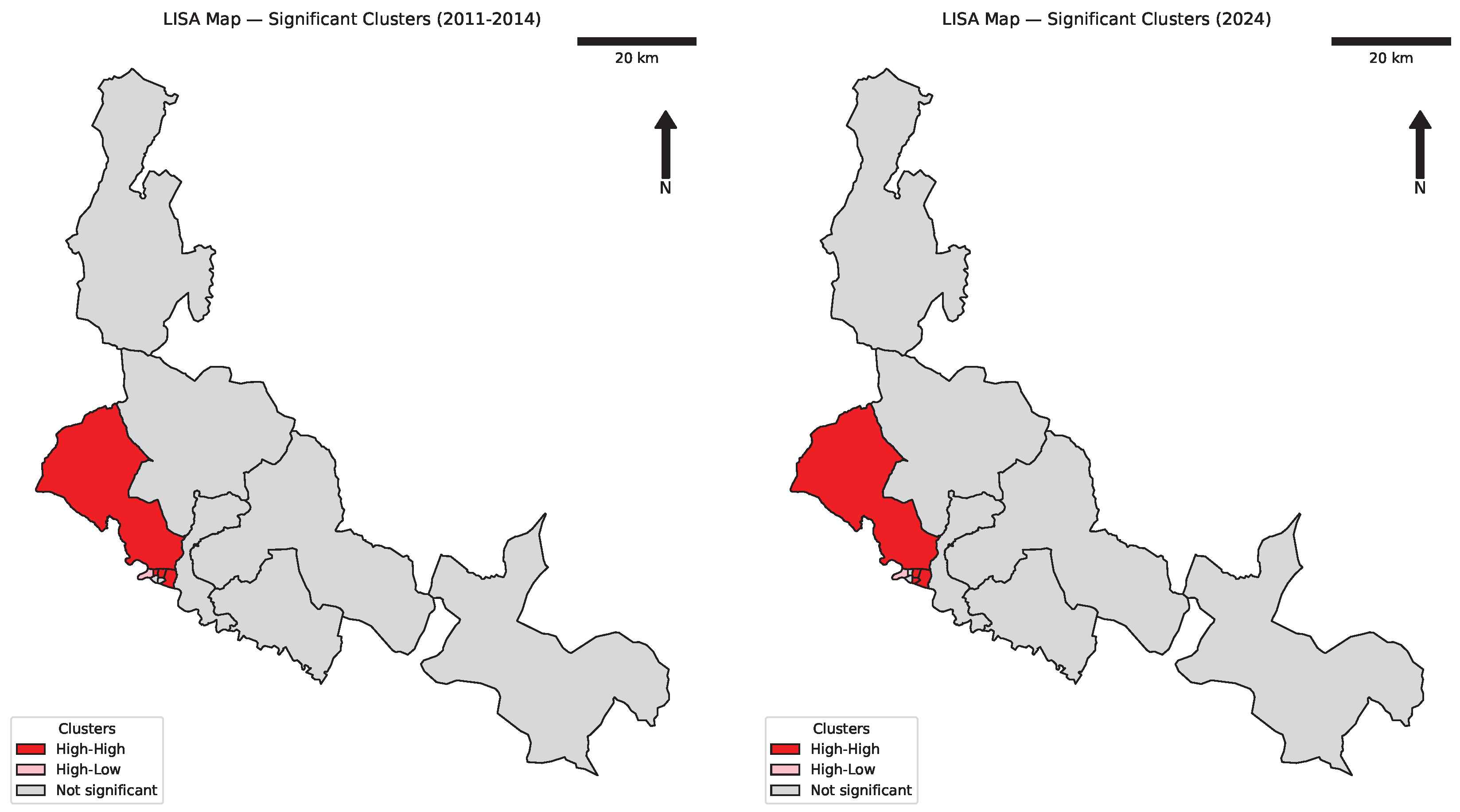
Further LISA analysis for years with significant global Moran’s I (2011–2014 and 2024) reveals stable spatial patterns. During 2011–2014, a persistent HH cluster is observed including Zalfonada, Actur Norte, Parque Goya, and Avenida Cataluña, indicating a consolidated hotspot of high demand (Figure 23).

In 2024, the pattern resembles that of 2022, with Parque Goya joining the HH cluster and Zalfonada no longer included, suggesting minor reconfiguration of the spatial hotspot while maintaining the general geographic concentration of high-demand zones.

4. Discussion

This study presents a novel methodological framework that integrates geospatial analysis with machine learning techniques to investigate emergency department (ED) demand. Unlike traditional approaches based on linear regression or time series models, this framework allows for simultaneous modeling of nonlinear relationships, spatial dependencies, and temporal fluctuations. The use of interpretable machine learning (XGBoost combined with SHAP) enhances both predictive accuracy and explanatory capacity, enabling the identification of localized patterns and variable importance across diagnostic categories. This hybrid approach represents a methodological advancement in health geography and demand forecasting, offering a scalable and generalizable model for urban healthcare systems [20].

The findings corroborate prior research emphasizing the influence of environmental, demographic, and socioeconomic factors on ED utilization [5,9,12]. Specifically, the observed associations between air pollutants (e.g., ${\mathrm{NO}}_2$, ${\mathrm{SO}}_2$) and respiratory conditions reinforce established evidence regarding the health impacts of urban air quality [10]. Moreover, the detection of consistent hourly and seasonal patterns underscores the relevance of temporal dynamics for operational healthcare planning [6].

From a practical perspective, these results have direct implications for hospital resource management. The strong predictive power of the hour of the day variable suggests that staffing and equipment allocation can be dynamically adjusted according to specific time slots. Additionally, the identification of persistent spatial clusters through Moran’s I and LISA analyses provides actionable insights for targeted interventions in high-demand zones, supporting territorial equity in service provision.

Beyond temporal and environmental influences, accessibility to healthcare facilities is a well established determinant of service utilization patterns. The spatial clusters identified near the main hospital indicate that accessibility may also contribute to the observed distribution of emergency department demand. Previous studies [21,22] have demonstrated that shorter travel times and higher facility density are associated with increased healthcare utilization and reduced delays in care. Future research could incorporate travel time and multimodal accessibility metrics to quantify their contribution to spatial disparities in emergency service demand.

Theoretically, this study contributes to health geography and predictive analytics by combining machine learning with spatial analysis. This integration not only enables accurate demand forecasting but also allows interpretation of underlying drivers, representing a substantive improvement over conventional time series or linear modeling approaches.

Several limitations should be acknowledged. First, the exclusion of pediatric data in the post-COVID period limits longitudinal comparability and may bias age-related trends. Second, the aggregated nature of some external variables (particularly monthly and annual indicators) constrains the capacity to infer robust causal relationships. Third, the lack of disaggregated data for 2023 prevents a comprehensive assessment of recent trends.

It is important to emphasize that the associations reported herein are exploratory and do not imply causality. Observed correlations between environmental, socioeconomic, and clinical variables may be confounded by unmeasured factors or structural changes not captured in the dataset. Consequently, the findings should be interpreted as hypothesis-generating rather than confirmatory, a limitation inherent to observational studies.

Future research directions include

• Incorporating causal inference techniques, such as counterfactual analysis and structural time series models, to validate observed associations.
• Extending the framework to other healthcare settings to assess generalizability.
• Integrating urban mobility and transportation data to examine their influence on ED accessibility and utilization.
• Developing digital twin simulations to anticipate high-demand scenarios and evaluate response strategies.

Advancing toward causal understanding will require structural causal models (SCMs), counterfactual analysis, and quasi-experimental designs. These approaches enable estimation of intervention effects and hypothetical scenarios using observational data, provided that the underlying causal graph is accurately specified [19]. In particular, deep structural causal models (DSCMs) offer promising avenues for modeling complex dependencies and addressing “what if” questions in healthcare planning.

In conclusion, this discussion highlights the value of multivariable, spatially aware methodologies for understanding and managing ED demand, especially in urban contexts characterized by demographic complexity, environmental variability, and heterogeneous healthcare utilization patterns.

5. Conclusions

This study provides a comprehensive characterization of spatio-temporal variability in emergency department (ED) demand within the Zaragoza I Health Area from 2011 to 2024. By integrating internal variables (clinical, demographic, and temporal) with external variables (environmental, socioeconomic, and contextual), the analysis revealed complex patterns that differ substantially according to primary diagnosis.

A key and consistent finding is the predominance of the ime of day as a predictive variable, with attendance peaks observed in mid-morning and mid-afternoon. This variable demonstrated high importance across all models, irrespective of diagnostic category. Pronounced seasonal patterns were also identified, particularly for respiratory diseases, which exhibited winter peaks, alongside structural shifts in demand following the COVID-19 pandemic.

Environmental variables, including temperature, humidity, and atmospheric pollutants (NO₂, SO₂, O₃), showed significant associations with specific diagnoses, most notably respiratory conditions and injuries. Socioeconomic variables, such as income, unemployment, and the Gini index, exerted more diffuse effects but remained relevant for mental disorders and digestive diseases. Spatial analyses using Moran’s I and LISA identified stable geographic clusters of high demand, highlighting the importance of spatial connectivity and proximity to healthcare facilities for service utilization. These findings underscore the necessity of differentiated territorial planning and targeted resource allocation. Moran’s I values showed positive spatial autocorrelation across years. The presence of one isolated BHZ did not materially affect the index ($\Delta I=0.07$), confirming the robustness of spatial clustering patterns.

Overall, the results demonstrate that ED demand is neither homogeneous nor random but responds to complex spatio-temporal patterns shaped by both internal system factors and the physical and social environment. The time of day, temperature, and local demographic structure emerge as key determinants for anticipating demand peaks.

The main conclusions are

• Predictive modeling must be adapted to each diagnostic group, as no universal set of explanatory variables exists.
• Geospatial approaches are essential for healthcare planning, enabling the identification of high-demand zones and more efficient resource allocation.
• Inclusion of environmental and socioeconomic variables enhances model explanatory power, though further research is required to establish robust causal links.

In summary, the proposed longitudinal, multivariable, and spatially informed approach constitutes a valuable tool for proactive management of emergency services, particularly in urban settings characterized by high demographic and environmental variability.