Article

Context-Aware Anomaly Detection of Pedestrian Trajectories in Urban Back Streets Using a Variational Autoencoder

Department of Social Studies (Geography), Ewha Womans University, Seoul 03760, Republic of Korea
*
Author to whom correspondence should be addressed.
ISPRS Int. J. Geo-Inf. 2025, 14(11), 438; https://doi.org/10.3390/ijgi14110438
Submission received: 7 August 2025 / Revised: 1 November 2025 / Accepted: 4 November 2025 / Published: 5 November 2025
(This article belongs to the Topic Artificial Intelligence Models, Tools and Applications)

Abstract

Detecting anomalous pedestrian behaviors is critical for enhancing safety in dense urban environments, particularly in complex back streets where movement patterns are irregular and context-dependent. While extensive research has been conducted on trajectory-based anomaly detection for vehicles, ships, and aircraft, few studies have focused on pedestrians, whose behaviors are strongly influenced by surrounding spatial and environmental conditions. This study proposes a pedestrian anomaly detection framework based on a Variational Autoencoder (VAE), designed to identify and interpret abnormal trajectories captured by large-scale Closed-Circuit Television (CCTV) systems in urban back streets. The framework extracts 14 movement features across point, trajectory, and grid levels, and employs the VAE to learn normal movement patterns and detect deviations from them. A total of 1.88 million trajectories were analyzed, and approximately 1.05% were identified as anomalous. These were further categorized into three behavioral types—wandering, slow-linear, and stationary—through clustering analysis. Contextual interpretation revealed that anomaly types differ substantially by time of day, spatial configuration, and weather conditions. The final optimized model achieved an accuracy of 97.80% and an F1-score of 94.63%, demonstrating its strong capability to detect abnormal pedestrian movement while minimizing false alarms. By integrating deep learning with contextual urban analytics, this study contributes to data-driven frameworks for real-time pedestrian safety monitoring and spatial risk assessment in complex urban environments.

1. Introduction

The advancement of sensing technologies such as Closed-Circuit Television (CCTV) and the Global Positioning System (GPS), coupled with the increasing adoption of deep learning-based analytics, has established anomaly detection as a core research area in transportation and urban computing. Irregular patterns in traffic flow, taxi movement, or pedestrian trajectories can signal operational inefficiencies, safety threats, or abnormal environmental conditions. Detecting such anomalies enables proactive interventions, enhances safety, and supports evidence-based urban management. A broad range of studies has explored trajectory-based anomaly detection for various moving agents, including ships, aircraft, vehicles, and pedestrians [1,2,3,4,5,6,7,8,9].
Initial approaches to trajectory anomaly detection relied on handcrafted features such as speed, heading, and turning angles, employing rule-based or clustering techniques including sub-trajectory segmentation [10], density-based outlier detection [11], and graph-based representations of key points [12]. However, the complexity and variability of real-world movement patterns soon necessitated more flexible models. In response, recent studies have turned to unsupervised deep learning frameworks—particularly Autoencoders and Generative Adversarial Networks (GANs)—for their capacity to model high-dimensional spatiotemporal data without labeled training samples [1,3,13,14,15,16,17]. Among these, the Variational Autoencoder (VAE) has emerged as a powerful tool for encoding latent dynamics of sequential motion, offering strong generalization to unknown or rare behaviors [15,16,17,18,19].
The versatility of VAE-based anomaly detection has been recently demonstrated across diverse transportation contexts. D’Amicantonio and Bondarau [9] introduced uTRAND, a VAE-GRU framework that reconstructs latent trajectory embeddings to detect anomalous segments in road traffic without any supervision. Guzman and Howe [17] leveraged a VAE combined with a One-Class SVM to identify sidewalk hazards based on pedestrian image sequences, highlighting the applicability of unsupervised methods to safety-critical urban conditions. In the pedestrian domain, Hu et al. [19] proposed a context-aware detector that integrates neighborhood-aware attention modules to identify path-level behavioral deviations, while Kolluri and Das [18] developed a hybrid model combining deep CNNs with metaheuristic optimization for multimodal pedestrian anomaly detection in complex street scenes. These studies underscore the growing potential of VAE architectures in trajectory-level modeling and contextual anomaly interpretation.
Despite these advancements, pedestrian anomaly detection—particularly in outdoor, unstructured environments—remains underexplored. The inherent unpredictability and high context sensitivity of pedestrian movement pose challenges for conventional modeling. Moreover, many existing studies are limited to indoor surveillance or aggregate crowd patterns [20,21], lacking the granularity to detect micro-scale behavioral anomalies. This limitation is especially critical in back street environments, where narrow alleys, obstructed visibility, and high pedestrian dependence increase the risk of unanticipated and localized abnormal behaviors.
Previous work often simplifies pedestrian trajectories into basic features such as speed or direction, which fail to capture the diversity of real-world pedestrian movement. Furthermore, multi-scale spatial and contextual influences—such as street geometry, surrounding amenities, or dynamic crowd density—are rarely incorporated into anomaly detection frameworks. Interpretation of detected anomalies remains another significant gap, with limited research attempting to link abnormal behaviors to their safety implications or spatial conditions. These issues highlight the need for a more holistic framework that not only detects but also explains anomalous pedestrian behaviors within their spatiotemporal and urban context.
To address these challenges, this study introduces a VAE-based anomaly detection framework tailored for outdoor pedestrian trajectories in complex urban alleyways, where behavioral irregularities are often subtle yet critical. Unlike conventional approaches that focus solely on trajectory-level statistics, the proposed framework extracts and fuses multi-scale contextual features—encompassing pointwise motion descriptors, segment-level summaries, and environment-aware indicators—using CCTV-derived pedestrian trajectories. By applying this method to real-world urban data, the study identifies and classifies three distinct types of pedestrian anomalies: wandering, slow-linear, and stationary behaviors. Their spatial and temporal distributions are then examined to reveal underlying risk patterns in urban microenvironments.
This study introduces three novel contributions that advance trajectory-based anomaly detection. First, it focuses on outdoor pedestrian trajectories captured by CCTV in complex and unstructured back-street environments, which have been largely overlooked in previous studies. Second, it introduces a context-aware modeling framework that integrates multi-scale features—including point-level motion, trajectory-level summaries, and localized grid-based contextual attributes—to more accurately capture subtle behavioral deviations. Third, it extends beyond mere detection by interpreting the identified anomalies in relation to their spatiotemporal and environmental contexts, revealing behavioral patterns such as wandering, slow-linear, and stationary movements that can inform urban safety diagnostics.
The remainder of this paper is structured as follows: Section 2 reviews the relevant literature and theoretical background; Section 3 details the proposed framework and feature construction; Section 4 presents the experimental results and spatiotemporal analysis; and Section 5 discusses the implications, limitations, and directions for future research.

2. Related Works

2.1. Definition of Anomalies

In trajectory-based anomaly detection research, the core objective is to identify patterns that deviate significantly from normal movement behavior. To this end, it is essential to establish appropriate criteria for comparing trajectories and selecting analytical methods aligned with the study’s objectives. In studies focusing on indoor pedestrian trajectories, anomalies have typically been defined as trajectories that deviate substantially from expected movement patterns, such as visits to rare locations or unusual paths. These studies often utilized semantic labels of indoor spaces, such as corridors and meeting rooms, to assist in anomaly detection [21,22]. In the case of pedestrian trajectories extracted from CCTV footage, anomalies were defined as patterns that exhibit significant differences in spatial behavior, such as unexpected zone entries or distinct directional and velocity patterns [23]. Bera et al. [24] identified anomalous trajectories as those with directional or speed characteristics that significantly differ from the representative features derived from mainstream trajectories. In studies utilizing population density data at the grid level, anomalies were defined as deviations from normal spatiotemporal patterns, such as abnormally high or low population concentrations or unusual movement flows [25].
For taxi trajectories, anomalies were often defined as deviations from the majority movement path [2,3], with methods proposed to detect mid-path deviations by comparing sub-trajectories within origin-destination clusters. In the case of maritime vessels, anomalies have been defined based on location irregularities, speeding, abrupt stopping, or erratic path changes that deviate from typical navigation behavior [5,26]. Liu et al. [26], in particular, categorized such anomalies into positional anomalies (e.g., path deviations or entries into restricted zones) and kinematic anomalies (e.g., excessive speed or sudden stops). For vehicles, anomalies were defined as spatial outliers from typical trajectory clusters or behaviorally distinct trajectories [27], and in car-following contexts, abnormal behaviors such as sudden acceleration or deceleration were used as indicators of anomalies [28].
Synthesizing insights from the literature, anomalies can broadly be defined as trajectories or behaviors that diverge considerably from normal movement patterns. Key indicators include speed and direction, derived from positional information, though the criteria for comparison and the threshold for what constitutes a “significant deviation” vary across studies. It is also important to note that anomalies do not necessarily indicate accidents or criminal events but may instead suggest potential risk. This aligns with prior perspectives that, although some anomalous behaviors may be associated with safety threats, not all anomalies reflect negative or harmful conditions [16,29].

2.2. Anomaly Detection

Anomaly detection has been widely explored in transportation research to support safety management and incident prediction. In addition to basic motion features such as speed and direction, various methods have incorporated contextual characteristics of moving objects and their operational environments. For example, in taxi trajectory analysis, several studies have proposed detecting deviations from typical routes by assessing whether a trajectory diverges from the expected path among trips with similar origins and destinations [2,11,30]. Wang et al. [2] embedded trajectory points into grid cells and adopted an attention-based sequence modeling approach to capture spatial dependencies among neighboring grids. Anomalies were then identified by evaluating the degree of deviation from learned normal path distributions.
For aircraft, altitude information has been incorporated into deep clustering frameworks using autoencoders for anomaly detection [31]. In maritime contexts, studies have introduced additional risk-related attributes—such as visits to countries with weak anti-terrorism measures or nighttime docking—to define anomalous behaviors [32]. These examples highlight the importance of incorporating contextual information beyond the features directly derived from trajectory coordinates. Many of these approaches also rely on kernel density estimation (KDE) to identify normal activity zones and to cluster similar routes as baselines for outlier detection. In the case of vehicles, research has primarily focused on detecting abnormal driving behaviors such as sudden acceleration, abrupt braking, unsafe lane changes, or potential collisions [13,27,28,33,34]. Liu et al. [13] proposed a method that models vehicle state transitions over time and detects anomalies based on reconstruction errors from an autoencoder. In this context, “state transitions” refer to probabilities representing changes between driving states. Their model also incorporated spatial context by segmenting roadways according to behavioral similarity and training separate detection models for each segment. Jiao et al. [33] compared supervised learning approaches—such as contrastive learning and Support Vector Machines (SVMs)—with unsupervised anomaly detection using reconstruction errors from Adversarial Autoencoders (AAEs). Similarly, Shi et al. [28] employed a GAN to synthesize vehicle trajectories and identified anomalies by measuring discrepancies between generated and learned trajectory distributions.
Research on pedestrian anomaly detection has predominantly relied on trajectories collected in constrained indoor environments such as offices or shops [20,21,22], or on population density data aggregated at the grid level [25]. Lan and Yoon [21] extended the Longest Common Subsequence (LCSS) algorithm by incorporating semantic labels of indoor spaces, proposing LCSS_IS to evaluate semantic similarity between trajectories. Normal patterns were extracted through clustering, and deviations were classified as anomalies. Fuse and Kamiya [25] used grid-based population data to learn typical movement patterns and applied a Hierarchical Dirichlet Process Hidden Markov Model (HDP-HMM) to identify spatiotemporal anomalies. Anomaly detection has also been applied to GPS-based data covering walking, public transit, and other mobility modes [4,35,36]. For instance, Chang [35] summarized trajectories as latitude–longitude bounding boxes and calculated spatial overlap with historical trajectories to identify outliers, although scalability was limited by the small sample size (160 trajectories from 8 individuals). Wang et al. [4] represented trajectories as probability distributions and used Kernel Mean Embedding (KME) to measure inter-trajectory similarity.
Several studies have also utilized CCTV-derived trajectories to detect pedestrian anomalies [20,23,24]. Suzuki et al. [20] modeled trajectories using Hidden Markov Models (HMMs), projected distance matrices into a low-dimensional space, and performed clustering to identify outliers. Bera et al. [24] represented trajectories as vectors defined by start point, direction, and endpoint, and extracted dominant flows via clustering. Anomalies were identified when the vector deviation from dominant flows exceeded a predefined threshold.
Despite these advances, most pedestrian anomaly detection studies remain confined to indoor or constrained settings and therefore fail to fully capture the complexity of pedestrian behaviors in real urban environments. Moreover, many existing methods depend primarily on basic kinematic attributes such as speed and direction, underscoring the need for richer and more context-sensitive features tailored to pedestrian movement. In particular, identifying where and when anomalous behaviors tend to occur is critical for locating risk-prone areas and improving pedestrian safety. However, comprehensive contextual analyses that integrate both spatial and temporal dimensions remain limited, leaving an important research gap that this study seeks to address.

2.3. Generative Model-Based Approaches

Traditional anomaly detection methods are generally categorized as classification-, clustering-, distance-, density-, or statistical-based approaches. However, these techniques often treat trajectory data as static, making it difficult to capture complex temporal dependencies and nonlinear dynamics. To address these limitations, recent studies have adopted generative models such as Autoencoders (AEs) and GANs [13,28], with some replacing the encoder structure with Transformer architectures [22]. Among these, the VAE—a probabilistic extension of the standard AE—has demonstrated superior performance in comparative evaluations [1,3,16]. These studies have shown that VAE-based anomaly detection outperforms not only traditional techniques but also conventional AE-based approaches, as VAEs are capable of modeling more complex latent relationships within the data.
AEs are unsupervised neural networks that encode input data into fixed-length latent representations through an encoder and reconstruct them via a decoder. VAEs extend this framework into a probabilistic generative model by encoding inputs as latent probability distributions. While AEs are trained by minimizing mean-squared reconstruction error, VAEs jointly optimize reconstruction loss and a Kullback–Leibler (KL) divergence term to regularize the latent space toward a normal distribution. This probabilistic structure allows VAEs to generalize more effectively and to generate new data samples, making them particularly suitable for unsupervised anomaly detection tasks.
Qiu et al. [27] proposed a model combining AEs with multi-head channel attention to learn vehicle position, speed, and lane information. The resulting reconstruction error was subsequently processed through a Dynamic Bayesian Network (DBN) to predict sequential anomalies. Their model outperformed traditional LSTM- and GRU-based baselines in both accuracy and generalization. Shi et al. [1] used position, speed, and direction as input features and trained both AE and VAE models; anomalies were detected based on reconstruction error and log-likelihood, with VAE achieving the best performance on synthetic datasets. Zhang et al. [3] extracted pointwise displacement features from taxi trajectories and trained a VAE, using a distance-based discrepancy score to identify anomalies. Their method outperformed density-, classification-, and deep-learning-based approaches in precision, recall, and computational efficiency, demonstrating scalability for large-scale, real-time scenarios.
Yoon [22] proposed an anomaly detection model for indoor pedestrian trajectories that integrates a Transformer encoder with a Self-Organizing Map (SOM), showing that contextual embeddings can improve detection accuracy. Recent advances in generative modeling have also introduced Transformer- and diffusion-based architectures for trajectory prediction tasks. For example, the Trajectory Unified Transformer (TUTR) unifies social interaction modeling and multimodal trajectory forecasting within a Transformer encoder–decoder structure [37]. On the diffusion side, several works—such as Diffusion-Based Environment-Aware Trajectory Prediction and Leapfrog Diffusion Model (LED)—leverage diffusion processes to model multimodal future paths and environmental interactions [38]. While these approaches are primarily designed for supervised trajectory forecasting, their architectures highlight evolving deep-learning paradigms in mobility modeling. In contrast, the present study focuses on unsupervised anomaly detection via reconstruction, which does not require labeled future trajectories. Nevertheless, integrating Transformer or diffusion components into future anomaly detection frameworks remains a promising direction.
In summary, although previous studies have demonstrated the effectiveness of generative models for trajectory anomaly detection, their applications to pedestrians remain methodologically limited. Most prior research lacks a unified framework that integrates multi-level feature representation with interpretable anomaly categorization. This study addresses these gaps by developing a VAE-based model tailored for outdoor pedestrian trajectories and by analyzing the spatiotemporal contexts in which distinct anomaly types emerge.

3. Methodology

3.1. Framework Overview

In this study, we propose a pedestrian anomaly detection framework based on a VAE. The objective is to take a sequence of pedestrian trajectories as input, analyze their latent patterns, and assess the degree of abnormality. As shown in Figure 1, the framework consists of four main modules: data preprocessing, model training, anomaly detection, and analysis.
  • Data Preprocessing: Short trajectories are filtered out, and 14 movement features are extracted across three levels: point-level, trajectory-level, and grid-based.
  • Model Training: Training and validation datasets are constructed. Each trajectory is represented as a feature vector composed of the number of points multiplied by the number of features. Experiments are conducted by modifying training conditions using the validation set, and model parameters are selected based on the best-performing configuration.
  • Anomaly Detection: The trained model reconstructs the input trajectories, and anomalies are identified based on reconstruction errors. Trajectories with high reconstruction errors or poor reconstruction performance are classified as anomalous.
  • Analysis: Anomalous trajectories are clustered into distinct types, and their spatiotemporal characteristics are analyzed.
In contrast to previous trajectory-based anomaly detection approaches that primarily relied on simple kinematic attributes such as speed and direction, the proposed framework introduces a multi-scale feature extraction strategy that jointly captures point-level motion dynamics, trajectory-level geometry, and grid-based contextual variation. This hierarchical representation enables the model to account for both individual and localized irregularities that are often overlooked in conventional methods. Furthermore, the model was systematically optimized through iterative experiments that compared various parameter settings—including window size, latent dimensionality, and normalization techniques—to identify the configuration most effective for pedestrian trajectories in narrow urban back streets. The integration of this multi-level feature design with empirical optimization constitutes the methodological novelty of the proposed framework.
Key definitions used in the study are illustrated in Figure 2.
Definition 1. 
(Point): A point denotes the state of a pedestrian object at a specific timestamp. The data is recorded at one-second intervals and consists of key attributes such as object ID, position, timestamp, and CCTV ID, denoted as  P i t = lat i t , lon i t , t , object id , cctv id .
Definition 2. 
(Trajectory): A trajectory is defined as a time-ordered sequence of points for pedestrian object, represented as T i = p 1 i , p 2 i ,   p 3 i ,   ,   p t 1 i ,   p t i .

3.2. Data Preprocessing

To improve analysis accuracy, short trajectories containing fewer than five points were excluded, as such brief sequences are insufficient to represent meaningful movement patterns. Based on location information, 14 movement-related features were then extracted (Table 1). After feature extraction, outlier points with unrealistically high speeds were removed, and their locations were interpolated using the preceding and following points to maintain trajectory continuity.
The four point-level dynamic features—speed, acceleration, direction, and angular difference—describe localized motion characteristics at each timestamp. In addition, trajectory-level global features were derived to capture overall movement behaviors, including total travel distance, duration, stop time, and convex hull area. Travel distance was calculated as the sum of consecutive surface distances under the WGS-84 ellipsoid, and duration as the time difference between the first and last points. Stop time represents the cumulative duration when the speed equals zero, while the convex hull area indicates the minimum polygon enclosing all points of a trajectory, measured in square meters. These global features were uniformly assigned to all points within each trajectory to ensure consistent representation of its overall movement pattern.
Finally, grid-based features were generated to describe localized contextual variations in pedestrian movements. For each CCTV coverage area—approximately 30 m in length, representing a single back-street segment—a minimum bounding rectangle (MBR) was constructed to enclose all trajectory points. Each MBR was then divided into a 4 × 6 grid, yielding 24 equal-sized cells. This configuration was not arbitrarily chosen; rather, it was designed to balance spatial granularity and data density, ensuring that each grid cell contained a sufficient number of trajectory points for stable feature computation. Although alternative divisions (e.g., finer or coarser grids) are possible, the short and spatially constrained nature of the trajectories within narrow alleyways suggests that significant performance differences would be unlikely.
In this context, the 4 × 6 grid serves as a practical unit for deriving localized statistics—such as grid-level differences in speed and acceleration—that complement the trajectory- and point-level features. As the average trajectory length is less than 30 m, the model’s sensitivity to variations in grid resolution is expected to be minimal.

3.3. Model Training

3.3.1. Training Data Construction

Prior to constructing the training dataset, normal and anomalous trajectories were defined. The trajectories collected in this study were mostly recorded on short, straight streets, where pedestrians typically exhibited linear walking patterns with minimal variation in direction or speed. Therefore, trajectories that moved smoothly through space without notable deviations were regarded as normal. In contrast, trajectories displaying wandering behavior, frequent direction changes, or irregular speed fluctuations were classified as anomalous.
To train the model, a random subset of 5000 trajectories was selected from the full dataset. Because anomalous trajectories constitute only a small fraction of the total, random sampling was expected to include predominantly normal trajectories, allowing the model to learn representative movement patterns without explicit filtering. Although the VAE operates in an unsupervised manner, a separate evaluation dataset was constructed to assess model performance and to fine-tune hyperparameters.
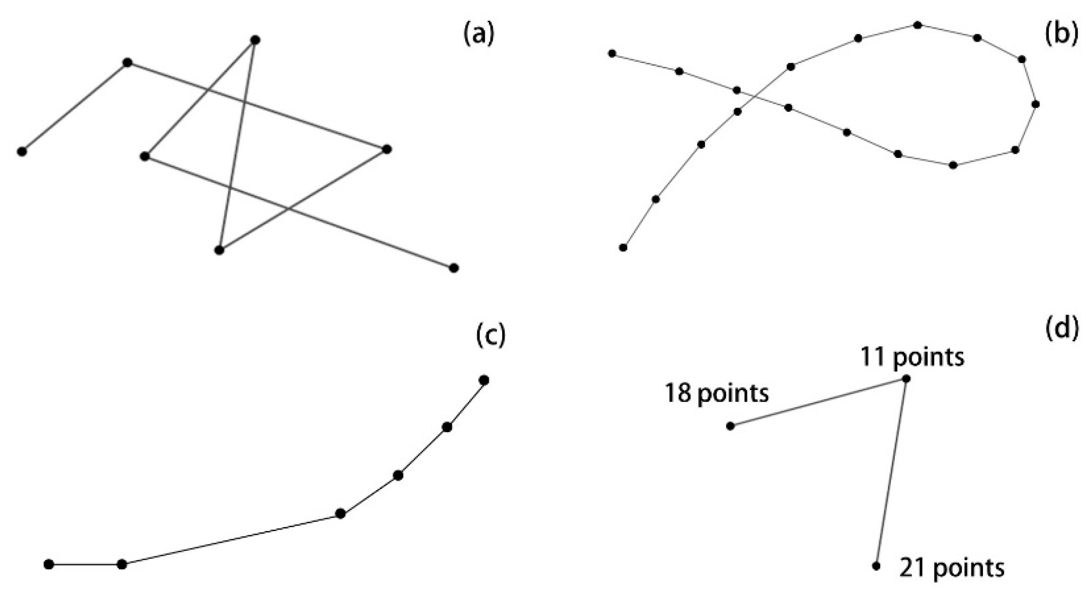
Trajectories in the evaluation set were manually labeled as either normal or anomalous by jointly considering the statistical characteristics of derived features and their visual representations. Trajectories showing linear movement with minimal directional change and short stop durations were labeled as normal, whereas those with extreme values in speed or angular variation were flagged as potential anomalies. Among these, trajectories exhibiting abnormal patterns—such as repetitive movement within confined spaces or prolonged stationary periods—were confirmed as anomalous through visual inspection. The labeling results were cross-validated by eight fellow researchers, and only the cases with full agreement were retained. The final evaluation dataset comprised 500 trajectories, including 100 anomalous and 400 normal cases. Representative examples of anomalous trajectories are presented in Figure 3, illustrating looped paths, abrupt directional shifts, and extended stationary durations—distinct from normal trajectories that traverse directly without interruption.

3.3.2. Model Architecture and Training Workflow

The proposed anomaly detection framework comprises three primary modules (Figure 4). First, the data transformation module converts raw trajectory data into input format suitable for the VAE network. Second, the reconstruction module implements the VAE to compress input trajectories into latent space and reconstruct them, enabling calculation of reconstruction error. Third, anomaly detection module determines anomalies by setting a threshold based on reconstruction errors. Trajectories with errors exceeding the threshold are classified as anomalous.
(1)
Data Transformation Module
In the data transformation module, a sliding window technique was applied to convert trajectory data into a format suitable for model input. The sliding window method divides continuous time-series data into fixed-length sub-sequences by specifying window size and stride, thereby segmenting the trajectory into smaller units. As a result of this process, each window is transformed into a high-dimensional feature vector, composed of the number of time steps multiplied by the number of features. This approach captures fine-grained temporal variations within each trajectory, allowing the model to reflect not only point-level characteristics but also dynamic patterns that emerge from sequential movement. An example of segmented trajectories using a window size of 3 and a stride of 1 is shown in Figure 5.
To normalize differences in units and value ranges across features, two scaling methods—min-max normalization and standardization—were compared to prevent training distortion and improve model convergence. This preprocessing step is essential to prevent learning distortion caused by scale disparities between variables and to enhance the model’s convergence speed.
(2)
Reconstruction Module
In the reconstruction module, a VAE-based encoder–decoder structure was employed. The encoder takes as input a trajectory segment X , obtained by dividing the original trajectory into fixed-length windows (where T is the number of time steps and F is the number of features), and compresses it into a probabilistic distribution of latent variables z (with d denoting the dimension of the latent space). Specifically, the encoder estimates the mean and standard deviation of the Gaussian distribution for the latent variable based on the input, as expressed in Equation (1). Here, f μ · and f σ · denote neural networks that output the mean and log-variance of the latent Gaussian distribution, respectively. The latent variable z is sampled from this distribution via the reparameterization trick, as shown in Equation (2). In this process, random noise sampled from a standard normal distribution is added to the latent representation, enabling gradient propagation through the stochastic layer during training. The decoder then reconstructs a segment X ^   of the same length and feature dimension as the input, representing the model’s approximation of a normal movement pattern.
The VAE is trained using an objective function composed of two loss terms. The reconstruction loss L r e c o n measures the difference between the input segment X and its reconstruction X ^ , typically computed as the mean squared error (MSE), as shown in Equation (3). The regularization term, the Kullback–Leibler divergence loss L K L , quantifies the extent to which the latent distribution q z X   inferred by the encoder diverges from a predefined standard normal prior p z , as defined in Equation (4). In this term, μ j and σ j represent the mean and standard deviation of the j -th latent dimension, respectively. This KL divergence acts as a regularizer that constrains the latent space to follow a Gaussian distribution, thereby enhancing the model’s generalization capability. The final loss function is defined as a weighted sum of these two components, and the model is trained to minimize this combined loss ( L t o t a l = L r e c o n + L K L ).
By iteratively encoding and reconstructing trajectory segments rather than entire trajectories, the model learns a probabilistic representation of normal behavior in the latent space. Normal segments cluster within high-density regions of the latent distribution, whereas anomalous segments are located in low-density areas and yield significantly higher reconstruction errors. Consequently, trajectories that deviate from learned normal patterns are more likely to produce large reconstruction errors and are thus detected as anomalies.
μ = f μ S i ,     l o g σ = f σ S i
z i = μ i + σ i × ϵ i   ,           ϵ ~ N 0 ,   1  
L r e c o n = S i S ^ i 2
L K L = D K L [ q z S i ) p z = 1 2 j μ j 2 + σ j 2 l o g σ j 2 1
where
  • S i : Input trajectory segment
  • μ : Mean of latent variable
  • σ : Standard deviation of latent variable
  • z i : Sampled latent variable
  • ϵ i : Noise sampled from standard normal distribution
  • S ^ i : Reconstructed segment
  • p z : Prior distribution
  • q z S i : Posterior distribution inferred by encoder
(3)
Anomaly Detection Module
In the anomaly detection module, reconstruction errors are calculated per segment and aggregated per trajectory. Since the VAE is unsupervised, the anomaly threshold must be manually defined. In this study, thresholds were set by visualizing the reconstruction errors and identifying the point at which the slope of the error curve stabilizes. This inflection point served as an empirical threshold for separating normal and anomalous trajectories.

3.4. Anomaly Detection and Analysis

The trained model was applied to the entire dataset to detect anomalies. As in training, preprocessed feature vectors were fed into the model, and reconstruction errors were computed for each segment. These errors were aggregated per trajectory and compared against the threshold to classify anomalies. The threshold was again determined by identifying the point where the error curve plateaued.
Anomalous trajectories were then clustered into distinct behavioral types using a clustering algorithm. Subsequently, the spatiotemporal characteristics of each cluster were analyzed, including contextual factors such as time of day and weather conditions.

4. Experiments

4.1. Experimental Setup

4.1.1. Data

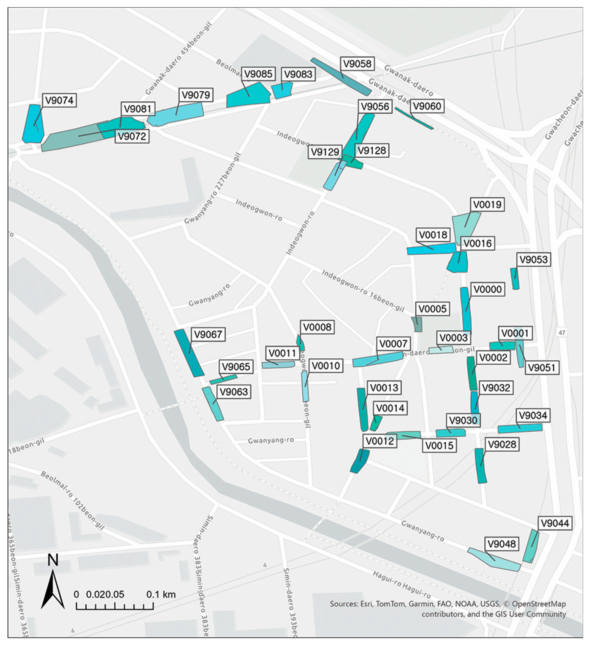
The trajectory data used in this study were collected from CCTV cameras installed near Indeogwon Station in Anyang City, Gyeonggi Province, Republic of Korea. As illustrated in Figure 6, the data were obtained from 38 CCTV locations, most of which are situated in back streets without clear separation between pedestrian and vehicular lanes. Each CCTV covers an approximately 30-m section of road. Data collection was conducted in three phases. The coverage includes 12 back streets in commercial areas, 12 back streets in residential areas with ground-level cafés and restaurants, 5 major roads, and 9 narrow alleys in residential zones with physically separated sidewalks.
The first dataset was used for model training, while the second and third datasets were used for anomaly detection and spatiotemporal analysis (Table 2). Pedestrian trajectory data consist of time-ordered sequences of location points recorded at 1-s intervals, capturing the continuous flow of pedestrian movement. A single trajectory comprises one or more points, and each point includes a CCTV identifier (sensor ID), object identifier (ID), timestamp (tm), latitude (x), and longitude (y). To ensure privacy protection, all trajectories were fully anonymized at the data-collection stage. The raw CCTV videos were processed through an automated object-tracking algorithm that distinguishes pedestrians, vehicles, and personal-mobility (PM) devices. Only the anonymized positional information of moving objects was converted into real-world coordinates at 1-s intervals and stored in the dataset. As a result, no personally identifiable information such as age, gender, or appearance attributes is included, and it is impossible to trace any individual. The dataset therefore complies with ethical standards and involves no privacy or data-protection concerns.
Short trajectories with fewer than five points were removed, as they were deemed insufficient for capturing meaningful movement patterns. As a result, approximately 52% of trajectories and 3.75% of points were removed from the first dataset; 43% of trajectories and 10% of points from the second; and 39% of trajectories and 9% of points from the third. After preprocessing, the final datasets comprised 295,798 trajectories and 26,489,737 points for training, 1,139,276 trajectories and 22,851,688 points for the second phase, and 743,711 trajectories and 15,765,593 points for the third. Subsequently, 14 movement features were extracted. Locations with unrealistically high speeds were corrected, and movement features were re-calculated based on the adjusted coordinates.

4.1.2. Evaluation Metrics

To evaluate and optimize model performance, Accuracy and F1-score metrics were employed. Accuracy was used to indicate the proportion of correctly classified samples. However, since class imbalance can inflate accuracy, it was not used as the sole evaluation metric. The F1-score, calculated as the harmonic mean of precision and recall, was adopted as the main performance indicator. It effectively reflects both false positives (normal samples misclassified as anomalies) and false negatives (missed anomalies). This metric is especially suitable for our evaluation dataset, which contains imbalanced classes. The formulas for the evaluation metrics are presented in Equations (5)–(8).
Accuracy = TP + TN TP + TN + FP + FN
Precision = TP TP + FP
Recall = TP TP + FN
F 1 = 2 × Precision × Recall Precision + Recall
  • True Positive (TP): Correctly predicted as positive.
  • True Negative (TN): Correctly predicted as negative.
  • False Positive (FP): Incorrectly predicted as positive.
  • False Negative (FN): Incorrectly predicted as negative.

4.2. Model Optimization and Performance Evaluation

Experiments were conducted by varying model parameters to evaluate the performance of the VAE-based anomaly detection model. The key parameter configurations are summarized in Table 3. The input features represent the variables used by the model for anomaly detection, while the window size specifies the number of points grouped into each segment during the sliding-window process. A feature scaler was applied to normalize differences in feature ranges, and the latent dimension determines the size of the compressed latent space.
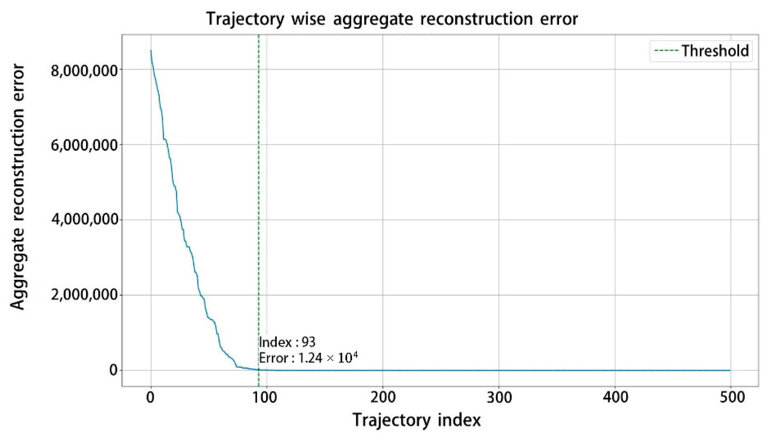
A sequential optimization strategy was adopted: starting from a baseline model, one parameter was adjusted at a time to identify the optimal configuration. The baseline model was initialized using all 14 features, a window size of 3, Min–Max scaling, and a latent dimension equal to 50% of the input dimension. The reconstruction errors of the baseline model are visualized in Figure 7. The anomaly threshold was defined at the onset of the plateau region, where variation in reconstruction error remained below 5000 for at least 100 consecutive samples. This point indicates that the reconstruction error had stabilized near zero, suggesting that all trajectory segments were reconstructed normally. Using this threshold, 94 trajectories were identified as anomalous. The baseline model achieved an accuracy of 96.80% and an F1-score of 91.67%.
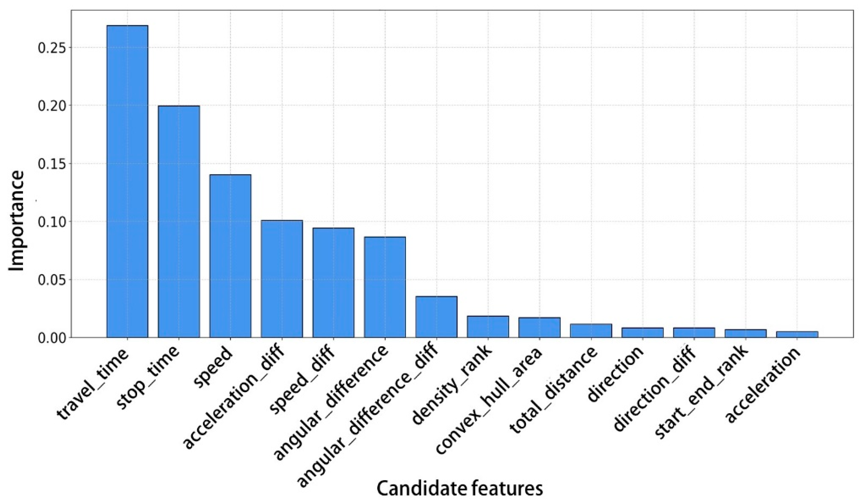
Additional experimental conditions were configured as follows. First, due to the prevalence of short-length trajectories in the dataset, window sizes from 2 to 5 were tested. Two types of data scalers—Min-Max Scaler and Standard Scaler—were evaluated. The number of latent dimensions was set to 25%, 50%, and 75% of the input feature dimension. To avoid inefficiency in testing all possible combinations of the 14 input features, they were grouped into three sets. The first group included four basic motion features: speed, acceleration, direction, and angular difference. The second group contained all 14 features. The third group was composed of key features selected based on their importance scores derived from a tree-based model. Specifically, Random Forest analysis identified six features with high importance: total travel time, stop time, average speed, acceleration difference, speed difference, and angular difference (Figure 8). Sequential optimization was performed in the order of input features, window size, scaler, and latent dimensions. The experimental settings and corresponding evaluation results for each step are summarized in Table 4.
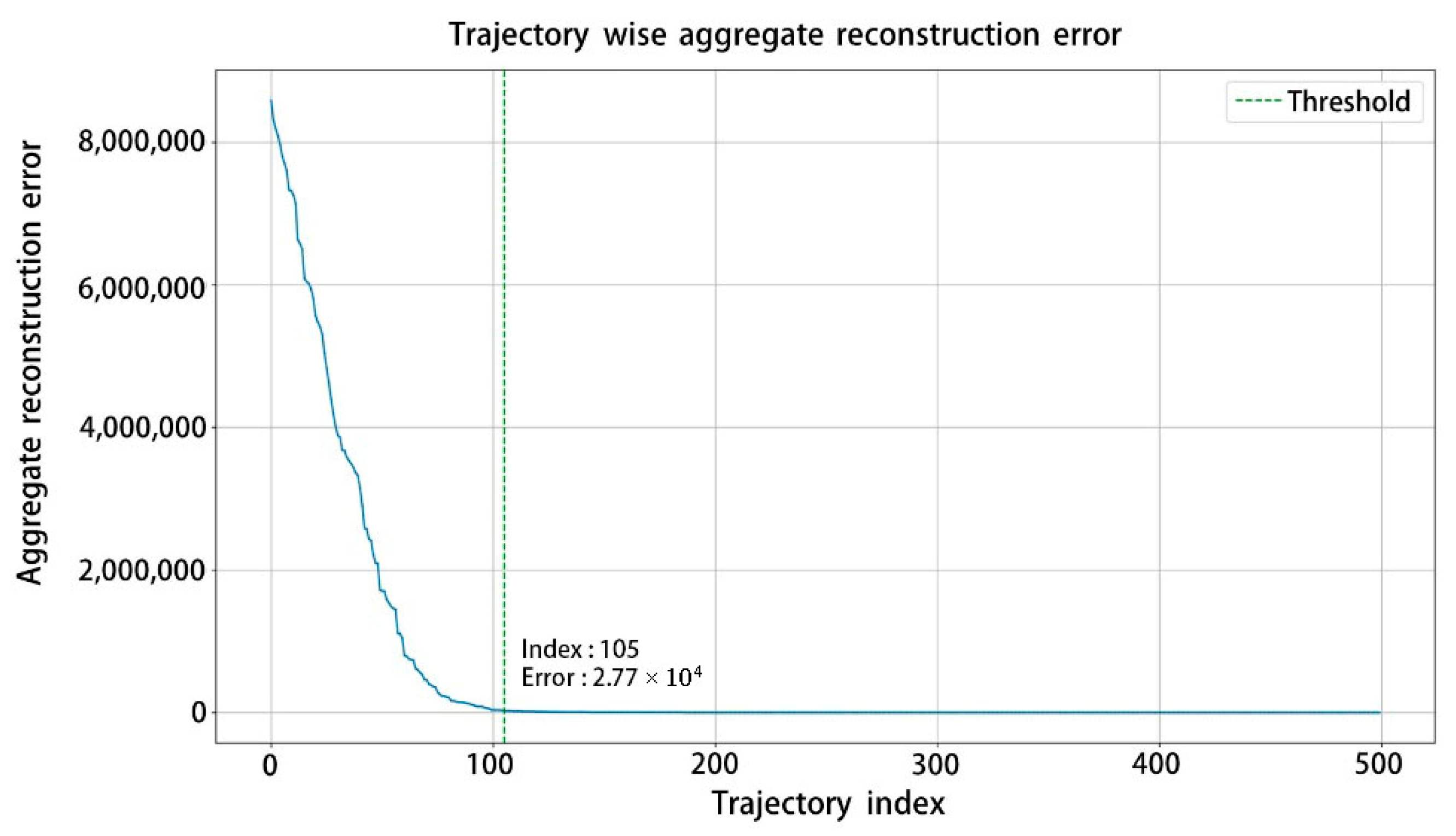
The final model achieved an accuracy of 97.80% and an F1-score of 94.63%. Figure 9 illustrates the reconstruction errors and the corresponding threshold determined using the final model. Trajectories with IDs up to 105 were identified as anomalies, with the threshold error at that point being 27,700. The threshold was defined at the onset of the stable region, where the variation in reconstruction error remained below 5000 for at least 100 consecutive samples. Under this condition, 392 out of 400 normal samples and 97 out of 100 anomalous samples were correctly classified. The improvement in F1-score compared to the baseline model demonstrates the enhanced capability of the proposed model to detect anomalies and reduce false positives. Training 5000 trajectories and detecting anomalies among 500 trajectories took approximately 62 s in a Google Colab environment using a T4 GPU. Once the model is trained, anomaly detection can be performed using the learned weights, requiring even less computation time. These results demonstrate the feasibility of the proposed method for near real-time anomaly detection.

4.3. Anomaly Detection Results

Using the final optimized model, anomaly detection was performed on the second and third datasets, comprising 1,882,987 trajectories in total. Each trajectory was input into the model to compute reconstruction errors for each segment, which were aggregated to determine anomaly scores. Thresholds were set based on the beginning of the plateau in reconstruction error graphs, where slope variation decreased, and trajectories up to that point were labeled as anomalous. As a result, 12,426 trajectories (1.09%) were detected as anomalies in the second dataset, and 7338 trajectories (0.60%) in the third. The total number of anomalies detected across both datasets was 19,764, accounting for approximately 1.05% of all analyzed trajectories.

4.4. Analysis of Detection Results

4.4.1. Anomaly Type Classification

To classify the types of anomalies, we applied K-means clustering to the 19,764 anomalous trajectories. Input features were derived from latent variables generated by the VAE encoder. Two feature sets were tested: Set A included quartiles (25%, 50%, 75%), mean, maximum, and minimum values of the latent variables, while Set B included only the mean, maximum, and 75th percentile. Each trajectory was represented as a 6-dimensional (Set A) or 3-dimensional (Set B) feature vector, followed by normalization.
K-means clustering was applied with cluster sizes ranging from k = 3 to 6. Cluster validity was assessed using two metrics: First, the Silhouette Score evaluates both cluster cohesion and cluster separation. Scores near 1 indicate well-separated clusters, while scores below 0 suggest poor clustering. Second, the Davies–Bouldin Index (DBI) measures the ratio of within cluster scatter to between cluster separation, where lower values indicate better clustering. Table 5 summarizes the results. Using set A with k = 3 yielded the best performance: a silhouette score of 0.63 and a DBI of 0.69. This configuration resulted in Cluster 0 (4644 trajectories), Cluster 1 (12,514), and Cluster 2 (2606).
To interpret the anomalous trajectory cluster, we analyzed the distribution of six key features—stop time, travel time, speed, angular difference, acceleration difference, and speed difference—across the identified clusters. Cluster 0 was characterized by frequent changes in direction and moderate stop durations, indicating repeated or erratic movement within a confined area. Prior studies have defined wandering behavior as loitering for more than 10 s or exhibiting irregular paths within limited spaces [39,40]. In this study, anomalies with frequent directional shifts and repetitive motion were labeled as wandering. Cluster 1 exhibited short stop and travel times, low angular deviation, and relatively slow speed. These trajectories resembled normal paths but were slower and more linear than typical pedestrian movements, and were therefore labeled as slow-linear. Cluster 2 showed long stop durations, very low speeds, and minimal directional change, representing pedestrians who remained stationary or moved slowly in a small area over an extended period. This behavior was interpreted as stationary. The detailed characteristics of each cluster are summarized in Table 6.

4.4.2. Spatiotemporal Context Analysis

To explore the contextual conditions under which different types of anomalies occur, this study extracted temporal, spatial, and environmental variables based on each trajectory’s location and timestamp (Table 7). Temporal context was defined by the hour of occurrence (0–23) and whether the event occurred on a weekday (coded as 1) or weekend (0). Spatial context included the CCTV identifier and characteristics of the surrounding environment. Road types were categorized into four classes: back streets in commercial areas (0), back streets in residential areas (1), major roads (2), and narrow alleys with physically separated sidewalks (3). The presence of nearby facilities—such as schools, lodging facilities, and parks—was recorded using binary indicators (0 = presence, 1 = absence). Environmental context was derived from official meteorological records, with weather conditions on the day of each trajectory categorized into four types: clear (0), rain (1), snow (2), and cloudy or foggy (3).
Using these variables, we analyzed the distribution of anomaly types across different contextual settings to identify when and where specific types of anomalous pedestrian behavior were more likely to occur. The temporal distribution of anomaly types showed that slow-linear anomalies (Cluster 1) were more prevalent during nighttime hours, particularly after 8 p.m., and were less common in the morning and early afternoon (Figure 10 Wandering anomalies (Cluster 0) exhibited slightly lower frequencies between 3 a.m. and 5 a.m., with a gradual increase afterward. Stationary anomalies (Cluster 2) showed a distinct peak during early morning hours between midnight and 6 a.m., followed by a steady decline throughout the day. No substantial differences were observed in the distribution of anomaly types between weekdays and weekends.
Table 8 presents anomaly types according to spatial context. In terms of spatial context, wandering anomalies were found to be highly concentrated in residential back streets located near lodging facilities. For instance, in zones covered by CCTVs 9032 and 9034, over 90% of the detected anomalies were of the wandering type, and these zones were located in residential neighborhoods with nearby accommodations. Slow-linear anomalies were frequently observed in back streets, but they were not detected near schools or lodging facilities. Interestingly, they appeared more often near parks, except for one zone. Stationary anomalies were more prevalent on major roads and near schools, and they were also observed in certain areas near lodging facilities, although to a lesser extent. In contrast, these stationary patterns were generally rare in areas adjacent to parks.
Lastly, the distribution of anomaly types was examined according to weather conditions (Table 9). Weather conditions also exhibited noticeable differences across anomaly types. Slow-linear anomalies were less frequently detected on rainy days and showed a significant decrease under cloudy or foggy weather. Wandering anomalies occurred less frequently when it snowed, but their frequency was highest under cloudy or foggy conditions. Similarly, stationary anomalies appeared less frequently on clear or snowy days and were more common under cloudy or foggy weather.
Taken together, these results suggest that each anomaly type is shaped by a unique set of contextual factors. Slow-linear trajectories are more likely to occur at night, wandering behavior tends to increase after dawn and is prominent in areas with lodging facilities, and stationary patterns are concentrated in the early morning hours and more common near schools and on major roads. Environmental conditions also influence the prevalence of anomaly types, with cloudy and foggy weather associated with increased occurrence, especially for wandering and stationary anomalies. These findings indicate that anomalous pedestrian behavior is context-sensitive and that specific types of anomalies tend to emerge under particular spatiotemporal and environmental conditions. The insights derived from this contextual analysis can inform strategies for urban management, public safety enhancement, and risk-sensitive surveillance.
Moreover, the use of a VAE-based model is particularly suitable for capturing subtle irregularities in trajectory-level statistical distributions. Although the most prominent anomaly types identified in this study appear as stationary, wandering, or slow-linear behaviors, their latent representations span a continuous spectrum that is not easily separable using rule-based or clustering methods. The VAE’s ability to learn low-dimensional manifolds and quantify reconstruction errors allows it to flexibly distinguish normal and anomalous patterns without hardcoded thresholds. This capability is crucial in complex pedestrian environments such as back streets, where contextual variations are subtle and behaviors are inherently diverse.

5. Conclusions

With the increasing importance of pedestrian safety in complex urban environments, detecting and understanding abnormal movement patterns has become a critical task in smart city management. Although trajectory-based anomaly detection has been extensively studied in domains such as vehicles, aircraft, and maritime transport, research focusing on pedestrian movement—particularly within unstructured environments like narrow back streets—remains limited. This study addressed this gap by proposing a VAE-based pedestrian anomaly detection framework tailored to the complexity of alleyway environments, where erratic and context-sensitive behaviors are common.
The proposed framework processes pedestrian trajectories derived from CCTV footage, extracts multi-scale motion and contextual features, and employs a VAE for unsupervised anomaly detection. Trained on real-world data and evaluated against a manually labeled dataset, the model achieved high performance with an accuracy of 97.80% and an F1-score of 94.63%. When applied to a large-scale dataset, approximately 1.05% of trajectories were identified as anomalous and further classified into three behavioral types—wandering, slow-linear, and stationary—based on latent space patterns. These anomalies showed distinct spatio-temporal and environmental characteristics, such as increased frequency near lodging facilities or during foggy weather, suggesting practical relevance for urban safety monitoring.
In addition to the high detection accuracy, this study emphasizes the rationale for adopting a VAE-based architecture over simpler rule-based methods. Although some of the identified anomaly types—such as stationary or wandering—may seem straightforward, they emerged not from predefined motion thresholds but from latent deviations learned through unsupervised modeling. The VAE was able to detect subtle irregularities like erratic stop-and-go movement, looping behavior, and meandering patterns, which are difficult to capture with heuristic filters or speed thresholds. Furthermore, the VAE framework offers scalability and generalizability, allowing it to adapt to varying urban contexts or feature configurations without the need for manual redesign. This modeling flexibility is particularly valuable in dynamic and data-scarce environments such as narrow urban alleys, where behavioral patterns are often complex and highly context-sensitive.
The novelty of this study lies in its advancement of pedestrian anomaly detection by addressing limitations of existing approaches in three interconnected ways. First, unlike prior works that primarily focus on structured road networks or vehicular trajectories, this study targets unstructured urban back street environments, where pedestrian behaviors are more erratic and context-sensitive. Second, it integrates multi-level movement features and fine-grained contextual grids into a VAE-based unsupervised framework, allowing for more interpretable and flexible detection of anomalies without relying on pre-defined heuristics. Third, the study goes beyond binary classification, offering a nuanced categorization of latent anomaly types and linking them to their spatio-environmental correlates, thereby enabling practical insights for urban safety planning. These methodological innovations build upon and extend recent developments such as uTRAND’s probabilistic anomaly clustering approach [9] and VAE-SVM hybrid methods for sidewalk hazard detection [17], but distinguish themselves by applying fully unsupervised modeling to large-scale CCTV pedestrian data and embedding context-aware behavioral interpretation within real urban alley environments.
Despite its contributions, this study has several limitations that should be addressed in future research. First, contextual information related to surrounding entities—such as vehicles or personal mobility devices—was not incorporated, limiting the model’s capacity to understand pedestrian–traffic interactions. Second, due to data anonymization, demographic attributes such as age and gender could not be considered. Third, the relatively short segment length of each trajectory—resulting from single-camera tracking—may have restricted long-term behavioral analysis. Fourth, although a 4 × 6 spatial grid was employed for extracting localized contextual features, future work should explore the impact of varying grid resolutions on detection performance in heterogeneous environments. Lastly, integrating multimodal sensor data—such as LiDAR, radar, or Bluetooth-based proximity logs—may enhance context-awareness and enable the detection of more complex behaviors, including group movement or pedestrian–vehicle interactions.
In conclusion, this study presents a scalable, context-aware anomaly detection framework that contributes to proactive and data-driven urban safety management. By leveraging deep unsupervised learning and spatio-temporal analysis, it advances the methodological landscape of pedestrian anomaly detection and offers practical tools for identifying and interpreting behaviors indicative of social vulnerabilities or safety concerns in dense urban back street environments

Author Contributions

For Conceptualization, Juyeon Cho; Methodology, Software, Validation, Formal Analysis, Juyeon Cho; Data Curation, Juyeon Cho and Youngok Kang; Writing—Original Draft Preparation, Juyeon Cho; Writing—Review & Editing, Youngok Kang; Visualization, Juyeon Cho; Supervision, Youngok Kang; Project Administration, Youngok Kang; Funding Acquisition, Youngok Kang. All authors have read and agreed to the published version of the manuscript.

Funding

This research was supported by the Korea Agency for Infrastructure Technology Advancement (KAIA) and funded by the Ministry of Land, Infrastructure, and Transport of the Korean government (Grant No. RS-2022-00143782).

Data Availability Statement

Data can be provided upon request.

Conflicts of Interest

The authors declare no conflicts of interest.

References

  1. Shi, H.; Xu, X.; Fan, Y.; Zhang, C.; Peng, Y. An auto encoder network based method for abnormal behavior detection. In Proceedings of the 2021 4th International Conference on Software Engineering and Information Management, Yokohama, Japan, 16–18 January 2021; pp. 243–251. [Google Scholar]
  2. Wang, C.; Li, K.; Chen, L. Deep unified attention-based sequence modeling for online anomalous trajectory detection. Future Gener. Comput. Syst. 2023, 144, 1–11. [Google Scholar] [CrossRef]
  3. Zhang, L.; Lu, W.; Xue, F.; Chang, Y. A trajectory outlier detection method based on variational auto-encoder. Math. Biosci. Eng. 2023, 20, 15075–15093. [Google Scholar] [CrossRef]
  4. Wang, Y.; Wang, Z.; Ting, K.M.; Shang, Y. A Principled Distributional Approach to Trajectory Similarity Measurement and its Application to Anomaly Detection. J. Artif. Intell. Res. 2024, 79, 865–893. [Google Scholar] [CrossRef]
  5. Xie, Z.; Bai, X.; Xu, X.; Xiao, Y. An anomaly detection method based on ship behavior trajectory. Ocean Eng. 2024, 293, 116640. [Google Scholar] [CrossRef]
  6. Kim, K.Y.; Kim, H.C.; Oh, S.H. Characteristic analysis of pedestrian behavior on local street in residential area. Korean Soc. Civ. Eng. D 2002, 22, 197–205. [Google Scholar]
  7. Berroukham, A.; Housni, K.; Lahraichi, M.; Boulfrifi, I. Deep learning-based methods for anomaly detection in video surveillance: A review. Bull. Electr. Eng. Inform. 2023, 12, 314–327. [Google Scholar] [CrossRef]
  8. Huang, H.; Zhao, B.; Gao, F.; Chen, P.; Wang, J.; Hussain, A. A novel unsupervised video anomaly detection framework based on optical flow reconstruction and erased frame prediction. Sensors 2023, 23, 4828. [Google Scholar] [CrossRef]
  9. D’amicantonio, G.; Bondarau, E. uTRAND: Unsupervised Anomaly Detection in Traffic Trajectories. In Proceedings of the IEEE/CVF Conference on Computer Vision and Pattern Recognition, Seattle, WA, USA, 16–22 June 2024; pp. 7638–7645. [Google Scholar]
  10. Lee, J.; Cho, J.; Kim, J.; Lee, D.; Kang, Y. Research trends analysis of vision-based trajectory prediction using deep learning. J. Korean Soc. Geospat. Inf. Sci. 2022, 30, 113–128. [Google Scholar]
  11. Zhang, D.; Li, N.; Zhou, Z.H.; Chen, C.; Sun, L.; Li, S. iBAT: Detecting anomalous taxi trajectories from GPS traces. In Proceedings of the 13th International Conference on Ubiquitous Computing, Beijing, China, 17–21 September 2011; pp. 99–108. [Google Scholar]
  12. Lin, Q.; Zhang, D.; Connelly, K.; Ni, H.; Yu, Z.; Zhou, X. Disorientation detection by mining GPS trajectories for cognitively-impaired elders. Pervasive Mob. Comput. 2015, 19, 71–85. [Google Scholar] [CrossRef]
  13. Liu, M.; Yang, K.; Fu, Y.; Wu, D.; Du, W. Driving maneuver anomaly detection based on deep auto-encoder and geographical partitioning. ACM Trans. Sens. Netw. 2023, 19, 37. [Google Scholar] [CrossRef]
  14. Kang, Y. GeoAI application areas and research trends. J. Korean Geogr. Assoc. 2023, 58, 395–418. [Google Scholar]
  15. Li, X.; Kiringa, I.; Yeap, T.; Zhu, X.; Li, Y. Anomaly detection based on unsupervised disentangled representation learning in combination with manifold learning. In Proceedings of the 2020 International Joint Conference on Neural Networks (IJCNN) 2020, Glasgow, UK, 19–24 July 2020; pp. 1–10. [Google Scholar]
  16. Yu, W.; Huang, Q. A deep encoder-decoder network for anomaly detection in driving trajectory behavior under spatio-temporal context. Int. J. Appl. Earth Obs. Geoinf. 2022, 115, 103115. [Google Scholar] [CrossRef]
  17. Guzman, E.; Howe, R.D. Sidewalk Hazard Detection Using Variational Autoencoder and One-Class SVM. arXiv 2024, arXiv:2501.00585. [Google Scholar] [CrossRef]
  18. Kolluri, J.; Das, R. Intelligent multimodal pedestrian detection using hybrid metaheuristic optimization with deep learning model. Image Vis. Comput. 2023, 131, 104628. [Google Scholar] [CrossRef]
  19. Hu, H.; Kim, J.; Zhou, J.; Kirsanova, S.; Lee, J.; Chiang, Y. Context-Aware Trajectory Anomaly Detection. In Proceedings of the 1st ACM SIGSPATIAL International Workshop on Geospatial Anomaly Detection, Atlanta, GA, USA, 29 October 2024; pp. 12–15. [Google Scholar]
  20. Suzuki, N.; Hirasawa, K.; Tanaka, K.; Kobayashi, Y.; Sato, Y.; Fujino, Y. Learning motion patterns and anomaly detection by human trajectory analysis. In Proceedings of the 2007 IEEE International Conference on Systems, Man and Cybernetics, Montreal, QC, Canada, 7–10 October 2007; pp. 498–503. [Google Scholar]
  21. Lan, D.T.; Yoon, S. Trajectory Clustering-Based Anomaly Detection in Indoor Human Movement. Sensors 2023, 23, 3318. [Google Scholar] [CrossRef]
  22. Yoon, S. Anomalous Indoor Human Trajectory Detection Based on the Transformer Encoder and Self-Organizing Map. IEEE Access 2023, 11, 131848–131865. [Google Scholar] [CrossRef]
  23. Doan, T.N.; Kim, S.; Vo, L.C.; Lee, H.J. Anomalous trajectory detection in surveillance systems using pedestrian and surrounding information. IEIE Trans. Smart Process. Comput. 2016, 5, 256–266. [Google Scholar] [CrossRef]
  24. Bera, A.; Kim, S.; Manocha, D. Realtime anomaly detection using trajectory-level crowd behavior learning. In Proceedings of the IEEE Conference on Computer Vision and Pattern Recognition Workshops, Las Vegas, NV, USA, 20–26 June 2016; pp. 50–57. [Google Scholar]
  25. Fuse, T.; Kamiya, K. Statistical anomaly detection in human dynamics monitoring using a hierarchical dirichlet process hidden markov model. IEEE Trans. Intell. Transp. Syst. 2017, 18, 3083–3092. [Google Scholar] [CrossRef]
  26. Liu, H.; Wu, C.; Li, B.; Zong, Z.; Shu, Y. Research on Ship Anomaly Detection Algorithm Based on Transformer-GSA Encoder. IEEE Trans. Intell. Transp. Syst. 2025, 26, 8752–8763. [Google Scholar] [CrossRef]
  27. Qiu, M.; Mao, S.; Zhu, J.; Yang, Y. Spatiotemporal multi-feature fusion vehicle trajectory anomaly detection for intelligent transportation: An improved method combining autoencoders and dynamic Bayesian networks. Accid. Anal. Prev. 2025, 211, 107911. [Google Scholar] [CrossRef]
  28. Shi, H.; Dong, S.; Wu, Y.; Nie, Q.; Zhou, Y.; Ran, B. Generative adversarial network for car following trajectory generation and anomaly detection. J. Intell. Transp. Syst. 2024, 29, 53–66. [Google Scholar] [CrossRef]
  29. Rezaee, K.; Rezakhani, S.M.; Khosravi, M.R.; Moghimi, M.K. A survey on deep learning-based real-time crowd anomaly detection for secure distributed video surveillance. Pers. Ubiquitous Comput. 2024, 28, 135–151. [Google Scholar] [CrossRef]
  30. Xia, D.; Li, Y.; Ao, Y.; Wei, X.; Chen, Y.; Hu, Y.; Li, Y.; Li, H. Parallel recurrent neural network with transformer for anomalous trajectory detection. Appl. Intell. 2025, 55, 519. [Google Scholar] [CrossRef]
  31. Olive, X.; Basora, L.; Viry, B.; Alligier, R. Deep trajectory clustering with autoencoders. In Proceedings of the ICRAT 2020, 9th International Conference for Research in Air Transportation, Tampa, FL, USA, 23–26 June 2020. [Google Scholar]
  32. Zissis, D.; Chatzikokolakis, K.; Vodas, M.; Spiliopoulos, G.; Bereta, K. A data driven approach to maritime anomaly detection. In Proceedings of the 1st Maritime Situational Awareness Workshop MSAW, Singapore, 24 January 2019. [Google Scholar]
  33. Jiao, R.; Bai, J.; Liu, X.; Sato, T.; Yuan, X.; Chen, Q.A.; Zhu, Q. Learning representation for anomaly detection of vehicle trajectories. In Proceedings of the 2023 IEEE/RSJ International Conference on Intelligent Robots and Systems (IROS), Detroit, MI, USA, 1–5 October 2023; pp. 9699–9706. [Google Scholar]
  34. Anik, B.T.H.; Islam, Z.; Abdel-Aty, M. A time-embedded attention-based transformer for crash likelihood prediction at intersections using connected vehicle data. Transp. Res. Part C Emerg. Technol. 2024, 169, 104831. [Google Scholar] [CrossRef]
  35. Chang, Y.J. Anomaly detection for travelling individuals with cognitive impairments. ACM SIGACCESS Access. Comput. 2010, 97, 25–32. [Google Scholar] [CrossRef]
  36. Zhao, Q.; Shi, Y.; Liu, Q.; Franti, P. A grid-growing clustering algorithm for geo-spatial data. Pattern Recognit. Lett. 2015, 53, 77–84. [Google Scholar] [CrossRef]
  37. Shi, L.; Wang, L.; Zhou, S.; Hua, G. Trajectory unified transformer for pedestrian trajectory prediction. In Proceedings of the IEEE/CVF International Conference on Computer Vision, Paris, France, 2–6 October 2023; pp. 9675–9684. [Google Scholar]
  38. Westny, T.; Olofsson, B.; Frisk, E. Diffusion-based environment-aware trajectory prediction. arXiv 2024, arXiv:2403.11643. [Google Scholar]
  39. Wahyono Harjoko, A.; Dharmawan, A.; Adhinata, F.D.; Kosala, G.; Jo, K.H. Loitering Detection Using Spatial-Temporal Information for Intelligent Surveillance Systems on a Vision Sensor. J. Sens. Actuator Netw. 2023, 12, 9. [Google Scholar]
  40. Nunez, J.; Li, Z.; Escalera, S.; Nasrollahi, K. Identifying Loitering Behavior with Trajectory Analysis. In Proceedings of the IEEE/CVF Winter Conference on Applications of Computer Vision, Waikoloa, HI, USA, 3–8 January 2024; pp. 251–259. [Google Scholar]
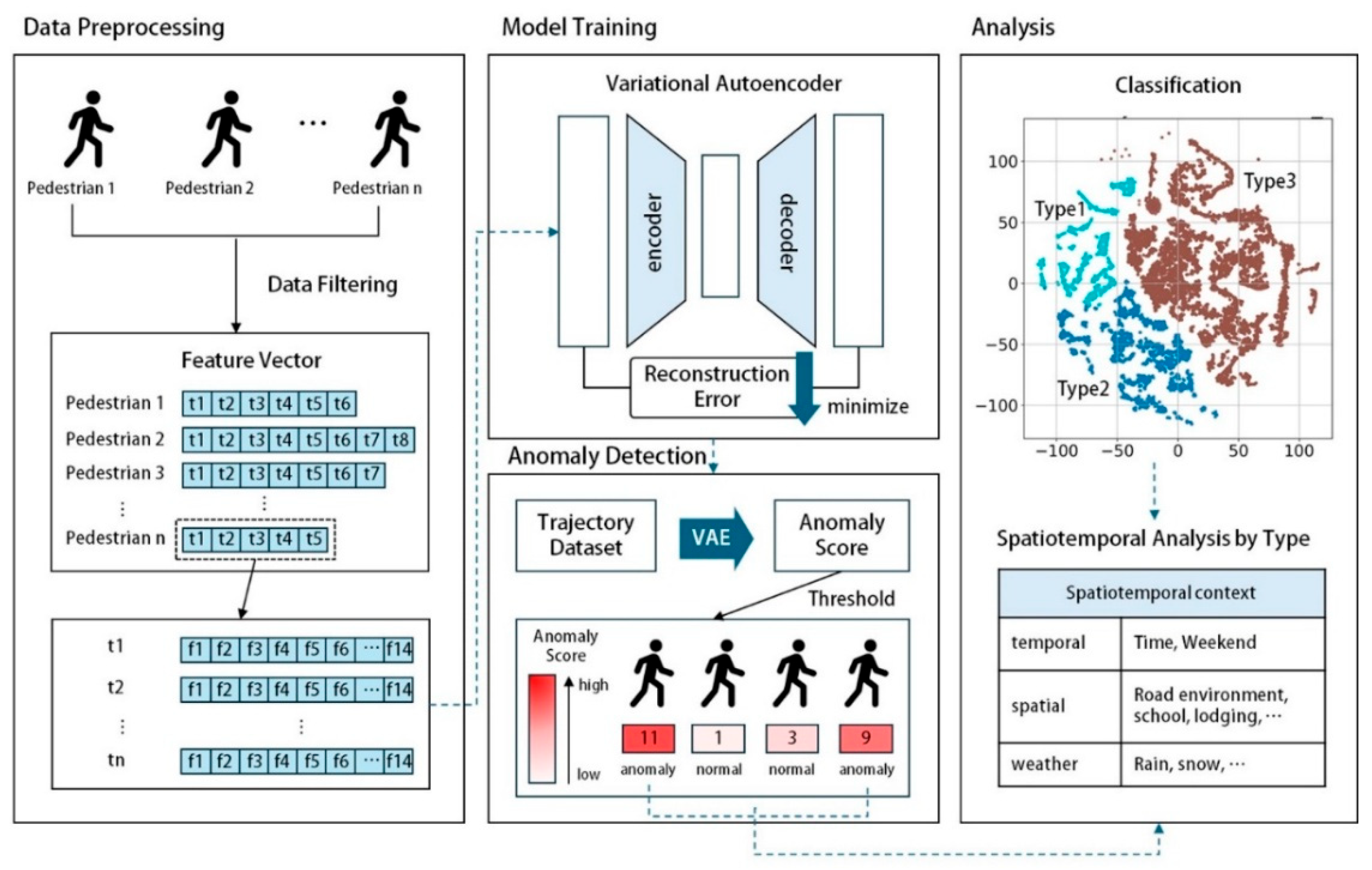
Figure 1. Research flowchart for anomaly detection of pedestrian trajectories.
Ijgi 14 00438 g001
Figure 2. Definition of the collected pedestrian trajectory data.
Ijgi 14 00438 g002
Figure 3. Examples of anomalous trajectories: (a) sharp turn, (b) loop, (c) acceleration, (d) consecutive stop.
Ijgi 14 00438 g003
Figure 4. Architecture of the VAE-based anomaly detection framework.
Ijgi 14 00438 g004
Figure 5. Segmentation of pedestrian trajectories using the sliding window technique.
Ijgi 14 00438 g005
Figure 6. Study area and CCTV location.
Ijgi 14 00438 g006
Figure 7. Threshold setting of the baseline model.
Ijgi 14 00438 g007
Figure 8. Results of feature importance analysis.
Ijgi 14 00438 g008
Figure 9. Threshold setting of the final model.
Ijgi 14 00438 g009
Figure 10. Proportion of anomalous trajectory clusters by time of day.
Ijgi 14 00438 g010
Table 1. Description of the 14 extracted features for anomaly detection.
CategoryFeatureDescription
Point-wise
Movement
Features
SpeedDistance between two points divided by time interval; indicates pedestrian speed.
AccelerationChange in speed between two points divided by time; indicates acceleration or deceleration.
DirectionAngle between two points relative to north; ranges from 0° to 360°.
Angular DifferenceAbsolute difference between consecutive directions; indicates direction change.
Global Trajectory-level FeaturesTravel DistanceThe total length of the path traveled by the object.
Travel TimeTotal duration of the movement.
Stop TimeTotal time during which speed is zero.
Convex Hull AreaThe area of the smallest convex polygon enclosing all points.
Grid-based
Features
Density RankPoints counted per grid; ranks grids from lowest to highest density (1 to 4).
Start-End RankCounts start/end points per grid; ranks grids from lowest to highest (1 to 4).
Speed DifferenceDifference between average grid speed and individual point speed.
Acceleration
Difference
Difference between average grid acceleration and individual point acceleration.
Direction
Difference
Difference between average grid direction and individual point direction.
Angular
Difference Change
Difference between average grid angular difference and individual point angular difference.
Table 2. Overview of pedestrian trajectory data collected across three phases.
RoundCollection PeriodNumber of
CCTVs
Number of
Trajectories
Number of Points
12023.09.20. 00:00:00
–09.26. 11:59:59
16616,24627,520,631
22023.12.06. 12:00:00
–12.20. 16:59:59
122,011,10525,435,082
32024.05.20. 18:00:00
–05.27. 12:59:59
381,225,02317,426,458
Table 3. Experimental settings for model performance evaluation.
Experimental ConditionDescription
Input FeaturesSet of features used by the model for anomaly detection
Window SizeLength of the temporal segment
ScalerMin-Max scaler, Standard scaler
Number of Latent DimensionsNumber of dimensions in the low-dimensional latent space
Table 4. Performance evaluation by experimental settings.
Number of
Input Features
Window SizeScalerNumber of Latent
Dimensions
AccuracyF1-Score
4---92.0075.00
62Min-Max397.8094.63
6
9
12
Standard-96.0090.91
3--97.6093.34
4--97.0092.23
5--97.0092.23
14---96.8091.67
Table 5. Clustering performance with varying feature sets and cluster numbers.
Feature Combination & KSilhouette ScoreDBI
Set A, K = 30.630.69
Set A, K = 40.590.98
Set A, K = 50.391.13
Set A, K = 60.371.12
Set B, K = 30.600.71
Set B, K = 40.510.74
Set B, K = 50.510.92
Set B, K = 60.520.84
Table 6. Characteristics of each anomalous trajectory cluster.
ClusterLabelCharacteristicsNumber of Trajectories
0WanderingFrequent changes in direction and moderate stop duration4644
1Slow-linearShort travel and stop durations
Angular difference similar to normal trajectories
Slower speed than normal trajectories
12,514
2StationaryProlonged stopping and very slow movement
Minimal directional changes
2606
Table 7. Context variable definitions for analyzing anomalous trajectory clusters.
Context TypeVariableDescription
Temporal
Context
TimeCategorical variable indicating the hour of the day (in hourly intervals)
WeekendBinary variable indicating whether it is a weekend (Sat/Sun: 0, Weekday: 1)
Spatial
Context
CCTV IDCategorical variable representing the unique identifier of the CCTV camera
Road TypeCategorical variable classifying road types into four categories:
alleyway–Commercial: 0, alleyway–Residential: 1, arterial road: 2, narrow road with sidewalk: 3
SchoolBinary variable indicating the presence of a nearby school (Yes: 0, No: 1)
LodgingBinary variable indicating the presence of accommodation facilities (Yes: 0, No: 1)
ParkBinary variable indicating the presence of a nearby park (Yes: 0, No: 1)
Environmental ContextWeatherCategorical variable representing daily weather conditions (Clear: 0, Rain: 1, Snow: 2, Cloudy/Foggy: 3)
Table 8. Analysis of anomalous trajectory clusters by spatial context.
CCTV IDWandering
(Cluster 0)
Slow-Linear
(Cluster 1)
Stationary
(Cluster 2)
Road TypeSchoolLodgingPark
000018.3478.383.260XXO
00018.6290.311.050XXX
00029.7688.381.840XXX
000316.1182.541.340XXO
00058.9186.834.240XXO
000711.9383.314.750XXX
00087.5592.440.001XXX
00106.9891.911.101XXX
00117.6391.600.761XXX
001233.3337.0329.621XXX
001310.8479.519.631XXX
001414.3476.379.281XXX
001528.5760.7110.711XXX
001621.3473.075.570XXX
001821.5664.4314.000XXX
001910.2586.972.760XXX
902875.000.0025.001XOX
903055.750.0044.241XOX
903295.650.004.341XOX
903492.850.007.141XOX
904438.180.0061.812XXX
904812.760.0087.233XXX
905173.140.0026.852XXX
905374.060.0025.932XXX
905667.720.0032.270XXX
905875.320.0024.672XXX
906071.420.0028.572XXX
906360.000.0040.003XXX
906573.910.0026.081XXX
906713.330.0086.663XXX
907227.270.0072.723OXX
907438.460.0061.533OXX
907922.750.0077.243OXX
908132.000.0068.003OXX
908317.640.0082.353XXX
908526.520.0073.473XXX
912818.7369.4111.840XXX
912951.480.0048.510XXO
Cluster 0, 1, 2: proportion values; Road type: 0 for ‘small road—commercial area’, 1 for ‘small road—residential area’, 2 for ‘main road’, and 3 for ‘narrow road with separated sidewalk’; School, Lodging & Park: “O” indicates the presence of the corresponding facility along the backstreet segment, while “X” indicates its absence.
Table 9. Analysis of anomalous trajectory clusters by weather condition.
TypeClearRainSnowCloudy/Foggy
Wandering
(Cluster 0)
12.517934.2
Slow-linear
(Cluster 1)
83.771.397.745.1
Stationary
(Cluster 2)
3.811.73.320.8
Disclaimer/Publisher’s Note: The statements, opinions and data contained in all publications are solely those of the individual author(s) and contributor(s) and not of MDPI and/or the editor(s). MDPI and/or the editor(s) disclaim responsibility for any injury to people or property resulting from any ideas, methods, instructions or products referred to in the content.