1. Introduction
In the ongoing digitalization process of smart cities and territorial space governance, multi-source heterogeneous vector data is accumulating at an exponential rate. However, the consistent expression across scales and semantics remains a key bottleneck. To achieve spatiotemporal integrated governance and business collaboration, it is necessary to reliably identify the polygon corresponding relationships of the “same real entity” under different scales and mapping standards, thereby supporting downstream tasks such as data fusion, temporal update, and change detection [
1,
2,
3]. Compared with linear features, polygons exhibit more significant shape generalization, boundary displacement, and variations in the hole and multipart structures during scale changes, resulting in the complex corresponding relationships of homonymous objects, such as 1:1, 1:M, and M:N [
4,
5,
6]. Therefore, constructing a polygon matching method that can characterize geometric–topological–semantic contexts and adapt to scale differences is of great significance for improving the consistency and timeliness of multi-source GIS databases [
7,
8].
The early research on map merging proposed a matching and registration framework based on heuristic rules, laying the foundation for object-level matching [
1,
2]. The area overlap index was first used to handle such problems [
9]. In terms of the geometric similarity measurement, the calculation indicators of the geometric similarity include position, size, shape, orientation, etc., and matching is achieved by calculating the comprehensive similarity [
10,
11], but its effect in multi-scale matching is still unsatisfactory [
12]. To address the one-to-many and many-to-many matching problems caused by scale differences, recent studies have gradually focused on “multi-scale”-oriented object context modeling and hierarchical/cognitive matching strategies. For example, multi-to-many building-/land-parcel-corresponding relationships are identified through neighborhood context aggregation and iterative optimization [
13]; the matching accuracy of building polygons under scale transformation is improved by combining Minimum Bounding Rectangle Combinatorial Optimization (MBRCO) with geometric–topological indicators [
14]. The matching problem is transformed into a classification problem, with precision, recall, and F1-score adopted as training metrics. Bayesian optimization is utilized to adjust the model hyperparameters and determine each feature threshold [
15]. Reference [
16] extracts precise topological relationships from the data for the certification of irregular tessellations. Additionally, other studies have conducted a spatial relationship analysis from both the meso-spatial scale and micro-spatial scale [
17]. In the field of road networks and other linear networks, ideas such as Voronoi diagrams, hierarchical clustering, and Summation of Orientation and Distance (SOD) comprehensive indicators have been used for multi-scale network matching, reflecting the comprehensive constraint idea of “geometry + structure + context” [
18,
19,
20], and their multi-scale modeling logic provides important enlightenment for polygon feature matching. Some studies have systematically compared various matching methods to distinguish between “reconstruction” and “replacement” and discussed the impact of different geometric metrics and thresholds on the conclusions [
21]. Other studies have proposed a direct “image-vector”-coupled road fusion framework [
22], providing a new data and constraint channel for cross-source/cross-scale matching.
However, relying solely on geometric or topological features makes it difficult to distinguish objects with a “similar appearance but different semantics” in heterogeneous data. Therefore, fusing the attribute semantic information (such as name, category, etc.) has become an important direction for improving the accuracy and interpretability of matching [
23,
24,
25]. For example, Reference [
26] established a geographic entity semantic similarity measurement model based on multi-feature constraints for road matching. Reference [
27] introduced Term Frequency–Inverse Document Frequency (TF-IDF) to calculate the dynamic weights of feature attributes and proposed corresponding similarity algorithms according to different types of feature attributes. In recent years, the application of machine learning and embedded semantic representation has further promoted the development of this field. By learning geometric–semantic joint feature vectors, transferable matching on a larger range of datasets has been realized [
28], confirming that the fusion of geometry and semantics can improve the adaptability of methods to cross-scale, multi-source, and cross-modal data, which is an important development direction in the future.
The current research still has limitations in two aspects: First, the utilization of attribute semantics is insufficient. The existing semantic similarity calculations mostly rely on standardized attributes such as names, codes, and categories [
29]; however, due to the inconsistent production standards for data, the attribute structures of the data from different sources are inconsistent, making it difficult to calculate the semantic similarity, as shown in
Table 1, which makes it difficult to deal with non-standardized descriptions, cross-lingual labels, or differentiated semantic attributes, limiting the mining of the potential of semantic information. The context-pre-trained language models in the field of natural language processing (such as BERT) have strong complex semantic representation capabilities. The Sentence-BERT model, especially, optimized by contrastive learning can achieve better semantic matching through the sentence vector cosine similarity calculation [
30,
31]. Introducing it into multi-source object matching in GIS is expected to break through the limitations of traditional methods and improve the modeling ability of complex attribute semantics.
Second, although the existing studies have conducted differentiated processing for 1:1, 1:M, and M:N matching relationships, such research still remains as the collation and optimization of traditional methods [
28]. For machine-learning approaches, due to the varying complexity of features across different matching relationships, the corresponding feature thresholds and weights ought to differ. However, no model has yet achieved differentiated modeling for these matching relationships. Other studies offer methods that can be drawn upon. For instance, Reference [
32] employs a three-branch structure with top-down and lateral connections, fusing features from different layers of the backbone network, which effectively enhances the detection accuracy for objects of varying scales in object detection. Reference [
33] dynamically selects “expert” sub-networks via a gating network to process inputs, adaptively allocating computing resources based on data characteristics, thereby reducing redundant computations and improving the model capacity. These studies validate multi-branch structures for multi-dimensional tasks, inspiring the design of a three-branch network to adapt to complex matching scenarios.
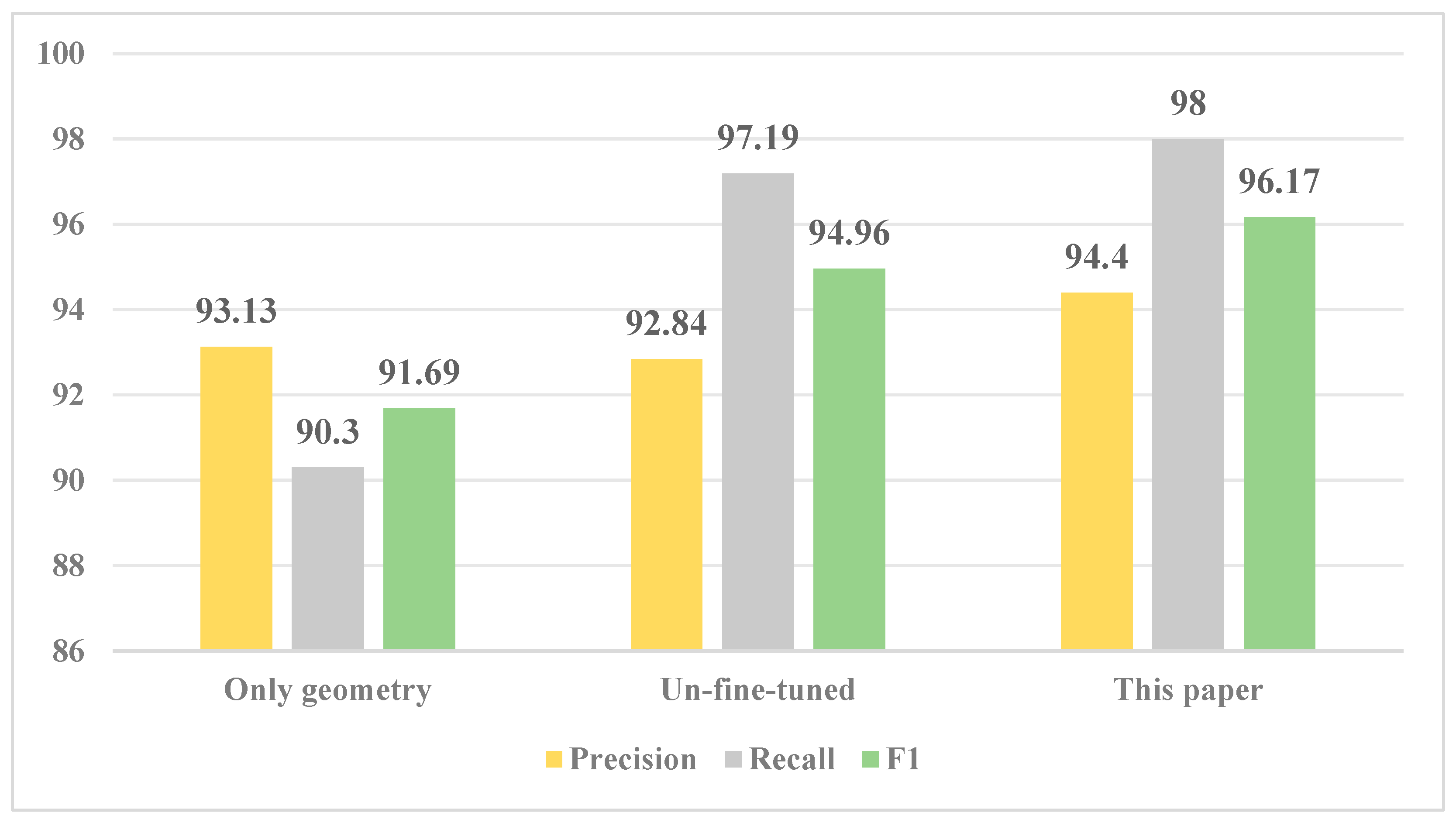
To address the above problems, this paper proposes a multi-scale polygonal entity geometric–attribute collaborative matching method based on Sentence-BERT and the three-branch attention network. To solve the problem of insufficient attribute utilization, the pre-trained Sentence-BERT model is fine-tuned to deeply mine the semantic information of complex attributes such as non-standardized descriptions, accurately calculate the semantic similarity of polygonal entities, and break through the limitations of traditional methods that rely on standardized attributes and simple comparison indicators. To solve the problem of no differentiated modeling for matching relationships such as 1:1, 1:M, and M:N, first, the matching types are divided based on polygon intersection relationships, and then the shape, size, orientation similarity, spatial overlap, and semantic similarity under different types are calculated in a targeted manner, and, finally, a three-branch network based on the attention mechanism is constructed to realize the specialized classification processing of various matching relationships, adapting to the differences in the feature complexity of different relationships. The structure of this paper is arranged as follows:
Section 2 introduces the dataset and elaborates on the proposed method,
Section 3 shows the experimental design and results,
Section 4 discusses the method, and, finally,
Section 5 summarizes the full text.
2. Multi-Scale Polygonal Matching Method
2.1. Overall Framework of the Method
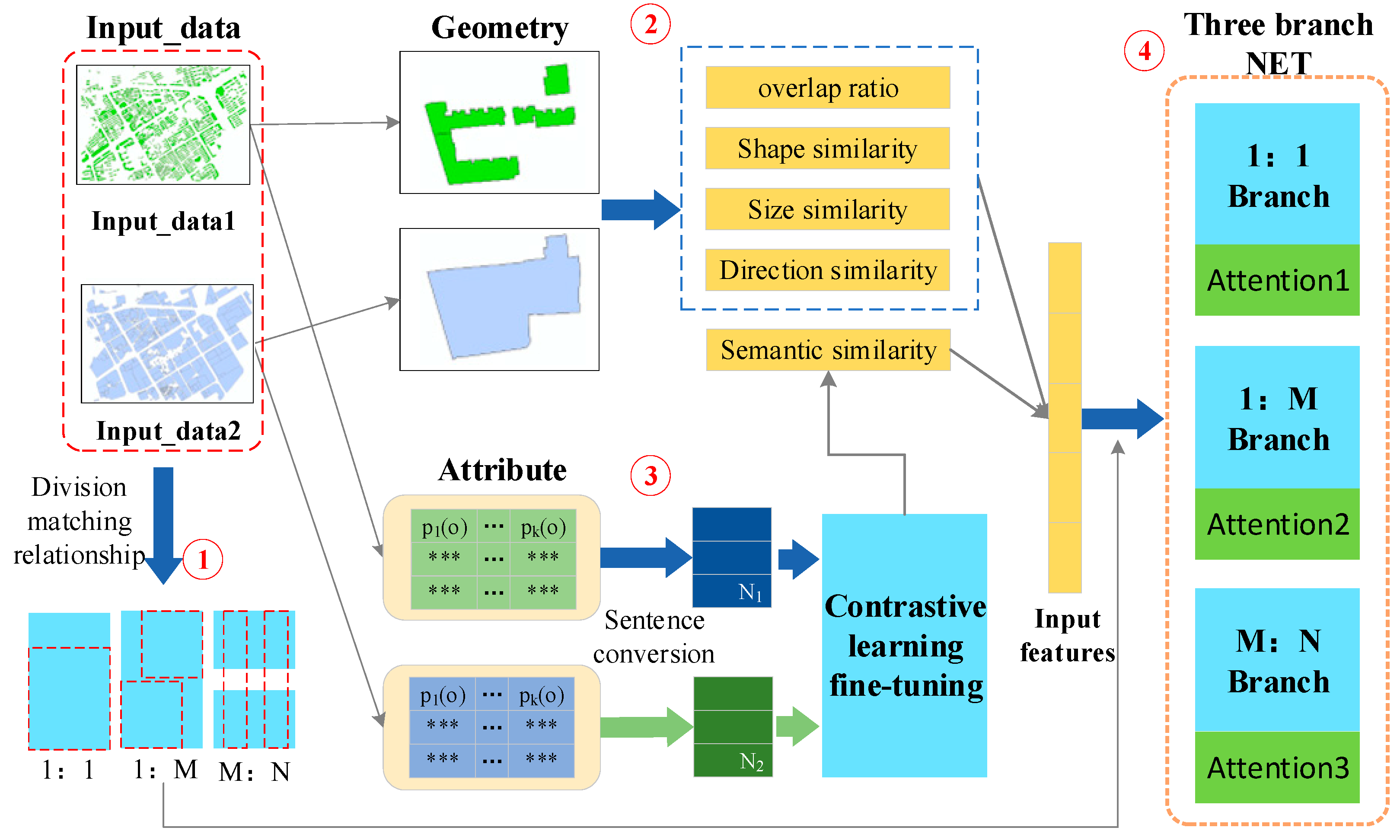
This paper proposes a geometric–attribute collaborative matching method for multi-scale polygonal entities based on Sentence-BERT and a three-branch attention network, which can calculate the semantic similarity of attributes with complex structures and adapt to various matching relationships. The method consists of four core steps, as shown in
Figure 1. First, based on the intersection relationships between polygons, the matching relationships are classified into three categories: 1:1, 1:M, and M:N. Second, for different types of matching relationships, the spatial overlap and similarities in the shape, size, and orientation of polygons are calculated, respectively. Third, the pre-trained Sentence-BERT model is fine-tuned through contrastive learning to compute the semantic similarity of polygonal entities. Finally, an attention-mechanism-based three-branch matching network is constructed to perform targeted classification processing on various matching relationships.
2.2. Subsection
The key to polygonal entity matching is to accurately identify candidate sets. The matching relationships of corresponding entities in different datasets include 1:1, 1:M, and M:N. The Minimum Bounding Rectangle (MBR) [
34], as an efficient spatial index structure, can be used for quickly filtering non-matching candidates in entity matching. When there is a position deviation in the dataset, the real spatial position of the entity may deviate from the nominal value, and matching directly based on the original coordinates is prone to misjudgment. At this time, using MBR to approximate the entity’s bounding box can effectively narrow the range of candidate sets and reduce invalid matching calculations by calculating the spatial relationship between MBRs. When there is no position deviation in the dataset, the spatial position of the entity can directly reflect its real association, and the matching logic can be constructed through the intersection relationship between polygonal entities. In this paper, entities and intersection relationships are abstracted into a graph model, and clusters are divided through the connectivity of the graph to identify matching types: Node definition: Let the set of polygonal entities in dataset A be
, and the set of polygonal entities in dataset B be
. Then, the node set of the graph is the union of the two types of entities,
. Edge definition: If there is a spatial intersection relationship between entity
and
, an edge is established between the corresponding nodes. The edge set
E is defined as the following formula:
Graph model construction: An undirected graph
is composed of node set
V and edge set
E, where the existence of edges directly reflects the spatial intersection association between entities. The connected component [
35] of graph
refers to the largest subgraph where any two nodes are connected by edges, and nodes outside the subgraph have no connection with nodes inside the subgraph. Each connected component represents a set of entities with direct or indirect intersection relationships. Let the set of connected components of graph
be
, where the
i-th cluster
can be expressed as follows:
Based on the number of entities in the cluster, the matching relationships can be divided into three categories, as shown in
Table 2:
When using intersection analysis tools to process polygonal entities, such as ArcMap or GeoPandas [
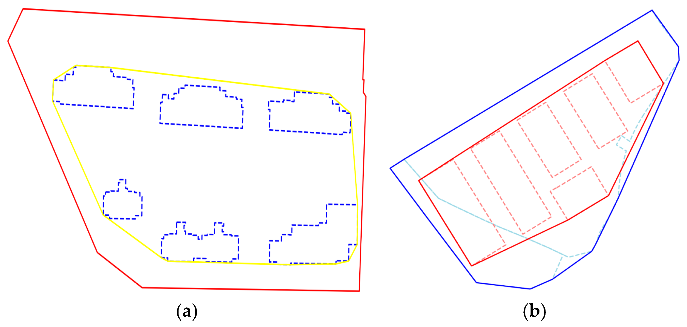
36], there are two typical misjudgment problems. First, adjacent entities with only a boundary line contact are misjudged as intersecting, but, in fact, this is only a line intersection with no area intersection, as shown in
Figure 2a; and, second, it is too sensitive to small area intersections, thus incorrectly including them in effective intersection relationships, as shown in
Figure 2b. These misjudgments will have a negative impact on the determination of candidate sets.
To this end, the model-training method adopted in this paper is as follows: by adjusting the overlap threshold, the accuracy of the candidate set under different threshold conditions is calculated. Only when the overlap of two intersecting polygonal entities reaches the set threshold will they be recorded as intersecting. Then, the threshold corresponding to the highest accuracy is determined as the input parameter of the model, so as to improve the accuracy of the model in judging the intersection relationship of polygonal entities.
2.3. Similarity of Geometric Features
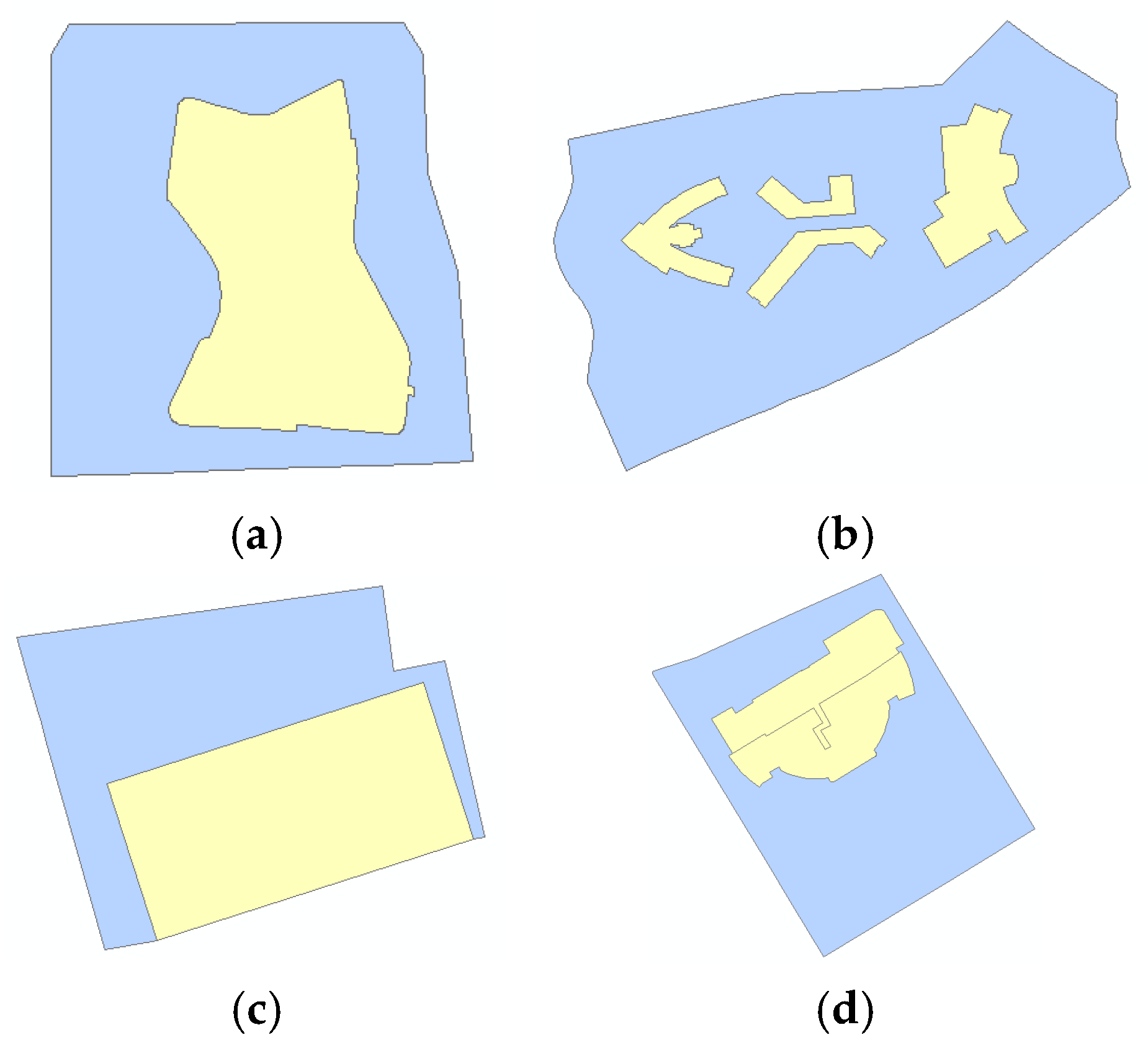
The similarity indicators of geometric features include spatial overlap, size similarity, shape similarity, and orientation similarity. The calculation methods of various indicators are very mature and have been introduced in many works of literatures. Convex hulls are used to combine multiple aggregated entities into independent surface entities to calculate the similarity, as shown in
Figure 3.
The methods adopted in this paper are as follows:
The calculation method of spatial overlap is as follows:
where
is the overlapping area, and
are the areas of the two entities, respectively.
The calculation method of the size similarity is shown in Formula (4):
where
are the areas of the two entities, respectively.
The shape similarity is calculated based on the difference in Fourier descriptors. Let
and
be the Fourier descriptors of two shapes, as shown in Formula (5):
where
n is the length of the Fourier descriptor, and
and
are the
i-th elements of
and
, respectively. The smaller the similarity value is, the more similar the two shapes are.
The calculation method of the orientation similarity is shown in Formula (6):
where
and
are the directions of polygonal entities
a and
b, respectively. Generally, the diagonal direction of the minimum bounding rectangle is used instead.
[0, 2π],
[0, 2π];
is the direction threshold, which is generally set to
=
.
2.4. Semantic Similarity
The calculation of semantic similarity adopts the framework based on Sentence-BERT [
31], and the semantic matching ability is optimized by fine-tuning the pre-trained model through contrastive learning [
37]. The overall process is shown in
Figure 4.
For entities with multi-dimensional attributes, attribute values are embedded into a natural language framework through a preset template to generate text representations that can be processed by semantic models. Let the entity set be O. For any entity o , its attribute set is expressed as , where represents the i-th attribute of entity o (such as number, name, category, location, etc.), and k is the attribute dimension.
Define the attribute-to-sentence conversion function
, which takes the entity attribute set as input and outputs the corresponding natural language sentence:
where
is the semantic sentence representation of entity o. For example, if the attributes of a dataset include name, category, and location, one of the polygons can be expressed as a sentence, as follows: “The name of Polygon 1 is China Surveying and Mapping Building, its category is ‘building’, and its location is in Beijing City.”
The pre-trained model is used to convert sentences into vector representations of fixed dimensions. For the input sentence
, the embedding vector generation process is defined as follows:
where
represents the encoding function of Sentence-BERT, and d is the embedding vector dimension (768 dimensions are used in this paper). The cosine similarity [
38] is used to calculate the semantic similarity of two sentences. For two individual entity pairs
, their similarity is defined as follows:
where
,
,
represents the vector dot product, and
represents the L2 norm.
To optimize the model’s semantic matching performance on geographic data, we select data with 1:1 matching relationships from the training data and use it to fine-tune the model, and this data contains positive and negative samples. The training data format is
, where
represents the similarity label of the sentence pair (1 for similar, 0 for dissimilar). The loss function adopts the cosine similarity loss, defined as follows:
The trained model is used to calculate the semantic similarity. The 1:1 matching relationship is directly calculated using the formula; for the 1:M matching relationship, let the source entity be , and the target entity set be . The similarity calculation follows a “entity-to-sentence-to-fused-sentence” logic: convert the source entity into a single structured sentence ; integrate all entities in the target set into one fused sentence ; and input the sentence pair , into the BERT model to compute semantic similarity, as shown in Formula (11).
The 1:M similarity calculation needs to, first, find the similarity between the source entity and each target entity, and then obtain the overall result by averaging, as shown in the following formula:
For the M:N matching relationship, let the two entity sets be
and
,
. The similarity calculation process is as follows: convert all entities in
into a fused sentence
; convert all entities in
into a fused sentence
; and input the fused sentence pair (
,
) into the BERT model to obtain the set-level semantic similarity. The specific computation is shown in Formula (12):
2.5. Three-Branch Matching Network
This paper constructs a three-branch structure to classify and process 1:1, 1:M, and M:N relationships in entity matching, and integrates the attention mechanism [
39] to realize the weight allocation. The main process is shown in
Figure 5. The three-branch network conducts differentiated learning on feature weights of different matching types through a parallel branch structure. It shares input features and common fully connected layers, thereby reducing parameter redundancy and avoiding the waste of training costs associated with independent networks.
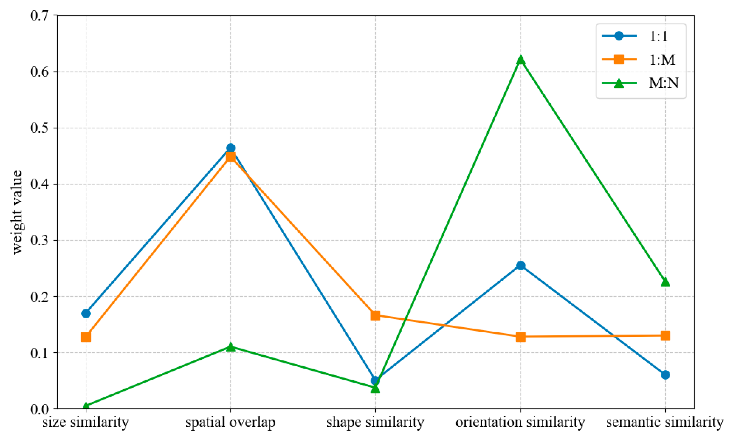
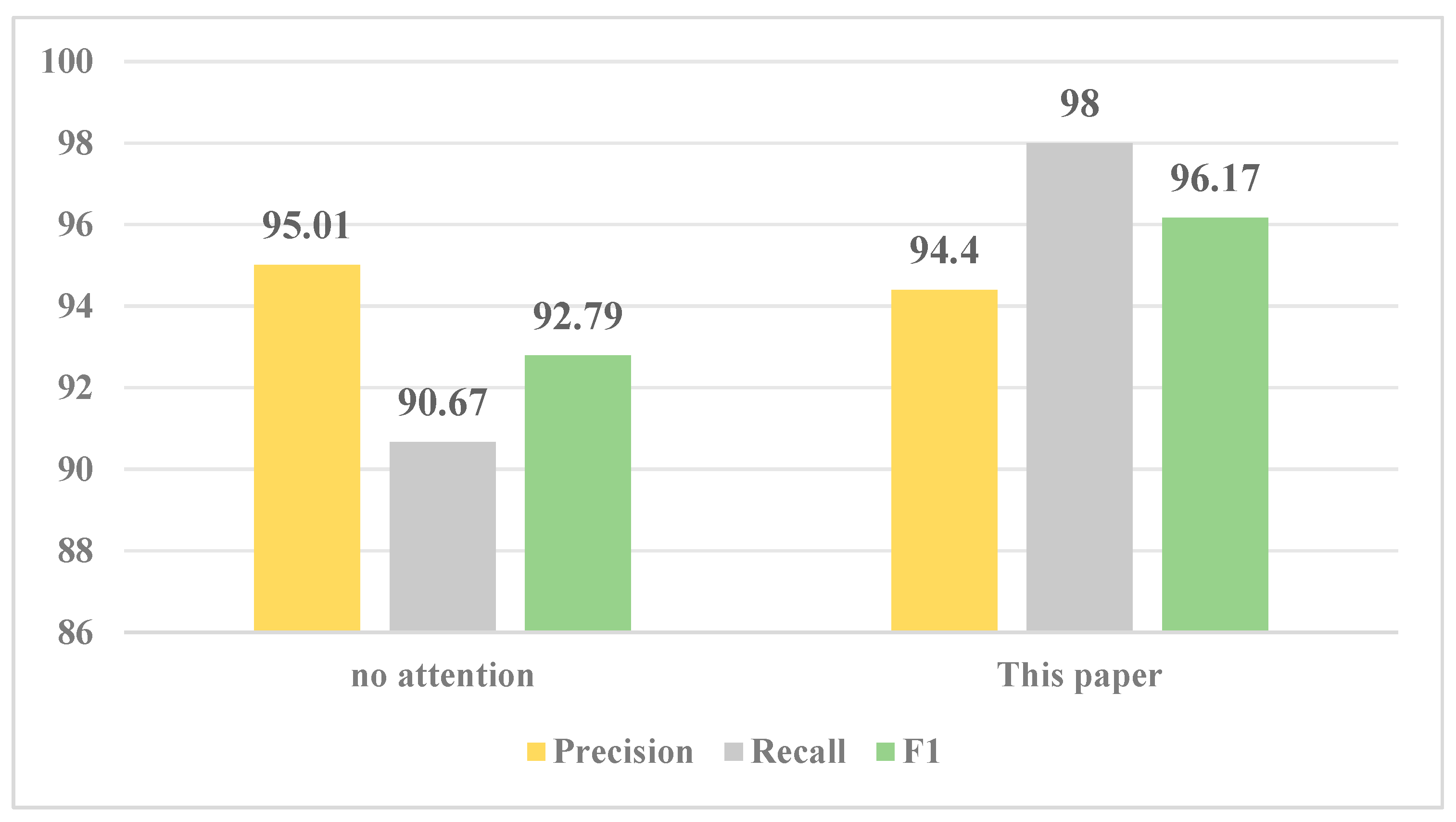
In this paper, geometric and semantic similarity indicators are used as the input of the three-branch network, and each similarity has different contributions to the matching decision. With the advantage of the attention mechanism in processing multi-dimensional data with correlation, this paper captures the correlation between indicators through adaptive weight allocation.
The attention model realizes selective attention to input features by constructing an adaptive weight matrix. The model structure includes two layers of the linear transformation and activation function.
The first layer of linear transformation maps the input features to the hidden layer space: , where is the input feature vector, is the weight matrix, and is the bias vector. The hyperbolic tangent function tanh is used as the activation function to introduce non-linear transformation: a = tanh(z). The second layer of linear transformation maps the hidden layer representation back to the input feature dimension, , where , . The softmax function is used to normalize the output to obtain the attention weight vector, , where represents the attention weight of the i-th feature.
The feature weighting process can be expressed as
, where ⊙ represents element-wise multiplication. The model is trained by minimizing the mean square error loss function, and the optimization target is Formula (14):
where
f(
) is the model prediction function,
is the
k-th sample feature,
is the target value, and
N is the number of samples. After training, the final feature attention weight
= [
,
,…,
] is obtained by averaging the attention weights of all training samples.
Each branch is equipped with an independent fully connected layer and a weight allocation module. As shown in the 1:1 branch in
Figure 5, the weight allocation module is applied to the feature
of the
i-th sample to obtain
, and linear transformation is performed through the fully connected layer
, as shown in Formula (15):
where
, and
is the bias term. The processing methods of branches 1:M and M:N are similar.
The ReLU activation function is applied to the output of each branch:
. The output of each branch after the activation function is passed into the common fully connected layer
for linear transformation,
, where
is the bias term of the common fully connected layer. The ReLU activation function is applied again to the output of the common fully connected layer:
. The output after re-activation is passed into the output fully connected layer
for linear transformation, and then the Sigmoid activation function is applied to obtain the final predicted value
, as shown in Formula (16):
where
is the bias term of the output fully connected layer.
Binary Cross-Entropy Loss (BCELoss) is used for model optimization, as shown in formula (17):
where
N is the total number of samples,
0, 1} is the true label,
is the predicted value, and the Adam optimizer is used to update parameters.
5. Conclusions
This paper presents a geometric–attribute collaborative method for multi-scale polygonal entity matching, aiming to address the limitations of insufficient semantic utilization and the undifferentiated modeling of complex matching relationships in existing approaches. The key contributions are summarized as follows:
Enhanced semantic similarity computation: By fine-tuning the Sentence-BERT model, the method effectively captures semantic information from non-standardized attributes and multi-dimensional descriptions, overcoming the constraints of traditional string-based or dictionary-based semantic comparison. This significantly improves the ability to distinguish entities with similar a geometry but different semantics.
Differentiated modeling for matching relationships: Based on a polygon intersection analysis, matching relationships are classified into 1:1, 1:M, and M:N. A three-branch attention network is designed to handle each relationship type specifically, with adaptive feature weighting via attention mechanisms. This tailored approach adapts to the varying feature complexities of different relationships, improving the matching accuracy for both simple and complex scenarios.
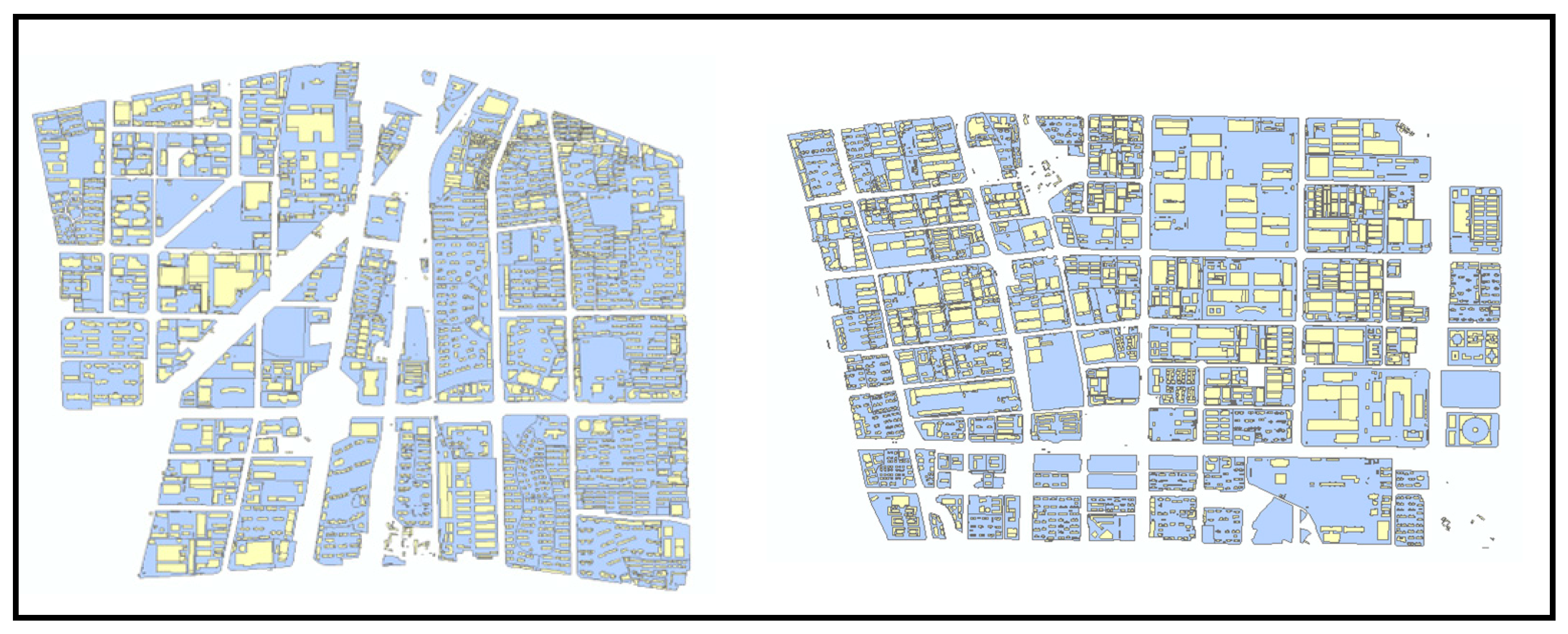
Superior performance and generalization: The experimental results on the Huangshan and Hefei datasets demonstrate that the proposed method outperforms existing geometric–attribute fusion and BPNN methods in precision, recall, and F1-score. The consistent effectiveness across different study areas confirms its strong generalization ability.
