Article

How Does Built Environment Influence Housing Prices in Large-Scale Areas? An Interpretable Machine Learning Method by Considering Multi-Dimensional Accessibility

1
Hongyi Honor College, Wuhan University, Wuhan 430072, China
2
State Key Laboratory of Information Engineer in Surveying, Mapping and Remote Sensing, Wuhan University, Wuhan 430072, China
3
School of Geography and Tourism, Anhui Normal University, Wuhu 241003, China
*
Author to whom correspondence should be addressed.
ISPRS Int. J. Geo-Inf. 2025, 14(11), 436; https://doi.org/10.3390/ijgi14110436
Submission received: 18 July 2025 / Revised: 26 October 2025 / Accepted: 1 November 2025 / Published: 4 November 2025

Abstract

The housing prices are crucial to the sustainable development of the real estate market. Nowadays, few academic attempts have focused on the impact of multi-dimensional accessibility on housing prices in a large-scale area. This study utilized machine learning methods to extract indicators of the visual environment from street view images. The indicators were combined with multiple sources of spatiotemporal geographic big data, such as second-hand housing data and online map POIs, to quantify the factors of housing prices. Both the hedonic price model and random forest were constructed, with Shapley additive explanations applied to interpret the results. Our work took Shanghai as a case study, and the results indicate that the random forest exhibits superior performance compared to the hedonic price model. The location accessibility (e.g., distance to the CBD) is paramount, and functional accessibility (e.g., to subways and finance facilities) exhibits nonlinear thresholds. We further uncovered the characteristics of the nonlinear relationship between visual environmental factors and housing prices. Our findings can deepen the understanding of housing price variation in the spatial dimension and provide the theoretical basis for ensuring the optimization of urban planning.

1. Introduction

In recent years, with the continuous advancement of urbanization, the favorable economic environment has stimulated a continuous rise in urban housing prices. Keeping the long-term, rational, and stable development of housing prices is very essential for the construction of a harmonious and healthy society. There have been numerous pieces of evidence that economic crises are triggered by the sharp fluctuations in housing prices, such as the Japanese real estate bubble in the 1980s and the US subprime mortgage crisis in 2007 [1]. Understanding the variation patterns of housing prices and deeply investigating their influencing mechanisms can promote more rational purchases and reduce blind investment. On the other hand, it can also provide a basis for decision-makers to formulate policies related to real estate and urban planning.
For decades, the topics related to housing prices have been widely discussed in the domains of urban planning [2], geography [3], and computer science [4]. Many works aimed to understand the influencing mechanism of housing values in different socioeconomic contexts. Most existing studies depend on surveys and are limited to a small area. They pointed out that the built environment is strongly correlated with housing prices [5]. The concept of the built environment originated in the fields of urban planning and architecture and generally refers to the physical space where people live [6]. Several scholars have shown that built environment factors, such as the accessibility of housing to transportation and nearby services, can influence their corresponding market value [7]. The concept of walking accessibility has been extensively studied by scholars [8]. Numerous papers have focused on the significant influence of part of accessibility to specific factors such as transportation, schools, and hospitals on residential prices [9,10,11]. However, few studies have used machine learning to systematically explore the relationship between multi-dimensional accessibility and housing prices.
Urban green space, sky, and other environmental elements are closely related to the quality of urban life [12,13]. These environmental factors can significantly influence people’s feelings. Street greenery is beneficial to the psychology and behavior of pedestrians [14,15]. Research consistently shows that the quality of the street view images around houses usually has an impact on the price of the houses. Studies in Beijing, Shanghai, and elsewhere demonstrate that higher street-level green view index (GVI) and sky view index (SVI) values generally boost nearby property values, suggesting homebuyers value these environmental features [16]. Liujia Chen et al. [17] found that the relationship between the GVI and housing prices is nonlinear, which has positive impacts on housing prices, and the sky view index has a negative influence on housing prices. Some scholars have begun to extract variables such as GVI and SVI and have confirmed that these variables are significantly correlated with housing prices.
The widespread application of street view images prompts a deep understanding of the built environment in large-scale areas. Street view products, including Google Street View and Baidu Street View, provide a detailed visual representation of urban environments from a human perspective. Street view images are characterized by extensive coverage, rich content, high resolution, and ease of access, making them valuable as supplementary data sources for urban study [18]. Nowadays, street view images have been applied to evaluate the physical environment indices, such as noise, traffic flows, and population. The development of interpretable machine learning not only increases the evaluation accuracy based on street view images but also explores the complex relationship between the built environment and physical indices. However, few scholarly attempts have focused on investigating the impact of visual environmental features on housing prices in large-scale areas by combining street view images. Evaluating the housing prices and explaining their influencing mechanism are essential for stimulating the urban economy.
To investigate the impact of multi-dimensional accessibility on housing prices and enhance the understanding of how the built environment factors affect housing prices, we proposed an interpretable machine learning framework by combining different data resources. The factors that may have an impact on housing prices are extracted from Baidu Street View images, Gaode Map, and Lianjia second-hand housing data. Both the hedonic price model and random forest (RF) were constructed to evaluate the housing price. The Shapley additive explanations (SHAP) were introduced to further detect the nonlinear relationship between the built environment and housing prices. This work can provide reference opinions for potential housing consumers, intermediaries, and relevant government departments to make decisions. Additionally, our findings have positive effects for promoting the healthy and stable development of the real estate market.

2. Related Works

2.1. Influencing Mechanism of Housing Prices

The influencing mechanisms of housing prices are complex and diverse [19,20,21,22]. Housing prices can be estimated using the hedonic pricing model, which considers structural, neighborhood, and locational attributes as key components of housing value [23,24]. Structural features refer to the properties of the house, such as area, floor, and orientation. Locational and neighborhood features mainly refer to the accessibility of the house to the surrounding infrastructure (such as the distance to the city center, transportation facilities, and education facilities). At the early stage, both the geographical location and transportation condition were found to be strongly correlated with the variation in housing prices [25]. Subway, tram, and suburban railway stations have a positive impact on housing prices, while, because of the traffic noise, national railway stations, ports, and airports are also linked with a decrease in housing prices [26]. An empirical analysis in Portland revealed that the relative direction of the central business district can influence housing prices [27]. Some scholars have investigated the contribution of various service facilities, such as schools, parks, hospitals, and restaurants, to housing prices [28,29,30,31]. Wen, et al. [32] revealed that the accessibility of educational facilities can increase the housing prices of the corresponding surrounding areas. Evidence showed that buyers and investors were willing to pay extra for the quality or accessibility of education [33]. In addition to the above factors, scholars also explored the influence of construction years, number of bedrooms or bathrooms, floor area, garage, and other architectural structural factors [34,35,36].
In recent years, visual environmental features have also been incorporated [37]. Many studies have regarded urban environments, such as vegetation, sky, roads, and buildings, as visual environmental features for evaluating housing prices [16,17]. As an important built environment factor, urban green space has many ecological benefits, such as air purification, climate regulation, carbon storage, and noise reduction [38,39]. At the same time, green space also provides residents with an open space to release pressure, which can have a positive effect on residents’ mental health [14,40]. Donovan and Butry [41] quantified the impact of trees on the rental price of single-family houses in Portland and found that planting trees on the vacant lot surrounding the house could increase the monthly rent of the house. Belcher and Chisholm [40] took Singapore as a case to study the economic value of vegetation in developed tropical cities. The sky openness has been paid much attention by many scholars [42,43]. Luttik [44] studied the transaction records of houses in eight towns and found that the houses with water features could bring a premium of 8–10%. In addition, existing studies pointed out that some landscapes may be linked to the housing prices. Jim and Chen [45] revealed the changes in housing prices in the landscape of the harbor and mountains. Their results showed that a harbor landscape can increase the price by about 3%, and the impact of a mountain landscape on housing prices is insignificant. Previous studies have identified the significant factors of housing prices effectively. However, no scholarly attempts have systematically explained the complex relationship between the built environment and housing prices in a large-scale area.

2.2. Hedonic Price Model

The examination of the real estate market has consistently garnered the interest of researchers. The existing methods can be classified into traditional and advanced methods in the field of property valuation. Traditional methods can include the comparative method, cost method, residual method, profits method, and investment method. Due to the complexity of factors influencing housing prices and the diversity of housing characteristics, these traditional approaches have limitations in reflecting the true value of housing comprehensively and accurately. As an important advanced method, the hedonic price model is the most effective approach to estimate housing prices. Koji Karato et al. [46] proposed a semiparametric hedonic model of housing prices to reveal significant nonlinearities in both the age and cohort effects and significant interactions between these effects in Tokyo between 1990 and 2008. This model is capable of assessing the influence of property attributes as well as other external factors that could affect the property value [7].
In the field of real estate, the hedonic price model is the regression of housing prices. Since Lancaster and Rosen [24,47] proposed the hedonic model theory, the application research of the model has made considerable progress. The model conceptualizes housing as a heterogeneous good. Following Rosen [24], housing prices are regressed via ordinary least squares (OLS) on three main groups of explanatory variables capturing the property’s structural, location, and neighborhood features. Traditional models have certain limitations in practical applications, such as the inapplicability of the Gaussian distribution assumption, multicollinearity issues, and the uncertainty of function form selection. However, despite these limitations, the models continue to be widely used because of their ease of use and interpretability. To address some of these limitations, researchers often apply various transformation forms in hedonic models, such as linear, semi-log, Box–Cox, and semiparametric models [46,48,49]. Among these, the semi-log form stands out as a widely used one.

2.3. Machine Learning in Street View Images Studies

Machine learning has been widely applied to extract the visual elements of the built environment from street view images. On the other hand, it is also an effective approach for evaluating physical indices or human perception based on visual elements. Existing semantic segmentation techniques can identify the visual elements and calculate the proportion of each element [18]. Yu, et al. [50] utilized the PSPNet model to obtain the semantic information of street view images and quantified an index to measure green space in urban areas. Naik, et al. [51] measured the ground, building, tree, and sky by analyzing the semantic segmentation of street view images and proposed two street view indexes to uncover the differences among block places. Chen, et al. [52] optimized the DeepLab series networks by adding the full convolution operation of FCN. The proposed method has the void convolution and pyramid pooling and can greatly improve the segmentation effect. By combining visual elements, some scholars further classified the scenario types. Song, et al. [53] used the visual element proportion as the input and then assessed the scenario accurately based on XGboost. Their results finally revealed the relationship between noise level and scenario types. Zhou, et al. [54] extracted 512-dimensional features from the Places dataset based on the ResNet model to express the overall characteristics of the scene and analyzed the visual similarity and specificity between a scene and other scenes, places, or regions.
With the support of machine learning, the physical environment indices or human perception can be evaluated and mapped in large-scale areas. In terms of human perception, it is a hot topic to introduce machine learning for quantifying happiness, depression, stress, and other emotions. Zhang, et al. [55] obtained street view images of Beijing and extracted vegetation, buildings, roads, walls, and other elements. They discussed and revealed the relationship between elements and residents’ safety and depression. Based on the map of human perception, Ramírez, et al. [56] investigated the heterogeneity of different demographic groups. The perception varied significantly with age and gender. In terms of physical environment indices, the noise, solar radiation, and pedestrian volume can be quantified accurately by combining street view images and machine learning. Yin and Wang [57] proposed a novel method for measuring road traffic noise and then employed class active mapping to visualize the interpretation of their evaluation results. Wang, et al. [58] explored the impact of street direction on solar radiation and assessed the radiation by analyzing the visual elements and solar trajectories. Wang, Hou, Zhang and He [58] conducted validation tests by comparing pedestrian volume from street view images and the reality. The quality and size of street view images have been proven to be highly correlated with the validation accuracy. To the best of our knowledge, existing research lacks an effective method of evaluating housing prices by combining street view images.

3. Study Area

This study chose Shanghai as the study area to investigate the impact of the built environment on housing prices. As one of the four direct-controlled municipalities in China, Shanghai is a major center for finance, shipping, international trade, and technological innovation. It is also one of the most economically dynamic regions in China, with the highest level of innovation and openness. The total administrative area of the city is 6340.5 square kilometers, accounting for 0.06% of the national land area. As of 2021, the built-up area covers 1237 square kilometers. Based on the results of the 7th National Census, Shanghai’s resident population is about 24.8 million, with the registered resident population at 14.4 million. Like other major cities around the world, the rapid development of the city and the growth in population are often accompanied by a sharp increase in housing prices. Between 2012 and 2021, the average housing price in Shanghai increased by 1.27 times. As a city with a net inflow of population, Shanghai’s large population and the scarcity of land have contributed to its high housing prices. According to data released by the National Bureau of Statistics in February 2022, the average housing price in Shanghai reached 67,996 yuan per square meter. The inequality and polarization of residents’ incomes in Shanghai have significantly affected their housing affordability, leading to adverse impacts on the city’s sustainable development and social stability.

4. Data Collection

The housing prices, point of interest (POI) data, and street view images in Shanghai were collected in this work. The Python 3.8 web scraping techniques were utilized to obtain the housing prices data from Lianjia, the largest real estate agency website in China. The period from 2019 to 2023 was significantly impacted by the COVID-19 pandemic. During this time, housing prices were distorted due to a combination of factors such as lockdown measures, economic uncertainty, and changes in buyer behavior. Housing prices did not accurately reflect the underlying real estate market conditions. Additionally, the data on transaction prices in China are difficult to collect. Access to actual transaction data is restricted and primarily held by the housing management departments of local governments [49]. Some real estate agencies have transaction data, but their limited market coverage results in insufficient data for comprehensive analysis. This study utilized Python web scraping techniques to obtain the housing price information of 2018 on the Lianjia website, which is the largest real estate agency website in China. The detailed information includes the district and street, neighborhood name, property type, floor level, building area, orientation, listing price, unit price, etc. The second-hand homes’ data details are shown in Table 1. After removing duplicates and incomplete records, a total of 64,346 records, which cover 8630 neighborhoods in Shanghai, were finally collected. The distribution of second-hand homes is shown in Figure 1.
POI is the term commonly used by scholars [59,60,61]. POI refers to geographical entities with particular social functions such as catering, hospitals, schools, and shopping centers. The POI data includes information such as ID, name, longitude and latitude, administrative district, category, and address. As a vital data source for analyzing urban spatial structure, the POI data are extensively utilized in research on urban planning and related disciplines. The POI data for Shanghai in 2018 was obtained from the Gaode Open API platform. The detailed information of the POI data attribute table is shown in Table 2. Based on the Urban Land Classification and Planning Standards for Construction Land, the POI data are categorized into two scales: coarse-grained and fine-grained. The classification results are shown in Table 3. The coarse-grained POI includes five categories: commerce, transportation, industry, public services, and green spaces. The fine-grained POI includes 13 categories, such as shopping, external transportation, companies, scientific research, and education.
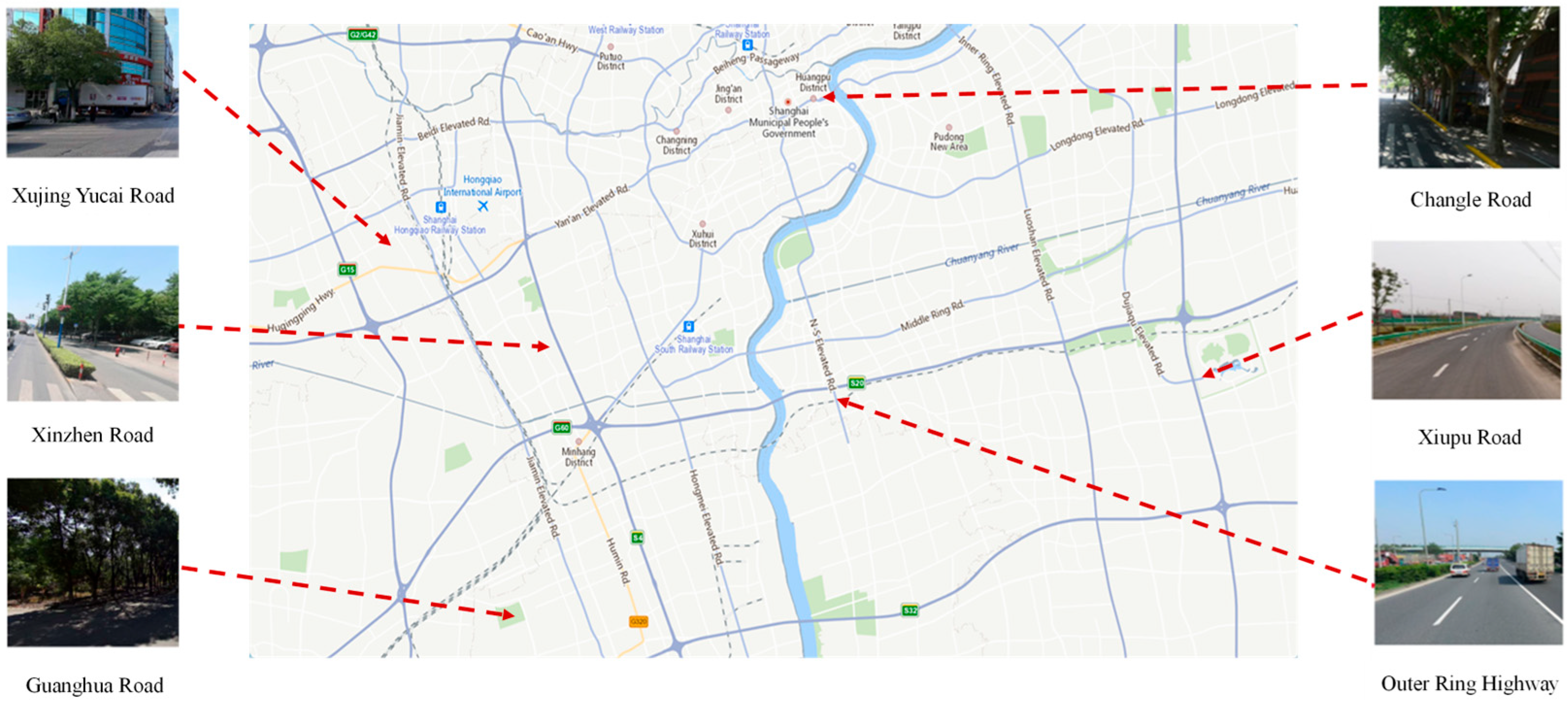
The street view images in Shanghai were collected from the Baidu Maps API. In order to better simulate the actual pedestrian perspective, we collected street view imagery configured with a 360° horizontal field of view and a 22.5° vertical pitch angle [62]. The distribution of Baidu Street View images in Shanghai is shown in Figure 2. Samples of the street view imaginary were taken at intervals of 50 m along the center line of the road, the original size is 4096 × 2048 pixels, and the image metadata include information such as ID, year, longitude, and latitude. After removing the images with missing metadata, a total of 2,218,630 street view images of Shanghai in 2018 were collected. To facilitate calculation and analysis, the different data will be unified in the same coordinate system. The integration of all data sources is matched by geographical coordinates.

5. Method

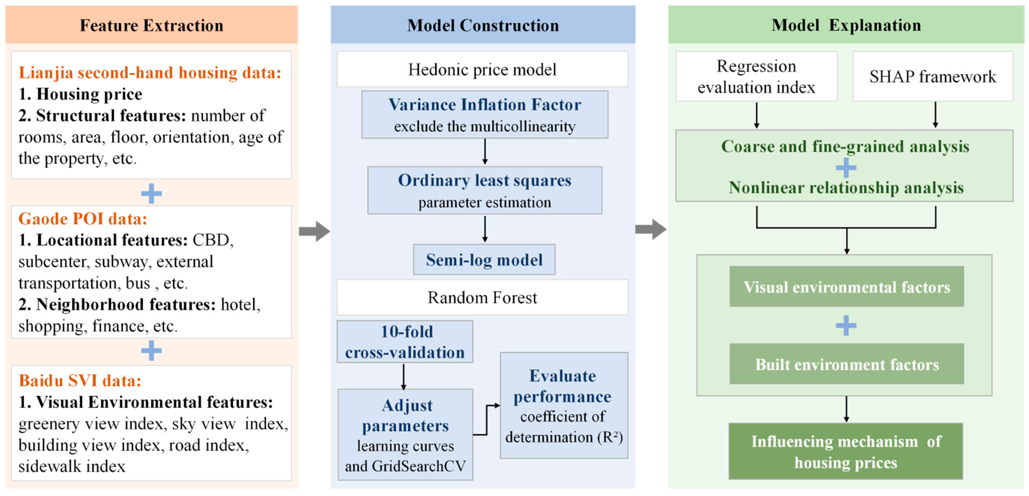
The research framework diagram is shown in Figure 3. To investigate the mechanisms influencing housing prices, we initially integrated housing transaction data from Lianjia, POI data from Gaode, and street view images from Baidu to extract relevant factors. We constructed a semi-log hedonic price model and employed an RF model combined with SHAP value analysis to identify key influencing factors and elucidate their underlying mechanisms.

5.1. Influencing Factor Extraction

The influencing factors of housing prices are extracted from the Lianjia second-hand housing data, Gaode POI data, and Baidu Street View images. The influencing factors in this work include structural, locational, neighborhood, and visual environmental features. The structural factors are extracted from the Lianjia second-hand housing data. Structural factors are a series of variables directly related to the property itself, which can reflect the physical structure of the house. In previous studies on housing prices, Sirmans, et al. [63] summarized the commonly used structural factors, including age, area, garage, bedrooms, bathrooms, swimming pool, and number of basements. Among these factors, age was mentioned frequently and had a negative impact on housing prices. This study extracts 5 structural factors of housing prices from second-hand housing data: number of rooms, area, floor level, orientation, and property age.
Locational factors are typically described by using accessibility indicators in geography, including accessibility to employment centers, major amenities, and transportation infrastructure. These factors reflect the ease of transportation within the city and the convenience of accessing important places. This study selected the distance to the central business district (CBD) as a locational factor; this factor was calculated as the Euclidean distance from the housing to People’s Square in Shanghai. Additionally, this study extracted transportation-related factors from the Gaode POI data to measure the transportation accessibility of the housing. The locational factors also include both coarse-grained and fine-grained variables. The coarse-grained factors are referred to as transportation and describe the convenience of access to various transportation facilities from the housing. At the fine-grained level, these factors were defined as the accessibility to external transportation, accessibility to bus stations, and accessibility to subway stations. In this work, transportation accessibility is calculated as the number of relevant category POIs within a 1000 m radius around the housing.
Neighborhood factors described the accessibility of the housing to various nearby amenities. Previous studies have shown that factors such as commercial amenities, landscape environment, employment opportunities, and public service facilities near housing can influence its prices [64,65]. This study extracts neighborhood factors from the Gaode POI data based on the basic principle of the 15 min living circle. A 1000 m walking distance is used as the buffer radius to calculate the number of various POIs around the housing [66]. Neighborhood features are divided into coarse-grained and fine-grained levels. At the coarse-grained level, features are extracted and quantified by using four categories of POIs: commerce, industrial, public services, and green spaces. At the fine-grained level, factors are extracted and quantified using ten categories of POIs, including shopping, companies, research and education, and public healthcare.
Visual environmental factors are the quantification of the visible surroundings of the housing. This study selected a buffer radius of 400 m based on the average area of residential communities in Shanghai. Relevant studies have also demonstrated that 400 m is approximately the square root of the average area of communities in Shanghai [17]. Based on previous studies, we obtained the environmental factors at the neighborhood level [17]. A circular buffer with a radius of 400 m was created around the centroid of its residential community to represent its visual range. Within the 400 m buffer zone, the maximum number of street view images that can be obtained is 1508, and the minimum is 59. On average, each community has 570 images. All street view image sampling points falling within this buffer were identified through spatial joining. This study employed the DeepLab v3+ network model for the semantic segmentation of street view images. The Deeplab series is a series ofm semantic segmentation algorithms developed by the Google team based on FCN [52]. DeepLabV3+ is the latest version. DeepLab v3+ adds the Xception model [67] and applies the depthwise separable convolution to both Atrous Spatial Pyramid Pooling and decoder modules, resulting in a faster and stronger encoder–decoder network. It improves the accuracy of image feature sampling. The DeepLab v3+ network has been validated in various computer vision tasks. The model was pre-trained on a high-quality street view dataset from Shenzhen, which was professionally labeled by an expert labeling company. This dataset contains annotations of 19 element categories, including greenery, sky, building, road, sidewalk, terrain, person, bicycle, motorcycle, car, traffic light, traffic sign, other signs, pole, fence, awning, trash can, overpass, and pedestrian bridge. The pixel accuracy of DeeplabV3+ in the training set and the test set reached 98.1% and 95.1%, respectively. The sky, roads, sidewalks, buildings, and greenery were selected to construct visual environmental features by considering the potential influence of various factors on housing prices. This resulted in five indicators: green view index (GVI), sky view index (SVI), Building View Index (BVI), road index, and sidewalk index. The calculation formulas for each indicator are as follows:
GVI = pixel S greenery pixel S total
In the equation, GVI represents the percentage of the greenery in the image, pixel S greenery represents green pixels in image, and pixel S total represents total pixels in the image. SVI, BVI, road index, and sidewalk index were calculated using the same procedure as GVI.
The various factors extracted in this study and their specific quantification methods are shown in Table 4. The dependent variable is the housing price, with 16 independent variables at the coarse-grained level and 24 independent variables at the fine-grained level. The descriptive statistics of the selected influencing factors are shown in Table 4.

5.2. Model Construction

This study constructed both a hedonic price model and RF to reveal how the built environment influenced the housing prices. The housing price was input as the dependent variable. The independent variables include structural, locational, neighborhood, and visual environmental features. The OLS was used as the parameter estimation method. The specific functional form is shown in Equation (2).
l n P = α 0 + a i S i + b i L i + c i N i + d i V i + ε
In the equation, P represents housing price, S i denotes the structural factor, L i represents the locational factor, N i stands for the neighborhood features, and V i refers to the visual environment factors. The a i , b i , c i , and d i are the regression coefficients of the corresponding factor in the semi-log model, respectively. α 0 is the constant term, and ε is the error term.
RF is well-suited to handle data imbalances, as well as potential issues such as missing values and multicollinearity, exhibiting strong robustness. Therefore, this study directly uses all factors as inputs for the RF model. This study builds an RF regression model based on the Scikit-learn library. Learning curves and GridSearchCV were introduced to determine the hyperparameters of the RF regressor. By utilizing all sample data from Shanghai, a learning curve was plotted between the maximum number of iterations and R2, finding that the model stabilizes when the n_estimators parameter reaches 150. In this study, the n_estimators was set to 180. GridSearchCV was utilized to identify the optimal values for max_depth, min_samples_leaf, min_samples_split, and max_features. The values of these hyperparameters are shown in Table 5. After constructing the RF regression model, the original dataset was split into training and testing sets in a 9:1 ratio. The optimal model was obtained by adjusting parameters on the training set, and predictions were then made on the testing set. To evaluate the performance of the constructed hedonic price model and RF regression model on the Shanghai second-hand housing dataset, this study used the coefficient of determination (R2) for evaluation and applied 10-fold cross-validation to prevent overfitting.

5.3. Shapley Additive Explanations

SHAP and Local Interpretable Model Agnostic Explanation (LIME) are currently the most popular explainable artificial intelligence (XAI) methods. Compared to LIME, SHAP not only provides both global and local explanations simultaneously but also reveals the positive or negative directions of the corresponding influencing factors and outputs nonlinear correlations [68,69]. A fundamental limitation shared by both SHAP and LIME is that they are inherently correlational, not causal. Additionally, SHAP is much slower than LIME, especially with tree-based models [70].
SHAP is an additive explanation framework that can be used to interpret the output of any machine learning model. The core idea of SHAP is Shapley values, which were first introduced in 1953 by the renowned American mathematician and economist Lloyd Shapley. Shapley values are primarily used to address the issue of distributing the gains and contributions in cooperative games [71]. In 2017, Lundberg and Lee from the University of Washington first proposed the SHAP framework and applied it to model interpretation, providing a solution to the conflict between the accuracy and interpretability of machine learning models [68].
The SHAP framework unifies six existing additive feature attribution methods, including LIME, DeepLIFT, layer-wise relevance propagation, Shapley regression values, Shapley sampling values, and quantitative input influence [72,73,74]. The SHAP values were used as a unified measure of feature importance. Through validation, it has been found that, compared to other methods, SHAP values better align with human cognition of model interpretability and exhibit superior computational performance.
SHAP is an additive feature attribution method, meaning that it can explain a model’s prediction as the sum of the attribution values of each input feature, as shown in Equation (3).
g z = 0 + j = 1 M j z j  
In the equation, g represents the explanation model; z { 0 , 1 } M indicates whether the feature can be observed; M refers to the number of factors; j R represents the attribution value of each factor; 0 is the constant term of the explanation model, which represents the mean prediction of all training samples. Shapley values satisfy the requirements of efficiency, symmetry, dummy, and additivity, which ensure the fair distribution of cooperative gains.

6. Results and Analysis

6.1. Spatial Autocorrelation Results Analysis

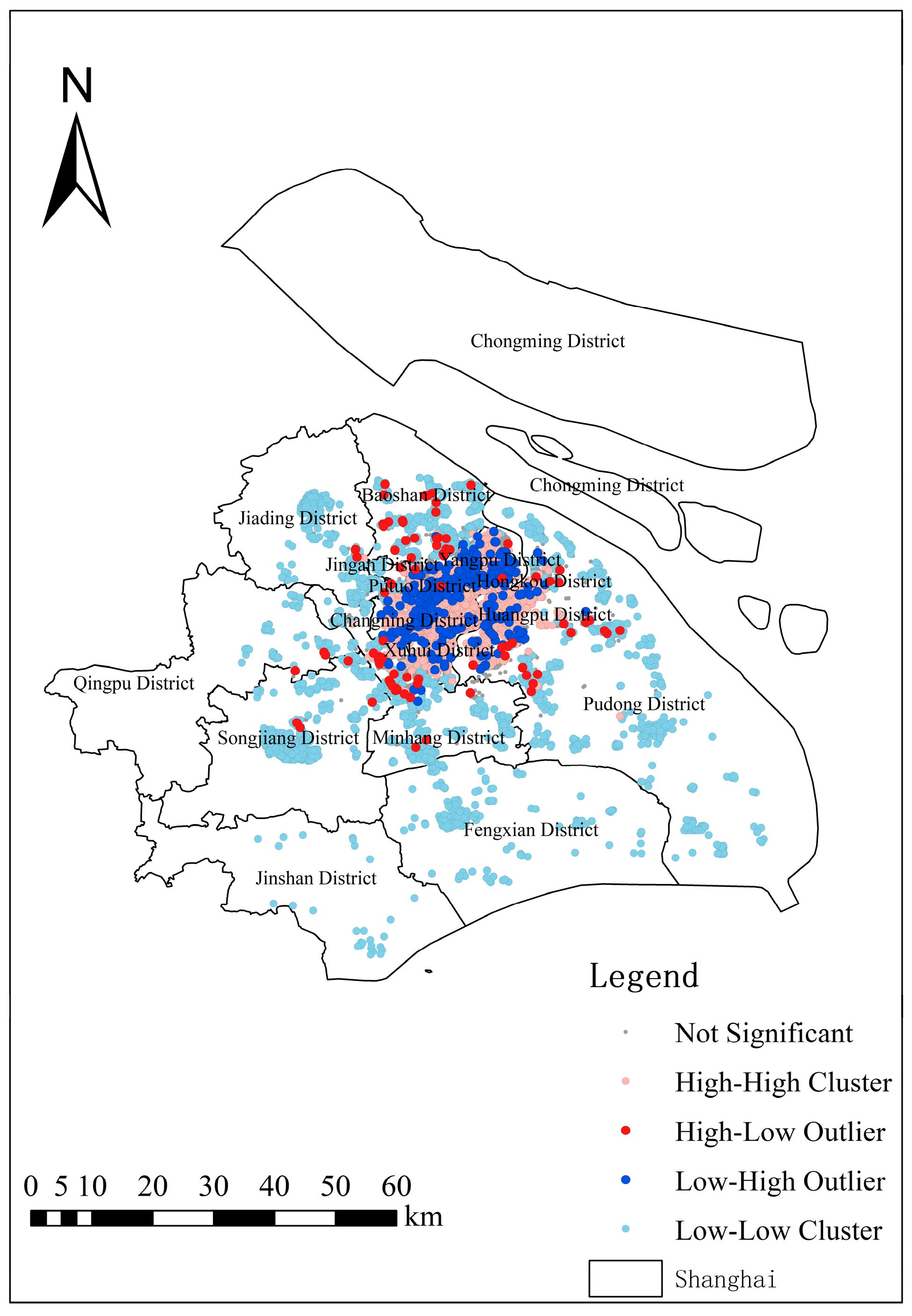
In order to reveal the spatial distribution pattern of housing prices, spatial autocorrelation analysis can be introduced. This analysis mainly utilizes the ArcGIS 10.8 to obtain the Moran’s I test results and the LISA clustering map. The global Moran’s I index was shown in Table 6. Moran’s I = 0.7993 indicates that there is a significant spatial autocorrelation in the housing price data, meaning that the housing prices in adjacent communities are similar. p < 0.001, and it, therefore, passes the 95% confidence test. Z = 690.7280. This indicates that the housing prices in Shanghai in 2018 exhibited a high degree of spatial autocorrelation, which means neighborhoods with high house prices are always adjacent to each other. The LISA cluster plots show the high-high (HH), low-low (LL), high-low (HL), and low-high (LH) phenomena with significance levels. Figure 4 shows the LISA clustering map of housing prices in Shanghai. From the perspective of spatial distribution, “HH” mainly gathers in the city center, while “LL” is the opposite, occupying a larger area.
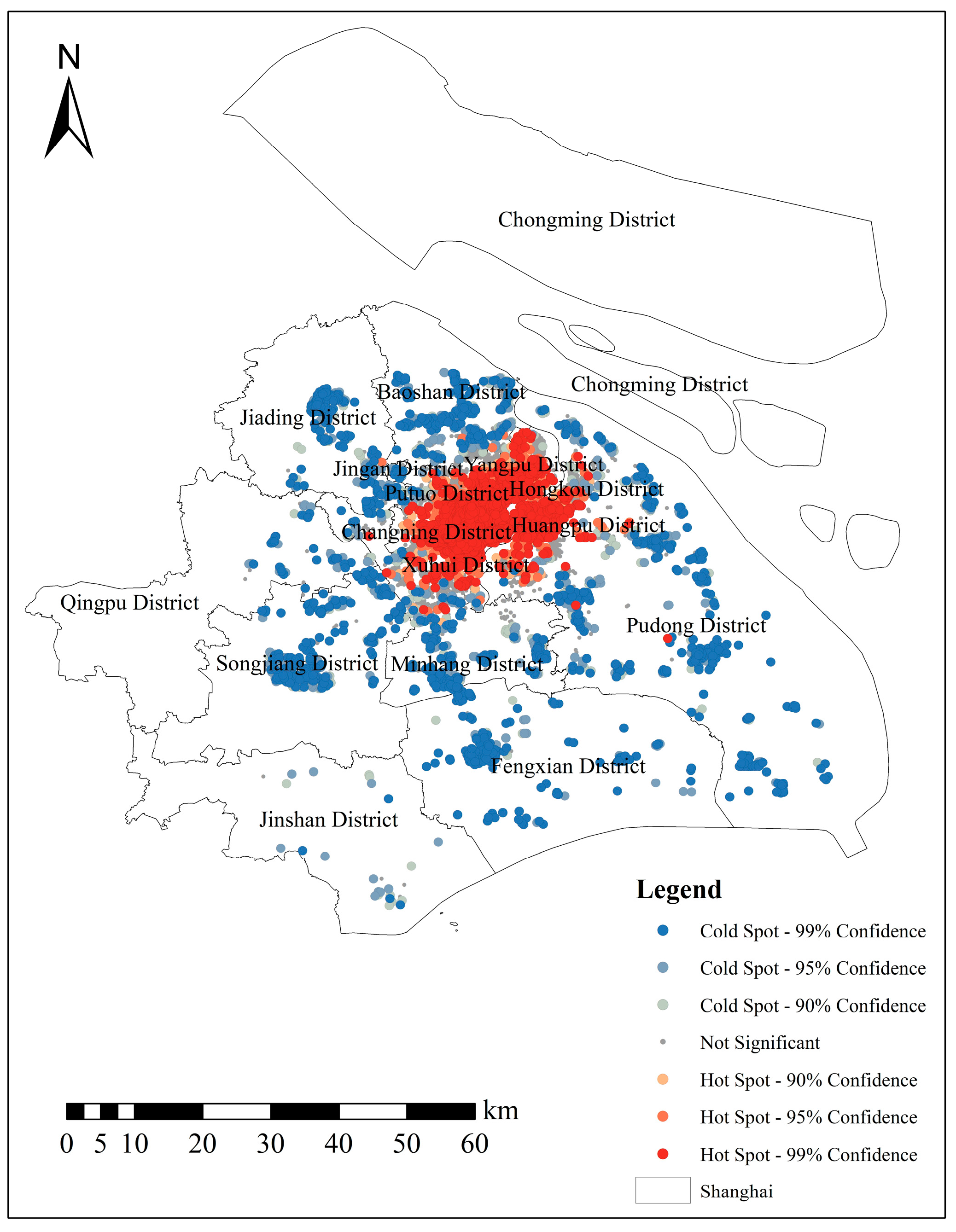
To further verify the robustness of the spatial distribution pattern of housing prices, this study also performed a hot and cold spot analysis based on the Getis-Ord Gi* statistic. Moran’s I and LISA measure spatial similarity. Compared with these, Getis-Ord Gi* statistics offer a different perspective. It no longer merely measures the clustering of similar values but can directly identify spatial clusters of significantly high and low values with statistical significance. As shown in Figure 5, housing prices in Shanghai exhibit a distinct spatial clustering pattern. The hot spots are consistently concentrated in the city center, while the cold spots are primarily distributed in the peripheral areas. This result is closely aligned with the conclusions derived from the global Moran’s I and LISA analysis presented in the main text. Collectively, the hot and cold spot analysis corroborates a high degree of spatial autocorrelation in Shanghai’s housing prices, revealing a pronounced core-periphery structure and thereby strengthening the robustness of the findings regarding spatial dependence and heterogeneity.

6.2. Hedonic Price Model Results Analysis

The coefficient of each factor in the hedonic price model was estimated based on the ordinary least squares method. The variance inflation factor (VIF) was applied to check the multicollinearity between independent factors. The coefficient, significance test, and VIF are shown in Table 7. All VIFs were lower than 10, which indicated that there is no multicollinearity among factors. All factors passed the significance tests. As shown in Table 8, at the coarse-grain level, the R2 of the hedonic price model is 0.7680. At the fine-grained level, the R2 of the model is 0.7918, indicating that the model can explain 79.18% of the information in the sample. The Root Mean Square Error (RMSE) and Mean Absolute Error (MAE) decreased from 0.1693 and 0.1287 to 0.1604 and 0.1208, respectively. According to the calculation results of the regression evaluation index, it can be preliminarily judged that the fine-grained hedonic price model has higher accuracy than the coarse-grained model. To test the sensitivity of key variables, the radius of the buffer zone has been changed, and the key variables have been recalculated using 800 m and 1200 m, respectively. As shown in Appendix A Table A1, the direction and statistical significance of the influence of the key explanatory variables have not undergone any fundamental changes. The performance of models is maintained at a relatively stable level with minimal fluctuations.
From Table 7, we have found that the distance to CBD has the greatest impact on the housing prices at both the coarse-grained and fine-grained levels. Although the weight of traffic factors is not high in the coarse-grained model, the impact of the Shanghai Metro on housing prices cannot be ignored from a fine-grained perspective. At the coarse-grained level, the impact of neighborhood factors, such as public service, industry, and green spaces, on housing prices ranks higher. Combined with the standardization coefficient of fine-grained factors, it can be found that public healthcare has a significant impact on housing prices. The more public healthcare near the housing, the higher the prices. In addition, shopping, hotel, leisure and entertainment, and other commercial facilities also have a strong correlation with housing prices, while the leisure and entertainment and housing prices showed a significant positive correlation. The results of the hedonic price model show that the contributions of the visual environment factors to the housing prices are slightly smaller among the three categories of built environment factors. The visual environment indicators include GVI, SVI, BVI, road index, and sidewalk index. The factors of GVI, road index, and BVI have a positive impact on housing prices, while BVI and sidewalk index have a negative impact.
To further verify the robustness of the model, we followed the previous methods and used two different functional forms of the hedonic price model, namely the semi-logarithmic and linear models [8]. The results are shown in Table 9. The t-values of all variables are very close, and the signs of almost all variable coefficients are also consistent. This indicates that our semi-log hedonic price model has passed the robustness test, and all variables can explain the housing prices.

6.3. Machine Learning Model Interpretation

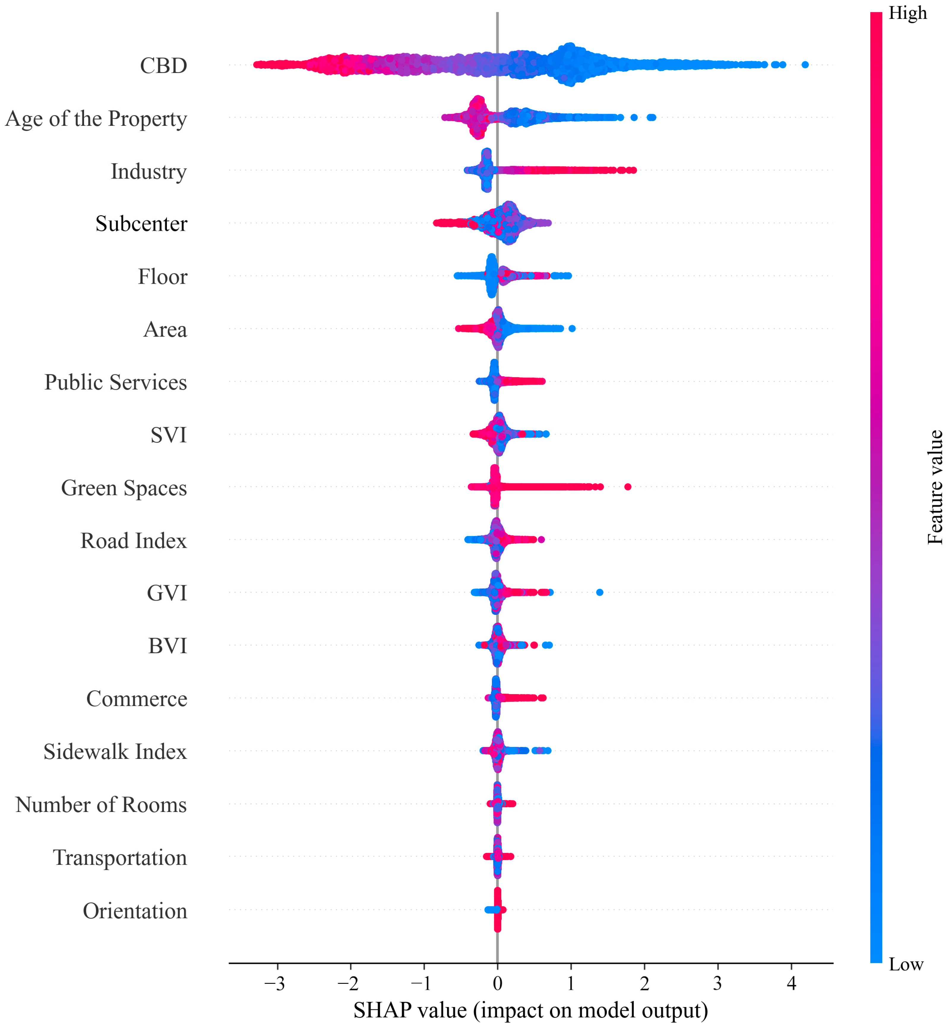
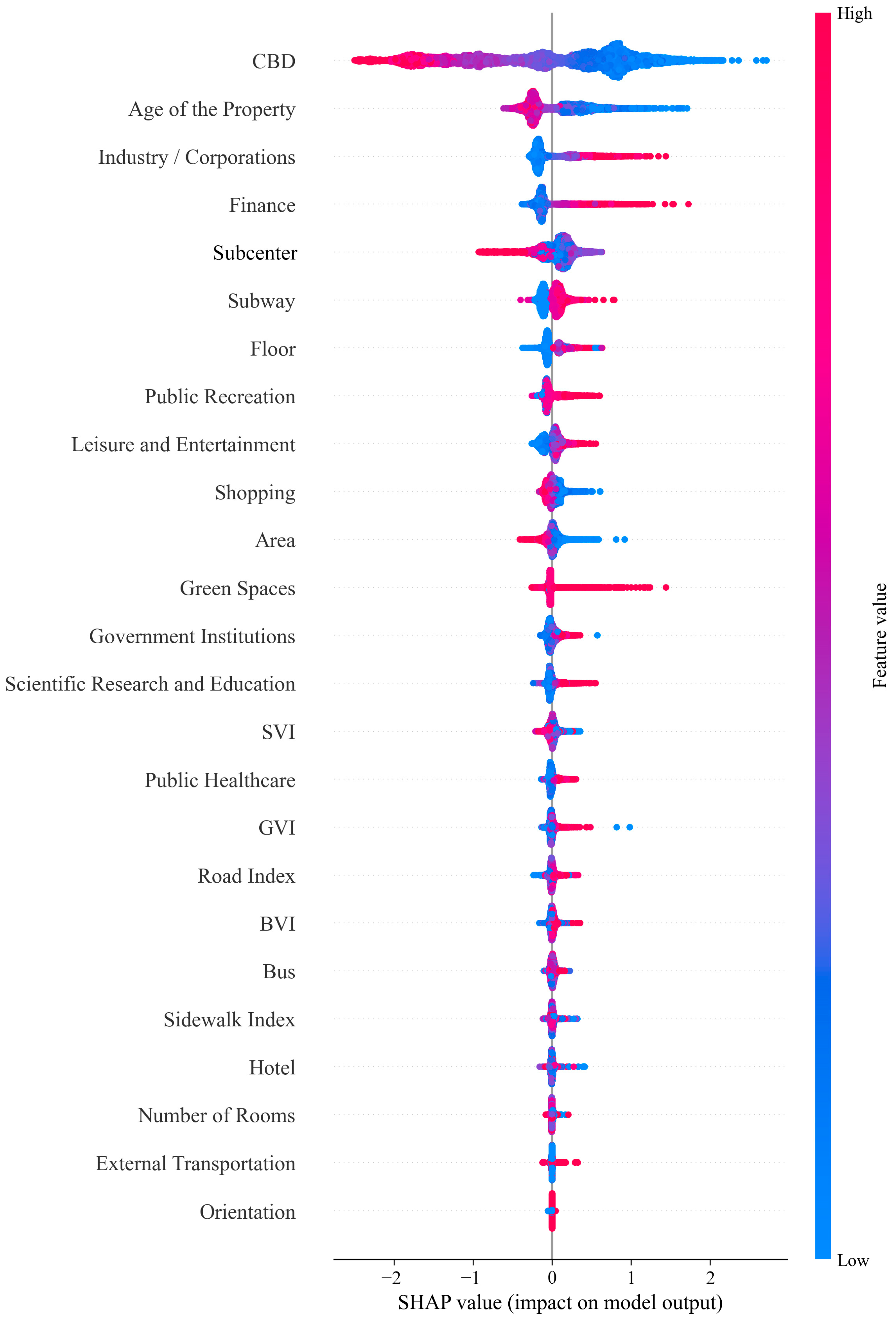
In this study, SHAP values are shown in Figure 6 and Figure 7 to quantify the impact of each factor. The Y axis represents the influencing factors, and they are sorted from top to bottom based on their importance. The X axis represents the SHAP value. Each point in the diagram refers to a sample of housing prices, and the color corresponds to the value of the factor.
As shown in Table 10, at the coarse-grained level, the RF model achieved an R2 of 0.8236, with an RMSE of 0.8243 and an MAE of 0.5334. The performance was further enhanced at the fine-grained level, with R2 increasing to 0.8389, while RMSE and MAE decreased to 0.7887 and 0.5014, respectively. In terms of accuracy, RF represented better performance than the regression model. From Figure 5, the coarse-grain POI shows a positive correlation with the housing price as a whole. At the fine-grained level, the housing prices were found to have different levels of dependence on the subclasses of POI. For example, at the coarse-grained level, the importance of transportation is at a low level. However, at the fine-grained level, the subway has a stronger contribution to housing prices. The contribution of public transportation and external traffic is relatively small. In the coarse-grained model, commercial facilities are positively correlated with housing prices. The RF model at the fine-grained level has better performance. Therefore, subsequent analysis will be carried out based on the fine-grained model.
In terms of the importance ranking of factors, the visual environment factors ranked low among the three built environment factors. The locational and neighborhood features have a greater contribution to the housing prices and are also the main determinants of the housing price in Shanghai. The importance rankings of the five visual environment factors are shown as follows: SVI, GVI, road index, BVI, and sidewalk index. In addition, from Figure 7, the relationship between visual environmental factors and housing prices is not obviously linear but more likely a complex and nonlinear relationship.
The comparative analysis of variable importance rankings further validates the advantages of RF in capturing the complex mechanisms of housing prices. From Table 11, proximity to the CBD consistently ranks first across both models and granularity levels, confirming its dominant role in determining housing prices in Shanghai. Although the importance of accessibility to subcenter decreases slightly in the RF model (ranking 4th and 5th in coarse- and fine-grained) compared to the hedonic model (2nd), it remains a significant factor. More notably, the RF model uncovers strong nonlinear relationships that the hedonic model fails to capture. Industry/Corporations ranked 15th in the hedonic model and rose to 3rd in RF. Shopping facility accessibility drops from 4th to 10th in importance, and hotel accessibility experiences a more pronounced decline from 8th to 22nd. These changes indicate that RF can provide a more detailed understanding of the complex and nonlinear driving factors of housing prices.

6.4. Nonlinear Relationship Analysis

To further explain the nonlinear relationship between various factors and housing prices, the variation of the SHAP value of some factors is shown in Figure 8. From Figure 8, the relationship between the distance to the CBD and the SHAP value can be approximately considered as linear. As the distance from the CBD increases, the SHAP value shows a monotonic decreasing trend. It is worth noting that when the distance from the housing to the CBD is less than 10 km, the SHAP values for most points are positive. The SHAP values of the subcenter showed an increasing and decreasing tendency, and the inflection points were approximately 14 km. Most of the SHAP values were positive when the subcenter was less than 14 km. When the subcenter exceeded 14 km, the SHAP value increased as the subcenter increased. The relationships between the values of the finance and SHAP value showed a similar pattern to the corporate enterprises. When the density of financial institutions or corporate enterprises around a housing area is below a certain threshold, both factors have a negative impact on housing prices. However, when the feature value exceeds this threshold, both factors present a positive correlation with the housing prices. This might be because the financial institutions in Shanghai are mainly concentrated within the inner ring road. The superior geographical location of this area is bound to lead to an increase in housing prices. The SHAP values of the shopping factor showed a trend of first stabilizing and then increasing. When the distance is less than 0.5 km, the shopping facilities remain negative. As the distance increases, the impact of SHAP on house prices continues to rise. For the subway factor, the SHAP values generally increased and then decreased as the feature value increased. Most points have positive SHAP values. This indicates that subway stations have a significant positive impact on housing prices in Shanghai.
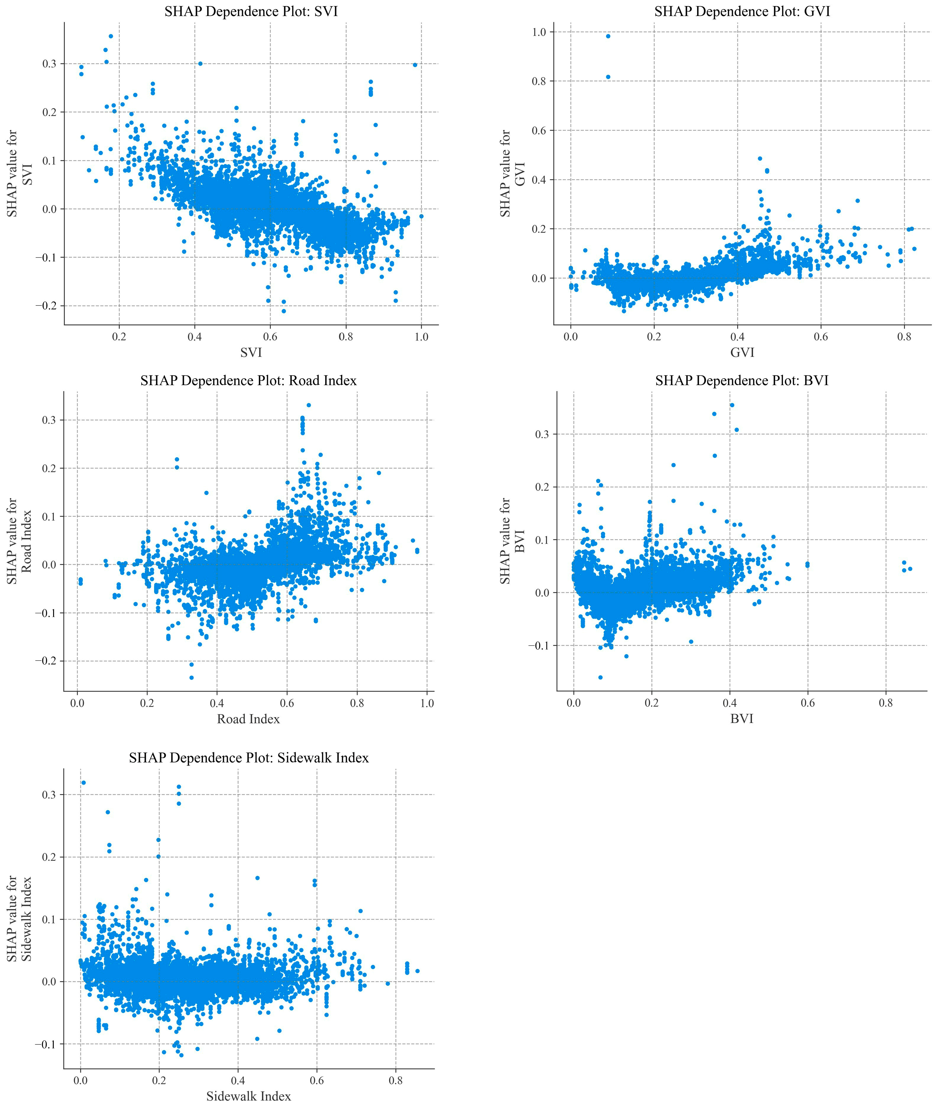
The variation of the SHAP value of 5 visual environmental factors is shown in Figure 9. The SVI reflects the openness of the view around the housing and also indirectly indicates the height and density of nearby buildings. For SVI values under 0.5, the SHAP values for most points are positive. As the SVI increases, its impact on housing prices gradually decreases. The result of the traditional hedonic model showed that the SVI had a significant negative effect on housing prices. It is indicated that the impact of SVI on housing prices is nonlinear. This is because the high housing prices in Shanghai have led to a compact urban landscape, with residents mostly in dense and high-rise apartments. The high-rise buildings mean enjoyment of air pollution in the higher floors [17]. The SHAP values of the GVI showed a stable trend and then increased. When the GVI is lower than 0.4, the GVI SHAP value remains stable at around zero. When the GVI exceeds 0.4, the SHAP values increase as the GVI increases. Based on the results of the hedonic pricing model, GVI has a nearly positive impact on housing prices. A study in Beijing also proved that GVI can cause housing prices to increase by 0.299% [75]. The relationship between the BVI and SHAP values also exhibits nonlinear characteristics. When the BVI is less than 0.1, it shows a negative correlation with housing prices. As the BVI increases, housing prices tend to decrease accordingly. The SHAP dependence plot for the road index shows that when the road index is less than 0.5, the SHAP values of most points are negative. Meanwhile, SHAP values exhibit an increasing trend above that threshold, with most points having positive SHAP values. This indicates that the proportion of visible road area has a positive impact on housing prices. The sidewalk index reflects the walkability of the neighborhood’s streets. In this study, the SHAP values for the sidewalk index fluctuate around 0, ranging between −0.1 and 0.1. This suggests that the sidewalk index does not have a clear or significant impact on housing prices.

7. Discussion

7.1. Results Discussion

Our research has constructed a new framework to reveal the influencing factors of housing prices. Many studies only use pre-specified forms of hedonic price models to quantify the relationship between housing prices and housing characteristics [46,76]. We compared the semi-log hedonic price model with RF. Our results showed that RF had a higher predictive ability, aligning with Tomasz Potrawa [77] that machine learning better captures the nonlinear relationships between housing prices and their determinants. Crucially, recognizing limitations in traditional approaches relying on coarse-grained POI classifications, we introduced a fine-grained POI framework. Unlike previous studies [17,78,79], we compared model performance at both fine-grained and coarse-grained levels. Fine-grained analysis has been proven to be more enlightening than coarse-grained POI, indicating that the accessibility of different facility types (such as hotel, finance, and shopping) has significantly different impacts on real estate value. These effects are masked within coarse-grained POI (such as commerce). This highlights the necessity of disaggregated data to accurately reveal the value drivers within the built environment.
Our research findings have clarified the specific mechanisms between the characteristics of the built environment and the housing market in Shanghai. Locational features, particularly proximity to the CBD within Shanghai’s concentric urban structure, emerged as the paramount pricing factor [49,80]. The accessibility of jobs, schools, healthcare, and other public services plays a key role in defining the housing price. While visual environmental features generally exhibited smaller effects, the significant positive impact of GVI strongly confirms the close connection between urban greening and property premium [17]. An interesting finding is that through SHAP analysis, it was shown that the accessibility of the subway has a nonlinear, inverted U-shaped relationship with the price, with the peak value approximately at 0.5 km. This is because homebuyers would not like there to be too many subway stations near their living areas [78]. This optimal distance balances accessibility benefits against noise hazards, offering practical guidance for buyers and planners. The sidewalk index showed no significant impact on housing prices. The reason for this result might be that the sidewalks are blocked by other elements during the semantic segmentation of street view images. It suggests methodological considerations for future visual environment studies.

7.2. Limitations and Potential Improvements

There are still some shortcomings in this research, which can be improved in future work:
This study only selects Shanghai as the research area. Due to the differences in built environments across cities, the results of this study may vary when applied to other cities. Future research could consider conducting empirical analyses in cities such as Beijing and Shenzhen. The feasibility of the framework is further verified by changing the size of the buffer zone and the number of RF trees according to the specific local conditions.
This study acknowledges potential endogeneity due to household self-selection in residential locations. Unobserved neighborhood characteristics may correlate with key predictors such as distance to CBD or GVI. High-income households may prefer homes near the CBD due to unobserved advantages like school quality and social prestige, possibly underestimating the negative correlation between housing prices and distance from the CBD. In the future, we will supplement the omitted variables into the model to control the endogeneity problem to the greatest extent. In the future, questionnaire data will be incorporated to obtain the variables such as residents’ subjective perceptions and motivations for their housing choices. Furthermore, we will actively seek an effective instrumental variable and use spatial econometric models to more rigorously identify the impact of the built environment on housing prices.
This study overlooked the analysis of spatial heterogeneity and spatial dependence, which could potentially bias our findings, especially concerning key variables such as “distance to CBD”. According to previous studies [80], the distance to the CBD is indeed the most important factor. In our future research, more in-depth insights will be provided, and potential biases will be reduced through spatial econometric models or the Geographically Weighted Regression (GWR) method.
The spatial weight matrices used in this experiment were all spatial adjacency matrices, and no economic distance matrices or technical correlation matrices were employed. In future experiments, we will further utilize nighttime light remote sensing data to construct matrices such as economic distance matrices for spatial analysis.

7.3. Implications for Urban Planning

This study explores macro- and micro-level effects of the built environment on Shanghai housing prices, offering practical guidance for urban planning. The housing prices in the areas close to the CBD in Shanghai are particularly high, which contradicts the multi-center development goals of the local authorities. To decentralize housing demand from the core CBD and promote polycentric development, it is essential to enhance public transportation connectivity. Priority should be given to expanding metro services in emerging subcenters and the five new towns: Jiading, Songjiang, Qingpu, Fengxian, and Nanhui. Moreover, it is suggested to integrate financial, industrial, and commercial facilities in a balanced manner. Furthermore, this study highlights the impact of the visual environment on housing prices, indicating that urban planning efforts should not neglect the aesthetic and visual quality of the community. Attention should be paid to the micro-street environment around the residence. For instance, developers can enhance property value and appeal to potential buyers by incorporating elements like green spaces and visually pleasing surroundings within or near residential areas.

8. Conclusions

This study constructs an explanatory framework for factors influencing housing prices based on street view images, housing price data, and POI data. The hedonic price model and RF used in this study reveal complex nonlinear effects of various factors on housing prices. The RF achieves a higher accuracy rate than the hedonic price model. Specifically, at the coarse-grained level, the R2 value of the price model is 0.7680; at the fine-grained level, it is 0.7918; and the corresponding R2 values of the RF model are 0.8236 and 0.8389, respectively. The accessibility of locations and the accessibility of various functions (such as industry/corporations, subway, and finance) have a significant impact on property prices. The contribution of visual environmental factors to housing prices is relatively small. Compared with the coarse-grained POIs, fine-grained POIs can reflect the dependence of housing prices on various functional POIs better and are more suitable for investigating the influencing mechanisms of housing prices. Its influence is nuanced by accessibility in different dimensions. In the hedonic price model regression results, the influence of the commerce factor on house prices is very low. In contrast, shopping and hotels have a higher impact on housing prices at the fine-grained POI. Similar results are also observed in the RF. Our results further investigate the factors that affect housing prices across large areas, providing valuable insights for urban planners.

Author Contributions

Conceptualization, Ziyi Wang and Yu Wang; methodology, Yu Wang; software, Yu Wang and Shaozhu Chen; validation, Xinyu Xia; investigation, Xinyu Xia and Shaozhu Chen; writing—original draft preparation, Wei Jiang and Ziyi Wang; writing—review and editing, Wei Jiang, Xinyu Xia and Ziyi Wang; supervision, Wei Jiang and Yu Wang. All authors have read and agreed to the published version of the manuscript.

Funding

This research was funded by the National Natural Science Foundation of China (Grant 42301490) and the Undergraduate Innovation and Entrepreneurship Training Program of Anhui Normal University (Grant S202410370039).

Data Availability Statement

The data in this study are openly available. The housing prices were acquired from Lianjia (https://sn.lianjia.com/, accessed on 31 October 2025); the POI data were obtained from the API of Gaode, available at https://lbs.amap.com/, accessed on 31 October 2025; and the street view images data were collected from the Baidu Maps Open Platform (https://lbsyun.baidu.com/, accessed on 31 October 2025). Further inquiries can be directed to the corresponding author.

Conflicts of Interest

The authors declare no conflicts of interest.

Appendix A

Table A1. The results of key variables under different radius buffer zones in the hedonic pricing model.
Factors (Coarse-Grained)800-m Buffer Zone1000-m Buffer Zone1200-m Buffer ZoneFactors (Fine-Grained)800-m Buffer Zone1000-m Buffer Zone1200-m Buffer Zone
CBD−1.0032 ***−0.9249 ***−0.9985 ***CBD−0.9642 ***−0.8895 ***−0.9770 ***
Subcenter0.2794 ***0.2396 ***0.2765 ***Subcenter0.2675 ***0.2411 ***0.2879 ***
Commerce0.0398 ***0.0320 ***0.0374 ***Finance0.0014 ***0.0092 ***0.0061 ***
Public Services0.0291 ***0.0997 ***0.0457 ***Subway0.0811 ***0.1016 ***0.0678 ***
Model
performance
R20.75130.76800.7526R20.76110.79180.7591
RMSE0.17530.16930.1748RMSE0.17180.16040.1725
MAE0.13470.12870.1342MAE0.13090.12080.1318
Note: Significance: *** p < 0.001.

References

  1. Liangjin, Z.; Enjun, X. Research Review on Infliencing Factor of House Price Abroad. J. Technol. Econ. 2018, 37, 111–119. [Google Scholar]
  2. Chen, M.; Liu, Y.; Arribas-Bel, D.; Singleton, A. Assessing the value of user-generated images of urban surroundings for house price estimation. Landsc. Urban Plan. 2022, 226, 104486. [Google Scholar] [CrossRef]
  3. Bailey, J.R.; Lindquist, W.B.; Rachev, S.T. Hedonic Models Incorporating Environmental, Social, and Governance Factors for Time Series of Average Annual Home Prices. J. Risk Financ. Manag. 2024, 17, 375. [Google Scholar] [CrossRef]
  4. Xu, X.; Qiu, W.; Li, W.; Liu, X.; Zhang, Z.; Li, X.; Luo, D. Associations between Street-View Perceptions and Housing Prices: Subjective vs. Objective Measures Using Computer Vision and Machine Learning Techniques. Remote Sens. 2022, 14, 891. [Google Scholar] [CrossRef]
  5. Li, H.; Chen, P.; Grant, R. Built environment, special economic zone, and housing prices in Shenzhen, China. Applied Geography 2021, 129, 102429. [Google Scholar] [CrossRef]
  6. Kaklauskas, A.; Gudauskas, R. 17—Intelligent decision-support systems and the Internet of Things for the smart built environment. In Start-Up Creation; Pacheco-Torgal, F., Rasmussen, E., Granqvist, C.-G., Ivanov, V., Kaklauskas, A., Makonin, S., Eds.; Woodhead Publishing: Cambridge, UK, 2016; pp. 413–449. [Google Scholar] [CrossRef]
  7. Xiao, Y. Urban Morphology and Housing Market; Springer: Berlin/Heidelberg, Germany, 2017. [Google Scholar] [CrossRef]
  8. Yang, L.; Wang, B.; Zhou, J.; Wang, X. Walking accessibility and property prices. Transp. Res. Part D Transp. Environ. 2018, 62, 551–562. [Google Scholar] [CrossRef]
  9. Gu, Z.; Tang, M.; Luo, X.; Feng, J. Examination of the impacts of hospital accessibility on housing prices: Heterogeneity across attributes, space and price quantiles. J. Hous. Built Environ. 2023, 39, 179–200. [Google Scholar] [CrossRef]
  10. Wen, H.; Xiao, Y.; Hui, E.C.M. Quantile effect of educational facilities on housing price: Do homebuyers of higher-priced housing pay more for educational resources? Cities 2019, 90, 100–112. [Google Scholar] [CrossRef]
  11. Chen, K.; Lin, H.; Cao, F.; Han, Y.; You, S.; Shyr, O.; Lu, Y.; Huang, X. Do hospital and rail accessibility have a consistent influence on housing prices? Empirical evidence from China. Front. Environ. Sci. 2022, 10, 1044600. [Google Scholar] [CrossRef]
  12. Chiesura, A. The role of urban parks for the sustainable city. Landsc. Urban Plan. 2004, 68, 129–138. [Google Scholar] [CrossRef]
  13. Jim, C.Y.; Chen, W.Y. Impacts of urban environmental elements on residential housing prices in Guangzhou (China). Landsc. Urban Plan. 2006, 78, 422–434. [Google Scholar] [CrossRef]
  14. van den Berg, M.; van Poppel, M.; van Kamp, I.; Andrusaityte, S.; Balseviciene, B.; Cirach, M.; Danileviciute, A.; Ellis, N.; Hurst, G.; Masterson, D.; et al. Visiting green space is associated with mental health and vitality: A cross-sectional study in four european cities. Health Place 2016, 38, 8–15. [Google Scholar] [CrossRef]
  15. Gubbels, J.S.; Kremers, S.P.J.; Droomers, M.; Hoefnagels, C.; Stronks, K.; Hosman, C.; de Vries, S. The impact of greenery on physical activity and mental health of adolescent and adult residents of deprived neighborhoods: A longitudinal study. Health Place 2016, 40, 153–160. [Google Scholar] [CrossRef] [PubMed]
  16. Fu, X.; Jia, T.; Zhang, X.; Li, S.; Zhang, Y. Do street-level scene perceptions affect housing prices in Chinese megacities? An analysis using open access datasets and deep learning. PLoS ONE 2019, 14, e0217505. [Google Scholar] [CrossRef] [PubMed]
  17. Chen, L.; Yao, X.; Liu, Y.; Zhu, Y.; Chen, W.; Zhao, X.; Chi, T. Measuring Impacts of Urban Environmental Elements on Housing Prices Based on Multisource Data—A Case Study of Shanghai, China. ISPRS Int. J. Geo Inf. 2020, 9, 106. [Google Scholar] [CrossRef]
  18. Fan, Z.; Yu, L. Street view imagery: Methods and applications based on artificial intelligence. Natl. Remote Sens. Bull. 2021, 25, 1043–1054. [Google Scholar] [CrossRef]
  19. Lee, C.L. An examination of the risk-return relation in the Australian housing market. Int. J. Hous. Mark. Anal. 2017, 10, 431–449. [Google Scholar] [CrossRef]
  20. Al-Masum, M.A.; Lee, C.L. Modelling housing prices and market fundamentals: Evidence from the Sydney housing market. Int. J. Hous. Mark. Anal. 2020, 12, 746–762. [Google Scholar] [CrossRef]
  21. Trojanek, R.; Gluszak, M. Spatial and time effect of subway on property prices. J. Hous. Built Environ. 2018, 33, 359–384. [Google Scholar] [CrossRef]
  22. Yamagata, Y.; Murakami, D.; Yoshida, T.; Seya, H.; Kuroda, S. Value of urban views in a bay city: Hedonic analysis with the spatial multilevel additive regression (SMAR) model. Landsc. Urban Plan. 2016, 151, 89–102. [Google Scholar] [CrossRef]
  23. Malpezzi, S. Hedonic Pricing Models: A Selective and Applied Review. Hous. Econ. Public Policy 2002, 1, 67–89. [Google Scholar] [CrossRef]
  24. Rosen, S. Hedonic Prices and Implicit Markets: Product Differentiation in Pure Competition. J. Political Econ. 1974, 82, 34–55. [Google Scholar] [CrossRef]
  25. Efthymiou, D.; Antoniou, C. How do transport infrastructure and policies affect house prices and rents? Evidence from Athens, Greece. Transp. Res. Part A Policy Pract. 2013, 52, 1–22. [Google Scholar] [CrossRef]
  26. Huang, H.; Yin, L. Creating sustainable urban built environments: An application of hedonic house price models in Wuhan, China. J. Hous. Built Environ. 2015, 30, 219–235. [Google Scholar] [CrossRef]
  27. Bolitzer, B.; Netusil, N.R. The impact of open spaces on property values in Portland, Oregon. J. Environ. Manag. 2000, 59, 185–193. [Google Scholar] [CrossRef]
  28. Glaeser, E.L.; Kominers, S.D.; Luca, M.; Naik, N. Big Data and Big Cities: The Promises and Limitations of Improved Measures of Urban Life. Econ. Inq. 2018, 56, 114–137. [Google Scholar] [CrossRef]
  29. Li, H. Institutions, Economic Transition and Urban Land Expansion in China. Ph.D. Thesis, Universiteit Utrecht, Utrecht, The Netherlands, 2016. [Google Scholar] [CrossRef]
  30. Han, R.; Wu, S.; He, F.; Sun, Q. Natural Attraction and Driving Forces: Analyzing the Impact of Parkland on Residential Prices and Typological Difference*. J. Sustain. For. 2025, 44, 50–70. [Google Scholar] [CrossRef]
  31. Hu, L.; He, S. How does the second-hand housing price regulatory policy differentiate the housing price premiums for multi-dimensional school qualities? Evidence from a quasi-natural experiment in urban China. Int. J. Hous. Policy 2024, 1–22. [Google Scholar] [CrossRef]
  32. Wen, H.; Zhang, Y.; Zhang, L. Do educational facilities affect housing price? An empirical study in Hangzhou, China. Habitat Int. 2014, 42, 155–163. [Google Scholar] [CrossRef]
  33. Yi, W.; Ruiping, R.; Deng, G. Neighborhood Quality and Housing Value: Evidence from Urban Micro Data. J. Manag. Sustain. 2024, 2, 128. [Google Scholar] [CrossRef]
  34. Fletcher, M.; Gallimore, P.; Mangan, J. Heteroscedasticity in hedonic house price models. J. Prop. Res. 2000, 17, 93–108. [Google Scholar] [CrossRef]
  35. Linneman, P. Some empirical results on the nature of the hedonic price function for the urban housing market. J. Urban Econ. 1980, 8, 47–68. [Google Scholar] [CrossRef]
  36. Carroll, T.M.; Clauretie, T.M.; Jensen, J. Living next to godliness: Residential property values and churches. J. Real Estate Financ. Econ. 1996, 12, 319–330. [Google Scholar] [CrossRef]
  37. Dai, J.; Lv, P.; Ma, Z.; Bi, J.; Wen, T. Environmental risk and housing price: An empirical study of Nanjing, China. J. Clean. Prod. 2020, 252, 119828. [Google Scholar] [CrossRef]
  38. Strohbach, M.W.; Arnold, E.; Haase, D. The carbon footprint of urban green space—A life cycle approach. Landsc. Urban Plan. 2012, 104, 220–229. [Google Scholar] [CrossRef]
  39. Haaland, C.; van den Bosch, C.K. Challenges and strategies for urban green-space planning in cities undergoing densification: A review. Urban For. Urban Green. 2015, 14, 760–771. [Google Scholar] [CrossRef]
  40. Belcher, R.N.; Chisholm, R.A. Tropical Vegetation and Residential Property Value: A Hedonic Pricing Analysis in Singapore. Ecol. Econ. 2018, 149, 149–159. [Google Scholar] [CrossRef]
  41. Donovan, G.H.; Butry, D.T. The effect of urban trees on the rental price of single-family homes in Portland, Oregon. Urban For. Urban Green. 2011, 10, 163–168. [Google Scholar] [CrossRef]
  42. Asgarzadeh, M.; Koga, T.; Hirate, K.; Farvid, M.; Lusk, A. Investigating oppressiveness and spaciousness in relation to building, trees, sky and ground surface: A study in Tokyo. Landsc. Urban Plan. 2014, 131, 36–41. [Google Scholar] [CrossRef]
  43. Nutsford, D.; Pearson, A.L.; Kingham, S.; Reitsma, F. Residential exposure to visible blue space (but not green space) associated with lower psychological distress in a capital city. Health Place 2016, 39, 70–78. [Google Scholar] [CrossRef]
  44. Luttik, J. The value of trees, water and open space as reflected by house prices in the Netherlands. Landsc. Urban Plan. 2000, 48, 161–167. [Google Scholar] [CrossRef]
  45. Jim, C.Y.; Chen, W.Y. Value of scenic views: Hedonic assessment of private housing in Hong Kong. Landsc. Urban Plan. 2009, 91, 226–234. [Google Scholar] [CrossRef]
  46. Karato, K.; Movshuk, O.; Shimizu, C. Semiparametric Model of Hedonic Housing Prices in Japan. Asian Econ. J. 2015, 29, 325–345. [Google Scholar] [CrossRef]
  47. Lancaster, K.J.J.J.o.p.e. A new approach to consumer theory. J. Political Econ. 1966, 74, 132–157. [Google Scholar] [CrossRef]
  48. Sakia, R. The Box-Cox Transformation Technique: A Review. J. R. Stat. Soc. Ser. D Stat. 1992, 41, 169–178. [Google Scholar] [CrossRef]
  49. Tam, V.W.Y.; Fung, I.W.H.; Wang, J.; Ma, M. Effects of locations, structures and neighbourhoods to housing price: An empirical study in Shanghai, China. Int. J. Constr. Manag. 2022, 22, 1288–1307. [Google Scholar] [CrossRef]
  50. Yu, P.; Changcheng, K.; Anrong, D. Street Greenspace Justice Assessment Study of Dongcheng District in Beijing Based on Street View Data. Chin. Landsc. Archit. 2020, 36, 51–56. [Google Scholar] [CrossRef]
  51. Naik, N.; Kominers, S.D.; Raskar, R.; Glaeser, E.L.; Hidalgo, C.A. Computer vision uncovers predictors of physical urban change. Proc. Natl. Acad. Sci. USA 2017, 114, 7571–7576. [Google Scholar] [CrossRef] [PubMed]
  52. Chen, L.-C.; Zhu, Y.; Papandreou, G.; Schroff, F.; Adam, H. Encoder-decoder with atrous separable convolution for semantic image segmentation. In Proceedings of the European Conference on Computer Vision (ECCV), Munich, Germany, 8–14 September 2018; pp. 801–818. [Google Scholar] [CrossRef]
  53. Song, L.; Liu, D.; Kwan, M.-P.; Liu, Y.; Zhang, Y. Machine-based understanding of noise perception in urban environments using mobility-based sensing data. Comput. Environ. Urban Syst. 2024, 114, 102204. [Google Scholar] [CrossRef]
  54. Zhou, B.; Lapedriza, A.; Khosla, A.; Oliva, A.; Torralba, A. Places: A 10 Million Image Database for Scene Recognition. IEEE Trans. Pattern Anal. Mach. Intell. 2018, 40, 1452–1464. [Google Scholar] [CrossRef] [PubMed]
  55. Zhang, F.; Zhou, B.; Liu, L.; Liu, Y.; Fung, H.H.; Lin, H.; Ratti, C. Measuring human perceptions of a large-scale urban region using machine learning. Landsc. Urban Plan. 2018, 180, 148–160. [Google Scholar] [CrossRef]
  56. Ramírez, T.; Hurtubia, R.; Lobel, H.; Rossetti, T. Measuring heterogeneous perception of urban space with massive data and machine learning: An application to safety. Landsc. Urban Plan. 2021, 208, 104002. [Google Scholar] [CrossRef]
  57. Yin, L.; Wang, Z. Measuring visual enclosure for street walkability: Using machine learning algorithms and Google Street View imagery. Appl. Geogr. 2016, 76, 147–153. [Google Scholar] [CrossRef]
  58. Wang, L.; Hou, C.; Zhang, Y.; He, J. Measuring solar radiation and spatio-temporal distribution in different street network direction through solar trajectories and street view images. Int. J. Appl. Earth Obs. Geoinf. 2024, 132, 104058. [Google Scholar] [CrossRef]
  59. Jiang, S.; Alves, A.; Rodrigues, F.; Ferreira, J.; Pereira, F.C. Mining point-of-interest data from social networks for urban land use classification and disaggregation. Comput. Environ. Urban Syst. 2015, 53, 36–46. [Google Scholar] [CrossRef]
  60. Zhang, Z.; Zhao, X.; Wang, G.; Bi, X. A New Point-of-Interest Classification Model with an Extreme Learning Machine. Cogn. Comput. 2018, 10, 951–964. [Google Scholar] [CrossRef]
  61. Li, H.; Miao, L. A Study of the Non-Linear Relationship Between Urban Morphology and Vitality in Heritage Areas Based on Multi-Source Data and Machine Learning: A Case Study of Dalian. ISPRS Int. J. Geo Inf. 2025, 14, 177. [Google Scholar] [CrossRef]
  62. Xu, J.; Liu, Y.; Liu, Y.; An, R.; Tong, Z. Integrating street view images and deep learning to explore the association between human perceptions of the built environment and cardiovascular disease in older adults. Soc. Sci. Med. 2023, 338, 116304. [Google Scholar] [CrossRef]
  63. Sirmans, G.S.; Macpherson, D.A.; Zietz, E.N. The Composition of Hedonic Pricing Models. J. Real Estate Lit. 2005, 13, 3–43. [Google Scholar] [CrossRef]
  64. Hu, L.; He, S.; Han, Z.; Xiao, H.; Su, S.; Weng, M.; Cai, Z. Monitoring housing rental prices based on social media: An integrated approach of machine-learning algorithms and hedonic modeling to inform equitable housing policies. Land Use Policy 2019, 82, 657–673. [Google Scholar] [CrossRef]
  65. Li, H.; Wei, Y.D.; Wu, Y.; Tian, G. Analyzing housing prices in Shanghai with open data: Amenity, accessibility and urban structure. Cities 2019, 91, 165–179. [Google Scholar] [CrossRef]
  66. Dou, M.; Gu, Y.; Fan, H. Incorporating neighborhoods with explainable artificial intelligence for modeling fine-scale housing prices. Appl. Geogr. 2023, 158, 103032. [Google Scholar] [CrossRef]
  67. Chollet, F. Xception: Deep Learning with Depthwise Separable Convolutions. In Proceedings of the 2017 IEEE Conference on Computer Vision and Pattern Recognition (CVPR), Honolulu, HI, USA, 21–26 July 2017; pp. 1800–1807. [Google Scholar] [CrossRef]
  68. Lundberg, S.M.; Lee, S.-I. A unified approach to interpreting model predictions. In Proceedings of the 31st International Conference on Neural Information Processing Systems, Long Beach, CA, USA, 4–9 December 2017; pp. 4768–4777. [Google Scholar] [CrossRef]
  69. Li, Z. Extracting spatial effects from machine learning model using local interpretation method: An example of SHAP and XGBoost. Comput. Environ. Urban Syst. 2022, 96, 101845. [Google Scholar] [CrossRef]
  70. Salih, A.M.; Raisi-Estabragh, Z.; Galazzo, I.B.; Radeva, P.; Petersen, S.E.; Lekadir, K.; Menegaz, G. A Perspective on Explainable Artificial Intelligence Methods: SHAP and LIME. Adv. Intell. Syst. 2025, 7, 2400304. [Google Scholar] [CrossRef]
  71. Lipovetsky, S.; Conklin, M. Analysis of regression in game theory approach. Appl. Stoch. Models Bus. Ind. 2001, 17, 319–330. [Google Scholar] [CrossRef]
  72. Ribeiro, M.; Singh, S.; Guestrin, C. “Why Should I Trust You?”: Explaining the Predictions of Any Classifier; Association for Computational Linguistics: Stroudsburg, PA, USA, 2016; pp. 1135–1144. [Google Scholar] [CrossRef]
  73. Štrumbelj, E.; Kononenko, I. Explaining prediction models and individual predictions with feature contributions. Knowl. Inf. Syst. 2014, 41, 647–665. [Google Scholar] [CrossRef]
  74. Datta, A.; Sen, S.; Zick, Y. Algorithmic Transparency via Quantitative Input Influence: Theory and Experiments with Learning Systems. In Proceedings of the 2016 IEEE Symposium on Security and Privacy (SP), San Jose, CA, USA, 22–26 May 2016; pp. 598–617. [Google Scholar] [CrossRef]
  75. Liao, X.; Deng, M.; Huang, H. Analyzing Multiscale Spatial Relationships between the House Price and Visual Environment Factors. Appl. Sci. 2021, 12, 213. [Google Scholar] [CrossRef]
  76. Luo, H.; Zhao, S.; Yao, R. Determinants of Housing Prices in Dalian City, China: Empirical Study Based on Hedonic Price Model. J. Urban Plan. Dev. 2021, 147, 05021017. [Google Scholar] [CrossRef]
  77. Potrawa, T.; Tetereva, A. How much is the view from the window worth? Machine learning-driven hedonic pricing model of the real estate market. J. Bus. Res. 2022, 144, 50–65. [Google Scholar] [CrossRef]
  78. Zhang, Y.; Dong, R. Impacts of Street-Visible Greenery on Housing Prices: Evidence from a Hedonic Price Model and a Massive Street View Image Dataset in Beijing. ISPRS Int. J. Geo Inf. 2018, 7, 104. [Google Scholar] [CrossRef]
  79. Zhu, J.; Gong, Y.; Liu, C.; Du, J.; Song, C.; Chen, J.; Pei, T. Assessing the Effects of Subjective and Objective Measures on Housing Prices with Street View Imagery: A Case Study of Suzhou. Land 2023, 12, 2095. [Google Scholar] [CrossRef]
  80. Chen, J.; Hao, Q. The impacts of distance to CBD on housing prices in Shanghai: A hedonic analysis. J. Chin. Econ. Bus. Stud. 2008, 6, 291–302. [Google Scholar] [CrossRef]
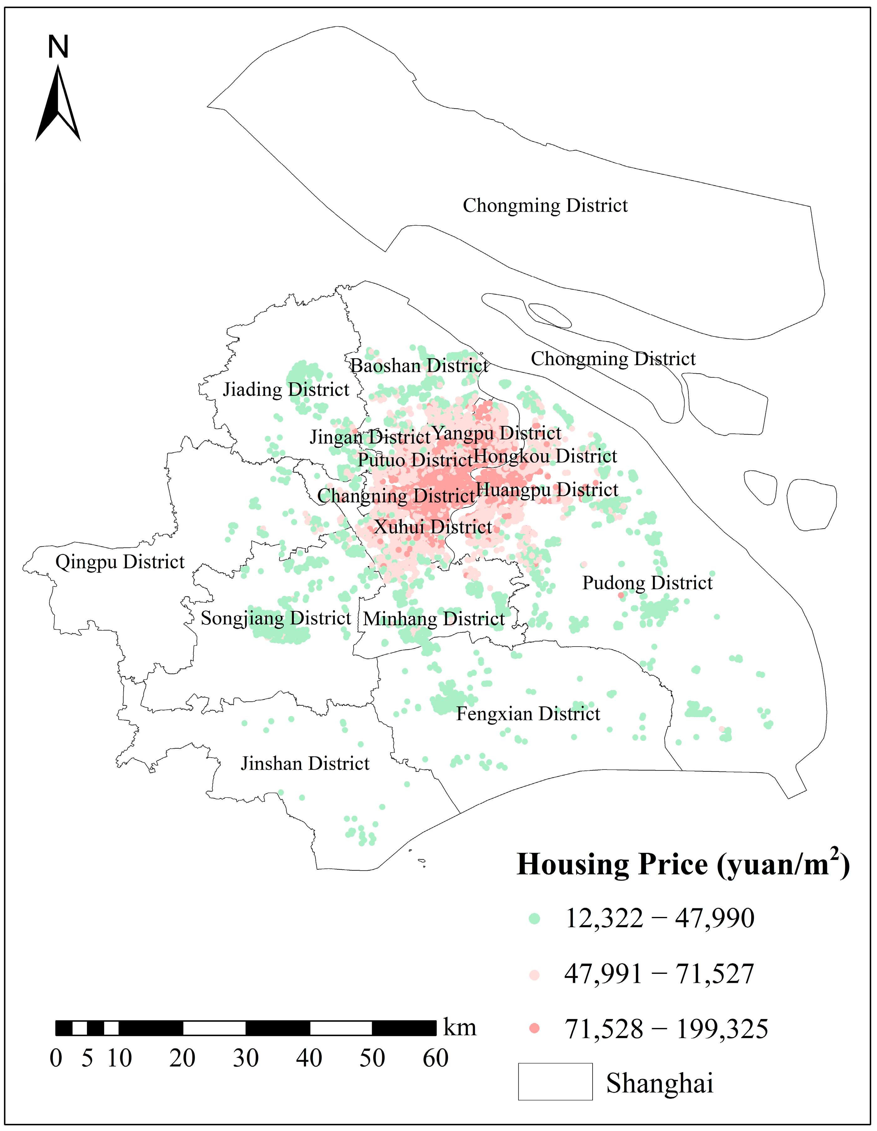
Figure 1. The spatial distribution of second-hand homes.
Ijgi 14 00436 g001
Figure 2. The spatial distribution of street view images in Shanghai.
Ijgi 14 00436 g002
Figure 3. Research framework diagram.
Ijgi 14 00436 g003
Figure 4. LISA clustering map.
Ijgi 14 00436 g004
Figure 5. Hotspot analysis of Shanghai housing prices.
Ijgi 14 00436 g005
Figure 6. Coarse-grained RF regression model SHAP summary plot.
Ijgi 14 00436 g006
Figure 7. Fine-grained RF regression model SHAP summary plot.
Ijgi 14 00436 g007
Figure 8. SHAP dependence plot for key built environment factors.
Ijgi 14 00436 g008aIjgi 14 00436 g008b
Figure 9. SHAP dependence plot for visual environment feature variables.
Ijgi 14 00436 g009
Table 1. Second-hand homes’ data details.
Field NameField AttributesExample
District and streetThe house’s district and streetTianshan Road Subdistrict, Changning District
Neighborhood nameThe name of neighborhoodXinfeng Community
Property typeThe type of propertyone room, one living room, one kitchen, one bathroom
Floor levelNumber of floors6
Building areaFloor area (m2)50.4
OrientationBinary value: 1 for south-facing and north-south-facing, 0 otherwise1
Listing priceThe second-hand home’s listed sale price (10,000 yuan/m2)5.72
Unit priceHousing unit price (10,000 yuan/m2)6.68
Table 2. POI data details table.
Field NameField AttributesExample
IDUnique Identifier for POIB0FFI6407I
NameName of POISuper Life Plaza (Xincun Branch)
XLongitude of POI31.266869
YLatitude of POI121.435744
DistrictAdministrative Region of POIPutuo District
TypePOI Type (Major Category; Intermediate Category; Minor Category)Shopping Services; Supermarket; Grocery Store
AddressSpecific Location of POI50 m north of the intersection of Yichuan Road and Xincun Road
Table 3. POI data classification.
Coarse-Grained POIFine-Grained POIGaode POI Subcategories
CommerceHotelHotels, Inns, and Guesthouses
ShoppingConvenience Store, Supermarket, Shopping Mall, Specialty Shopping Streets, Integrated Markets
FinanceBanks, ATMs, Securities Firms, Insurance Companies, Financial Companies, Financial and Insurance Service Institutions
Entertainment and LeisureLeisure Venues, Cinemas and Theaters, Entertainment Venues, Golf-related, Sports and Leisure Service Venues
TransportationExternal TransportationAirport, Train Station, Long-Distance Bus Station, Port Terminal, Ferry Station
Public TransportationBus Station
SubwaySubway Station
IndustryCompanies and EnterprisesIndustrial Parks, Companies, Agriculture, Forestry, Animal Husbandry, and Fishery Bases, Factories
Public ServicesPublic TourismMuseums, Libraries, Archives, Science Museums, Art Museums, Exhibition Halls, Planetariums
Research and EducationUniversities, High Schools, Primary Schools, Kindergartens, Vocational and Technical Schools, Research Institutions
Government AgenciesGovernment Agencies, Social Organizations, Public Security and Judicial Institutions, Foreign Organizations, Democratic Parties, Industry and Taxation Agencies, Traffic Vehicle Management
Public HealthcareGeneral Hospitals, Specialized Hospitals, Emergency Centers, Disease Prevention Institutions
Green SpacesGreen Spaces Parks, Zoos, Botanical Gardens, Aquariums, Urban Squares, Scenic Spots
Table 4. Descriptive statistics of housing characteristic variables.
VariableMeanStandard DeviationMinimum ValueMaximum ValueDescription
Dependent VariableHousing Price5.8272.041.14819.988Housing unit price (10,000 yuan/m2)
Structural FeaturesNumber of Rooms3.5941.311118Number of rooms
Area87.12343.805211042.17Floor area (m2)
Floor10.6247.547180Number of floors
Orientation0.8330.37301Binary value: 1 for south-facing and north-south-facing, 0 otherwise
Property Age19.1499.8141107Calculated as 2018 minus construction year
Locational FeaturesCBD13.3879.0470.3558.545Distance to People’s Square of Shanghai (km)
Subcenter14.3719.7170.3463.156Distance to the nearest subcenter(km)
Transportation0.4960.05000.8Average distance to transportation POIs within 1000 m (km)
External Transportation0.0980.14800.7Average distance to external transportation POIs within 1000 m
Subway0.2290.18300.7Average distance to subway station POIs within 1000 m (km)
Bus0.4220.05800.7Average distance to public bus station POIs within 1000 m (km)
Neighborhood FeaturesCommerce0.5100.07400.8Average distance to commerce POIs within 1000 m (km)
Hotel0.3480.04900.7Average distance to hotel POIs within 1000 m (km)
Shopping0.3970.06100.7Average distance to shopping POIs within 1000 m (km)
Finance0.3270.04600.7Average distance to finance POIs within 1000 m (km)
Leisure and Entertainment0.3880.06900.7Average distance to leisure and entertainment POIs within 1000 m (km)
Industry0.4790.0750.40.8Average distance to industry POIs within 1000 m (km)
Industry/Corporations0.3590.0670.30.8Average distance to industry/corporations POIs within 1000 m (km)
Public Services0.5150.09100.8Average distance to public services POIs within 1000 m (km)
Public Recreation0.2640.15400.7Average distance to public recreation POIs within 1000 m (km)
Scientific Research and Education0.3370.05300.7Average distance to scientific research and education POIs within 1000 m (km)
Public Healthcare0.3360.09100.7Average distance to public healthcare POIs within 1000 m (km)
Government Institutions0.3900.07900.7Average distance to government institutions POIs within 1000 m (km)
Green Spaces0.3140.09200.7Average distance to green spaces POIs within 1000 m (km)
Visual Environmental FeaturesGVI0.2050.0840.0010.75Average GVI within 400 m
SVI0.4660.1030.0180.75Average SVI within 400 m
BVI0.1250.0690.0010.729Average BVI within 400 m
Road Index0.0870.0150.0210.148Average road index within 400 m
Sidewalk Index0.0130.00600.049Average sidewalk index within 400 m
Note: Bold text represents coarse-grained feature variables.
Table 5. The values of hyperparameters.
HyperparameterCoarse-GrainedFine-GrainedDescription
n_estimators180180The number of decision trees in the ensemble
random_state4242A seed value to ensure reproducibility by controlling the stochasticity in forest generation
max_depth2249The maximum depth of each tree. Limiting the tree depth can help prevent overfitting
min_samples_leaf11The minimum number of samples required to be at a leaf node. This parameter can also help control overfitting
min_samples_split22The minimum number of samples for node splitting. Increasing this value can prevent the model from learning too much from the noise in the data
max_features1016The number of features to consider when looking for the best split. The default value is “sqrt(n_features)” for classification and “n_features” for regression
Table 6. The global Moran’s I index.
IpZ
0.7993p < 0.001690.7280
Table 7. The results of the hedonic price model.
CategoryFactors (Coarse-Grained)Standardized CoefficientsVIFFactors (Fine-Grained)Standardized CoefficientsVIF
Structural featuresNumber of Rooms−0.0148 ***3.62Number of Rooms−0.0069 ***3.63
Area0.0078 ***3.64Area−0.0136 ***3.67
Floor0.0529 ***1.64Floor0.0430 ***1.67
Orientation0.0274 ***1.04Orientation0.0276 ***1.05
Age of the Property−0.1475 ***2.17Age of the Property−0.1669 ***2.28
Locational featuresCBD−0.9249 ***7.22CBD−0.8895 ***8.62
Subcenter0.2396 ***6.13Subcenter0.2411 ***7.13
Transportation0.0101 ***1.35External Transportation0.0069 ***1.08
Subway0.1016 ***1.80
Bus0.0007 ***1.93
Neighborhood featuresCommerce0.0320 ***3.10Hotel−0.0586 ***2.82
Shopping−0.1590 ***4.38
Finance0.0092 ***2.23
Leisure and Entertainment0.1560 ***5,91
Industry0.0923 ***2.45Industry/Corporations−0.0340 ***4.92
Public Services0.0997 ***3.72Public Recreation0.0520 ***1.76
Scientific Research and Education0.0460 ***1.54
Government Institutions0.0987 ***6.32
Public Healthcare0.0353 ***2.06
Green Spaces0.0379 ***1.37Green Spaces0.0240 ***1.50
Visual Environmental featuresGVI0.0463 ***3.22GVI0.0240 ***3.29
SVI−0.0725 ***5.53SVI−0.0553 ***5.63
BVI0.0182 ***3.90BVI0.0213 ***4.07
Road Index0.0730 ***1.70Road Index0.0514 ***1.74
Sidewalk Index−0.0303 ***1.41Sidewalk Index−0.0018 ***1.50
Note: Significance: *** p < 0.001.
Table 8. Performance evaluation of the hedonic price model.
ModelLevelR2RMSEMAE
Hedonic price modelcoarse-grained0.76800.16930.1287
fine-grained0.79180.16040.1208
Table 9. Results of the two pre-specified OLS models.
Variable (Fine-Grained)Semi-LogLinerVariable (Coarse-Grained)Semi-LogLiner
t-ValueCoefficientt-ValueCoefficientt-ValueCoefficientt-ValueCoefficient
CBD−168.4−0.89−128.7−1.601CBD−181.2−0.925−137.4−0.804
Subcenter50.1930.241157.7890.6532Subcenter50.9720.239856.3810.3043
Age of the Property−61.43−0.167−53.5−0.342Age of the Property−52.68−0.148−46.64−0.15
Shopping−42.36−0.159−38.45−0.34Public Services31.8110.099741.0440.1475
Leisure and Entertainment35.6610.15635.1210.3615Industry31.0350.092345.210.1543
Subway42.120.101632.9410.187Road Index29.5470.073124.9630.0708
Government Institutions21.8150.098730.8220.3281SVI−16.25−0.073−13.15−0.067
Hotel−19.39−0.059−22.5−0.16Floor21.7780.052925.7720.0719
SVI−12.96−0.055−9.547−0.096GVI13.5880.046315.0650.0589
Public Recreation21.7840.05219.1670.1076Green Spaces17.0280.037919.4060.0495
Road Index21.6240.051417.7070.099Commerce9.58650.03217.0960.0656
Scientific Research and Education20.60.04618.3970.0967Sidewalk Index−13.45−0.03−13.23−0.034
Floor18.5090.04321.7440.1188Orientation14.1440.027412.4190.0277
Public Healthcare13.6740.035311.6340.0706BVI4.84850.01826.71840.0289
Industry/Corporations8.51530.03425.1670.2365Number of Rooms−4.105−0.015−9.613−0.04
Orientation15.0240.027613.3310.0577Transportation4.56880.01011.49840.0038
GVI7.34740.0249.43870.0725Area2.16560.007815.4160.0641
Green Spaces10.8840.02415.0030.0777
BVI5.8620.02137.18940.0614
Area−3.939−0.01410.5420.0855
Finance3.41560.00926.35490.0402
Number of Rooms−2.019−0.007−8.077−0.065
External Transportation3.70260.00694.6230.0203
Sidewalk Index−0.821−0.002−0.526−0.003
Bus0.27460.0007−6.797−0.04
Table 10. Performance evaluation of the RF.
ModelLevelR2RMSEMAE
Random ForestCoarse-grained0.82360.82430.5334
Fine-grained0.83890.78870.5014
Table 11. Relative importance of independent variables.
Variable (Fine-Grained)Hedonic Price ModelRFVariable (Coarse-Grained)Hedonic Price ModelRF
CBD11CBD11
Subcenter25Subcenter24
Age of the Property32Age of the Property32
Shopping410Public Services47
Leisure and Entertainment59Industry53
Subway66Road Index610
Government Institutions713SVI78
Hotel822Floor85
SVI915GVI911
Public Recreation108Green Spaces109
Road Index1118Commerce1113
Scientific Research and Education1214Sidewalk Index1214
Floor137Orientation1317
Public Healthcare1416BVI1412
Industry/Corporations153Number of Rooms1515
Orientation1625Transportation1616
GVI1717Area176
Green Spaces1812
BVI1919
Area2011
Finance214
Number of Rooms2223
External Transportation2324
Sidewalk Index2421
Bus2520
Disclaimer/Publisher’s Note: The statements, opinions and data contained in all publications are solely those of the individual author(s) and contributor(s) and not of MDPI and/or the editor(s). MDPI and/or the editor(s) disclaim responsibility for any injury to people or property resulting from any ideas, methods, instructions or products referred to in the content.