Integrating Multiple Semantics of Street View Imagery for Semi-Supervised Building Function Identification

Abstract

Building function identification plays a crucial role in providing basic data for urban planning, management, and various intelligent applications. Today, building function identification methods using Street View Images (SVIs) have made significant progress. However, these methods use the visual features of SVIs to infer building functions, which ignores the contributions of the multiple potential semantics of SVIs, resulting in suboptimal identification accuracy. To address this issue, this study proposes a multi-semantic semi-supervised building function identification (MS-SS-BFI) method, which integrates multi-level visual semantics and spatial contextual semantics to improve building function identification from SVIs. Specifically, a location mapping module was designed to align SVIs with buildings. Additionally, a multi-level visual semantic extraction module was developed to integrate the visual semantics and visual-textual semantics of SVIs. In addition, a semi-supervised spatial interaction module was designed to characterize the spatial context of buildings. Extensive experiments on the Brooklyn dataset show that the proposed method achieves 7.98% improvement in F1-score over the state-of-the-art baseline, demonstrating superior performance and robustness. This work explores a novel approach to building function identification and provides a methodological reference for various SVI-based applications.

1. Introduction

Building function refers to the land use undertaken by an individual building unit [1]. Automatic identification of building functions plays a pivotal role across multiple domains, including urban planning, environmental monitoring, population statistics, disaster emergency response, and topographic mapping [2,3,4]. In practice, building functions are affected by many factors, including environment and human activities, making it quite a challenge to accurately identify the functions of buildings [5,6].

Street view images (SVIs) have demonstrated great potential in building function identification [7,8], benefiting from their multi-view characteristics and rich embedded socioeconomic semantics. For example, Kang et al. [9] proposed a convolutional neural network (CNN)-based method for building instance function classification using Google Street View (GSV), overcoming the limitation of remote sensing images (RSIs) that capture only rooftops. Wang et al. [10] used instance segmentation to identify urban soft-story buildings in SVIs, aiming to improve the efficiency of structural safety analysis and management. Murdoch et al. [11] employed CNNs to extract building features from SVIs and classify building categories. However, these methods follow the full-supervised learning paradigm, which requires extensive labeled image samples for training the model. Annotating samples is very labor-intensive and time-consuming, especially for some regions where buildings are structurally complex and functionally diverse.

Recently, researchers have explored semi-supervised learning methods in building function identification to address the challenge of insufficient labeled samples. These methods leverage a small number of labeled samples in conjunction with a large volume of unlabeled samples for model training. For instance, Xie et al. [12] proposed a semi-supervised framework that combines geometric, POI, and spatial features to improve building function recognition with limited labels. Skuppin et al. [13] employed a U-Net model with incomplete OSM labels to classify building functions, achieving reliable performance despite limited annotations. For SVI-based building function identification, Li et al. [14] proposed a geometry-aware semi-supervised building function recognition method that enhances classification accuracy while addressing class imbalance. However, the method focuses on inferring building functions from the visual features of SVIs, which ignores multiple potential semantics of SVIs, resulting in suboptimal identification accuracy.

To alleviate this issue, this paper proposes a multi-semantic semi-supervised building function identification (MS-SS-BFI) method, which leverages multi-level visual semantics and spatial contextual semantics to improve building function identification. Specifically, a location mapping module (LoMM) is designed to align the locations of the SVIs’ buildings. A multi-level visual semantic extraction module (ML-VSEM) is developed to integrate visual semantics and visual-textual semantics from SVIs. A semi-supervised spatial interaction module (S³IM) is introduced to characterize the spatial context of buildings. The main contributions of this paper can be summarized as follows:

(1)

This study highlights the importance of multiple semantics derived from SVIs for identifying building functions, and it proposes integrating multiple semantics of SVIs and the semi-supervised model to enhance identification accuracy.

(2)

A network is developed to identify building functions by integrating multi-level visual semantics from SVIs and incorporating spatial contextual semantics to improve the accuracy of building function identification. This study offers a methodological reference for urban applications having insufficiently labeled samples.

(3)

Experimental results demonstrate that the proposed method significantly improves the identification accuracy of building functions, even when the number of labeled SVIs is small.

The rest of this paper is structured as follows. Section 2 reviews related studies. Section 3 provides a detailed description of the proposed method. Section 4 outlines the experimental setting. Section 5 presents the experimental results and discussions. Section 6 summarizes this study and outlines prospects for future work.

2. Related Work

The work that relates to this paper can be classified into two categories: building function identification and semi-supervised learning methods for urban applications.

2.1. Building Function Identification

Numerous works used RSIs to identify building functions. They infer building functions by analyzing visual features such as shape, size, texture, and spatial layout. For example, Du et al. [15] proposed a building function classification method based on RSIs, which combines traditional machine learning techniques with spectral and texture features extracted from remote sensing images. Xu et al. [16] achieved building function classification based on features extracted from RSIs by deep learning models. Vasavi et al. [17] introduced a classification approach integrating U-Net and ResNet architectures, which substantially enhances classification accuracy with very high resolution. In practice, the diversity of building structures and the complexity of urban environments make it difficult to identify building functions using RSIs taken from a distance.

SVIs are typically ground-level images that provide visual information closer to buildings and rich embedded socioeconomic semantics [18,19], giving a unique advantage in building instance function identification. Laupheimer et al. [20] proposed a CNN-based approach that uses SVIs to classify building facades and identify five categories of building functions. Li et al. [14] proposed a geometry-aware framework for fine-grained building function identification based on SVIs, improving accuracy by incorporating geometric relationships between GIS and SVIs. However, these methods are focused on identifying building functions based on the visual features of SVIs, which ignores the multiple potential semantics of SVIs that are closely related to building functions.

2.2. Semi-Supervised Learning Method for Urban Applications

Semi-supervised models have made significant progress in urban applications, especially in scenarios having a low number of labeled samples. For example, Protopapadakis et al. [21] proposed a semi-supervised deep neural network based on stacking autoencoders to efficiently extract buildings from near-infrared satellite images. This approach significantly reduces the need for labeled samples, while achieving accuracy close to that of the state-of-the-art methods. Liu et al. [22] introduced an innovative semi-supervised learning framework that leverages graph convolutional networks and multimodal autoencoders to automatically classify geotagged social media content. Fouedjio et al. [23] developed a geostatistical semi-supervised learning method, which combines a small amount of labeled spatial data with a large volume of unlabeled samples to enhance spatial prediction accuracy and uncertainty estimation using pseudo-labels and geostatistical simulations. However, the previous building function identification methods have not yet been fully utilized for multiple semantics of unlabeled SVIs, which deserves further exploration.

3. Methodology

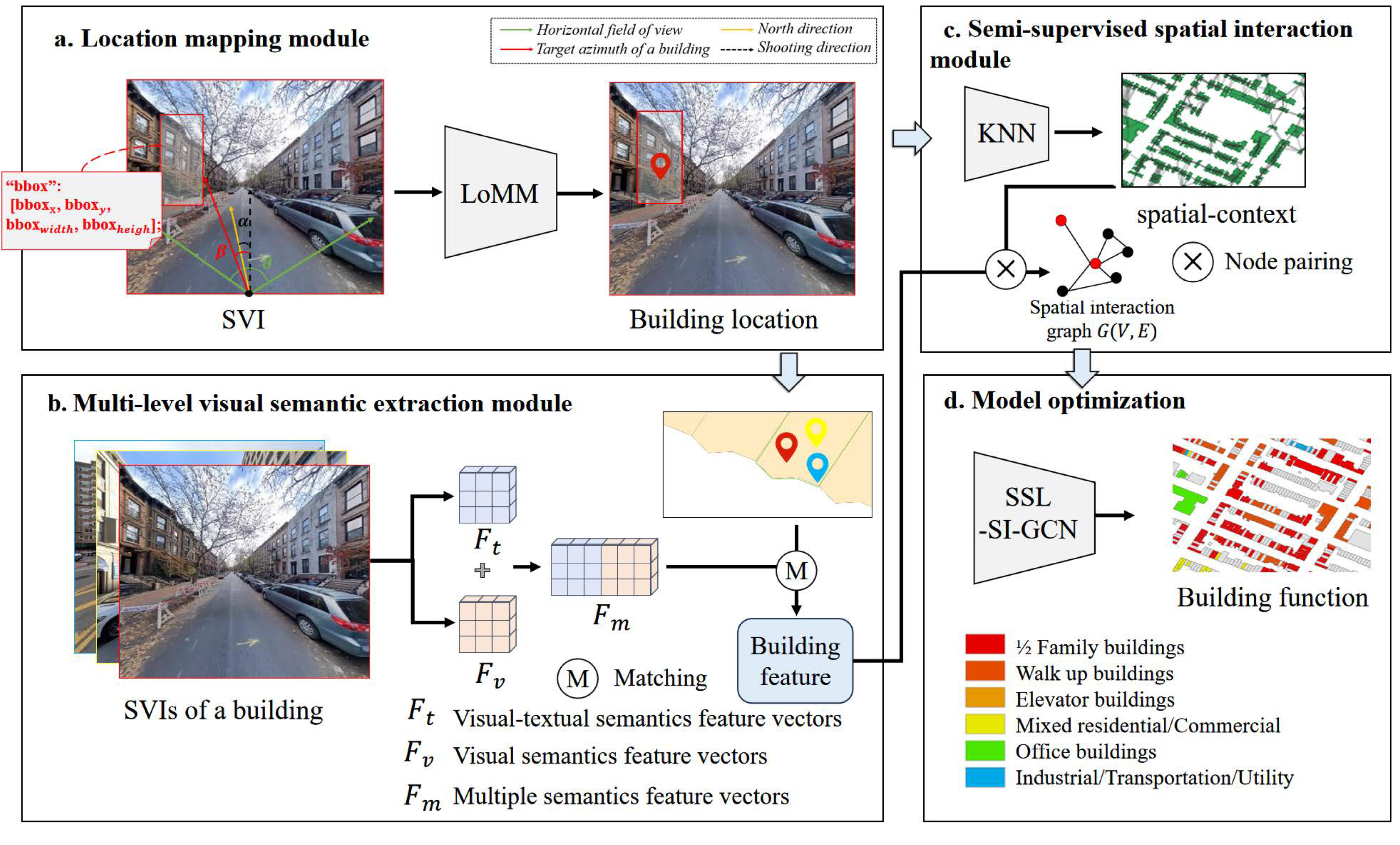
This study aims to improve building function identification by integrating multiple semantics of SVIs with the spatial context of buildings, and it proposes the multi-semantic semi-supervised building function identification (MS-SS-BFI) method. As depicted in Figure 1, the proposed method comprises four key modules: a location mapping module (LoMM) that is designed to align SVIs with buildings, a multi-level visual semantic extraction module (ML-VSEM) that extracts visual semantics and visual-textual semantics from SVIs, a semi-supervised spatial interaction module (S³IM) that integrates multi-semantics and spatial context between buildings via graph-based aggregation, and a model optimization module that trains the model and predicts the function category of each building.

3.1. Location Mapping Module

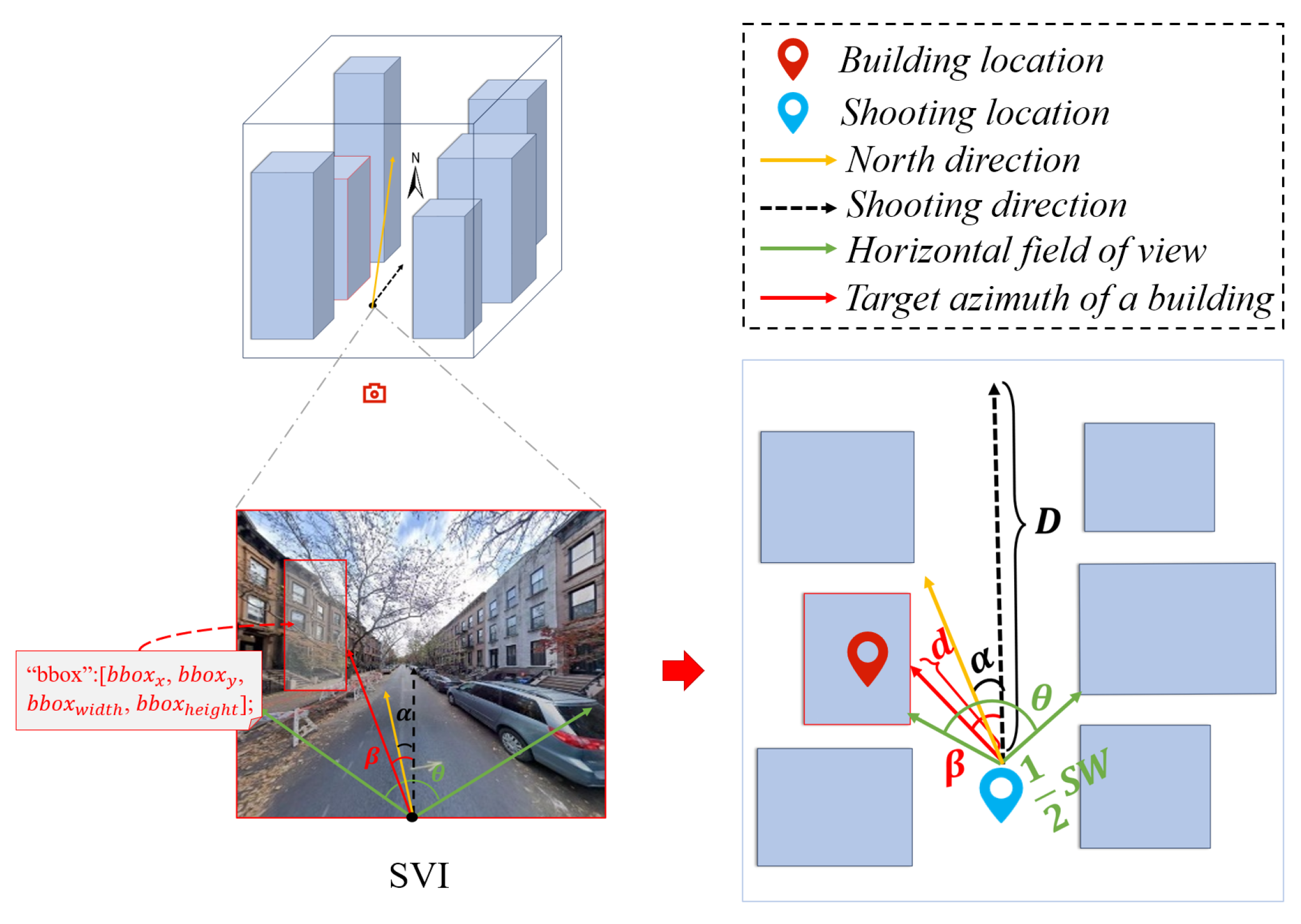
The recorded geographic coordinates of SVIs refer to the location of the camera, since SVIs are typically captured by vehicles traveling along roadways [24]. That is, the image coordinates reflect the shooting locations (i.e., where the SVI was taken), not the building locations (i.e., the true locations of the buildings). To align the image objects with building objects, the proposed method develops a location mapping algorithm. As illustrated in Figure 2, the algorithm is a three-step process.

Step 1. Calculating building azimuth $\gamma$.

The building azimuth $\gamma$ represents the angle between the shooting direction of the SVI and true north, describing the orientation of the building facade in the image. The values of $\gamma$ typically range from 0° to 360°, where 0° corresponds to true north, 90° to east, 180° to south, and 270° to west. $\gamma$ can be inferred from the SVI’s shooting direction $\alpha$ and the building’s position within the image.

The pixel position $(po{s}_x,po{s}_y)$ of the building in an SVI can be calculated using the bounding box annotations of the SVI, as shown in Equation (1):

$$\left\{\begin{array}{c}{pos}_x={bbox}_x+{\displaystyle \frac{1}{2}}{bbox}_{width},\hfill \\ {pos}_y={bbox}_y-{\displaystyle \frac{1}{2}}{bbox}_{height},\hfill \end{array}\right.$$

(1)

where $bbo{x}_x$ and $bbo{x}_y$ denote the x- and y-coordinates of the bounding box’s top-left corner, respectively; and $bbo{x}_{width}$ and $bbo{x}_{heigth}$ represent the width and height of the bounding box, respectively.

The angular deviation $\beta$ between the building and the SVI’s shooting direction can be computed using Equation (2):

$$\beta ={pos}_x\times {\displaystyle \frac{\theta }{H_{pixels}}}-{\displaystyle \frac{1}{2}}\theta ,$$

(2)

where $\theta$, estimated through multi-angle observations, denotes the horizontal field of view (HFOV) of the image; and $H_{pixels}$ is the total number of horizontal pixels in the image. $\theta$ is computed as the ratio of the difference of building azimuths ($\gamma$) to the difference in the x-coordinates of the bounding boxes’ top-left corners.

The building azimuth $\gamma$ is derived as follows:

$$\gamma =\alpha +\beta ,$$

(3)

where $\alpha$ represents the azimuth angle of the SVI’s shooting direction.

Step 2. Estimating the distance between shooting and building location.

The distance between the shooting and building location, d, is closely related to the absolute value of the horizontal offset angle. When the absolute offset angle approaches 0°, i.e., the SVI shooting direction aligns with the street’s longitudinal axis, the buildings appearing near the center of the image tend to be farther away, as they lie along the depth of the street. Conversely, when the offset angle approaches 90°, indicating a side-view perspective perpendicular to the street’s longitudinal direction, the buildings are located on both sides of the street and much closer to the camera, with the distance approaching approximately half the street width ($sw$).

To account for the fact that buildings captured at the far end of a street are not infinitely distant, this study introduces a hyperparameter, D, to denote the maximum distance from the SVI to the building. A nonlinear quadratic function is employed to represent distance variation as the building’s position shifts from the image edges toward the center. The distance d is computed as follows:

$$d={\displaystyle \frac{1}{2}}sw+{\left[{\displaystyle \frac{\theta +2fabs\left(\beta \right)}{\theta }}\right]}^2\times \left(D-{\displaystyle \frac{1}{2}}sw\right),$$

(4)

where $sw$ is a hyperparameter representing the street width, and $\beta$ is the azimuthal deviation of the building relative to the shooting direction.

Step 3. Mapping shooting location to building location.

Given the geographic coordinates of the SVI shooting location, the building azimuth $\gamma$, and the estimated distance d, the actual geographic location of the building can be inferred by solving the forward geodesic problem. The central angle $\Delta$ and deviation angle $\delta$ (in radians) are calculated by Equations (5) and (6):

$$\Delta ={\displaystyle \frac{d}{R}},$$

(5)

$$\delta ={\displaystyle \frac{360-\gamma }{360}}\times 2\pi ,$$

(6)

where R is the radius of the Earth, d is the distance between shooting and building location, and $\gamma$ is the building azimuth.

The building’s latitude ${\hat{G}}_x$ and longitude ${\hat{G}}_y$ are then derived using the Haversine formula:

$${\hat{G}}_x=\arcsin \left(\sin \left({lat}_{sl}\right)\right)\times cos\Delta +\cos \left({lat}_{sl}\right)\times sin\Delta \times \cos \left(\delta \right),$$

(7)

$$\begin{array}{cc}\hfill {\hat{G}}_y& ={lon}_{sl}+atan2\left(\sin \left(\delta \right)\times \sin (\Delta )\times \cos \left({lat}_{sl}\right),\right.\hfill \\ \hfill & \left.\cos (\Delta )-\sin \left({lat}_{sl}\right)\times \sin \left({\widehat{G}}_x\right)\right),\hfill \end{array}$$

(8)

where $la{t}_{sl}$ and $lo{n}_{sl}$ denote the latitude and longitude of the shooting location where the SVI was taken, respectively.

The complete location mapping algorithm is presented in Algorithm 1.

Algorithm 1 Location Mapping Algorithm

Input:  SVI tuple svi, Building annotations $b_{anns}$ Output:  BUILDING set buildings   1: buildings ← empty set(∅)   2: $D\leftarrow$ maximum distance   3: $\theta \leftarrow$ HOFV of svi   4: $H_{pixels}\leftarrow$ horizontal resolution of svi   5: $R\leftarrow$ radius of the Earth   6: for m ∈ SVI do   7:     BUILDING b   8:     for n ∈ $b_{anns}$ and n corresponds to of m do   9:           ${lat}_{ol}$, ${lon}_{ol}$← the latitude and longitude of m 10:           b.svfid ← the id of m 11:           ${\mathrm{pos}}_x\leftarrow$ ${bbox}_x$ + n. ${\displaystyle \frac{1}{2}}$ ${bbox}_{width}$ 12:           $\beta \leftarrow$ ${\mathrm{pos}}_x$ × ${\displaystyle \frac{\theta }{H_{pixels}}}-{\displaystyle \frac{1}{2}}\theta$ 13:           $\alpha \leftarrow$$n.heading$ 14:           b. $\gamma$←$\alpha$ 15:           b.d ←${\displaystyle \frac{1}{2}}sw$ + ${\left[{\displaystyle \frac{\theta +2·abs\left(\beta \right)}{\theta }}\right]}^2\times (D-{\displaystyle \frac{1}{2}}·SW)$ 16:           $\Delta \leftarrow {\displaystyle \frac{d}{R}}$ 17:           $\delta \leftarrow {\displaystyle \frac{360-\gamma }{\pi }}\times 2\pi$ 18:           b.Gx ←$\arcsin \left(\sin \left(la{t}_{sl}\right)\right)\times cos\Delta +\cos \left(la{t}_{sl}\right)\times sin\Delta \times \cos \left(\delta \right)$ 19:           b.Gy ←${lon}_{sl}+atan2(\sin \left(\delta \right)\times \sin (\Delta )\times \cos \left({lat}_{sl}\right),\cos (\Delta )-\sin \left({lat}_{sl}\right)\times \sin \left({\widehat{G}}_x\right))$ 20:     end for 21:     append buildings with b 22: end for 23: return buildings

3.2. Multi-Level Visual Semantic Extraction Module

Visual semantics from SVIs effectively characterize building functional features, while visual-textual semantics, derived from image captions [25], provide the scene knowledge of the SVI from pre-trained large models. These two kinds of visual semantics jointly provide complementary semantics for building function identification. As shown in Figure 3, visual semantics are first extracted using the Vision Transformer (ViT) model [26]. Subsequently, a pre-trained image captioning model generates descriptive text captions for each SVI to embed latent semantic information. Finally, the generated captions are processed by BERT [27] to extract contextualized visual-textual semantics.

Specifically, the input SVI is denoted as $X\in {\mathbb{R}}^{H\times W\times C}$, where H, W, and C represent the image height, width, and number of channels, respectively. The image is first divided into N non-overlapping patches, each of size $P\times P$. Each patch is flattened into a 1-D vector and mapped to a high-dimensional embedding space, represented as follows:

$$X_p=\left\{\begin{array}{c}{x}_p^1,x_p^2,\dots ,x_p^n\end{array}\right\},x_p^i\in {\mathbb{R}}^{(P^2·C)\times D}.$$

(9)

The embedding layer transforms these image patches into D-dimensional vectors:

$$z_0=\left\{\begin{array}{c}{x}_p^{1}E,x_p^{2}E,\dots ,x_p^{n}E\end{array}\right\}+E_{pos},E\in {\mathbb{R}}^{(P^2·C)\times D},$$

(10)

where $E_{pos}$ is positional encoding.

The embedding vectors are processed through the Transformer encoder consisting of identical L layers. Each layer employs a residual connection and layer normalization (LN) around a multi-head self-attention (MSA) mechanism, followed by a position-wise feed-forward network (MLP):

$$z_l^{\prime }=MSA\left(LN\left(z_{l-1}\right)\right)+z_{l-1},l=1,\dots ,L,$$

(11)

$$z_l=MLP\left(LN\left(z_l^{\prime }\right)\right)+z_l^{\prime },l=1,\dots ,L.$$

(12)

The visual semantic feature vectors $F_v$ are derived from the last Transformer layer:

$$F_v=LN\left(z_L^0\right).$$

(13)

Subsequently, an image caption model generates a textual description $T_v=\{{word}_1,{word}_2,\dots ,{word}_n\}$ for the SVI. The generation process is modeled as follows:

$$Pr(wor{d}_t\mid wor{d}_{1:t-1},SVI)=\mathit{softmax}({\mathbf{W}}_0·{\mathbf{h}}_t+{\mathbf{b}}_o),$$

(14)

where ${\mathbf{h}}_t$ denotes the hidden state of the LSTM at time step t, ${\mathbf{W}}_o$ represents the parameters of the output layer, and ${\mathbf{b}}_o$ is the bias term.

The textual description $T_v$ is fed into a pre-trained BERT model to encode into a semantic embedding. Let $B(·)$ denote the BERT encoding function; the resulting vector representation is

$$F_t=B\left(T_v\right).$$

(15)

Following Yang et al. [28], a concatenation-based fusion strategy integrates the visual and visual-textual semantic features. The experimental results in Section 5.5 suggest the strategy is effective.

$$F_m=f_c(F_v,F_t).$$

(16)

For each building b, let $I_b=m_1,m_2,\dots ,m_n$ denote its corresponding SVI set. The final building-level feature $B{F}_b$ is obtained by aggregating the features of all SVIs in $I_b$.

$$B{F}_b=averaging(F_{m_1},F_{m_2}\dots ,F_{m_n}).$$

(17)

3.3. Semi-Supervised Spatial Interaction Module

A semi-supervised spatial interaction graph convolutional network (S³I-GCN) is designed to integrate multi-semantics with spatial context between buildings. Specifically, a spatial weight matrix $M\in {\mathbb{R}}^{N\times N}$ is constructed to represent the spatial relationships among buildings, where n is the number of buildings. The matrix is defined as follows:

$$M_{i,j}=\left\{\begin{array}{cc}{w}_{ij},\hfill & if{v}_i\sim v_j,\hfill \\ 0,\hfill & otherwise,\hfill \end{array}\right.$$

(18)

where $v_i\sim v_j$ denotes that building $v_i$ is spatially related to building $v_j$, and $w_{ij}$ represents the spatial weight between them. The spatial weight is computed using a K-nearest neighbor (KNN) spatial weighting scheme [29], where $w_{ij}$ is inversely proportional to the distance between $v_i$ and $v_j$, typically defined as follows:

$$w_{ij}={\displaystyle \frac{1}{distance{(v_i,v_j)}^{\rho }}},$$

(19)

where $\rho$ is a hyperparameter controlling the weight decay with distance, proportional to the scaling exponent of the spatial interaction, and is set to 0 to 3 according to the spatial autocorrelation theory [30].

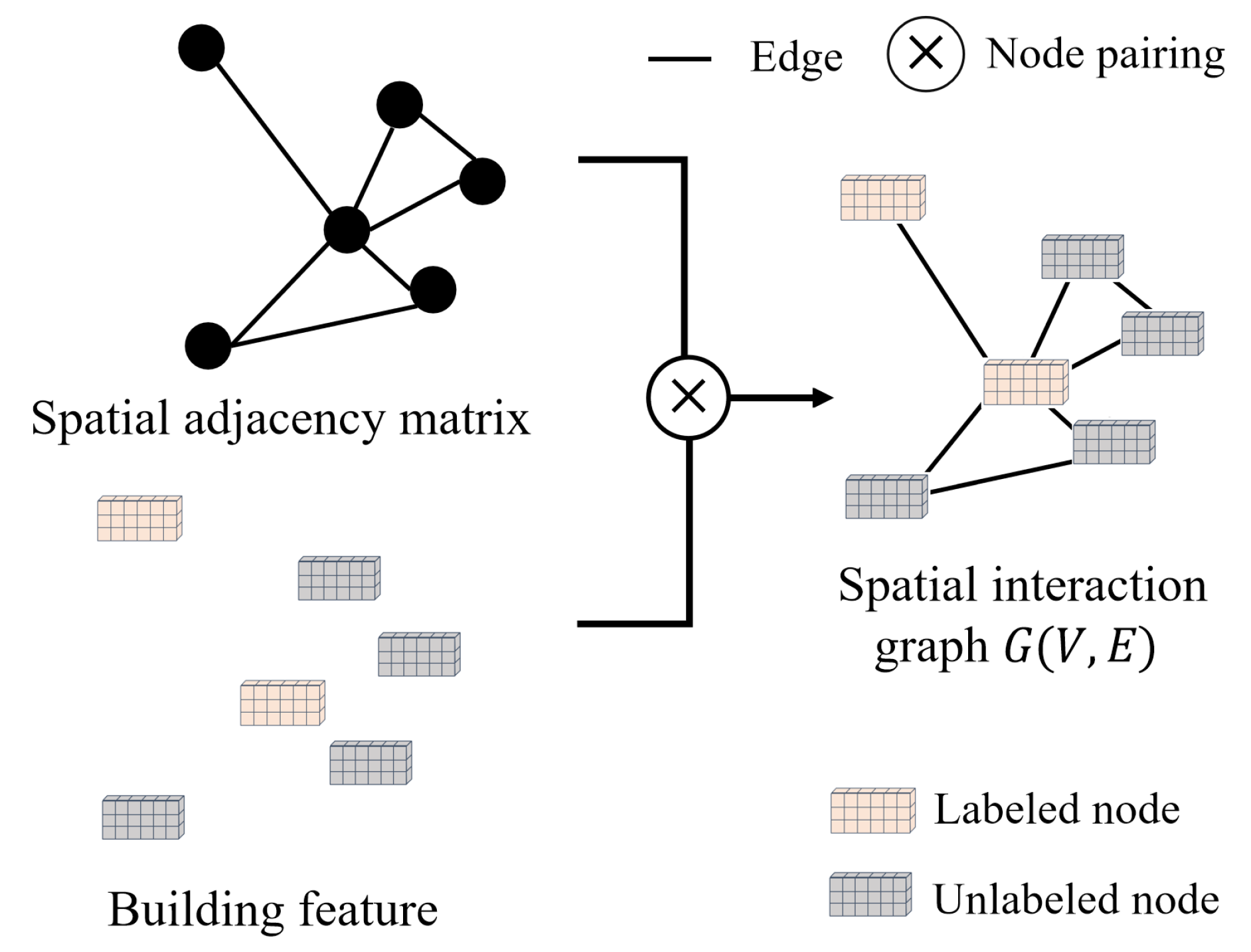
As illustrated in Figure 4, once the spatial weight matrix M is established, a spatial interaction graph $G(V,E)$ is constructed. Each node $v_i\in V$ corresponds to a building instance and is associated with a feature vector $B{F}_i$. Each edge $(v_i,v_j)\in E$ captures the spatial context between the corresponding building instances and is associated with $M_{i,j}$.

The S³I-GCN network stacks three layers of GCN to capture the relationships between nodes and their spatial interaction in graph $G(V,E)$. Each layer learns node representations by aggregating features from neighboring nodes, as formulated in Equations (20) and (21):

$$H^l=\sigma \left(\tilde{M}{H}^{(l-1)}{W}^l\right),$$

(20)

$$\tilde{M}=D^{-{\displaystyle \frac{1}{2}}}M{D}^{{\displaystyle \frac{1}{2}}},$$

(21)

where $H^l$ is the node feature matrix at the l-th layer; M is the adjacency matrix of the graph, indicating the connections between nodes. D is the degree matrix of the graph. $\tilde{M}$ is the normalized adjacency matrix, obtained by normalizing the adjacency matrix M. In semi-supervised training, the graph structure enables the propagation of label information from labeled to unlabeled nodes through feature aggregation using the matrix $\tilde{M}$.

3.4. Model Optimization

In graph $G(V,E)$, the feature matrix V, which incorporates both visual and visual-textual semantic features, is fed into the S³I-GCN. The hidden representations from the k-th layer are passed through a SoftMax classifier:

$$Z=softmax\left(h^k\right),$$

(22)

where $h^0=V$ denotes the input of the first layer.

The network is trained using a cross-entropy loss function, defined as

$$L=-\sum _{b\in y_b}\sum _{i=1}^C{Y}_{pi}ln\sigma \left(Z_{pi}\right),$$

(23)

where $y_b$ represents the set of labeled buildings in the training set, C is the number of building function categories, and $Y_{pi}$ is the ground truth label for node p and class i. Finally, the SoftMax layer outputs a probability distribution ${\left\{P_i\right\}}_{i=0}^{C-1}$ of each node over all building function categories.

4. Experimental Setting

4.1. Study Area and Datasets

This study selects Brooklyn, one of the administrative districts of New York City, as the study area. The buildings in Brooklyn are diverse in terms of type and spatial distribution. The SVIs of the study area are sourced from “Zone 2” of the OmniCity dataset [31], which provides detailed building functional categories. As shown in Figure 5, the study area covers approximately 20.09 square kilometers, and the Brooklyn dataset contains a total of 5197 SVIs. After processing by the location mapping module, 4125 unique buildings are mapped to SVIs. The SVIs and buildings are divided into a training set and a test set. The dataset is roughly divided into a training set and a test set in a 3:1 ratio. Specifically, the training set consists of 4156 images covering 3086 buildings, and the test set comprises 1041 images covering 1039 buildings. It should be noted that this paper seeks to develop a semi-supervised approach of the training model to enhance its generalization capabilities when labeled data is limited. In the experiments, the proposed method assumes that the spatial regions of training and testing data do not overlap. That is, the data used for prediction did not participate in training. Even in production scenarios where vast amounts of prediction data are available, the proposed method does not increase the training dataset size, thus alleviating computational bottlenecks of semi-supervised models.

The building functional categories in the study area include six categories: 1/2 Family Buildings, Walk-Up Buildings, Elevator Buildings, Industrial/Transportation/Utility, Mixed Residential/Commercial, and Office Buildings. A detailed description of each category is listed in

Table 1. Building function categories of Brooklyn.

Category	Abbreviation	Descriptions
1/2 Family Buildings	C1	Single or duplex family homes.
Walk-Up Buildings	C2	Low-rise, no elevator, residential.
Elevator Buildings	C3	Mid/high-rise, with elevators, residential.
Mixed Residential/Commercial	C4	Residential units above commercial spaces.
Office Buildings	C5	Business offices, multiple floors, corporate.
Industrial/Transportation/Utility	C6	Factories, warehouses, power plants, stations.

. Figure 6 illustrates each category with four samples.

4.2. Implementation Details

The pre-trained ViT model on the ImageNet dataset was employed to extract visual feature vectors from the SVIs. S³I-GCN stacks three GCN layers, connected using the ReLU non-linear activation function. The cross-entropy loss function was used to train the proposed model. The dimensions of the input layer, first hidden layer, second hidden layer, and output layer were set to 1536, 32, 16, and 8, respectively.

During training, a fixed random seed of 1,234,567 was used to ensure the reproducibility of results. The network was trained for 300 epochs using the Adam optimizer with an initial learning rate of 0.005 and a weight decay of 0.0005. In this study, K is set to 5, and $\rho$ is set to 1. The hyperparameters D and $sw$ are set to 60 and 30, respectively. Following the common setup of semi-supervised learning models, 20% of the SVIs from the training set were randomly sampled as labeled samples, and the remaining images were treated as unlabeled samples.

All the experiments were conducted using the PyTorch 2.1.1 framework and performed on a NVIDIA 3090 GPU.

4.3. Baselines

This study selected four methods as baselines to investigate the performance of the proposed method, including VGG [32], ResNet [33], StructCNN [9], and GASSL [14]. VGG and ResNet are two classical deep convolutional networks for vision tasks. VGG is known for its deep architecture that effectively captures both local and global visual features. ResNet incorporates residual learning through skip connections, allowing it to extract complex patterns of urban environments. StructCNN is a task-specific method designed for building instance classification using SVIs. GASSL is a state-of-the-art semi-supervised model of building function identification. These baselines are selected to include both classical vision models and state-of-the-art methods of building instance identification, contributing to a comprehensive evaluation of the proposed method.

4.4. Evaluation Metrics

This study adopts three widely used evaluation metrics, including Precision (Pre.), Recall (Rec.), and F1-score (F1.). For a given class, Pre. indicates the proportion of correctly predicted instances of that class among all instances predicted as that class. Rec. measures the proportion of actual instances of the class that were correctly identified by the model. F1. serves as the harmonic mean of Pre. and Rec., providing a balanced assessment of the model’s performance on that specific class.

For each class c, the evaluation metrics are defined as follows:

$$Pr{e}_c={\displaystyle \frac{T{P}_c}{T{P}_c+F{P}_c}},$$

(24)

$${Rec}_c={\displaystyle \frac{T{P}_c}{T{P}_c+F{N}_c}},$$

(25)

$$F{1}_c=2\times {\displaystyle \frac{Pr{e}_c\times Re{c}_c}{Pr{e}_c+Re{c}_c}},$$

(26)

where for each class c, $T{P}_c$, $F{P}_c$, and $F{N}_c$ represent the number of true positives, false positives, and false negatives, respectively.

The overall macro-averaged metrics are then computed as follows:

$$Pre.={\displaystyle \frac{1}{n}}\sum _{c=1}^{n}Pr{e}_c,$$

(27)

$$Rec.={\displaystyle \frac{1}{n}}\sum _{c=1}^n{Rec}_c,$$

(28)

$$F1.={\displaystyle \frac{1}{n}}\sum _{c=1}^{n}F{1}_c.$$

(29)

where n denotes the total number of classes.

5. Results and Discussion

5.1. Overall Results

As shown in

Table 2. Comparison results in the Brooklyn dataset.

Method	Brooklyn			Pre. (%) of Each Category
	Pre. (%)	Rec. (%)	F1. (%)	C1	C2	C3	C4	C5	C6
ResNet	15.64	17.35	13.43	16.67	43.06	0.00	16.92	0.00	0.61
VGG	19.30	20.42	18.53	25.69	44.28	0.00	20.33	3.57	0.00
StructCNN	20.38	19.96	19.44	20.53	49.21	2.44	22.71	4.35	1.79
GASSL	20.02	20.57	19.76	23.12	47.51	2.04	24.61	0.00	0.00
Ours	30.45	27.32	27.74	30.20	53.49	40.00	45.05	8.57	5.41

, the proposed method outperforms all the baseline models in all the evaluation metrics. Specifically, the method achieves an average Pre. of 30.45%, an average Rec. of 27.32%, and an average F1. of 27.74%, surpassing the second-best model (GASSL) by margins of 10.43%, 6.75%, and 7.98%, respectively. Additionally, the weighted F1. of the proposed method stands at 37.8%, indicating that class imbalance has affected the overall average scores. The results demonstrate the superior capability of the proposed method in accurately identifying building functions. Furthermore, the proposed method outperforms the baselines across all six building function categories in terms of Pre.; specifically, it achieves 40.00% in category C3 and 53.49% in category C2, outperforming the second-best methods by substantial margins. The improvements observed in some categories, such as C3 (i.e., Elevator Buildings), which is very challenging due to its high visual ambiguity, further highlight the effectiveness of the multiple semantics.

To further observe the performance of the proposed method, the identification results of various methods on the Brooklyn dataset are visualized, as shown in Figure 7. As illustrated in the figure, the proposed method achieves better performance compared to the baseline methods. Specifically, the baseline methods shown in columns (a) to (d) made some misidentifications. In contrast, as shown in row (e), the proposed method produces more accurate building category predictions, highlighting its superior ability when integrating multiple semantics and spatial contextual information.

5.2. Ablation Study

To further investigate the effect of each component within the proposed method, ablation experiments were conducted by systematically removing the following key components: (1) the location mapping module (w/o LoMM); (2) visual semantic features (w/o $F_{\nu }$); (3) visual-textual semantic features (w/o$F_t$); and (4) the semi-supervised spatial interaction GCN (w/o S³I-GCN). Here, “w/o” indicates that the component is removed from the proposed method. The results are reported in Figure 8.

As shown in Figure 8, when the LoMM is removed, F1. drops from 27.74% to 21.72%, indicating the importance of spatial alignment between SVIs and buildings. Removing $F_v$ slightly decreases but retains a relatively high Rec. of 26.17%, suggesting that textual semantics alone offer some resilience in classification. In contrast, removing the $F_t$ causes a pronounced decline in F1. of 19.55%, highlighting the critical role of textual descriptions in enhancing semantic discrimination. Notably, removing the S³I-GCN module leads to the most substantial performance decline, with the F1. dropping sharply to 9.26%, thereby confirming its vital role in the proposed framework. This demonstrates the critical importance of modeling spatial relationships among buildings to support robust function identification. Overall, the full model achieves the best performance, confirming that each component makes a meaningful contribution and that their integration substantially boosts the effectiveness of the proposed method.

5.3. Effect of the Training Sample Size

Given that the number of labeled training samples may affect model performance, we conducted experiments using five different numbers of labeled training samples: 10%, 20%, 30%, 40%, and full supervision (i.e., all training samples are labeled). The detailed results are presented in

Table 3. Experimental results for different proportions of the labeled sample.

Labeling Ratios	Pre. (%)	Rec. (%)	F1. (%)
10%	22.34	22.85	20.35
20%	30.45	27.32	27.74
30%	28.03	28.98	23.21
40%	25.20	23.46	23.11
Fully supervised	26.08	25.70	25.50

.

As shown in Table 3, the experimental results demonstrate that the proposed method achieved its highest F1. of 27.74% when the training sample size was 20%. Remarkably, even with only 10% of the training data, it reached 80% of the fully supervised performance, highlighting its strong applicability in low-resource scenarios. However, when the annotation ratio increased to 40%, all the evaluation metrics declined, with the F1. dropping to 23.11%. We argue this may be due to the model being trained on a large proportion of samples from the training region, which leads to overfitting and consequently lower accuracy in the test region. The results validate the effectiveness of the proposed method under limited annotated-data conditions.

5.4. Effect of GNN Models

In this study, GNNs are employed to capture and model the spatial interactions of buildings within a graph network. To evaluate the effect of different GNN models, we conduct experiments using four widely used models: Graph Convolutional Network (GCN) [34], GraphSAGE [35], Graph Attention Network (GAT) [36], and TransGNN [37].

As shown in Figure 9, GraphSAGE achieves a slightly lower Rec. of 23.22% and Pre. of 20.77%, resulting in an F1. of 18.96%. TransGNN obtains a Rec. of 24.40% and Pre. of 22.48%, resulting in an F1. of 21.06%. Overall, these results demonstrate that GCN substantially improves the model performance across multiple metrics, including Pre., Rec., and F1., by effectively capturing spatial dependencies among buildings.

5.5. Effect of Semantic Fusion Strategy

To evaluate the influence of semantic fusion strategies, we experiment with three widely used fusion methods: feature splicing, adaptive weighted average, and feature aggregation. Their results are presented in

Table 4. Experimental results for different semantic fusion strategies.

Feature Fusion Strategy	Pre. (%)	Rec. (%)	F1. (%)
Feature splicing	30.45	27.32	27.74
Adaptive weighted average	24.80	26.14	23.66
Feature aggregation	22.24	24.60	18.40

.

Among the three strategies, feature splicing achieves the best overall performance, having a Pre. of 30.45%, a Rec. of 27.32%, and the highest F1. of 30.45%. This indicates that directly concatenating visual and textual semantic features helps retain the complementary information of the two semantics, thus enhancing their discriminative capacity. In contrast, the adaptive weighted average strategy yields a slightly lower performance, having an F1. of 23.66%. The feature aggregation strategy performs the worst, having an F1. of only 18.40%. The results show that the feature splicing strategy effectively preserves the multiple semantic features, making it more suitable for building function identification tasks.

5.6. Effect of Spatial Weight

As discussed in Section 3.3, the S³I-GCN captures the influence of surrounding geographic areas on building functions by assigning weights to the edges between nodes. To investigate the effect of calculating spatial weights, we compare two commonly used methods: KNN [29] and Queen Contiguity [38]. The results are summarized in

Table 5. Experimental results for different spatial weight calculation algorithms.

Algorithm	Pre. (%)	Rec. (%)	F1. (%)
KNN	30.45	27.32	27.74
Queen Contiguity	22.99	25.06	22.96

.

Table 5 shows that KNN achieves a significantly higher F1. of 27.74%, with a Pre. of 30.45% and a Rec. of 27.32%. The improvement can be attributed to the flexibility of KNN in modeling irregular spatial structures by dynamically selecting the most relevant neighbors based on distance, thereby preserving local spatial context more effectively. In contrast, the Queen Contiguity method yields an F1. of only 22.96%, with a lower Pre. of 22.99% and Rec. of 25.06%. This suggests that relying solely on topological adjacency may overlook subtle yet relevant spatial interactions, particularly in urban environments under complex spatial distributions.

5.7. Effect of Parameter D

To evaluate the influence of parameter D on the proposed method, experiments were conducted by setting D from 40 m to 80 m in 10 m increments. The detailed results are presented in

Table 6. Experimental results for different values of parameter D.

Parameter D	Pre. (%)	Rec. (%)	F1. (%)
40 m	27.02	24.73	25.26
50 m	28.62	25.97	26.51
60 m	30.45	27.32	27.74
70 m	29.21	26.45	26.98
80 m	26.89	24.15	25.02

. As shown in this table, the highest F1. of 17.74% is obtained when D is set to 60 m. Performance declines slightly when D takes smaller or larger values, indicating that distances are either too large or too small, increasing mapping noise.

5.8. Experiments in Different Areas

To evaluate the robustness of the proposed method, an additional experiment in a different area, Wuhan city, is conducted. The Wuhan dataset covers an area ranging approximately from ${113}^{\circ }{12}^{\prime }\mathrm{E}$ to ${113}^{\circ }{41}^{\prime }\mathrm{E}$ and ${30}^{\circ }{30}^{\prime }\mathrm{N}$ to ${30}^{\circ }{39}^{\prime }\mathrm{N}$, comprising a total of 537 buildings. Each building is manually classified into one of four functional categories: Retail (C1), Apartment (C2), Office Building (C3), and Others (C4). In this experiment, the model was trained directly on samples having four-category labels.

The experiments are conducted using the same settings as those in the New York dataset. As shown in

Table 7. Comparison results in the Wuhan dataset.

Method	Wuhan			Pre. (%) of Each Category
	Pre. (%)	Rec. (%)	F1. (%)	C1	C2	C3	C4
ResNet	31.99	27.07	22.94	0.00	72.63	66.67	0.00
VGG	28.06	22.59	19.19	50.00	55.16	5.00	0.00
StructCNN	27.55	28.81	24.12	20.00	56.40	17.65	9.52
GASSL	30.59	30.78	30.25	37.04	62.41	13.33	0.00
Ours	32.21	32.56	31.27	26.67	59.46	20.00	9.52

, the proposed method outperforms the baselines, achieving overall Pre., Rec., and F1. values of 32.21%, 32.56% and 31.27%, respectively. The experimental results suggest that the proposed approach is robust.

6. Conclusions

This study highlights the importance of multiple semantics derived from SVIs for identifying building functions, and it proposes integrating multiple semantics of SVIs and the semi-supervised model to enhance identification accuracy. Specifically, a location mapping module was designed to align SVIs with buildings. Additionally, a multi-level visual semantic extraction module was developed to integrate the visual semantics and visual-textual semantics of SVIs. A semi-supervised spatial interaction module was also designed to characterize the spatial context of buildings. Extensive experiments demonstrate that MS-SS-BFI not only achieves superior prediction accuracy but also exhibits strong robustness across various scenarios. The proposed method contributes a methodological reference for SVI-based practical applications in urban analytics, especially in situations where only a small number of labeled samples are available.

Future work will focus on developing improved fusion strategies to integrate multimodal data with SVIs, thereby further enhancing the model’s identification accuracy. Additionally, it is well worth exploring the possibility of extending the proposed model by more deeply incorporating large pre-trained models that have shown strong capabilities in various visual tasks.