Article

Built-Up Surface Ensemble Model for Romania Based on OpenStreetMap, Microsoft Building Footprints, and Global Human Settlement Layer Data Sources Using Triple Collocation Analysis

by
Zsolt Magyari-Sáska
1,* and
Ionel Haidu
2,3
1
Faculty of Geography, Babeș-Bolyai University, RO-400006 Cluj-Napoca, Romania
2
LOTERR, Université de Lorraine, F-57000 Metz, France
3
STAR-UBB (Scientific and Technological Advanced Research Institute), Babeș-Bolyai University, RO-400084 Cluj-Napoca, Romania
*
Author to whom correspondence should be addressed.
ISPRS Int. J. Geo-Inf. 2025, 14(11), 420; https://doi.org/10.3390/ijgi14110420
Submission received: 6 August 2025 / Revised: 10 October 2025 / Accepted: 27 October 2025 / Published: 28 October 2025

Abstract

Accurate and up-to-date data on built-up areas are crucial for urban planning, disaster management, and sustainable development, yet Romania still lacks a unified, official database. In this study we integrated the three widely used global data sources—OpenStreetMap (OSM), Microsoft Building Footprints (MSBFs), and Global Human Settlement Layer Built-up surface (GHS)—onto a 10 m resolution raster grid and applied this consistently at the national scale across 3181 settlement polygons to produce a more accurate, unified ensemble model for Romania. The methodological basis was Triple Collocation Analysis (TCA), extended with ETC/CTC to estimate per-settlement scale factors, enabling the quantification and optimal weighting of the relative errors and accuracy in the absence of independent reference data. Weight patterns vary by settlement type: OSM receives relatively higher weights in smaller rural settlements with less redundant error; in municipalities the stronger OSM–MSBF correlation reduces both of their weights and increases the GHS share; cities exhibit a more balanced weighting. At cell level, the ensemble provides uncertainty quantification via confidence intervals that typically range from 2% to 14% at settlement scale. The resulting model—like any model—does not perfectly reflect reality; however, the ensemble improves the accuracy and timeliness of the available data. The resulting model is replicable and updatable with newer data, making it suitable for numerous practical applications, especially in spatial development and risk analysis.

Graphical Abstract

1. Introduction

Accurate, current building data underpin urban planning [1,2], health applications [3], SDG monitoring [4,5], high-resolution population models [6,7], global urban research that informs UN SDG metrics (city growth, floor space, housing) [8,9], disaster risk and emergency response (exposed structures/people) [10], and energy/infrastructure planning [11]. Yet global, standardized, up-to-date building information is hard to obtain from traditional sources, prompting reliance on open datasets—OpenStreetMap (OSM), Microsoft Building Footprints (MSBFs), and the Global Human Settlement Layer Built-up surface (GHS)—which differ in origin, methods, and characteristics; their variable quality and completeness mean that no single dataset is sufficient worldwide, motivating multi-source combination and comparison [6].
One of the recent building-related data fusion initiatives, Overture Maps, stands out as a particularly significant effort, as it aggregates footprints from OSM, Microsoft, Google, Esri community contributions, and governmental sources into a seamless global vector layer. Releases are published on a regular cadence under a transparent schema, and entities are assigned stable GERS (Global Entity Reference System) IDs to support cross-release matching and downstream data integration. EUBUCCO is another initiative to harmonize openly available governmental/administrative building datasets and, where these are unavailable, OSM. Romania is listed among the OSM-based countries, implying that much of the Romanian EUBUCCO content ultimately originates from OSM [12]. Consequently, using EUBUCCO, either for constructing the ensemble or for validation, would duplicate an input source and thus would not provide an independent reference at the national scale. A country-specific analysis is therefore essential. Romania currently lacks an open, unified, official building footprint or built-up coverage dataset [13,14], so planners, researchers, and humanitarian responders must rely on the aforementioned open sources or on remote-sensing change analyses [15]. This gap appears in pan-European compilations as well: while EUBUCCO v0.1 aggregates building footprints for EU-27 (including Romania), it documents heterogeneous completeness by country, reflecting the lack of a single authoritative national built-up source. Following Overture and EUBUCCO, a new initiative—GlobalBuildingAtlas—introduces a global vector dataset that fuses multiple footprint sources through quality-guided polygon fusion and adds building heights derived via ML on PlanetScope imagery. It draws on Google/Open Buildings, OSM, and MSBFs, and regional differences may arise in the final product depending on each source’s coverage and bias profile. [16].
Each open source offers a different picture of Romania’s building stock. Meanwhile, the country faces hazards (earthquakes, floods) and planning needs (infrastructure expansion, heritage conservation) that require reliable building data [17,18,19,20]. Understanding the coverage and accuracy trade-offs among OSM, MSBFs, and GHS will allow for improved risk modeling—for instance, estimating earthquake exposure requires reliable information on the proportion and spatial distribution of built-up area within hazard zones. A focused study in Romania can therefore assess these datasets under local conditions and guide Romanian GIS users and policymakers on when to rely on each source.
The aim of this study is to present a data fusion of the three sources for Romania, producing a 10 m resolution raster product in which each grid cell estimates the proportion of built-up area which is appropriate given the mixed vector/raster inputs and the national scale of the analysis. The main challenges are uneven completeness, source-specific biases and correlated errors between input datasets. We address these by using a settlement-aware Extended/Correlated Triple Collocation (ETC/CTC) approach that rescales inputs per settlement, models cross-covariances, and yields best linear unbiased weights with quantified uncertainty. Our contribution is twofold: the first country-wide, settlement-level ensemble for Romania; and the application of Triple Collocation Analysis (TCA) to combine these specific sources in this context, providing weights and uncertainty layers that support risk and planning use-cases.

2. Materials and Methods

2.1. Data

Three data sources on urban built-up areas were used for the analysis: the OSM community-developed vector dataset, the MSBF vector dataset derived from satellite remote-sensing, and the GHS raster dataset, also generated from remotely sensed data.
As OSM is a community-developed crowdsourced database, its open-data policy makes detailed building data with location information available in many places. However, coverage is highly uneven: a global study found that in nearly half of city centers less than 20% of buildings are included in OSM, while in some cities in wealthier countries, more than 80% are included [8,21]. OSM completeness was measured using MapSwipe [22] and by comparison with GHS. These studies suggest that in many countries in Africa, Asia, and South America, only a small percentage of buildings are included [23]. In Romania, for example, the approximately 2.1 million OSM buildings cover only 15–20% of the actual stock [24]. We used the Geofabrik Romania OSM extract, which supplies a country-bounded, regularly updated dataset with complete building geometries (including polygons with holes), enabling a transparent, reproducible pipeline. The “buildings” layer prepared by Geofabrik consists of all objects tagged building or building part, represented as polygons or multipolygons.
MSBF is a machine-learning-derived database of automated building footprints from high-resolution aerial and satellite imagery, launched in the US in 2018 and made available globally. The 2022 release contains around 856 million building contours worldwide, rising to roughly 1.4 billion by 2024 [25]. The dataset also covers Romania, with approximately 13–14 million buildings, compared to a much smaller OSM dataset of a few million [26]. MSBF can substantially increase completeness, especially in countries where OSM is under-mapped (e.g., Romania) [24]. The automated method provides large and relatively uniform coverage, but it has limitations: geometric errors due to machine vectorization, positional inaccuracies, and misidentifications may occur. Comparative studies show that building counts are mostly consistent, but differences in the polygonization of complex shapes occur [25]. In the MSBF dataset, polygons, which would conventionally be modeled as ringed geometries (i.e., with interior holes) are not encoded as topological shells with inner rings. Instead, MSBF represents such features as single-shell polygons that enclose interior voids (e.g., courtyards), thereby subsuming spaces surrounded by buildings within the outer footprint boundary.
GHS is a global dataset from the European Commission’s Joint Research Centre that maps human presence (built-up area, population, etc.) in a comparable way over time. The GHS layer provides the proportion of built-up area in each cell [27]. Several time series were produced by machine-learning processing from Landsat, Sentinel-2, and other satellite imagery, covering 1975–2030. As an open, standardized, and globally consistent dataset, GHS often serves as a base layer whose accuracy is continuously improved [28], and against which more detailed datasets (e.g., OSM, MSBF) can be compared. However, the GHS does not separate individual buildings, and its resolution can be inaccurate in rural, sparsely built-up areas. Validations show that it underestimates sparse built-up areas, while in dense urban cores it tends to overestimate built-up areas. A study in Chinese cities reported good correlations with actual built-up areas, but underestimation in scattered developments and overestimation in dense blocks [29]. For Europe, compared with an integrated building map, the GHS 10 m grid overestimated built-up area by ~47% overall; scaling to 0.68 brought it in line with the actual footprint [24].
OSM, MSBF, and GHS represent three different paradigms for mapping built-up coverage. OSM provides fine detail and local knowledge, MSBF provides broad coverage and machine consistency, while GHS provides full global coverage and time-series depth. All three have shortcomings in completeness or accuracy, so comparing them and transforming them into an ensemble model yields a more robust result than any single dataset alone. The OSM and MSBF layers, originally in vector format, were reprojected to the Mollweide projection used by GHS and rasterized to 10 m resolution, aligned to the GHS grid origin (Table 1).
For the comparison of settlement built-up area with population, we used registered population data from the Romanian National Statistical Office’s (RNSO) TEMPO database as of 1 January 2025 (POP107D section). The use of the 2018 GHS layer does not undermine the reliability of the planned analysis compared to the time-heterogeneous OSM and MSBF inputs. Independent validations reported an overall class accuracy of 91% for 44 000 points in the built/unbuilt binary test [30]. The “freshness” of the OSM and MSBF layers is only apparent, as the volunteer edits are from different years within a municipality, and MSBFs are derived from imagery with varying time stamps across countries between 2017 and 2025. In other words, these layers are multi-temporal and therefore do not serve as a real-time reference standard compared with GHS. The methodology discussed in the next subsection addresses temporal discrepancies: the TCA procedure estimates per-settlement scale and error factors for systematic differences between sources, including time drift, without reference measurement.

2.2. Methods

Merging OSM, MSBF, and GHS datasets in the absence of ground truth poses a classic data-fusion problem: how to combine multiple, partially overlapping sources of different reliability in a way that yields a consensus with quantified uncertainty. TCA is a commonly used option, but the literature also offers several alternative or complementary approaches.
Bayesian Ensemble Modeling combines sources with probabilistic weighting, but in the absence of prior reliability assumptions or calibration [31,32], weights can be subjective and shared biases can hide true errors; without reference data, modeling assumptions are sensitive and difficult to validate. The Dempster–Shafer theory can combine incomplete or contradictory signals [33,34], but the design of basic probability assignments and fine-tuning of conflict handling are often ad hoc. Correlated evidence can bias the results, and the original rule sets have well-documented weaknesses that various extensions attempt to address. A machine learning ensemble model can learn internal consistency, but without ground truth it easily amplifies common biases and overfit and produces combined results that are difficult to interpret or validate [35]. Hierarchical weighted overlay or MCDA (Multi-Criteria Decision Analysis) approaches are transparent and work with expert weighting [36], but the weights are often subjective and sensitive to definitions, and it is difficult to separate random and structural errors without a reference.
Each alternative may provide additional value, but each also relies on stronger assumptions or components that are difficult to calibrate in the absence of a reference. It is therefore useful to employ a diagnostic method with relatively few assumptions—TCA/ETC/CTC—to obtain empirical error and weight estimates and to incorporate this information into the above fusion mechanisms as needed. We chose TCA because it provides objective weighting in a reference-free situation. It is a statistical framework that can provide unbiased estimates of random-error variances and scaling factors relative to a “real” but imprecise measurement by jointly examining three statistically independent estimates of the same physical signal. The method is particularly useful when reliable reference measurements are lacking, the signal under investigation has a large spatial or temporal extent, and three instrumentally-, data source-, or data processing algorithm-independent datasets are available. TCA and its extensions have been successfully applied to determine sea wind and wave height [37], soil moisture [38,39,40,41,42], surface cover accuracy [43], sea ice thickness [44], evaporation [45], and precipitation [46,47,48].
The underestimation of OSM and the overestimation of GHS are addressed by TCA scale factors, which typical deterministic methods do not correct. The classical approach assumes a linear, additive error model (Equation (1)), whereas ETC addresses both error correlation and signal-error dependence [49]. TCA estimates scale factors and error variances for three statistically independent datasets measuring the same unknown true signal, without a reference.
x k = α k s + e k , k = 1,2 , 3
s—ground truth
xk—measured value
ek—additive random error
α k—scale factor
Since the cross-covariances in the covariance matrix of the three measurements (Equation (2)) do not contain an error component, they can be used to calculate the scale factors (α) (Equation (3)) and the error variances (σ2) (Equation (4)). Per-settlement scale factors correct source-level differences prior to weighting; this rescaling is estimated from the data and thus also mitigates discrepancies that can arise from non-contemporaneous acquisition among sources.
C O V = c 11 = α 1 2 σ s 2 + σ e 1 2 c 12 = α 1 α 2 σ s 2 c 13 = α 1 α 3 σ s 2 c 21 = α 1 α 2 σ s 2 c 22 = α 2 2 σ s 2 + σ e 2 2 c 23 = α 2 α 3 σ s 2 c 31 = α 1 α 2 σ s 2 c 32 = α 1 α 2 σ s 2 c 33 = α 3 2 σ s 2 + σ e 3 2
α 1 = c 12 c 13 c 23 ; α 2 = c 12 c 23 c 13 ; α 3 = c 13 c 23 c 12
σ e 1 2 = c 11 α 1 2 ; σ e 2 2 = c 22 α 2 2 ; σ e 3 2 = c 33 α 3 2
From these calculated values, after calibrating the scale factors, the best linear unbiased estimate (BLUE) with the smallest variance ( s ^ ) can be obtained as an error-inverse weighted average (Equation (5)).
s ^ = k = 1,3 w k y k ; w k = 1 σ e k 2 j = 1,3 1 σ e j 2 ; y k = x k α k
The uncertainty of the estimated value is given by the standard deviation of the error (SD( s ^ )) (Equation (6)), which will give the confidence interval.
S D s ^ = k = 1,3 w k 2 σ e k 2
If the three data sources are not completely independent from each other (e.g., data and/or methodological dependencies between two data sources), error variances can be derived using CTC equations of Gonzales-Gambau [50] (Equation (7)), and the weight vector values (w) are computed via Equation (8) (for the case in which sources 1 and 2 are correlated). In our settings, GHS and MSBF share remote-sensing origins and are treated as correlated.
σ e 1 2 = c 11 1 ρ 12 2 c 12 2 c 22 2 ρ 12 c 12 + c 11 ; σ e 2 2 = c 22 1 ρ 12 2 c 12 2 c 11 2 ρ 12 c 12 + c 22 ; σ e 3 2 = c 33 c 13 c 23 ρ 12 c 12 c 33 c 11 + c 22 2 ρ 12 c 12
ρ 12 —data sources’ error correlation
w = e 1 1 1 T e 1 1
1—unity vector
Σ e 1 —error covariance matrix inverse
The built-up estimate in a given cell site is given by Formula (9).
w O S M · x O S M + w M S B F · x M S B F + w G H S · x G H S
The complete workflow per settlement follows the steps below:
Preprocess: We align the data sources on the common 10 m grid and settlement mask, rasterize the OSM/MSBF sources, and center each source by removing its settlement mean. Centering isolates covariation around the local signal and prevents mean offsets from biasing scale/variance estimates.
Estimate scaling: Using ETC on the centered triplet, we estimate per-source scale factors that map each input to a common latent signal scale. These factors correct systematic amplitude differences (e.g., under/overestimation) before any weighting.
Estimate errors with correlation: We then apply CTC to the rescaled triplet to obtain error variances and the cross-covariance term that captures known dependence between the GHS and MSBF datasets. This yields a settlement-specific error covariance matrix.
Compute BLUE weights: for pixels where all three sources are non-zero, we compute BLUE weights by inverting the error covariance. This provides data-driven weights and a combined built-up estimate on the common scale.
Handle zeros and missingness: When an input is zero while peers are non-zero, we treat it as missing for weight estimation. When one of the sources does not show built-up coverage in a given cell, but the other two do, the existence of the building is still probable (e.g., an OSM absence may reflect unmapped buildings; a GHS absence may reflect acquisition timing). In such cases, the original TCA-based weights are rescaled. Because OSM generally offers high positional accuracy where present, its weight is explicitly constrained in the algorithm in two-source cases. When built-up is indicated by a single remote-sensing-based source (GHS or MSBF), considered as a more error-prone situation, we treat presence as uncertain and reduce the TCA-derived contribution by a preset division factor, remaining conservative until corroborated by additional sources. Although the used parameter values have empirical motivation, they remain partly subjective. We therefore assess their impact using a Morris sensitivity analysis.
Propagate uncertainty to confidence intervals. For each pixel, we combine the weights with the estimated error variances to compute the standard error and report confidence intervals for the ensemble estimate, enabling uncertainty-aware interpretation and downstream use.
The Morris method [51] ranks the effects of input factors using fast calculations and indicates which factors behave nonlinearly or interact. For this, it calculates elementary effects based on Equation (10).
E E i x = f x 1 , , x i + , , x k f ( x )
f(x)—model output
xi—ith factor value
Δ—step value
The characteristics of the ith factor are the mean effect μ i , the effect size μ i , and the standard deviation of the effect σ i , calculated from r different starting points [11].
μ i = j = 1 r E E i r μ i * = j = 1 r E E i r σ i = j = 1 r ( E E i μ i ) 2 r 1
The σii* ratio indicates volatility and context-dependence: low values suggest near-linear, stable behavior; high values suggest a complex or interactive effect. This ranking guides which factors merit further investigation.
The methodology was implemented in R (version 4.5.1) and is publicly available in a GitHub repository https://github.com/zsmagyari/Romania_BuildingFootprint (accessed on 8 October 2025).

3. Results

Applying TCA at the settlement level reduces spatial heterogeneity (OSM completeness varies by settlement) and strengthens the validity of the basic assumption that the three independent data sources truly refer to the same real-world entity [52,53,54,55]. We therefore applied the method at the settlement level, using Romania’s Level 3 administrative boundaries, for a total of 3181 polygons. Romanian Level 3 units are Local Administrative Units (LAUs), which encompass compact urban cores as well as surrounding agricultural or natural areas.
GHS and MSBF provide full spatial coverage, so a value of “0” always reflects an absence of buildings at the sensor’s observation time, not a lack of data. By contrast, in OSM a value of “0” may indicate either unmapped areas or a genuine absence of buildings. It is worth noting that OSM’s data gaps are not comparable—either in quantity or spatial extent—to the possible shortcomings of MSBF or GHS: for the latter, omissions arise mainly from sensor limitations or post-processing detail, and the affected area is typically orders of magnitude smaller than in OSM. Results from the initial test phase support this observation. Figure 1 shows that treating OSM zeros as true absences can locally bias the ensemble output (ENS).
To ensure that ETC estimates weights only from relevant existing data, we flagged cells as missing (NA) where OSM had a value of 0 and both GHS and MSBF reported data; these cells were excluded from the three-source analysis to minimize bias from mapping gaps. In applying ETC and computing weights, we considered only cells with positive values in all three data sources. This filtering step ensured that subsequent analyses relied on genuine, reliable settlement coverage. Using the ETC procedure implemented in R, we computed the pairwise covariances of the three data sources (Xᵢ), from which we estimated each source’s error variance and relative scale factor (αᵢ). After bias correction (Equation (12)), the bias-corrected data matrices (Xᵢ*) were obtained using Equation (13).
b i = X i α i T 0 ¯ T 0 = 1 3 i = 1 3 X i α i
X i * = X i b i α i
The bias-corrected matrices were then processed with CTC, which yields an error–covariance matrix, including estimated error correlations between sources. Source weights were derived under the BLUE criterion, minimizing the variance of the combined estimate. Where all three data sources were available, these three-source weights were used to compute the cell values. When OSM was missing, the GHS and MSBF weights obtained from CTC were renormalized to sum to one, and these normalized weights were used to estimate the ensemble value for that cell. When exactly two sources indicated built-up area and one of them was OSM, we applied a presence-privileging fallback: 0.95 for OSM and 0.05 for partner source, interpreting an explicit OSM polygon as higher-specificity evidence than a remote-sensing detection. If only OSM indicated built-up area (single-source case), we likewise assigned 0.95 to OSM. In contrast, if only GHS or only MSBF indicated built-up area, the settlement-level weights originally determined by the ETC/CTC procedure were down-weighted using source-specific correction factors with default value 3 to remain conservative until corroboration was available. A sensitivity analysis, presented in the Discussion, was performed for all three correction parameters to quantify their influence on the final results.
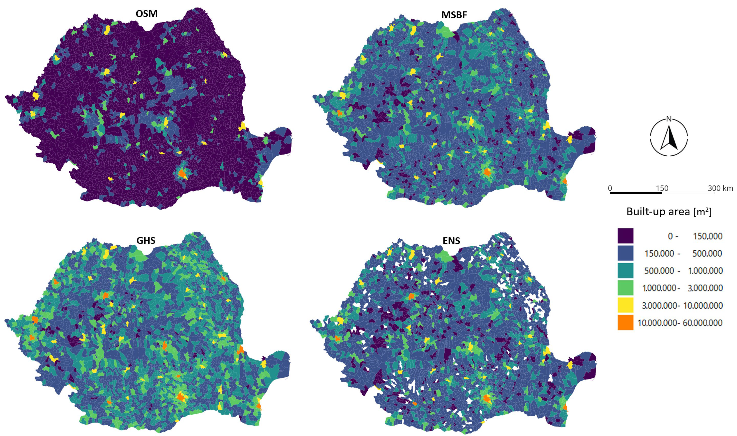
The OSM data source did not contain any buildings for 208 settlements due to incomplete coverage, so the ETC/CTC procedure could not be applied in those cases. The OSM built-up pattern is highly concentrated: medium or higher coverage appears mainly in large cities—such as the Bucharest area and several regional centers—indicating uneven national coverage (Figure 2, OSM). By contrast, MSBF generally identifies more built-up area with markedly more homogeneous spatial coverage, although prominent urban centers remain visible (Figure 2, MSBF). The GHS layer indicates higher built-up coverage in most settlements and yields a more uniform, intensive picture with much less regional variation; this pattern is consistent with a lower spatial resolution but consistently applied methodology (Figure 2, GHS). The three data sources have distinct error structures, a precondition for effective TCA weighting. The ensemble output consistently combines and harmonizes the three sources, yielding a more reliable, integrated estimate (Figure 2, ENS). White areas indicate locations where OSM data are completely missing.
At the settlement level, Figure 3 presents the small town of Gheorgheni, where the built-up values of the three data sources are balanced (OSM: 1.19 sq. km/GHS: 1.78 sq. km/MSBF: 1.32 sq. km). After the ETC/CTC analysis, the resulting weights were OSM: 13%/GHS: 77%/MSBF: 10%. The three example sites in Figure 3 highlight the effectiveness of the ETC/CTC algorithm for this town. Case A is a currently unused complex, a former industrial facility that appears in OSM and GHS, but is only partially identified by MSBF. The ensemble successfully fills its missing part in MSBF. Case B is the city’s most important high school: it is present in OSM and GHS, but absent from MSBF. The fact that it was built in 1914 illustrates that this omission is not attributable to dataset recency, but rather to coverage or extraction limits. The ensemble successfully fills this gap. Case C is the city’s central park, which is surrounded by buildings but contains no built-up are within its bounds. OSM and MSBF reflect this, whereas GHS overcompensates and marks several areas of the park as built-up. The ensemble successfully corrects this and recovers the park’s triangular shape.
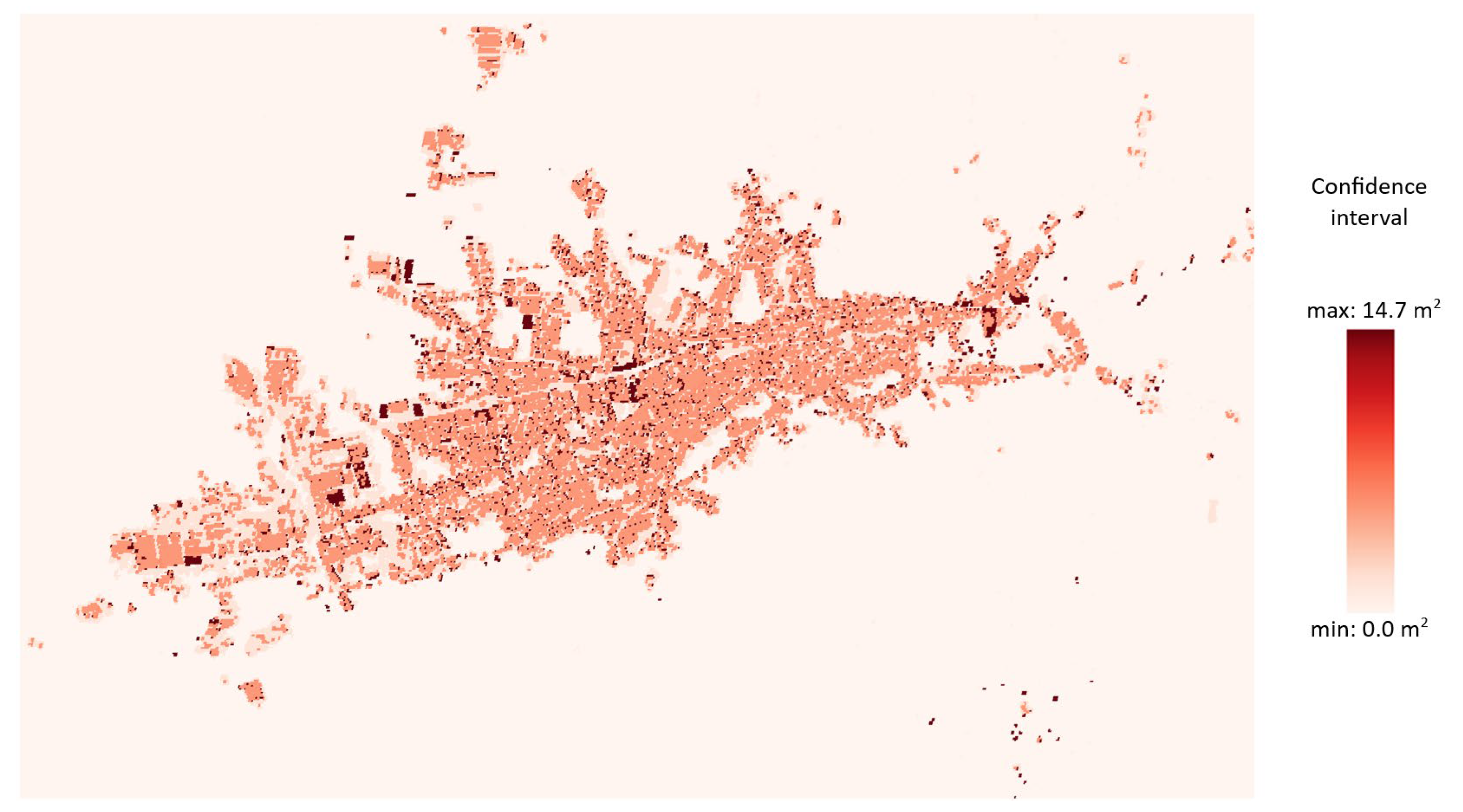
Because nationwide ground-truth data were unavailable, direct validation was not possible. Instead, we computed a confidence interval for each model output, whose width depends primarily on the number of sources contributing to a pixel. For Gheorgheni, the confidence-interval mean width is 7 m2, indicating that the ensemble estimate may deviate by up to about 7% (Figure 4). Visual checks also support the ensemble’s applicability: whereas GHSL often assigns non-zero built-up values to normal-width roads, the ensemble substantially corrects and reduces these cells’ value based on MSBF and OSM (Figure 5). The Supplementary Material also includes three visual-validation case studies from different regions of Romania.
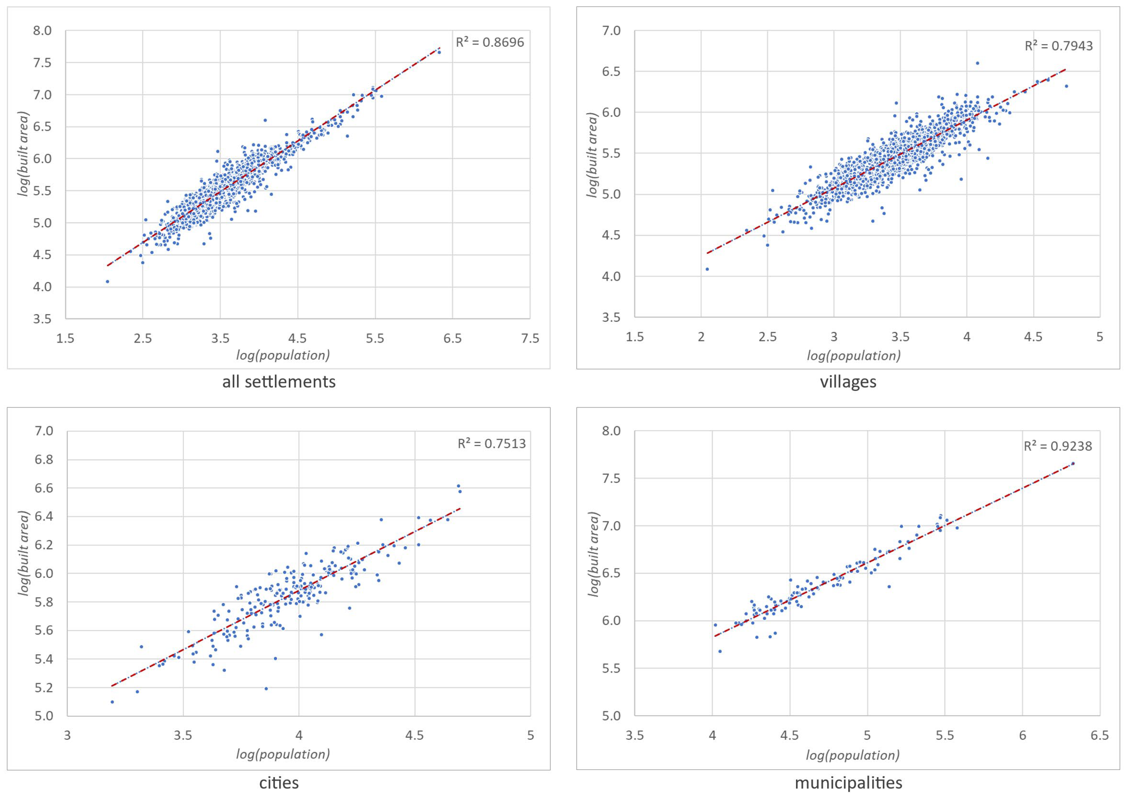
In addition to visual inspections, we applied two indirect validation approaches. The first leverages the expected close relationship between population and built-up area, illustrated in Figure 6 on a log–log scale for both variables. We conducted the correlation analysis across all settlements and separately by settlement type: 2656 rural settlements (villages), 215 cities, and 103 municipalities (high-ranked cities), including the capital. Municipalities show higher correlations than the other types with a difference of 0.13–0.18, consistent with more homogeneous built-up structure.
As a second validation element, we drew on a key literature-based value associated with GHS. Florio [24] reports that applying a 0.68 correction factor to GHS brings estimates in line with actual built-up coverage. Our comparison of the ensemble’s built-up area with GHS (Figure 7) yields very similar ratios, with slightly higher values for municipalities.
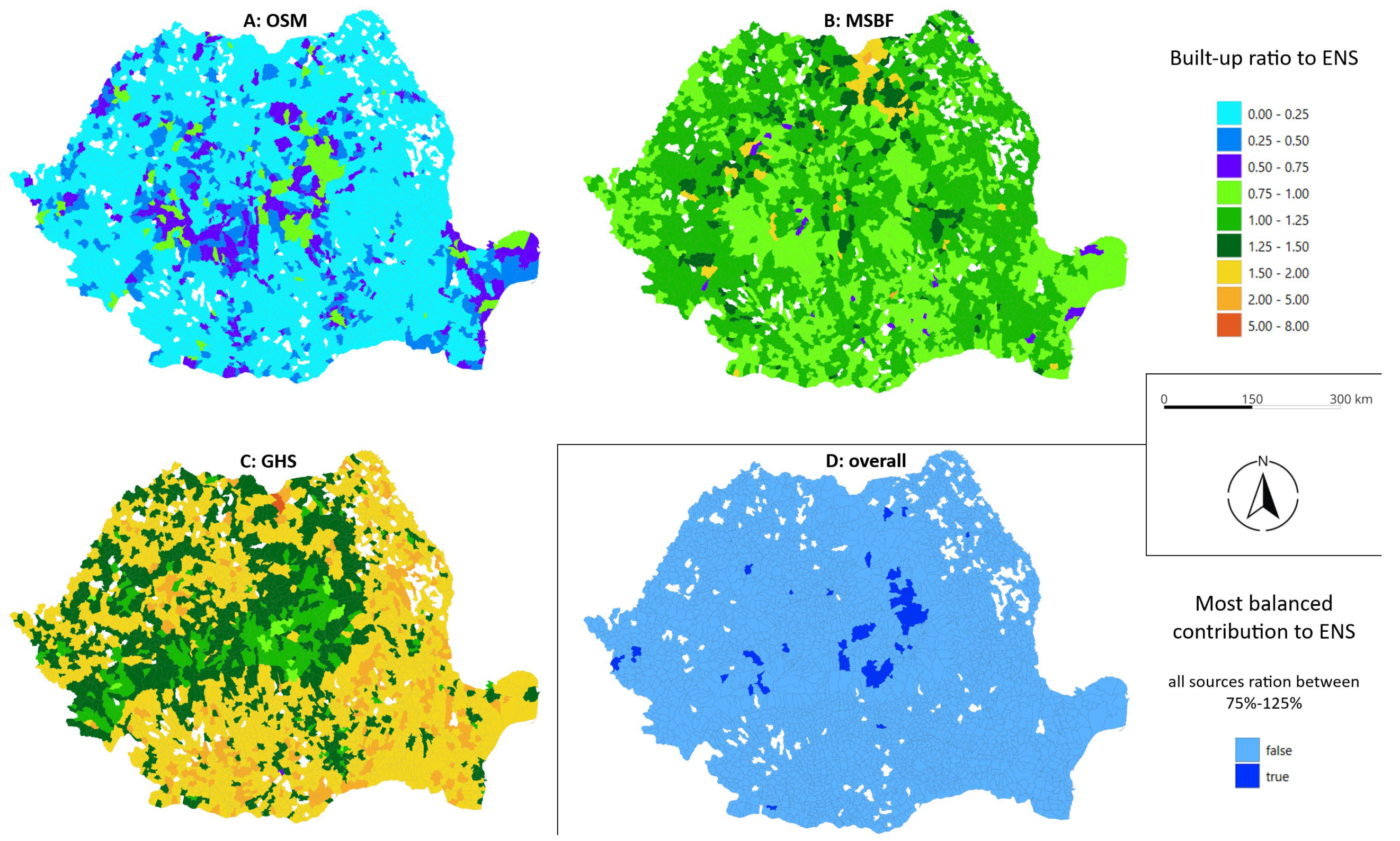
Figure 8 uses the ensemble as a reference and shows each source’s proportional contribution. OSM coverage is most significant in the country’s central regions and in large cities. MSBF falls within 75–125% of the ensemble across most of Romania, with exceptions in the north—particularly in Suceava County—and in scattered mountainous settlements of the Carpathians. GHS typically overestimates built-up area over large parts of the country, except in the central region and in some settlements of the Southern and partly Western Carpathians. Panel D highlights the settlements where all three sources fall within the 75–125% band relative to the ensemble.
The ensemble model for the entire territory of Romania is available in Zenodo, together with the R code used to generate the database and example data on GitHub https://github.com/zsmagyari/Romania_BuildingFootprint (accessed on 8 October 2025).

4. Discussion

ETC/CTC produces an ensemble model from three independent data sources. However, for the OSM layer the meaning of zero is ambiguous, so cells where OSM is zero while the other sources report data were excluded from weight estimation. This is a limitation: locations that are truly built-up but unmapped in OSM do not contribute to determining the weights. Consequently, the ensemble is expected to be most accurate in settlements where all three sources provide non-zero and comparable signals. The same logic applies within settlements: in areas where all three sources are non-zero, ensemble estimates are more reliable.
OSM occasionally ingests external datasets via documented community imports (e.g., governmental inventories, MSBF). Consequently, OSM building data are not guaranteed to be fully independent of other inputs used in this study, and pairwise error correlations may arise. In the present implementation we model the cross-covariance among the remote-sensing-derived sources (GHS–MSBF) and apply a conservative fallback weighting in two-source pixels to limit over-reliance on potentially dependent pairs. The open workflow can be extended to include additional cross-covariance terms where local evidence warrants it. The CTC/ETC framework is capable of estimating additional cross-covariances, and our open code can be extended accordingly in future releases.
The analysis shows substantial within-category variation in weights (Figure 9). Overall, OSM tends to receive a higher weight—and thus greater importance—than the other two sources. In small settlements with limited volunteer mapping, the non-zero OSM cells are often more accurate and less correlated with GHS or MSBF, which provide full coverage. Because OSM’s errors are less redundant in these places, its relative weight exceeds that of the other sources. In cities, particularly in densely built-up areas, OSM, MSBF, and GHS often produce similar estimates because all three track built-up areas detail. Their errors are therefore strongly correlated, which reduces the weight of each source—ETC/CTC avoids overvaluing redundant information by not assigning a particularly high weight to sources that resemble one another. In municipalities, the OSM–MSBF correlation is most pronounced; as a result, their weights decline, and the GHS contribution increases, reflecting its comparatively lower correlation with the other two.
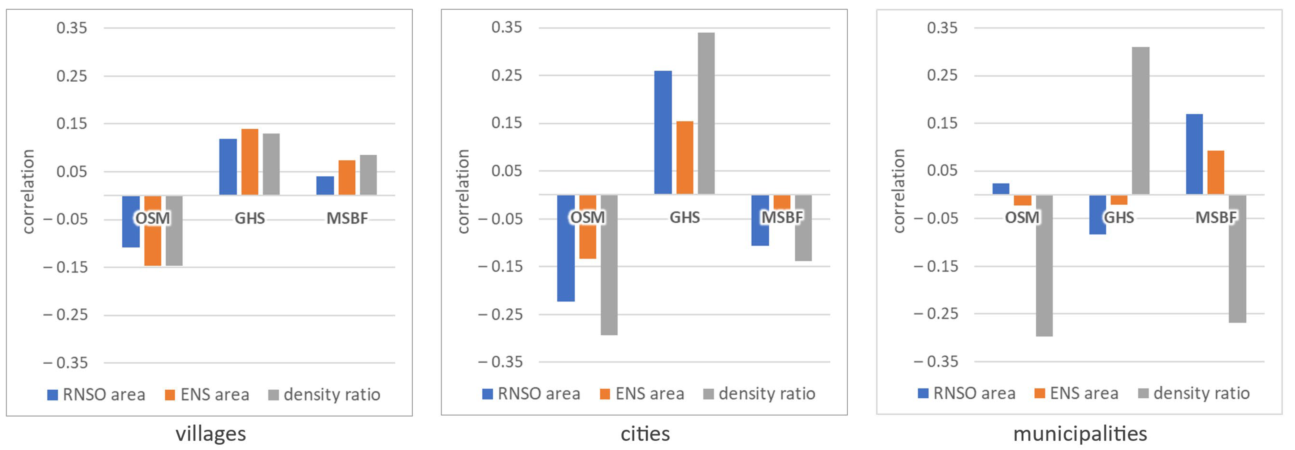
To analyze why weights differ by settlement type, we computed three settlement-level metrics: residential floor area (from RNSO), the ensemble built-up fraction (share of 10 m cells classified as built-up within each settlement), and a jurisdictional built-up ratio defined as ensemble built-up area divided by the entire administrative area. We then related the obtained weights to these metrics within each settlement type (villages, cities, municipalities) using Pearson correlations (Figure 10). Across villages, the obtained correlations are weak but directionally consistent for all three metrics: the OSM weight decreases slightly with built-up area, the GHS weight increases, and the MSBF weight is near-neutral to mildly positive. In cities, the relationships strengthen: OSM weight declines with higher built-up area, GHS weight increases, and MSBF weight modestly decreases. This aligns with our interpretation that GHS performs better in compact, high-density urban fabrics, whereas OSM/MSBF become more redundant as density rises. In municipalities, total built-up area extent is close to saturation, hence correlations with INSSE data the and ensemble fraction are near zero. By contrast, the jurisdictional built-up ratio reveals the operative mechanism: GHS weights rise in more compact jurisdictions, while OSM and MSBF weights decline, indicating that in very large cities the key determinant is structural compactness of the jurisdiction, not sheer built-up extent. The fact that both the official (RNSO) and ensemble measures reproduce the same correlation directions strengthens confidence in this interpretation.
Our city-type dependent weights mirror known data-quality patterns: global analyses show large heterogeneity in OSM building completeness—typically highest in large, high-SHDI urban centers and markedly lower elsewhere—so where OSM coverage is strong our ensemble assigns it greater influence, while down-weighting it in smaller towns [8]. In compact urban cores, we observe higher contributions from 10 m GHSL/GHS-BUILT-S2 layers, consistent with recent assessments that report strong spatial accuracy but settlement-type-dependent variation in gridded built-up products [56]. Conversely, in dispersed rural settings, vector footprints (e.g., Microsoft Building Footprints: high-precision where available) can capture small, isolated structures that coarser gridded layers may undercount, and our ensemble correspondingly shifts weight toward these sources when local validation supports their coverage [57].
The 0.95 OSM fallback is not a global preference but a guardrail used only where CTC cannot operate, privileging object-level presence over a lone remote-sensing hit (GHS or MSBF) while avoiding hard switches. Morris screening indicates that the OSM weight is not the dominant driver in most settlements. Accordingly, choosing OSM weight at 0.95 is conservative with limited impact on aggregate outcomes. As OSM building completeness is uneven across cities and regions, Romania’s LAU often mix well-mapped urban cores with sparsely mapped rural peripheries. In our ensemble, such intra-LAU heterogeneity manifests as broader confidence intervals and lower effective weights for uncertain sources, while stable, well-mapped areas exert greater influence. Within the ETC/CTC framework, constant cross-source-level differences at the LAU scale are absorbed by the scale factors, whereas spatially varying differences inflate the error variances and are therefore down-weighted in the BLUE combination.
We evaluated this fallback logic with sensitivity analysis also when only GHS or only MSBF was available; we reduced their contribution using two- to five-fold attenuation to remain conservative until corroboration was available. These bounded values were the levers explored in the analysis: smaller GHS or MSBF reductions make single-source “islands” more assertive (higher false-positive risk), while larger reductions render them more tentative (higher false-negative risk). In all cases, impacts are localized to fallback pixels, not the entire map.
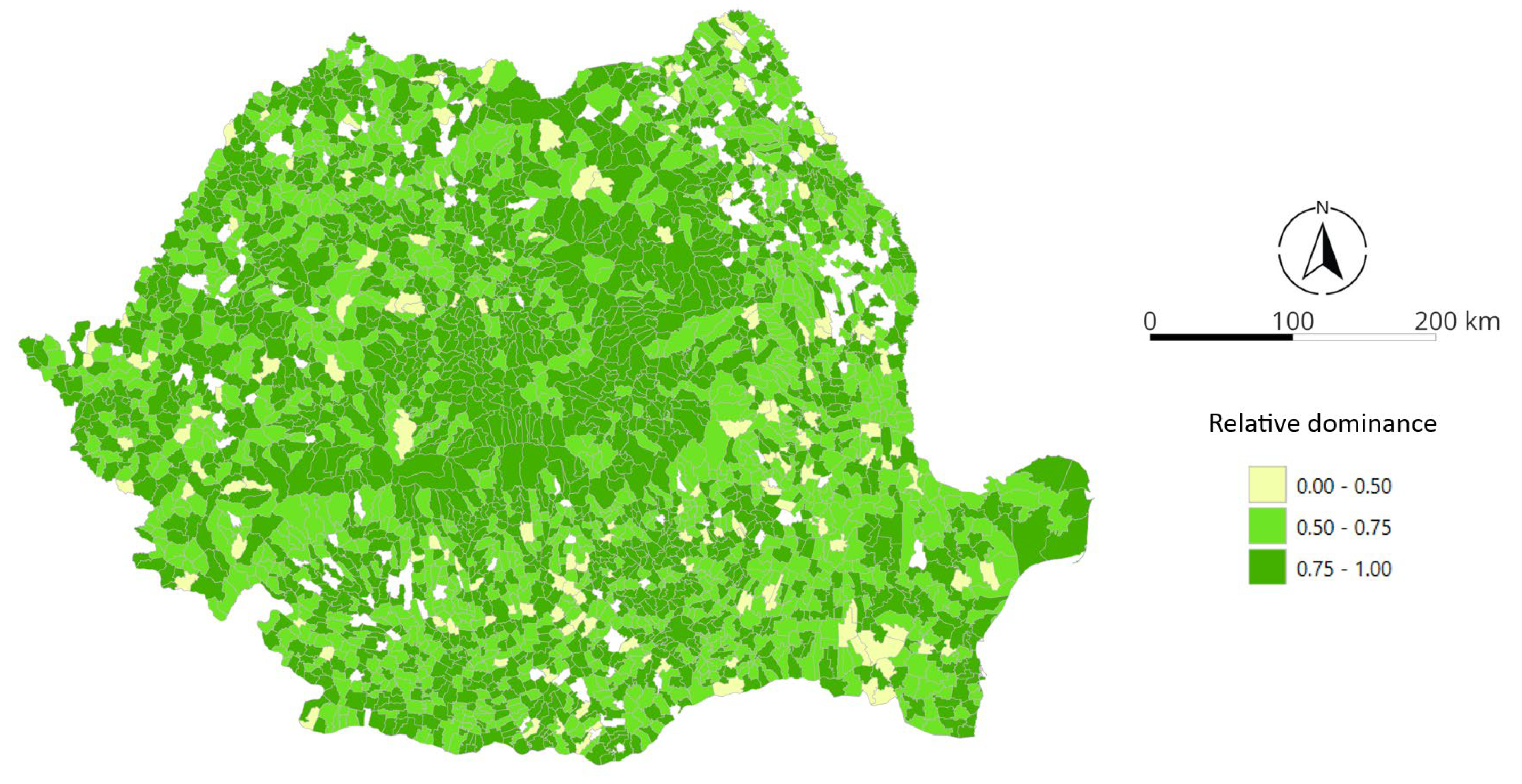
For the vast majority of the studied settlements, the aggregated built-up estimate is most influenced by the GHS single-source weight reducing parameter, which is the strongest factor in 2704 of 2974 settlements. The MSBF weight-reducing factor became dominant in relatively few places (169 cases), and OSM weight even less often (101 cases). Consequently, in areas lacking all three sources, the built-up estimate is particularly sensitive to how the GHS-based single-source contribution is scaled (Figure 11).
Regarding factor behavior, the OSM weight has a relatively small impact but is stable and linear, making its effect predictable and low-risk. By contrast, GHS and MSBF reducing factors are almost universally nonlinear, indicating strong context dependence and disproportionate influence via interactions or nonlinear responses. Small parameter changes can sometimes produce large shifts, and sometimes only marginal effects, leading to local instability and increased uncertainty. Dominance clarity also varies: the dominant factor’s relative contribution is typically higher than 0.5, so a single factor usually dominates variability. However, in some settlements the effects are more distributed, and output sensitivity is correspondingly less clear (Figure 12).
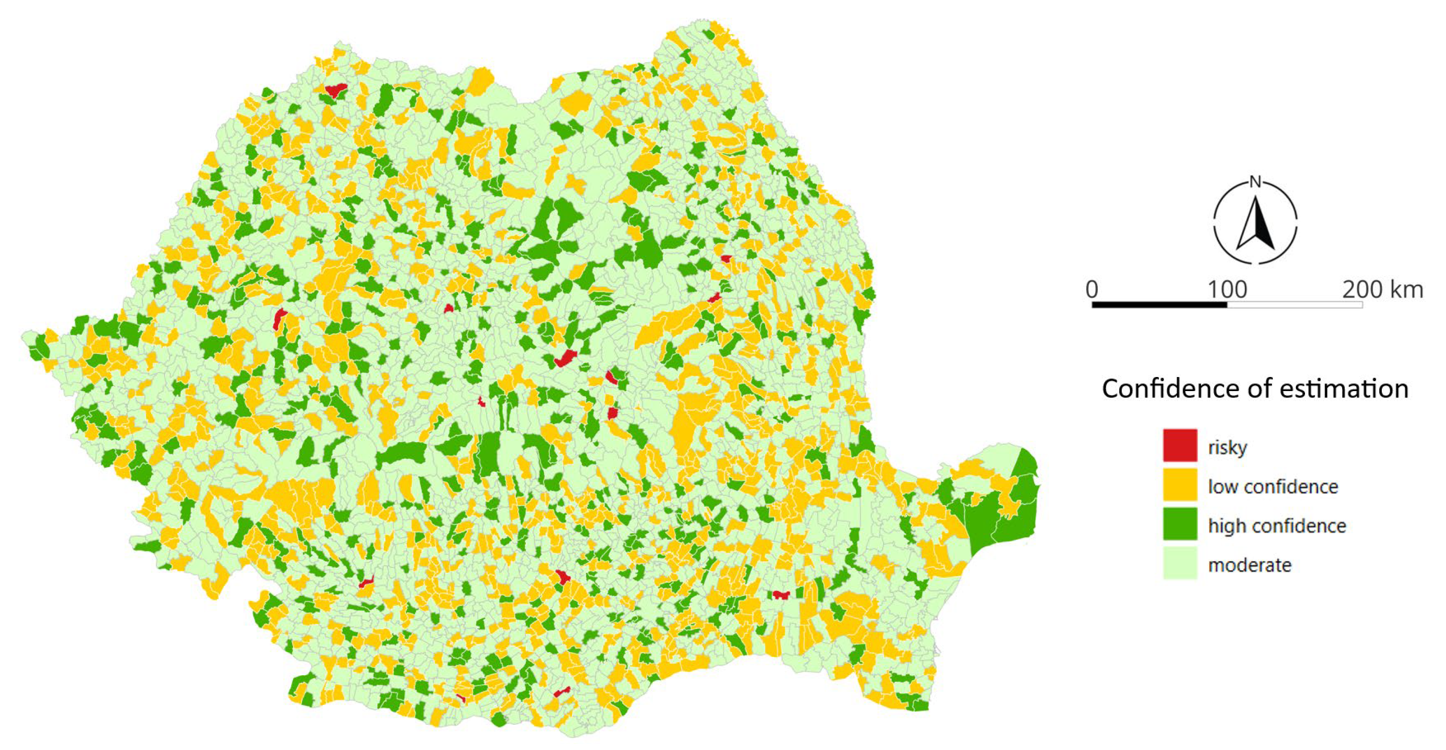
When not all three data sources indicate built-up area, the GHS weight-reducing factor is typically the main driver; however, its nonlinear behavior makes local estimates less robust, warranting cautious interpretation or finer, targeted decomposition in those areas. As a stable secondary component, the OSM weight poses less risk, while the MSBF reduction factor dominates less frequently but also exhibits nonlinear responses when it does. Particularly concerning are settlements where the dominant factor’s relative contribution is low yet the nonlinearity indicator is high: in such cases, output reliability decreases due to the combined effects of the inputs, and further targeted analysis or validation is advisable (Figure 13).
To assess robustness, we performed a bounded sensitivity analysis using three OSM fallback weights (0.80, 0.90, 1.00) and four single-source reduction factors for GHS/MSBF (2, 3, 4, 5), for a total of 12 runs. The OSM weight showed the smallest influence (consistent with the rarity of pixels where OSM is present and both GHS and MSBF are absent), whereas increasing the GHS/MSBF reductions decreased built-up area monotonically, reflecting the more common case of remote-sensing-only indications (Figure 14). The coefficient of variation across simulations was smaller than 1.5% in villages, smaller than 2% in cities, and at most 2.73% in municipalities, indicating limited sensitivity overall. Relative to the baseline (OSM = 0.95; reductions = 3), changing the OSM weight produced less than 0.5% shifts for the vast majority of settlements (Figure 15); setting the reduction factor to 2 yielded less than 1% change for 40% of settlements and less than 5% for a further 50%; and setting the reduction factor to 4 kept 60% of settlements with a less than 1% change.
A key constraint of the research is that zero cells in OSM—which may reflect unmapped areas rather than true absence—do not contribute to weight estimation. Consequently, in settlements where OSM coverage is particularly incomplete, the ensemble’s accuracy may be reduced. To reduce OSM zero ambiguity, further studies should combine time-stamped OSM edit history with auxiliary evidence (high-resolution imagery, night-time lights, population grids, land-cover, municipal registries) and fit a logistic model to estimate the probability of true vs. mapping zeros; these probabilities could then be propagated into ETC/CTC to obtain more robust weights. Another methodological limitation is the temporal heterogeneity of the data sources, collected at different times and with varying recency across settlements, complicating temporal comparability. Although ETC/CTC partially mitigates these differences, the effect cannot be fully eliminated. In addition, the absence of national reference data prevents direct validation, which makes objective evaluation of the results more challenging. In further studies, temporal heterogeneity could be reduced by defining a common reference window and using source versions that fall within it whenever possible. In addition, a lag penalty can be applied to sources outside that window—systematically down-weighting layers the farther their timestamps are from the reference period—so that temporally mismatched data exert less influence on the ensemble.
These results open promising avenues for refining and applying built-up coverage datasets. One direction is to compare the ensemble with machine-learning-derived built-up models. Integrating or benchmarking outputs from multiple ML algorithms could help characterize the behavior of each source more precisely and, in turn, improve the ensemble’s predictive ability and stability. A more complex, multidisciplinary program along these lines would further highlight the strengths of our methodology and expand its practical use in built-environment monitoring and spatial planning. A possible next step to better quantify result uncertainty—if multi-epoch inputs become available—would be to assemble a reference window and apply a lag-penalty scheme to explicitly quantify temporal drift. The ensemble could then be re-run across epochs to map drift sensitivity and provide settlement-level diagnostics that flag locations where temporal mismatch most affects the results.
The resulting 10 m ensemble is directly usable for Romanian public-sector workflows: in seismic risk (Vrancea corridor and major cities) to map exposed built-up areas and prioritize reinforcement; in heritage protection to screen buffers around listed assets and historic fabrics; in flood risk along the Danube, Siret, and Prut rivers to intersect built-up density and recent growth with floodplains and produce confidence-graded exposure maps; in landslide-prone Carpathian areas and wildfire belts to rank hotspots where expansion meets hazard; in urban heat and climate-adaptation planning to identify heat-vulnerable districts and target greening; in transport and utilities planning to validate service coverage and detect underserved or rapidly growing fringes; and in Black Sea coastal management to monitor built-up encroachment near erosion-sensitive shorelines. In every case the workflow is the same: standardize the CRS, clip to the area of interest, aggregate the 10 m raster to blocks or census units, and join available attributes. Then, use the ensemble weights and cell-level confidence intervals to estimate exposure with its uncertainty and rank where to audit or invest first—areas with high exposure but low confidence. Because the pipeline is replicable, annual or semi-annual re-runs keep baselines current for hazard models, SDG/urban-services monitoring, and evidence-based policy.

5. Conclusions

The primary objective of this research was to integrate the three comprehensive and widely used building and built-up coverage datasets (OSM, MSBF, GHS) to produce a more complete, accurate, and reliable national surface for Romania. The methodological approach used in the study (TCA/ETC/CTC) is well-suited to combining multiple data sources in the absence of ground truth. We successfully applied this method, creating a model which delivers CTC-based BLUE weighting with quantified uncertainty. The computational and time resource requirements for producing the model are moderate. The full national run at 10 m resolution was completed on a standard workstation (Intel i7–class CPU, 16 GB RAM) in under four hours, with no GPU or cluster resources.
Because the built environment evolves over time, the model is designed to be updatable, ensuring that each refresh more closely reflects the current state of built-up areas. Under the GHSL 2023 data package, the 10 m GHS-BUILT-S was available only for the 2018 reference year, which was used here. As additional 10 m epochs are released, the ensemble can be re-run using the open pipeline and code on GitHub to integrate the new layers and automatically re-estimate the ETC/CTC scale factors and error variances, thereby refreshing the national built-up surface and enabling same-resolution temporal assessment.
Although the ensemble model—like any model—cannot fully reflect reality, especially because its input sources are updated asynchronously and at different intervals, it provides a novel and practical way to harmonize these sources, thereby improving both accuracy and timeliness. Developed for Romania, our findings have broader relevance for regions with similar settlement structures. In small or peri-urban settlements, OSM often carries less redundant error and gains weight; in municipalities, higher OSM–MSBF correlation reduces both and increases the GHS share, reflecting denser, more homogeneous fabrics. These patterns echo global disparities in building-data completeness and scaling needs, suggesting that region-specific weighting can improve exposure baselines elsewhere. From a resilience perspective, tighter population–built-up coupling in municipalities implies more predictable exposure, whereas smaller settlements show higher data-uncertainty, warranting targeted audits. Policy-wise, authorities should use ensemble weights as a data-quality layer to prioritize ground validation where weights are unstable, apply explicit scaling to GHS-like layers in dense cores, and update the ensembles regularly to keep hazard modeling and SDG planning current across different city types.

Supplementary Materials

The following supporting information can be downloaded at https://www.mdpi.com/article/10.3390/ijgi14110420/s1. Document S1: Case studies for partial validation of the results

Author Contributions

Conceptualization, Zsolt Magyari-Sáska and Ionel Haidu; methodology, Zsolt Magyari-Sáska and Ionel Haidu; software, Zsolt Magyari-Sáska; validation, Zsolt Magyari-Sáska and Ionel Haidu; formal analysis, Zsolt Magyari-Sáska and Ionel Haidu; investigation, Zsolt Magyari-Sáska; resources, Zsolt Magyari-Sáska; data curation, Zsolt Magyari-Sáska; writing—original draft preparation, Zsolt Magyari-Sáska and Ionel Haidu; writing—review and editing, Zsolt Magyari-Sáska and Ionel Haidu; visualization, Zsolt Magyari-Sáska; supervision, Zsolt Magyari-Sáska; project administration, Zsolt Magyari-Sáska. All authors have read and agreed to the published version of the manuscript.

Funding

This research received no external funding.

Data Availability Statement

All created data are available at Zenodo https://doi.org/10.5281/zenodo.16742094 (accessed on 8 October 2025). The R script generating data is available on GitHub https://github.com/zsmagyari/Romania_BuildingFootprint (accessed on 8 October 2025).

Conflicts of Interest

The authors declare no conflicts of interest.

Abbreviations

The following abbreviations are used in this manuscript:
BLUEBest Linear Unbiased Estimate
CTCCorrelated Triple Collocation
GERSGlobal Entity Reference System
ENSEnsemble model
ETCExtended Triple Collocation
GHSGlobal Human Settlement Layer Built-S
RNSORomanian National Statistical Office
LAULocal Administrative Units
MCDAMulti-Criteria Decision Analysis
MSBFMicrosoft Building Footprint
OSMOpenStreetMap
TCATriple Collocation Analysis

References

  1. de Arruda, H.F.; Reia, S.M.; Ruan, S.; Atwal, K.S.; Kavak, H.; Anderson, T.; Pfoser, D. An OpenStreetMap Derived Building Classification Dataset for the United States. Sci. Data 2024, 11, 1210. [Google Scholar] [CrossRef]
  2. Biljecki, F.; Chow, Y.S. Global Building Morphology Indicators. Comput. Environ. Urban Syst. 2022, 95, 101809. [Google Scholar] [CrossRef]
  3. Chamberlain, H.R.; Pollard, D.; Winters, A.; Renn, S.; Borkovska, O.; Musuka, C.A.; Membele, G.; Lazar, A.N.; Tatem, A.J. Assessing the Impact of Building Footprint Dataset Choice for Health Programme Planning: A Case Study of Indoor Residual Spraying (IRS) in Zambia. Int. J. Health Geogr. 2025, 24, 13. [Google Scholar] [CrossRef]
  4. Che, Y.; Li, X.; Liu, X.; Wang, Y.; Liao, W.; Zheng, X.; Zhang, X.; Xu, X.; Shi, Q.; Zhu, J.; et al. 3D-GloBFP: The First Global Three-Dimensional Building Footprint Dataset. Earth Syst. Sci. Data 2024, 16, 5357–5374. [Google Scholar] [CrossRef]
  5. Chamberlain, H.R.; Darin, E.; Adewole, W.A.; Jochem, W.C.; Lazar, A.N.; Tatem, A.J. Building Footprint Data for Countries in Africa: To What Extent Are Existing Data Products Comparable? Comput. Environ. Urban Syst. 2024, 110, 102104. [Google Scholar] [CrossRef]
  6. Boo, G.; Darin, E.; Leasure, D.R.; Dooley, C.A.; Chamberlain, H.R.; Lázár, A.N.; Tschirhart, K.; Sinai, C.; Hoff, N.A.; Fuller, T.; et al. High-Resolution Population Estimation Using Household Survey Data and Building Footprints. Nat. Commun. 2022, 13, 1330. [Google Scholar] [CrossRef] [PubMed]
  7. Lebakula, V.; Sims, K.; Reith, A.; Rose, A.; McKee, J.; Coleman, P.; Kaufman, J.; Urban, M.; Jochem, C.; Whitlock, C.; et al. LandScan Global 30 Arcsecond Annual Global Gridded Population Datasets from 2000 to 2022. Sci. Data 2025, 12, 495. [Google Scholar] [CrossRef]
  8. Herfort, B.; Lautenbach, S.; Porto De Albuquerque, J.; Anderson, J.; Zipf, A. A Spatio-Temporal Analysis Investigating Completeness and Inequalities of Global Urban Building Data in OpenStreetMap. Nat. Commun. 2023, 14, 3985. [Google Scholar] [CrossRef]
  9. Wiedmann, T.; Allen, C. City Footprints and SDGs Provide Untapped Potential for Assessing City Sustainability. Nat. Commun. 2021, 12, 3758. [Google Scholar] [CrossRef]
  10. De Bono, A.; Mora, M.G. A Global Exposure Model for Disaster Risk Assessment. Int. J. Disaster Risk Reduct. 2014, 10, 442–451. [Google Scholar] [CrossRef]
  11. Kazmi, H.; Fu, C.; Miller, C. Ten Questions Concerning Data-Driven Modelling and Forecasting of Operational Energy Demand at Building and Urban Scale. Build. Environ. 2023, 239, 110407. [Google Scholar] [CrossRef]
  12. Milojevic-Dupont, N.; Wagner, F.; Nachtigall, F.; Hu, J.; Brüser, G.B.; Zumwald, M.; Biljecki, F.; Heeren, N.; Kaack, L.H.; Pichler, P.-P.; et al. EUBUCCO v0.1: European Building Stock Characteristics in a Common and Open Database for 200+ Million Individual Buildings. Sci. Data 2023, 10, 147. [Google Scholar] [CrossRef]
  13. Gherheș, V.; Grecea, C.; Vilceanu, C.-B.; Herban, S.; Coman, C. Challenges in Systematic Property Registration in Romania: An Analytical Overview. Land 2025, 14, 1118. [Google Scholar] [CrossRef]
  14. Păunescu, V.; Kohli, D.; Iliescu, A.-I.; Nap, M.-E.; Șuba, E.-E.; Sălăgean, T. An Evaluation of the National Program of Systematic Land Registration in Romania Using the Fit for Purpose Spatial Framework Principles. Land 2022, 11, 1502. [Google Scholar] [CrossRef]
  15. Nistor, C.; Vîrghileanu, M.; Cârlan, I.; Mihai, B.-A.; Toma, L.; Olariu, B. Remote Sensing-Based Analysis of Urban Landscape Change in the City of Bucharest, Romania. Remote Sens. 2021, 13, 2323. [Google Scholar] [CrossRef]
  16. Zhu, X.X.; Chen, S.; Zhang, F.; Shi, Y.; Wang, Y. GlobalBuildingAtlas: An Open Global and Complete Dataset of Building Polygons, Heights and LoD1 3D Models. arXiv 2025, arXiv:10.48550/arXiv.2506.04106. [Google Scholar]
  17. Albulescu, A.-C.; Grozavu, A.; Larion, D.; Burghiu, G. Assessing the Earthquake Systemic Vulnerability of the Urban Centres in the South-East Region of Romania. The Tale of Galați and Brăila Cities, Romania. Geomat. Nat. Hazards Risk 2022, 13, 1106–1133. [Google Scholar] [CrossRef]
  18. Paunescu, M.; Luca, O.; Stanescu, A.A.; Gaman, F. Digital Mapping and Resilience Indicators, as Pillars of Bucharest’s Seismic Resilience Strategy. Infrastructures 2025, 10, 39. [Google Scholar] [CrossRef]
  19. Albano, R.; Samela, C.; Crăciun, I.; Manfreda, S.; Adamowski, J.; Sole, A.; Sivertun, Å.; Ozunu, A. Large Scale Flood Risk Mapping in Data Scarce Environments: An Application for Romania. Water 2020, 12, 1834. [Google Scholar] [CrossRef]
  20. Ţîncu, R.; Zêzere, J.L.; Lazar, G. Identification of Elements Exposed to Flood Hazard in a Section of Trotus River, Romania. Geomat. Nat. Hazards Risk 2018, 9, 950–969. [Google Scholar] [CrossRef]
  21. Biljecki, F.; Chow, Y.S.; Lee, K. Quality of Crowdsourced Geospatial Building Information: A Global Assessment of OpenStreetMap Attributes. Build. Environ. 2023, 237, 110295. [Google Scholar] [CrossRef]
  22. Ullah, T.; Lautenbach, S.; Herfort, B.; Reinmuth, M.; Schorlemmer, D. Assessing Completeness of OpenStreetMap Building Footprints Using MapSwipe. ISPRS Int. J. Geoinf. 2023, 12, 143. [Google Scholar] [CrossRef]
  23. Yang, A.; Fan, H.; Jia, Q.; Ma, M.; Zhong, Z.; Li, J.; Jing, N. How Do Contributions of Organizations Impact Data Inequality in OpenStreetMap? Comput. Environ. Urban Syst. 2024, 109, 102077. [Google Scholar] [CrossRef]
  24. Florio, P.; Giovando, C.; Goch, K.; Pesaresi, M.; Politis, P.; Martinez, A. Towards a Pan-EU Building Footprint Map Based on The Hierarchical Conflation of Open Datasets: The Digital Building Stock Model—DBSM. Int. Arch. Photogramm. Remote Sens. Spat. Inf. Sci. 2023, 48, 47–52. [Google Scholar] [CrossRef]
  25. Gonzales, J.J. Building-Level Comparison of Microsoft and Google Open Building Footprints Datasets (Short Paper). In Proceedings of the Leibniz International Proceedings in Informatics (LIPIcs), International Conference on Geographic Information Science (GIScience), Leeds, UK, 12–15 September 2023; Volume 277, pp. 35:1–35:6. [Google Scholar] [CrossRef]
  26. Litwintschik, M. Microsoft’s 1.4 Billion Global ML Building Footprints. 2024. Available online: https://tech.marksblogg.com/microsofts-global-ml-building-footprints.html (accessed on 8 October 2025).
  27. Pesaresi, M. GHS-BUILT-S R2023A—GHS Built-Up Surface Grid, Derived from Sentinel2 Composite and Landsat, Multitemporal (1975–2030); European Commission: Brussels, Belgium, 2023. [Google Scholar]
  28. Pesaresi, M.; Schiavina, M.; Politis, P.; Freire, S.; Krasnodębska, K.; Uhl, J.H.; Carioli, A.; Corbane, C.; Dijkstra, L.; Florio, P.; et al. Advances on the Global Human Settlement Layer by Joint Assessment of Earth Observation and Population Survey Data. Int. J. Digit. Earth 2024, 17, 2390454. [Google Scholar] [CrossRef]
  29. Liu, F.; Wang, S.; Xu, Y.; Ying, Q.; Yang, F.; Qin, Y. Accuracy Assessment of Global Human Settlement Layer (GHSL) Built-up Products over China. PLoS ONE 2020, 15, e0233164. [Google Scholar] [CrossRef]
  30. Liu, Z.; Huang, S.; Fang, C.; Guan, L.; Liu, M. Global Urban and Rural Settlement Dataset from 2000 to 2020. Sci. Data 2024, 11, 1359. [Google Scholar] [CrossRef]
  31. Ning, S.; Cheng, Y.; Zhou, Y.; Wang, J.; Zhang, Y.; Jin, J.; Thapa, B.R. Bayesian Model Averaging for Satellite Precipitation Data Fusion: From Accuracy Estimation to Runoff Simulation. Remote Sens. 2025, 17, 1154. [Google Scholar] [CrossRef]
  32. Khan, A.A.; Chaudhari, O.; Chandra, R. A Review of Ensemble Learning and Data Augmentation Models for Class Imbalanced Problems: Combination, Implementation and Evaluation. Expert Syst. Appl. 2024, 244, 122778. [Google Scholar] [CrossRef]
  33. Xiao, F.; Wen, J.; Pedrycz, W.; Aritsugi, M. Complex Evidence Theory for Multisource Data Fusion. Chin. J. Inf. Fusion 2024, 1, 134–159. [Google Scholar] [CrossRef]
  34. Khan, M.N.; Anwar, S. Paradox Elimination in Dempster–Shafer Combination Rule with Novel Entropy Function: Application in Decision-Level Multi-Sensor Fusion. Sensors 2019, 19, 4810. [Google Scholar] [CrossRef]
  35. Seoni, S.; Jahmunah, V.; Salvi, M.; Barua, P.D.; Molinari, F.; Acharya, U.R. Application of Uncertainty Quantification to Artificial Intelligence in Healthcare: A Review of Last Decade (2013–2023). Comput. Biol. Med. 2023, 165, 107441. [Google Scholar] [CrossRef] [PubMed]
  36. Greene, R.; Devillers, R.; Luther, J.E.; Eddy, B.G. GIS-Based Multiple-Criteria Decision Analysis. Geogr. Compass 2011, 5, 412–432. [Google Scholar] [CrossRef]
  37. Stoffelen, A. Toward the True Near-Surface Wind Speed: Error Modeling and Calibration Using Triple Collocation. J. Geophys. Res. Ocean. 1998, 103, 7755–7766. [Google Scholar] [CrossRef]
  38. Yilmaz, M.T.; Crow, W.T. Evaluation of Assumptions in Soil Moisture Triple Collocation Analysis. J. Hydrometeorol. 2014, 15, 1293–1302. [Google Scholar] [CrossRef]
  39. Gruber, A.; Su, C.-H.; Zwieback, S.; Crow, W.; Dorigo, W.; Wagner, W. Recent Advances in (Soil Moisture) Triple Collocation Analysis. Int. J. Appl. Earth Obs. Geoinf. 2016, 45, 200–211. [Google Scholar] [CrossRef]
  40. Xie, Q.; Jia, L.; Menenti, M.; Hu, G. Global Soil Moisture Data Fusion by Triple Collocation Analysis from 2011 to 2018. Sci. Data 2022, 9, 687. [Google Scholar] [CrossRef]
  41. Pataki, A.; Bertalan, L.; Pásztor, L.; Nagy, L.A.; Abriha, D.; Liang, S.; Singh, S.K.; Szabó, S. Soil Moisture Satellite Data Under Scrutiny: Assessing Accuracy Through Environmental Proxies and Extended Triple Collocation Analysis. Earth Syst. Environ. 2025, 9, 801–824. [Google Scholar] [CrossRef]
  42. Li, Y.; Lu, J.; Huang, P.; Chen, X.; Jin, H.; Zhu, Q.; Luo, H. Triple Collocation-Based Model Error Estimation of VIC-Simulated Soil Moisture at Spatial and Temporal Scales in the Continental United States in 2010–2020. Water 2024, 16, 3049. [Google Scholar] [CrossRef]
  43. Chen, P.; Huang, H.; Shi, W.; Chen, R. A Reference-Free Method for the Thematic Accuracy Estimation of Global Land Cover Products Based on the Triple Collocation Approach. Remote Sens. 2023, 15, 2255. [Google Scholar] [CrossRef]
  44. Li, T.; Wang, Y.; Wang, B.; Liu, K.; Chen, X.; Sun, R. Evaluation and Fusion of Multi-Source Sea Ice Thickness Products with Limited in-Situ Observations. Front. Mar. Sci. 2024, 11, 1464391. [Google Scholar] [CrossRef]
  45. Li, X.; Zhang, W.; Vermeulen, A.; Dong, J.; Duan, Z. Triple Collocation-Based Merging of Multi-Source Gridded Evapotranspiration Data in the Nordic Region. Agric. For. Meteorol. 2023, 335, 109451. [Google Scholar] [CrossRef]
  46. Chen, C.; He, M.; Chen, Q.; Zhang, J.; Li, Z.; Wang, Z.; Duan, Z. Triple Collocation-Based Error Estimation and Data Fusion of Global Gridded Precipitation Products over the Yangtze River Basin. J. Hydrol. 2022, 605, 127307. [Google Scholar] [CrossRef]
  47. Dong, J.; Lei, F.; Wei, L. Triple Collocation Based Multi-Source Precipitation Merging. Front. Water 2020, 2, 1–9. [Google Scholar] [CrossRef]
  48. Wei, L.; Jiang, S.; Dong, J.; Ren, L.; Yong, B.; Yang, B.; Li, X.; Duan, Z. A Combined Extended Triple Collocation and Cumulative Distribution Function Merging Framework for Improved Daily Precipitation Estimates over Mainland China. J. Hydrol. 2024, 641, 131757. [Google Scholar] [CrossRef]
  49. McColl, K.A.; Vogelzang, J.; Konings, A.G.; Entekhabi, D.; Piles, M.; Stoffelen, A. Extended Triple Collocation: Estimating Errors and Correlation Coefficients with Respect to an Unknown Target. Geophys. Res. Lett. 2014, 41, 6229–6236. [Google Scholar] [CrossRef]
  50. González-Gambau, V.; Turiel, A.; González-Haro, C.; Martínez, J.; Olmedo, E.; Oliva, R.; Martín-Neira, M. Triple Collocation Analysis for Two Error-Correlated Datasets: Application to L-Band Brightness Temperatures over Land. Remote Sens. 2020, 12, 3381. [Google Scholar] [CrossRef]
  51. Morris, M.D. Factorial Sampling Plans for Preliminary Computational Experiments. Technometrics 1991, 33, 161. [Google Scholar] [CrossRef]
  52. Gupta, D.; Dhanya, C.T. Influence of Spatial Heterogeneity in Error Characterization Using Triple Collocation; Copernicus GmbH: Göttingen, Germany, 2025. [Google Scholar]
  53. Ford, T.W.; Quiring, S.M.; Zhao, C.; Leasor, Z.T.; Landry, C. Triple Collocation Evaluation of In Situ Soil Moisture Observations from 1200+ Stations as Part of the U.S. National Soil Moisture Network. J. Hydrometeorol. 2020, 21, 2537–2549. [Google Scholar] [CrossRef]
  54. Yin, G.; Park, J. The Use of Triple Collocation Approach to Merge Satellite- and Model-Based Terrestrial Water Storage for Flood Potential Analysis. J. Hydrol. 2021, 603, 127197. [Google Scholar] [CrossRef]
  55. Mohammedshum, A.A.; Maathuis, B.H.P.; Mannaerts, C.M.; Teka, D. Using a Triple Sensor Collocation Approach to Evaluate Small-Holder Irrigation Scheme Performances in Northern Ethiopia. Water 2024, 16, 2638. [Google Scholar] [CrossRef]
  56. Uhl, J.H.; Leyk, S. Spatially Explicit Accuracy Assessment of Deep Learning-Based, Fine-Resolution Built-up Land Data in the United States. Int. J. Appl. Earth Obs. Geoinf. 2023, 123, 103469. [Google Scholar] [CrossRef]
  57. Heris, M.P.; Foks, N.L.; Bagstad, K.J.; Troy, A.; Ancona, Z.H. A Rasterized Building Footprint Dataset for the United States. Sci. Data 2020, 7, 207. [Google Scholar] [CrossRef]
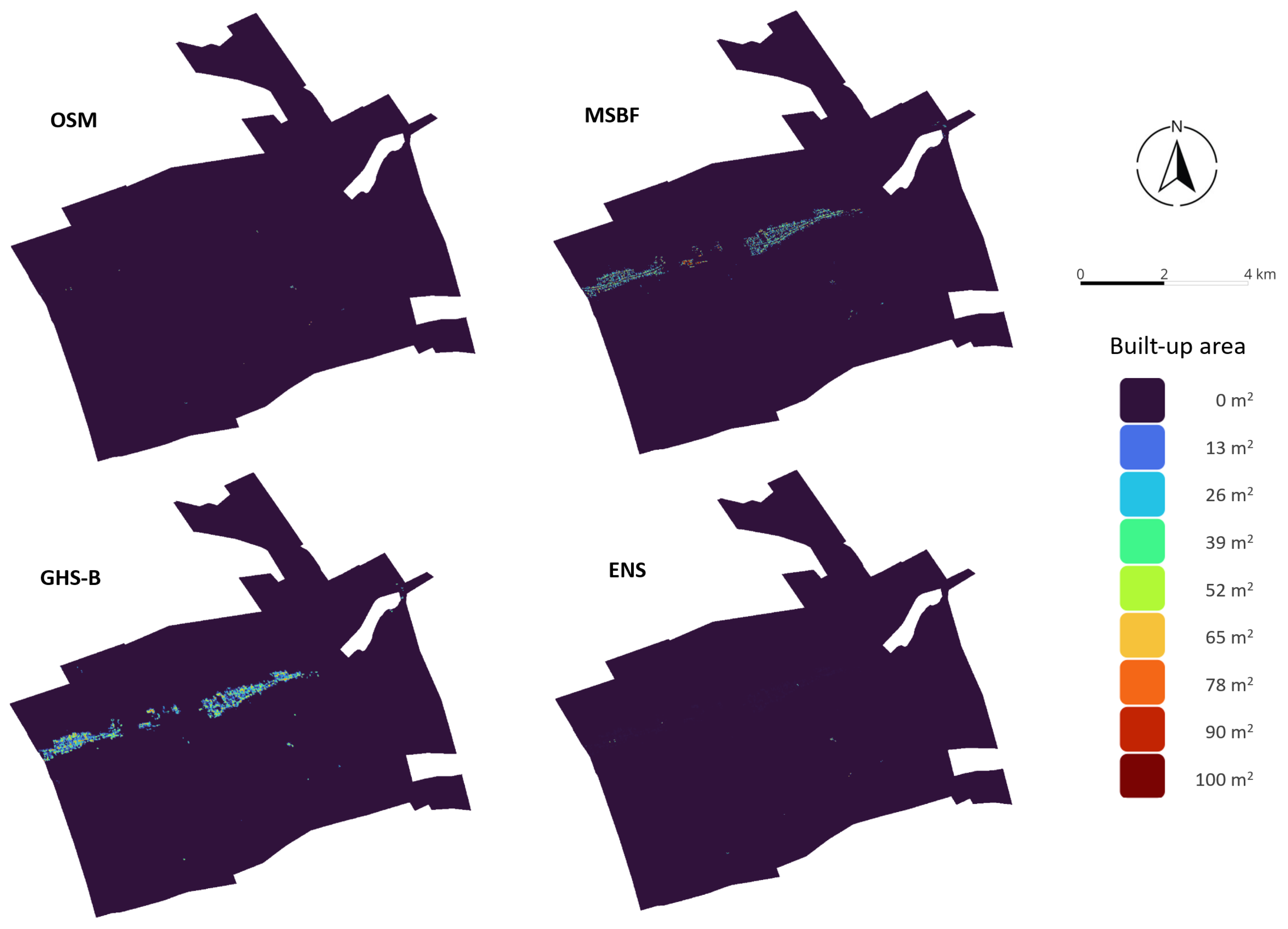
Figure 1. Influence of the misinterpreted OSM zero values on the resulting ensemble model (Nasturelu settlement—lat: 43.67°, lon: 25.47°).
Ijgi 14 00420 g001
Figure 2. Built-up area calculated at settlement level for OSM, MSBF, GHS, and the resulting ensemble model (ENS).
Ijgi 14 00420 g002
Figure 3. Gheorgheni case study: improvements in ensemble model based on the weighted combination of data sources—lat: 46.72°, lon: 25.60°.
Ijgi 14 00420 g003
Figure 4. Confidence interval width for the ensemble model—case of Gheorgheni, lat: 46.72°, lon: 25.60°.
Ijgi 14 00420 g004
Figure 5. Roads that are not visible in GHS but are captured in the ENS due to OSM and MSBF (case of Arad city—lat: 46.18°, lon: 21.30°).
Ijgi 14 00420 g005
Figure 6. Pearson correlation between population and built-up area of the ensemble model.
Ijgi 14 00420 g006
Figure 7. Ratio of built-up areas at the settlement level of the ENS model compared to the GHS value.
Ijgi 14 00420 g007
Figure 8. Built-up area ratio of different data sources against the ensemble model (AC) and settlements with most balanced contribution to the ensemble model (D).
Ijgi 14 00420 g008
Figure 9. Weight characteristics for the three data sources on settlement categories.
Ijgi 14 00420 g009
Figure 10. Correlation by settlement type between data sources weight and built-up area characteristics (floor area from RNSO, ensemble-model-generated area, built-up density ratio).
Ijgi 14 00420 g010
Figure 11. Dominant factor spatial distribution.
Ijgi 14 00420 g011
Figure 12. Relative strength of the dominant factor.
Ijgi 14 00420 g012
Figure 13. Ensemble model confidence based on factor’s sensitivity analysis.
Ijgi 14 00420 g013
Figure 14. Mean built-up area across settlements under alternative parameter settings.
Ijgi 14 00420 g014
Figure 15. Built-up area changes under alternative OSM fallback weights relative to the 0.95 baseline.
Ijgi 14 00420 g015
Table 1. Data source and format for the used datasets.
NameData SourceRelease DateData FormatResolution
OSMhttps://download.geofabrik.de/europe/romania.html18 June 2025vector → raster10 m
MSBFhttps://minedbuildings.z5.web.core.windows.net/global-buildings/dataset-links.csv2 January 2025vector → raster10 m
GHShttps://human-settlement.emergency.copernicus.eu/download.php2018raster10 m
All datasets were downloaded on 19 June 2025.
Disclaimer/Publisher’s Note: The statements, opinions and data contained in all publications are solely those of the individual author(s) and contributor(s) and not of MDPI and/or the editor(s). MDPI and/or the editor(s) disclaim responsibility for any injury to people or property resulting from any ideas, methods, instructions or products referred to in the content.