Massively Parallel Lagrangian Relaxation Algorithm for Solving Large-Scale Spatial Optimization Problems Using GPGPU

Abstract

Lagrangian Relaxation (LR) is an effective method for solving spatial optimization problems in geospatial analysis and GIS. Among others, it has been used to solve the classic p-median problem that served as a unified local model in GIS since the 1990s. Despite its efficiency, the LR algorithm has seen limited usage in practice and is not as widely used as off-the-shelf solvers such as OPL/CPLEX or GPLK. This is primarily because of the high cost of development, which includes (i) the cost of developing a full gradient descent algorithm for each optimization model with various tricks and modifications to improve the speed, (ii) the computational cost can be high for large problem instances, (iii) the need to test and choose from different relaxation schemes, and (iv) the need to derive and compute the gradients in a programming language. In this study, we aim to solve the first three issues by utilizing the computational power of GPGPU and existing facilities of modern deep learning (DL) frameworks such as PyTorch. Based on an analysis of the commonalities and differences between DL and general optimization, we adapt DL libraries for solving LR problems. As a result, we can choose from the many gradient descent strategies (known as “optimizers”) in DL libraries rather than reinventing them from scratch. Experiments show that implementing LR in DL libraries is not only feasible but also convenient. Gradient vectors are automatically tracked and computed. Furthermore, the computational power of GPGPU is automatically used to parallelize the optimization algorithm (a long-term difficulty in operations research). Experiments with the classic p-median problem show that we can solve much larger problem instances (of more than 15,000 nodes) optimally or nearly optimally using the GPU-based LR algorithm. Such capabilities allow for a more fine-grained analysis in GIS. Comparisons with the OPL solver and CPU version of the algorithm show that the GPU version achieves speedups of 104 and 12.5, respectively. The GPU utilization rate on an RTX 4090 GPU reaches 90%. We then conclude with a summary of the findings and remarks regarding future work.

1. Introduction

Spatial optimization is an integral part of Geographic Information Systems (GIS). It involves location decisions about various service and logistics systems in terms of the location of central facilities such as factories and warehouses, the routes of transit and package delivery systems, and the location and boundaries of areal features such as electoral districts. One of the motivations of inventing GIS is to support spatial decision making. A classic spatial optimization problem is the classic p-median problem [1,2]. Also known as the multi-facility Weber problem, it is an extension of the Weber problem, and is aimed at optimally locating a set of facilities to minimize the total service distance to a set of customer locations. The p-median problem is important not only because of its wide application in transportation, public facility layout, and natural resource management, but also because of its generality. Researchers have found [3,4,5] that various other spatial optimization problems can be posed as special cases of the p-median problem. This includes the classic Simple Plant Location problem [6], the Maximal Covering Location Problem [7], and the hub median location problem [4,8], among others. In the context of GIS, this means that one can implement one solver for the p-median problem and use it as a unified solver for all the aforementioned special case problems of the p-median. This approach, known as unified location modeling [5,9], has been adopted by mainstream GIS vendors since the 1990s.

One of the problems in the application of spatial optimization models is the solution speed. Many classic spatial optimization problems are difficult to solve using off-the-shelf solvers such as IBM ILOG CPLEX or GNU GLPK. Especially for large problem instances, it can take an excessively long time to find the optimal solution of a model. Theoretically, this is because the p-median problem and many other classic spatial optimization models are NP-hard [10]. In practice, many have opted to use fast heuristic algorithms (e.g., [11]’s interchange heuristic) to solve the p-median problem. But this approach has its own issues. Generally, heuristic algorithms cannot guarantee to find an optimal solution when they terminate. In fact, they cannot even tell how far the final solution is from the optimal solution. All that is known is that the operations in the algorithm (e.g., the interchange operation in [11]) have stopped to find any better solutions. There is no guarantee that a different algorithm cannot find a better solution.

A solution method that is both fast and optimal for the p-median problem is Lagrangian Relaxation (LR). The main idea of Lagrangian Relaxation (LR) is to transform the original optimization problem (p-median) into a simpler problem by relaxing some of its constraints and penalizing the amount of violation associated with the relaxed constraints (hence the name Lagrangian Relaxation). Then, a sequence of the relaxed problem is solved with improving objective function values and decreasing amounts of violations (which will eventually reach zero at optimality). Just like various heuristic algorithms, a well-designed LR algorithm is usually fast compared to conventional optimal solution methods, such as mathematical programming. This is due to the simplicity of the relaxed Lagrangian problem (if well chosen). Unlike heuristic methods, the LR algorithm is optimal in that it provides an optimality gap, indicating the distance between the current solution and the optimal solution. The optimality gap, when reduced to zero, provides a proof of optimality (similar to mathematical programming).

Despite their merits, LR-based algorithms are not as widely adopted in practical spatial analysis as other approaches such as mathematical programming or heuristic algorithms. Presumably, this is because of the high cost of development and the fact that they are very problem-specific. Specialized code has to be written from scratch for each new optimization problem, and this involves both theoretical derivation of the Lagrangian function and its gradient, as well as the implementation of a full gradient optimization process in a programming language.

The goal of this article is to ease the development of LR algorithms by exploiting the mature tool-chain of deep learning. The main insight is that general optimization and modern deep learning have much in common in their methodologies, and techniques may be transferable from one to the other. For example, there is a gradient descent process at the heart of most deep learning algorithms, in which gradients of model parameters are computed from the loss function and used to iteratively reduce the loss function value. Essentially, the same gradient descent process has long been used in the operations research literature to solve general optimization problems such as the p-median [12,13,14]. On the other hand, such gradient-based algorithms have seen significant development in the deep learning literature due to recent advancements in Artificial Intelligence. Most notably, deep learning applications needed the capability to handle very large datasets and parameter sets, and have necessitated the massive parallelization of gradient descent algorithms. GPGPUs with over 10,000 cores can be readily used in DL libraries to efficiently solve the gradient optimization problem. Additionally, a large number of gradient optimization algorithms have been developed, standardized, and accumulated in mainstream DL libraries, each representing a variant of the prototypical gradient descent process. Such generalized algorithms, called “optimizers”, can easily be reused interchangeably to solve different DL problems.

In this article, we demonstrate that the existing facilitates of deep learning can be adapted to solve optimization problems, such as the p-median. Specifically, we use PyTorch Lightning (2.5.0) to implement a p-median Lagrangian Relaxation algorithm that can be executed in massive parallelization with GPGPU. The benefit of this approach is threefold: (i) it has the potential to efficiently utilize many processors and solve the long-term difficulty with parallelizing algorithms for spatial optimization problems. (ii) it allows much larger problem instances to be solved optimally or near optimally in a reasonable amount of time. (iii) basing our algorithm on the de facto deep learning frameworks reduces the development cost of LR algorithms, as we may reuse the stock optimizers therein and avoid reinventing the wheel. The auto-gradient computation in DL libraries also makes it possible to automatically compute the needed gradient vectors with massive parallelization. To our best knowledge, the massively parallel Lagrangian Relaxation method (with automatic gradient computation) is new, and no such algorithms have been presented in the literature.

In the rest of the article, we discuss the background of Lagrangian Relaxation, gradient descent algorithm, and its link to DL-based algorithms in the next section. Then, we introduce our p-median LR algorithm and demonstrate the necessary adaptations of the DL library for this algorithm. The experiment section presents the computational results, which demonstrate that we can solve much larger problem instances (of up to 15,000 nodes) optimally or nearly optimally using the GPU-based Lagrangian Relaxation algorithm. Comparisons with the OPL/CPLEX solver and CPU version of the algorithm show that the GPU-based LR algorithm achieves a speedup of approximately 100 over OPL/CPLEX and a speedup of 12 over the CPU version, respectively. The experiments also indicate that the algorithm can take full advantage of the computing power of GPU and the GPU utilization rate on a NVIDIA RTX 4090 GPU is approximately 90%.

2. Background

In this section, we review the background of Lagrangian Relaxation, the p-median problem, and deep learning algorithms with a focus on the optimization methodology. We review the common features and differences between DL and the general optimization methods. We then zoom in on the specific LR algorithm for the classic p-median problem.

2.1. Deep Learning and General Optimization

To understand the use of Deep Learning tools for general optimization, we first review the status quo and the basic format of the original deep learning problem. There are many variants of the deep learning problem, ranging from simple fully connected networks to the Convolutional Neural Network (CNN) [15], to generative AI networks [16]. It is not in the scope of this article to conduct a comprehensive review of all neural networks. Instead, we use the CNN and its descendants (widely used in the remote sensing literature) as a prototypical example to demonstrate the main features of deep learning and neural networks nowadays.

In its most basic form, the DL process takes as input a training dataset with labels and outputs a computed label for any new data of similar form (prediction). Roughly speaking, the training process establishes a model of the link between the input data and the known labels via an optimization process, which is then applied in the prediction stage to generate new labels. This optimization phase is what is of interest to general discrete optimization, and therefore will be discussed in greater detail.

From the perspective of optimization, the loss function is the objective function that we want to minimize. In deep learning, the loss function is typically a measure of the difference between the predicted output and the true output (i.e., the ground truth). It is possible to change or minimize the loss function because the predicted output is defined in terms of the parameters in the many layers of the neural network. The values of these parameters are unknown and are initialized randomly at the beginning. Such freedom in the parameter space allows room for improvement of the loss function. In case of the CNN and its descendant UNet, the parameters in the NN represent weight values used in convolutional kernels, which are essentially the same as the kernel parameters used in feature detectors (e.g., edge detectors) in traditional image processing. While kernel parameters in edge detectors are pre-specified by the human expert, they are left as unknowns and determined by the minimization of the loss function.

The core of the minimization process is the gradient descent algorithm. The algorithm is a simple iterative process that updates the model parameters in the direction of the negative gradient of the loss function. This direction is, by definition, the direction in which the loss function decreases the most. When the loss function is not differentiable, the so-called sub-gradient is used instead. When there is no ambiguity, we use the terms “gradient” and “sub-gradient” interchangeably in the rest of this article.

Figure 1 presents the diagram of the training process in a typical deep learning workflow. The Dataset module is responsible for loading and converting the training dataset into a form that is suitable for computing the loss function. This includes, e.g., slicing a remote sensing image into small tiles of patches that fit well in GPU memory. The training_step is responsible for computing the actual value of the loss function based on the layers of a NN and the weight values therein. The Optimizer implements the gradient descent algorithm. It is noteworthy that in many DL applications (e.g., remote sensing, LLM), the training datasets are quite large, and the associated weight values and their gradients may not fit into the memory. This is why the training process consists of multiple iterations as shown in Figure 1. Each iteration consumes a small subset (called a “minibatch”) of the training data to update the model parameters.

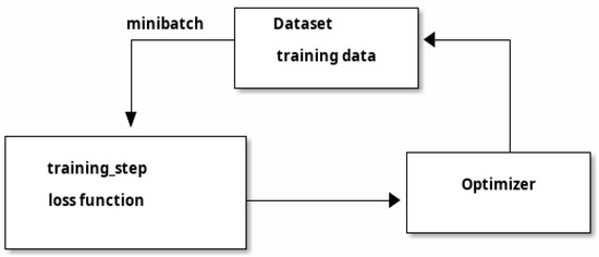
Figure 1. Components of training in a typical deep learning workflow.

A naive implementation of gradient descent may not work well. For example, the step size (or “learning rate”) at which we change a parameter in gradient descent is of paramount importance. If this value is too large, the gradient descent process may not converge at all (i.e., It may oscillate); if it is too small, the descent towards optimal values may be too slow. Different strategies are often used to control the descent process based on factors, such as the historical speed and inertial. State-of-the-art DL libraries provide different implementations of these strategies, and package them as different “Optimizers” as shown in Figure 1.

So far, this section presents a concise overview of the training process from the perspective of optimization, hiding many technical details. What is interesting is that the same workflow in Figure 1 can be applied to seemingly very different optimization problems such as the p-median, as will be discussed in the next subsection.

2.2. Gradient Descent for the Lagrangian Optimization

Having discussed how the training step and the optimizers, etc., work in DL, a natural question is whether this tool-chain applies to general optimization problems such as the p-median problem. The answer is yes. In this subsection, we discuss the characteristics of the p-median problem, the concept of relaxation and dual problems, and why the relaxed problems are actually easier to work with in a training workflow.

In neural networks such as CNN or UNet, the gradients of the loss function with respect to the model are computed using backpropagation. The model consists of a large number of interconnected simple functions, such as the weighted sum, ReLU, and other activation functions, so that the entire NN forms an explicit function from the input of the NN to its output labels. Even though such functions are quite large in terms of the number of coefficients or parameters, the gradients of the final loss function can be clearly computed using the chain rule in calculus. In fact, modern DL libraries support effective gradient computation using massive parallel processing in GPGPU and can derive the gradients of model parameters via automatic differentiation of the explicit function.

If one attempts to apply the same principles to solving the p-median problem, a natural question is: what is the gradient of the p-median problem? The p-median problem, first defined by [1,2], is aimed at locating $p$ facilities among a set $J$ of candidate sites so that the population weighted service distance to a set of customers $I$ is minimized. A classic formulation [17] of the p-median problem in integer linear programming is as follows:

$a_i$ is the amount of population at $i\in I$, and $d_{ij}$ is the distance between locations $i$ and $j$.

The decision variables for optimization are:

$$x_{ij}=1,\mathrm{if} \mathrm{customer} i \mathrm{is} \mathrm{served} \mathrm{by} j\in J, \mathrm{or} 0 \mathrm{otherwise}$$

(1)

$$y_j=1,\mathrm{if} \mathrm{there} \mathrm{is} \mathrm{an} \mathrm{open} \mathrm{facility} \mathrm{at} \mathrm{candidate} \mathrm{site} j\in J, 0 \mathrm{otherwise}$$

(2)

The optimization is to:

$$\mathrm{minimize}\sum _{i\in I,j\in J}{a}_i\cdot d_{ij}\cdot x_{ij}$$

(3)

Subject To:

$$\sum _{j\in J}{x}_{ij}=1,\forall i\in I$$

(4)

$$\sum _{j\in J}{y}_j\le p$$

(5)

$$x_{ij}\le y_j,\forall i\in I,j\in J$$

(6)

In above, the objective function (3) is used to minimize the total distance $d_{ij}$ for each customer’s location (weighted by its population $a_i$). Equations (4) and (6) are constraints stating that a customer $i$ can be assigned to at most one open facility $j$. Equation (5) states that no more than $p$ candidate sites can be selected as facilities. Equations (1) and (2) define the assignment variable $x_{ij}$ and location variable $y_j$ respectively.

With this definition in mind, a natural problem in computing the gradient of the p-median problem is that the function from problem data ($a,d$) to the model output (the objective function 3) is not free. In other words, the model is not a simple function of the decision variables (the equivalence of model parameters in DL). Rather, it is a summation function plus a set of side constraints ((4) through (5)) that the objective function must satisfy. Therefore, one cannot naively apply the chain rule or backpropagation to the objective function, since the real relationship between the unknown variables and the model output is an implicit function defined by both the objective function and the constraint set.

A good solution to the gradient definition problem is to use the Lagrangian relaxation. The essence of this method is that we can “dualize” the original optimization problem (p-median) and turn the implicit function between the model input and output into an explicit function. As discussed in the next section, we relax some of the constraints to obtain a simpler problem (the “dual” problem). In the dual problem, violations of relaxed constraints are allowed but penalized. The dual problem is called a dual because it is always super-optimal (i.e., better than the optimal solution). The key feature of a (good) Lagrangian Relaxation scheme is that the dual problem should be simple enough and at the same time have good convergence behavior. In particular, the dual problem should be simple enough to be described by a simple and explicit program similar to neural networks in deep learning.

The dual problem in Lagrangian Relaxation is not only simpler for gradient computation, but also gives rise to better termination criteria. In particular, the objective function values for the dual problem and the original problem (known as the “primal” problem) always differ when the solution is not optimal. On such occasions, the dual object is better than the optimal objective value (super-optimal) and therefore infeasible, while the primal solution is always sub-optimal and feasible. The difference between the dual and primal objective values is known as the optimality gap, and indicates how far the optimization process is from reaching an optimal solution. Then, a natural termination criterion terminates the optimization when the optimality gap is zero or close enough to zero. In comparison, in a typical training step of a deep learning algorithm, there is no knowledge of whether an optimal solution is reached or how close it is, and one has to rely on heuristic termination criteria, such as terminating the algorithm if the objective value does not change in a given number of iterations.

An important issue for the gradient optimization is the choice on the speed of gradient descent. That is, how fast should one move the parameters along the gradient direction? In its most basic form, the model parameters $x$ are updated by subtracting the gradient $\theta$ multiplied with a constant:

$$x_{t+1}=x_t-\tau {\theta }_t$$

(7)

The constant $\tau$ is the step size or “learning rate”, and ${\theta }_t$ is the computed gradient vector of the objective function at the current $x$ value at step $t$. This is essentially the strategy used in SGD (stochastic gradient descent) optimizer in mainstream DL libraries.

A larger learning rate in gradient descent means that $x$ are incremented by a larger amount in each step, which may lead to faster convergence, but may also cause the algorithm to overshoot the optimal solution. A smaller learning rate $\tau$ results in smaller updates, which can be more stable but may lead to slower convergence.

To reduce overshooting and frequent back-and-forth jumping, a classic method is to introduce velocity and inertia into the update rules. Velocity $v$ represents the amount of change in each update. In its simplest form, it can be computed using the size of the last update as:

$$v_{t+1}=x_{t+1}-x_t$$

(8)

Using velocity in (8), the SGD update rule can be rewritten as $v_{t+1}=\tau {\theta }_t$. The concept of inertia or momentum was introduced in the 1970s (see, e.g., [18]). It is also used in modern DL libraries in the form of Momentum SGD optimizers. The main idea is to add a portion of the velocity in the previous steps into the current step as shown in (9):

$$v_{t+1}=x_{t+1}-x_t=\gamma v_t+\tau \theta$$

(9)

The coefficient $\gamma$ controls how much of the previous velocity is retained. Adding momentum terms helps to reduce oscillations in the chain of updates for the $x$ values.

Various other improvements exist for gradient descent. In the Adam optimizer [19], in addition to velocity (the first moment of the gradients), the second moment (uncentered variance) was used in the update rules. Another common technique in gradient optimization is to employ a dampening factor that reduces the learning rate by one half after a given number of iterations (see, e.g., [14]).

In Lagrangian Relaxation, the update rules are (see, e.g., [13,14]) are slightly different, as both the dual objective value ($Z_D$) and primal objective value ($Z_P$) are informational and typically used to determine the step size. A commonly used rule is as follows:

$$x_{new}-x_{old}={\displaystyle \frac{\tau \cdot \left(Z_P-Z_D\right)}{{\left|\theta \right|}^2}}\cdot \theta$$

(10)

In Equation (10), the step size is normalized by the norm of the gradient vector $\theta$. And it is well-known (see, e.g., [13]) that the learning rate $\tau$ should be between 0 and 2.

3. Methodology

From the previous section, we can see that the Lagrangian Relaxation method has much in common with deep learning in terms of gradient optimization. Many techniques can be used interchangeably in both domains. On the other hand, LR is different from traditional deep learning. In particular, the objective function is different from DL. The objective is no longer the loss function or gap between prediction and training data. Therefore, much of the training step of deep learning may not apply in Lagrangian Relaxation.

In this section, we present the types of adaptation of the DL framework that are needed to make it work for Lagrangian Relaxation (using p-median as an example), the difference between the new DL-based LR algorithm and conventional methods, and a guideline for writing a DL-based LR algorithm.

3.1. DL-Based Workflow for Lagrangian Relaxation

Figure 2 presents the workflow of the LR-solver based on deep learning frameworks. Initially, the data loader (Dataset class) is used to read the problem data for the spatial optimization model into memory. In case of the p-median problem, this includes the distance matrix $d$ and population $a$ at each site. The size of problem data (Table 1) is small compared to that of conventional DL problems such as computer vision and LLM. We can load them all at once and consequently, we do not need to split them into many minibatches and process them in a loop.

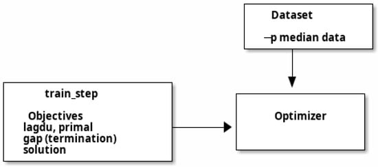
Figure 2. Workflow of Lagrangian Relaxation of p-median problem.

Table 1. p-median datasets used in this study.

Name	Num of Nodes	Num of Edges	Description
Swain55	55	3025	(Swain 1971)
Swain55_big50	2750	7,562,500	randomly interpolated from Swain 55
Swain55_big100	5500	30,250,000	randomly interpolated from Swain 55
Swain55_big200	11,000	121,000,000	randomly interpolated from Swain 55
Swain55_big300	16,500	272,250,000	randomly interpolated from Swain 55

Secondly, we define the functions for computing the primal and dual objectives. As will be discussed in the next sections, the primal function takes a set of values for the location variable as the input and returns a feasible solution for the p-median problem and the associated objective value. The dual function additionally takes a set of multiplier values as input and returns a dual objective value. The dual objective function value is returned by the train_step function in pytorch (version 2.2.1), which is used for gradient descent. Additionally, the difference between the primal and dual objectives is defined as the optimality gap and used as an early termination criterion. Collectively, the primal and dual objective functions form the equivalent of the training step in DL as shown in Figure 2.

Finally, we choose and configure the optimizer, and provide key parameters such as the learning rate, etc. In principle, any stock optimizer in the DL library can be used for the Lagrangian Relaxation solver. By reusing the many standard optimizers, we avoid reinventing the wheel on the various strategies for gradient descent (inertia, dampening factor, etc.) As with traditional DL training process, optimizers can have different speed of convergence. We test different possibilities of optimizer-parameter combinations in the experiment section.

3.2. Lagrangian Relaxation for the p-Median Problem

As discussed in the Background section, the gist of the Lagrangian Relaxation method is to dualize the original optimization problem and transform it into a simpler dual problem that is easier for gradient optimization. In the case of p-median problem in (3) through (6), there is a choice as to which constraints should be relaxed [13]. One possibility is to relax the cardinality constraint (5), so that more than $p$ facilities can be selected (but with an associated cost/penalty). This problem form is exactly a Simple Plant Location Problem (SPLP) and can be solved by the DUALOC algorithm in the literature. We do not take this route because the DUALOC code is very old and not available. The DUALOC algorithm itself is quite complex and difficult to replicate.

Therefore, we use the second option in the literature (see, e.g., [13,14]) and relax the assignment constraint (4). This leads to the following relaxed problem:

$$\mathrm{minimize}\sum _{i\in I}{\mu }_i-\sum _{j\in J}\left(\sum _{i\in I}\left({\mu }_i-a_i\cdot d_{ij}\right)\cdot x_{ij}\right)$$

(11)

Subject To:

$$\sum _{j\in J}{y}_j\le p$$

(12)

$$x_{ij}\le y_j,\forall i\in I,j\in J$$

(13)

$${\mu }_i\ge 0, \forall i\in I$$

(14)

Here, ${\mu }_i$ is the penalty or Lagrangian multiplier associated with each violation of the assignment constraint at customer location $i$ (when $i$ is assigned to more than one facility). The relaxed problem above is still implicit and is not a free function of the decision variables. But one can make it an explicit function of the following form, by taking advantage of the fact that the location variable $y_j$ dominates the allocation variable $x_{ij}$ and at most $p$ of the $y_j$ variables can be non-zero (see [12,13,14]):

$$\mathrm{minimize}\sum _{i\in I}{\mu }_i-\sum _{j\in J}\left(\sum _{i\in I}{\left({\mu }_i-a_i\cdot d_{ij}\right)}^{+}\right)\cdot y_j$$

(15)

s.t.

$$\sum _{j\in J}{y}_j\le p$$

(16)

$${\mu }_i\ge 0, \forall i\in I$$

(17)

where ${\left(x\right)}^{+}:=max\left(x,0\right)$.

Because ${\mu }_i$ is a constant in the Lagrangian dual problem, the dual is indeed a much simpler problem: a sorting problem. One just needs to sort the coefficients of $y_j$, pick the largest $p$ of them, and use their sum in (15) as the dual objective (see [14] for the derivations). Indeed, the dual problem here is much simpler to solve than the original p-median problem (and amenable to gradient computation).

When a solution to the Lagrangian dual problem in (15) through (17) is obtained, there are exactly $p$ facilities in it, and one can easily reconstruct a feasible solution of the primal solution by discarding the $x_{ij}$ values in the dual solution and reconstructing them by assigning each customer $i$ to its closest facility. Therefore, each dual solution gives rise to a primal solution.

3.3. Implementation Issues of p-Median Lagrangian Relaxation Solver

We implement the p-median Lagrangian Relaxation in PyTorch Lightning, a mainstream deep learning framework. The main code for the key components (including the primal function, the Lagrangian dual function and their integration into the PyTorch Lightning library (version 2.5.0)) are presented in Appendix A. Several implementation issues are worth noting:

• GPU friendly data structure and vectorized operation. Compared to ordinary p-median LR-solver, we need to fully utilize the massive parallel computing power of GPGPUs, which can easily have over ten thousand cores. This means that we should avoid writing conventional loops and conditional statements in the code. Instead, we put the distance matrix and decision variables into tensors stored in GPU and use vectorized operations provided by PyTorch everywhere. This includes not only common parallel operations such as matrix multiplication (mm) and sum, but also operations that are not obviously parallel at first glance, such as filter (where), argsort, and min. This brings the power of massive parallel computing for free. As discussed in the next section, GPU-accelerated computation allows us to solve large p-median problems that are unseen in the literature.
• Automatic differentiation computation is made easy. In PyTorch, the (sub-)gradients are calculated and tracked automatically by default. All that was necessary is to place the Lagrangian multipliers ${\mu }_i$ into the parameters() method. This is even easier than directly using the Python pyautograd package as with [14]. In pyautograd, one needs to call explicitly the grad() function on the dual objective function to have its gradient tracked. The grad() takes a Python function as input and returns a new function that computes the gradient of the input function. This is cumbersome and forces the program to be written unintuitively.
• Training step. The training step is implemented in PyTorch Lightning’s training_step() method. We need to compute both the primal objective and the dual objective in this method. Additionally, we apply more precise stopping criteria using the optimality gap (along with standard DL stopping criteria such as the maximum number of iterations and time limit). Note that we only use the dual objective value in gradient descent. This is because the dual objective is what the Lagrangian multipliers act on. The primary objective is only used as an early termination criterion.
• We note that there is no meaningful counterpart for the prediction stage of DL in the GPU-based LR algorithm. In addition, the optimized parameters (the Lagrangian multipliers) are not transferable to other datasets. Therefore, it is not meaningful to save the multiplier results in any model file, unless the intent is to save the intermediate state of the LR algorithm and resume computation later on.

3.4. Contribution and Difference from Traditional Methods

In this article, we have proposed a massively parallel Lagrangian Relaxation-based framework for solving spatial optimization problems using the facilities of Deep Learning and auto-gradient computation. To our best knowledge, no one has proposed such a workflow for Lagrangian Relaxation before. Compared with traditional ways of developing Lagrangian Relaxation, the proposed framework has the following advantages: (1) compared to [14], it makes automatic gradient computation easier to implement by adopting PyTorch functions, making it entirely unnecessary to manually derive and compute (sub)gradients; and (2) it can take advantage of the massive parallelization of GPGPU, allowing large problem instances to be solved in a reasonable amount of time.

Compared with traditional Deep Learning methods. The proposed workflow allows a wider range of optimization problems to be solved by GPGPU. Our objective function in the training_step is more general and can describe any optimization problem. In the original DL workflow, the loss function is defined in a standard way by measuring the difference between NN output calculated using the input data (prediction) and the known output values (ground truth labels). Stock objective functions, such as the RMSprop or entropy, can be chosen from the DL library. In our workflow in Figure 2, we can use a free-form objective function for any optimization problem with well-defined Lagrangian dual. Consequently, we can solve models with more general structures (such as the p-median).

In addition to dual objectives, the LR-based workflow requires a definition of the primal objective function, giving rise to the optimality gap. This provides a true indicator of convergence to the optimal solutions. We use the optimality gap for early termination (i.e., terminate the algorithm when the gap is close enough to zero). By contrast, in traditional DL, we generally do not know whether an optimal solution has been reached when gradient descent stops. This may be fine for many DL applications, but is generally not acceptable for discrete optimization.

4. Experiments

We implemented a GPU-based Lagrangian Relaxation algorithm for the p-median problem using the PyTorch Lightning library according to Figure 2. Most of the code is concentrated in the training_step() method shown in Figure 2, where we compute the Lagrangian dual and primal objectives. The algorithm is terminated when one of the following happens: (i) the optimality gap falls below the threshold value (1%), (ii) the optimality gap does not improve in 2000 iterations, (iii) the pre-specified maximum number of iterations has been reached, or (iv) the pre-specified time limit has been reached. We then executed the CPU and GPU-based experiments on a computer with an Intel i9-13900K CPU, 64 GB of system memory, and an NVIDIA GeForce RTX4090 GPU with 24 GB of video memory. For comparison purposes, we also implemented and solved the p-median problem in IBM ILOG OPL/CPLEX 20.1.

4.1. Data Preparation

We used the classic Swain 55-node dataset [20] as a basis for testing as shown in Figure 3. Each dot represents a customer location and a candidate site for facilities. The nodes are labeled in descending order of the population. So the central region has a higher population concentration. We first tested the GPGPU-based LR algorithm on the original Swain dataset. While we obtained the same solutions as known results in the literature, the original Swain dataset (and existing p-median datasets) is too small for GPGPU and parallel processing to be profitable. The overhead associated with communicating with GPGPU may overwhelm the speedup from the parallelization. To properly test the power of the GPU-enabled LR algorithm, we generated much larger datasets by densifying the Swain dataset, as follows. We add new customer points randomly around each original customer point such that the new customer locations follow a uniform distribution with a width of 3.0 (about one twentieth of the map width). We then randomly disturbed the population of each customer location by 3 (where the original population range is between 2 and 71). This is intended to mimic the spatial distribution of the population in the Swain dataset. The densified test dataset is much bigger (50, 100, 200, 300 times bigger). And these data are much bigger than any p-median dataset solved by optimal algorithms. The sizes of the test datasets are presented in Table 1. The Swain datasets have dense distance matrices. Therefore, for an $n$ node dataset, the number of edges (possible assignments) is $n^2$.

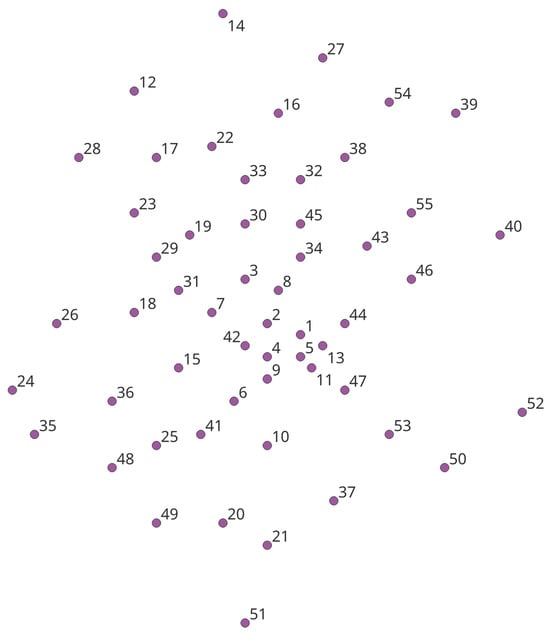
Figure 3. The base Swain 55 node datasets (Swain, 1971). Each dot is simultaneously a customer location and a candidate site.

4.2. Correctness

We use the original Swain 55-node dataset to test the correctness of our LR algorithm. Figure 4 presents the progress of the dual and primal objectives with the increase in iterations for the GPU-based LR algorithm. The optimizer is Adamax, the learning rate is 0.015625, and the number of facilities ($p$) is 5. We can observe that the dual and primal objective curves converge gradually (after about 16,000 iterations) to a value of about 2950. By the principle of strong duality, this means that 2950 is the optimal objective value, which concurs with results in the literature.

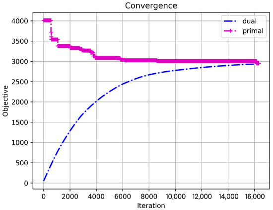
Figure 4. Convergence: the number of iteration vs. the primal and dual objectives for the GPU-based LR algorithm (Adamax optimizer, p = 5).

4.3. Solution Characteristics

Figure 5 presents the trend of the objective function values for the GPU/CPU versions of the LR algorithms and the OPL solver for values of $p$ in 5, 400, 800, 1200, 1600, and 2000, respectively. The $p$ values are chosen to range from a value near zero to roughly half of the number of customer locations ($\left|I\right|$). We can observe a decreasing trend of the objective value as $p$ increases. This is correct because, with more servers, the total service distance to population centers always decreases. The objective function values for the three algorithms agree at all $p$ values, except for $p=5$, where the OPL solver produced a larger objective value. This is because the OPL solver did not converge in the one-hour time limit in this particular case.

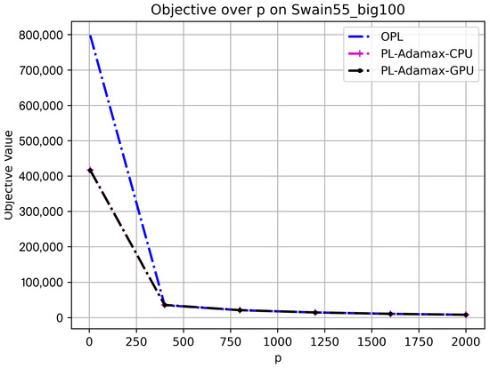
Figure 5. Solution characteristics: objective function value vs. p on Swain55_big100 dataset, lr_rate = 0.015625.

4.4. Computational Time and Comparison with CPU-Based Algorithms

Figure 6 presents the computational times for the GPU- and CPU-based Lagrangian algorithms, and a comparison with the MILP solver (OPL). We tested the Swain55_big100 dataset (with 5500 nodes) using a learning rate of 0.015625 and $p$ values of 5, 400, 800, 1200, 1600, and 2000. A one-hour time limit was imposed. From Figure 6, we can observe that the computational times of the GPU-based Lagrangian Relaxation algorithm are significantly superior to those of the conventional CPU-based OPL solver. Moreover, even the CPU version of the LR algorithm is consistently faster than OPL. At p = 400, the speedup of the GPU-based LR algorithm over OPL is 113.9, while the speedup over CPU LR algorithm is 11.3; at p = 2000, the speedup over OPL is 102.7 and the speedup over the CPU version is 15.9. On average, the solution time for the GPU LR algorithm is one minute, the speedup over OPL is 104.9, and the speedup over the CPU version of LR is 12.5. The observed GPU utilization is approximately 90% on average.

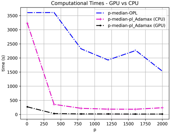
Figure 6. Computational times for the GPU-based LR, CPU-based LR and OPL-based algorithms, where p = 5, 400, 800, 1200, 1600, 2000, and the learning rate = 0.015625.

The computational times in the previous figure reflect both the speed of the LR algorithm and the effectiveness of the processors in CPU and GPU. To investigate the speed of the algorithm alone, we plot in Figure 7 for each $p$ the number of iterations it took the algorithm to terminate using the same dataset, $p$, and learning rate as used in Figure 6. Now that we count the speed in terms of the number of iterations, we can observe that the speeds of the GPU- and CPU-based LR algorithms are really the same. In addition, Figure 7 shows that the numbers of iterations to termination are generally low (below 10,000) when the $p$ value is greater than or equal to 400. This pattern is different from conventional heuristic algorithms, such as the interchange heuristics of [11], or algorithms such as simulated annealing, and genetic algorithms. In those heuristic algorithms, the size of the search space for solution depends on $p$ and a greater $p$ means a (much) greater number of facility combinations to consider. In contrast, in our LR algorithm, the size of the gradient vector (${\mu }_i$) is constant and does not vary with increase in the $p$ value.

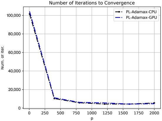
Figure 7. The total number of iterations at each value of p.

4.5. Sensitivity of Learning Rate

As discussed in the previous section, the learning rate $\tau$ is a key parameter influencing the speed or convergence of the gradient descent process. To understand its influence, we plot in Figure 8 the final optimality gap for the GPU-based LR algorithm for a series of $\tau$ values, after 40,000 iterations or 10 days are reached. The algorithm also terminates when there is no improvement in 2000 iterations, as described in the previous section. The test data is Swain55_big100, p = 5, and $\tau$ is chosen to grow exponentially from $2^{-10}$ to $2^{10}$ (with each $\tau$ value twice the previous one). We can observe that the curve has a “U” shape, and the LR algorithm converges when $\tau$ is in the range of $2^{-4}$ to 1. The farther $\tau$ is away from this central region, the greater the optimality gap. This means that the learning rate should not be too large or too small. Otherwise, the LR algorithm may either oscillate or progress too slowly.

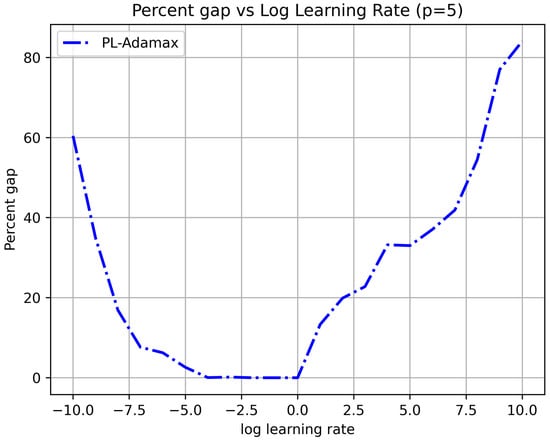
Figure 8. Learning rate vs. gap percentage, Swain55_big100, p = 5.

Similar to Figure 8, Figure 9 presents a sensitivity analysis of the learning rate versus the number of iterations. We can observe a general decreasing trend in the number of iterations with an increase in the learning rate $\tau$. In particular, the LR algorithm maximizes the 40,000-iteration limit when $\tau$ is less than or equal to $2^{-5}$. So, in Figure 8, on the left side of the curve, the algorithm does not converge because the gradient descent is too slow and exceeds the time limit, whereas on the right side of the curve, the algorithm does not converge, presumably because of oscillation.

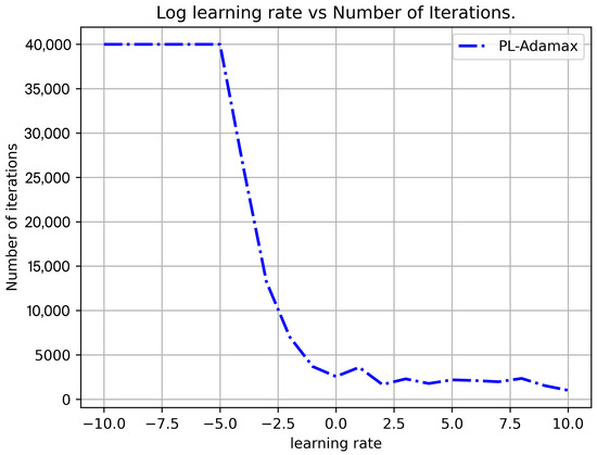
Figure 9. Learning rate vs. Number of Iterations, Swain55_big100, p = 5.

4.6. Comparing Different Optimizers

One advantage of the proposed LR algorithm is that it can utilize the many stock optimizers without reinventing the wheel. Figure 10 presents the convergence behavior of several different optimizers under the same settings as those in Figure 8, except for the optimizer. The optimizers include the prototypical SGD, the Rprop, and variants of the Adam optimizers (Adamax, NAdam, and RAdam). From the figure, the curves for all optimizers have a U-shape similar to Figure 8, except for Rprop, which does not converge at any $\tau$ value. The Adam family of optimizers seems to outperform the others, with RAdam and Adamax achieving convergence in approximately the same range of learning rates ($2^{-5}$ to $2^0$). This is the reason we chose the Adamax optimizer as the default for all previous experiments. This figure demonstrates that although their performance varies, optimizers can be used interchangeably in our GPU-based framework.

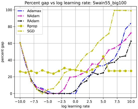
Figure 10. Comparing convergence between optimizers.

4.7. Comparing Different Datasets

Similar to Figure 10, Figure 11 present the convergence behavior of the GPU-based algorithm over different datasets: Swain55, Swain55_big50, Swain55_big200, and Swain55_big300, respectively. In each sub-figure, we can observe the same U-shaped curves of optimality gap vs. learning rate. The convergent ranges of learning rates seem to be wider for smaller datasets than bigger datasets. For example, for the Swain55 dataset, all optimizers have a common range that is quite wide (from $2^{-7}$ to $2^1$). For the biggest Swain55_big300 dataset, only the Adamax and RAdam optimizers have a convergent range between $2^{-5}$ to $2^{-3}$. This intuitively indicates that bigger problems are harder to solve.

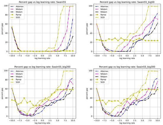
Figure 11. Comparing convergence among optimizers and different datasets.

5. Conclusions

Spatial optimization is an integral part of GIS, and effective algorithms for spatial optimization problems are crucial for its success. In this article, we presented a GPU-based effective Lagrangian Relaxation algorithm for the classic p-median problem, which integrates massive parallel computing, the tool-chain of deep learning, and gradient optimization. Fundamentally, this is based on a comparison of general optimization and deep learning, which allowed us to combine the powers of both worlds and write LR algorithms using the language of deep learning. In particular, we showed how general optimization corresponds to the training step of deep learning, and that standard optimizers in DL libraries can be reused without modification for general optimization. One only needs to adapt the training step and incorporate more general objective functions. In the case of LR, both the Lagrangian dual and the primal objectives need to be computed in the training_step, and the gradient vector needs to be specified as a parameter of the optimizer.

The main findings of this research are that

• Implementing the p-median LR solver in a deep learning library is not only feasible but also convenient. It saves work in implementing a sophisticated optimization strategy and avoids reinventing the wheel. One can focus on defining the Lagrangian dual problem and then use the many standard optimizers interchangeably.
• Automatic gradient (autograd) computation is made easy during implementation and comes with the capability of built-in parallel computing.
• Not all optimizers perform equally. The Adam family of optimizers (especially Adamax) seems to outperform the others in solving large p-median problems (with over 10,000 nodes).
• The learning rate is a key factor in deciding the performance of the LR optimization. Generally, there is a contiguous region of learning rate values in which the LR algorithm converges.

There are several advantages of this research. Firstly, unlike traditional heuristic and deep learning algorithms, the Lagrangian Relaxation-based algorithm provides the optimality gap and certificate of optimality. This serves as a true stopping criterion for gradient descent. Secondly, unlike conventional methods such as mathematical programming, the LR algorithm is efficient and much faster. As demonstrated by the experiments, the LR effectively takes advantage of the massive parallelization of GPGPU and can be 100 times faster than the fastest mathematical programming solvers such as OPL/CPLEX in solving the p-median problem. Thirdly, reusing the stock optimizers from DL allows one to avoid reinventing the wheel (for gradient descent). The auto-gradient capabilities of modern DL libraries also reduce much of the work in tracking gradients.

Due to the generality of the p-median problem, we expect that the proposed GPU-based LR method can be applied to other types of spatial optimization problems to reduce computation time and ease algorithmic development. This includes the classic location problems such as the SPLP, the maximal covering location problem and the hub median location problems. As said earlier, the p-median problem (and its extensions) has been used as unified solvers for other types of spatial optimization models. This idea could be implemented in GPU-enabled GIS systems to find optimal or near-optimal solutions for various spatial optimization problems.

Although we have demonstrated the feasibility of integrating modern DL and Lagrangian Relaxation, there are several areas worthy of future research. Firstly, one could investigate deeper integration of the DL facilities and Lagrangian Relaxation. In this article, we used the basic grid search method to find good learning rates. This is time-consuming and inflexible. One could adapt existing DL tools for parameter tuning for use in writing LR algorithms. Secondly, the size of datasets is limited by the size of the GPU memory. The largest dataset we could test is Swain55_big300 with 16,500 nodes due to this constraint. It would be worthwhile to search for a more effective representation of the p-median problem (e.g., using sparse rather than dense distance matrices) to reduce GPU memory consumption. Alternatively, an interesting question is whether mini-batches can be adapted in DL for use in GPU-based LR algorithms. Finally, one could implement existing gradient descent loops in LR algorithms as optimizers that can be reused in a standard way. It would be interesting to investigate how they compare with the stock optimizers in DL libraries. This is left as future work.

References

- Hakimi, S.L. Optimum Locations of Switching Centers and the Absolute Centers and Medians of a Graph. Oper. Res. 1964, 12, 450–459. [Google Scholar] [CrossRef]
- Hakimi, S.L. Optimum Distribution of Switching Centers in a Communication Network and Some Related Graph Theoretic Problems. Oper. Res. 1965, 13, 462–475. [Google Scholar] [CrossRef]
- Goldman, A.J. Optimal Locations for Centers in a Network. Transp. Sci. 1969, 3, 352–360. [Google Scholar] [CrossRef]
- Hakimi, S.L.; Maheshwari, S.N. Optimum Locations of Centers in Networks. Oper. Res. 1972, 20, 967–973. [Google Scholar] [CrossRef]
- Hillsman, E.L. The p-Median Structure as a Unified Linear Model for Location-Allocation Analysis. Environ. Plan. A 1984, 16, 305–318. [Google Scholar] [CrossRef]
- Manne, A.S. Plant Location Under Economies-of-Scale-Decentralization and Computation. Manag. Sci. 1964, 11, 213–235. [Google Scholar] [CrossRef]
- Church, R.L.; ReVelle, C. The Maximal Covering Location Problem. Pap. Reg. Sci. Assoc. 1974, 32, 101–118. [Google Scholar] [CrossRef]
- O’Kelly, M.E. The Location of Interacting Hub Facilities. Transp. Sci. 1986, 20, 92–106. [Google Scholar] [CrossRef]
- Lei, T.L.; Church, R.L.; Lei, Z. A Unified Approach for Location-Allocation Analysis: Integrating GIS, Distributed Computing and Spatial Optimization. Int. J. Geogr. Inf. Sci. 2016, 30, 515–534. [Google Scholar] [CrossRef]
- Imai, A.; Nishimura, E.; Current, J. A Lagrangian Relaxation-Based Heuristic for the Vehicle Routing with Full Container Load. Eur. J. Oper. Res. 2007, 176, 87–105. [Google Scholar] [CrossRef]
- Teitz, M.B.; Bart, P. Heuristic Methods for Estimating the Generalized Vertex Median of a Weighted Graph. Oper. Res. 1968, 16, 955–961. [Google Scholar] [CrossRef]
- Fisher, M.L. The Lagrangian Relaxation Method for Solving Integer Programming Problems. Manag. Sci. 1981, 27, 1–18. [Google Scholar] [CrossRef]
- Hanjoul, P.; Peeters, D. A Comparison of Two Dual-Based Procedures for Solving the p-Median Problem. Eur. J. Oper. Res. 1985, 20, 387–396. [Google Scholar] [CrossRef]
- Lei, Z.; Lei, T.L. Solving Spatial Optimization Problems via Lagrangian Relaxation and Automatic Gradient Computation. ISPRS Int. J. Geo-Inf. 2025, 14, 15. [Google Scholar] [CrossRef]
- Krizhevsky, A.; Sutskever, I.; Hinton, G.E. ImageNet Classification with Deep Convolutional Neural Networks. Commun. ACM 2017, 60, 84–90. [Google Scholar] [CrossRef]
- Vaswani, A.; Shazeer, N.; Parmar, N.; Uszkoreit, J.; Jones, L.; Gomez, A.N.; Kaiser, Ł.; Polosukhin, I. Attention Is All You Need. In Proceedings of the 31st Annual Conference on Neural Information Processing Systems (NIPS), LA Jolla, CA, USA, 4–9 December 2017. [Google Scholar]
- ReVelle, C.S.; Swain, R.W. Central Facilities Location. Geogr. Anal. 1970, 2, 30–42. [Google Scholar] [CrossRef]
- Held, M.; Wolfe, P.; Crowder, H.P. Validation of Subgradient Optimization. Math. Program. 1974, 6, 62–88. [Google Scholar] [CrossRef]
- Kingma, D.P.; Ba, J. Adam: A Method for Stochastic Optimization. In Proceedings of the International Conference on Learning Representations (ICLR), San Diego, CA, USA, 7–9 May 2015. [Google Scholar]
- Swain, R.W. A Decomposition Algorithm for a Class of Facility Location Problems. Ph.D. Thesis, Cornell University, Ithaca, NY, USA, 1971. [Google Scholar]
Disclaimer/Publisher’s Note: The statements, opinions and data contained in all publications are solely those of the individual author(s) and contributor(s) and not of MDPI and/or the editor(s). MDPI and/or the editor(s) disclaim responsibility for any injury to people or property resulting from any ideas, methods, instructions or products referred to in the content. |
© 2025 by the authors. Published by MDPI on behalf of the International Society for Photogrammetry and Remote Sensing. Licensee MDPI, Basel, Switzerland. This article is an open access article distributed under the terms and conditions of the Creative Commons Attribution (CC BY) license (https://creativecommons.org/licenses/by/4.0/).