Article

LA-GATs: A Multi-Feature Constrained and Spatially Adaptive Graph Attention Network for Building Clustering

1
Aerial Photogrammetry and Remote Sensing Group Co., Ltd., Xi’an 710000, China
2
School of Systems Science and Engineering, Sun Yat-sen University, Guangzhou 510006, China
*
Author to whom correspondence should be addressed.
ISPRS Int. J. Geo-Inf. 2025, 14(11), 415; https://doi.org/10.3390/ijgi14110415
Submission received: 10 August 2025 / Revised: 18 October 2025 / Accepted: 20 October 2025 / Published: 23 October 2025

Abstract

Building clustering is a key challenge in cartographic generalization, where the goal is to group spatially related buildings into semantically coherent clusters while preserving the true distribution patterns of urban structures. Existing methods often rely on either spatial distance or building feature similarity alone, leading to clusters that sacrifice either accuracy or spatial continuity. Moreover, most deep learning-based approaches, including graph attention networks (GATs), fail to explicitly incorporate spatial distance constraints and typically restrict message passing to first-order neighborhoods, limiting their ability to capture long-range structural dependencies. To address these issues, this paper proposes LA-GATs, a multi-feature constrained and spatially adaptive building clustering network. First, a Delaunay triangulation is constructed based on nearest-neighbor distances to represent spatial topology, and a heterogeneous feature matrix is built by integrating architectural spatial features, including compactness, orientation, color, and height. Then, a spatial distance-constrained attention mechanism is designed, where attention weights are adjusted using a distance decay function to enhance local spatial correlation. A second-order neighborhood aggregation strategy is further introduced to extend message propagation and mitigate the impact of triangulation errors. Finally, spectral clustering is performed on the learned similarity matrix. Comprehensive experimental validation on real-world datasets from Xi’an and Beijing, showing that LA-GATs outperforms existing clustering methods in both compactness, silhouette coefficient and adjusted rand index, with up to about 21% improvement in residential clustering accuracy.

1. Introduction

The spatial distribution patterns of urban buildings are fundamental to understanding urban morphology and achieving intelligent urban planning. As cities continue to expand in scale and spatial complexity, accurately identifying and classifying the relationships between buildings has become increasingly important [1,2]. Building clustering, as an effective analytical tool, plays a crucial role in modern urban planning and the development of smart cities. By grouping buildings that are spatially adjacent, geometrically similar, or functionally related, building clustering not only helps reveal the internal structural patterns of cities but also provides essential decision support for urban planning, traffic optimization, and resource allocation [3,4,5].
The goal of building clustering is to group buildings with spatial proximity, similar forms, or related functions into semantically consistent clusters. However, due to the complexity of urban building clusters in terms of spatial distribution, geometric features, and appearance properties, building clustering differs from traditional point clustering methods [6]. Traditional methods typically rely on Euclidean distance or similarity measures based on a single feature (e.g., building area). These methods often consider only the impact of a single feature on the similarity between buildings, resulting in clustering outcomes constrained by that single feature. For the fusion of a small number of features (e.g., simultaneously considering building orientation and area), these methods lack flexibility in calculating feature weights, making it difficult to fully reflect the importance and interrelationships of the features [7]. Additionally, building clustering often incorporates the quantification of Gestalt principles as constraints [8,9]. While Gestalt principles aid in understanding how we visually perceive relationships between buildings, their quantification standards have not been widely standardized. As a result, buildings are influenced by factors such as proximity, similarity, and continuity, which are difficult to quantify using traditional Euclidean distance metrics [10,11]. For example, when two buildings are symmetrically arranged (aligning with the symmetry principle in Gestalt theory), their spatial layouts may be similar, but their direction, color, and other features may exhibit “discontinuous” changes, meaning these features do not change smoothly. This “discontinuous” variation can affect the accuracy of building clustering. Therefore, relying solely on a single feature or a few features often fails to produce clustering results that accurately reflect the actual distribution. Consequently, traditional clustering methods often struggle to balance multi-dimensional similarity measures with the preservation of local spatial structures [7], leading to clustering results that lack continuity and semantic coherence, and fail to closely match the actual distribution patterns of buildings [12].
To overcome the limitations of traditional methods, machine learning-based approaches have increasingly emerged as effective solutions for clustering [13]. In recent years, attention mechanisms, with their powerful feature fusion capabilities and ability to model long-range dependencies, have shown significant advantages in the analysis of visual and spatial data. Within the framework of Graph Neural Networks (GNNs), Graph Attention Networks (GATs), as an important variant, extend GNNs by incorporating explicit attention mechanisms [14,15]. Moreover, the effectiveness of GNN-based clustering methods has been well validated [16,17,18,19]. GATs possess strong transfer learning capabilities, enabling them to adaptively learn the importance of different neighbors based on graph structure, node features, and varying weight distributions. By assigning different weights to each neighbor, GATs can flexibly capture the relationships between buildings. Compared to traditional CNN-based methods and graph partitioning techniques, GATs are better suited for capturing the complex relationships between buildings. However, how to fully leverage the advantages of GATs in feature fusion, neighborhood modeling, and attention mechanism design for more effective building clustering remains a topic that warrants further investigation. This paper proposes a building clustering method based on GATs, aiming to integrate multiple features of buildings and fully leverage the multi-head attention mechanism to model the adjacency relationships between buildings, adaptively assigning feature weights, thereby further improving the accuracy of building clustering.
The remainder of this paper is organized as follows: Section 2 briefly reviews relevant research on building clustering; Section 3 introduces a building clustering method based on an improved graph attention network; Section 4 presents experimental analyses and results; and Section 5 summarizes the research findings and discusses future improvement strategies.

2. Related Work

Building clustering, as a key component of cartographic generalization and urban modeling, aims to organize buildings into semantically coherent groups based on their morphology, function, spatial location, and structural characteristics, thereby facilitating automated representation and analysis of building groups. The existing research can be broadly classified into clustering based on spatial distance, semantic similarity, and graph theory, based on different similarity measurement standards.
Spatial distance-based methods typically group buildings based on their spatial proximity and have been the earliest and most widely used clustering techniques [20]. Among these, the Density-Based Spatial Clustering of Applications with Noise (DBSCAN) algorithm has been widely applied in building clustering. However, such methods often rely on global thresholds, and their clustering performance significantly deteriorates when the building density distribution varies greatly. Rodrigues and Léo [21] proposed a density peak-based clustering method that introduced an optimization mechanism to adapt to local density variations, improving its performance in datasets with uneven density. However, these methods remain sensitive to irregular spatial distributions, noise, and outliers, and they struggle to simultaneously utilize semantic or geometric features of buildings during clustering. Moreover, building clustering differs notably from traditional clustering, as the distance between buildings is not limited to Euclidean space. When measuring the distance between buildings, factors such as building height, size, color, and orientation must also be considered. Ai and Guo [9] introduced the concept of visual distance, incorporating features like orientation and compactness into traditional Euclidean distance calculations. While innovative, this approach relied solely on a single feature for weighting, making it inefficient in multi-dimensional contexts. Qi and Li [11] considered the proximity, alignment, and similarity constraints from Gestalt principles for MST clustering, and evaluated the priority of these three principles. Additionally, Deng et al. [7] reviewed existing building clustering methods based on Gestalt principles and discussed the impact of applying single Gestalt principles or combinations of multiple principles in real-world applications.
Semantic similarity-based clustering: Liu et al. [22] proposed a method for identifying spatial distribution patterns of buildings from the perspective of dual spatial semantic constraints. This method outperforms mainstream methods at the time in constructing clustering tasks. Jin et al. [23] measured the similarity between buildings using attributes such as shape narrowness, area ratio, concavity, distance, and connectivity, and their experimental results improved clustering performance to some extent. Yan [24] considered six factors from Gestalt principles to describe residential structures, morphology, and relationships, and clustered buildings based on proximity and similarity using an iterative approach. They argued that proximity is the optimal criterion for evaluating building spatial distribution patterns, although their experiments involved a significant number of parameters, affecting scalability. Gao et al. [25] measured the similarity of features in terms of function and attributes, demonstrating that their clustering results are highly consistent with human visual perception. However, accurately capturing semantic information remains a challenge.
The graph-based clustering method provides a different approach compared to the first two clustering methods. It not only focuses on the physical spatial relationships and semantic relationships between buildings but also uses the structure of a graph to describe and analyze the complex relationships between buildings. In graph-based methods, buildings are treated as nodes in the graph, and the edges between the nodes represent the relationships between the buildings (such as adjacency, similarity, or functional associations). Graph-based clustering analyzes the graph’s topological structure (such as minimum spanning trees, graph convolutions, etc.) to uncover hidden relationships between buildings, effectively handling non-Euclidean relationships and higher-order dependencies. Regnauld [26,27] considered Gestalt parameters like average size, shape, and density of building groups, constructing a Delaunay triangulation and using the minimum spanning tree (MST) to obtain the final clustering result. Sun et al. [28] further expanded on visual distance by introducing multiple features and using MST for clustering, but the weight distribution of multiple features relied on manual adjustment. Spectral clustering combines topological features of graphs with multi-dimensional attribute information of nodes, utilizing dimensionality reduction techniques to handle high-dimensional data for effective clustering analysis [29]. Dimensionality reduction significantly improves model clustering performance on non-linear datasets [30,31]. Tang et al. [32] proposed a spectral clustering-based community detection method that converts node distances into similarity using a Gaussian kernel function, thereby constructing a similarity matrix. However, they noted that the method has limitations in sparse clustering. Furthermore, clustering algorithms combining deep learning have become a popular research topic in recent years. Zhang et al. [33] integrated graph structure and feature information into the kernel matrix using high-order graph convolution. Kang et al. [34] constructed a graph describing the relationship between samples, anchor points, and single-view and multi-view data to improve clustering performance. Berahmand et al. [35] proposed a new community detection attribution spectral clustering method that integrates network topology and node attributes to improve clustering accuracy. Yan et al. [36] proposed a graph convolutional network method to train the distance between nodes and center nodes, and then used K-means clustering to group buildings. However, this method relies on manually labeled true clustering numbers. Chen et al. [6] addressed the issue of adaptive learning of multi-feature weights using Graph Attention Networks (GAT), but their similarity computation neglected the crucial spatial distance factor, and message passing was restricted to first-order neighborhoods, making it susceptible to graph construction errors.
In summary, graph theory-based clustering algorithms have become a hot research topic due to their strong nonlinear partitioning capabilities. Furthermore, the integration of graph theory methods with graph deep learning has further enhanced model performance. The multi-feature constrained and spatially adaptive building clustering network (LA-GATs) proposed in this paper is a clustering method combining graph theory and graph deep learning. By introducing the graph attention mechanism, LA-GATs can more accurately capture the similarity between buildings, thereby improving clustering accuracy and reducing manual intervention. The main advantages of this method are: ① Traditional spatial distance methods often rely on a single or a few features (such as Euclidean distance), which fail to accurately reflect the multidimensional relationships between buildings. In this paper, we enhance the accuracy of similarity calculation by integrating multi-source heterogeneous building features; ② Some existing methods (such as DBSCAN) depend on global thresholds, and their clustering performance deteriorates significantly when the building density distribution varies greatly. To address this, we introduce a distance bias term during training to ensure that the clustering results better align with the first law of geography; ③ Existing graph-based clustering methods (such as graph convolution-based algorithms) are often limited by graph construction errors, which affect the authenticity of clustering results. In this paper, we introduce a second-order neighborhood aggregation strategy to effectively reduce the propagation of graph construction errors, thereby enhancing the authenticity of clustering results.

3. Materials and Methods

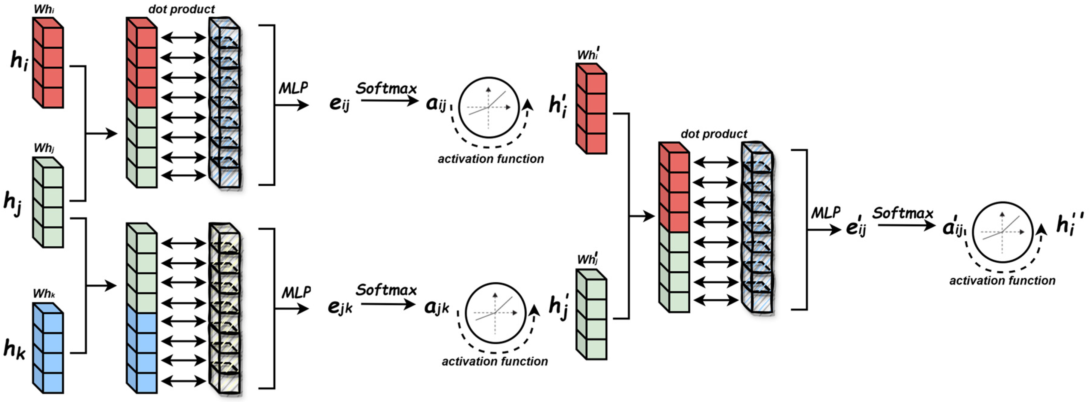
The self-attention mechanism introduced in this study for building clustering is primarily implemented through multi-similarity feature fusion and local spatial relationship modeling. The core idea is to transform complex inter-building associations—such as distance, orientation, morphology, and color—into learnable attention weights, thereby adaptively capturing the intrinsic grouping patterns within building clusters, as illustrated in Figure 1.
The building clustering based on LA-GATs can be divided into three steps:
  • Step 1: Building the dataset. The geometric, appearance, and spatial attributes of each building are encoded into feature vectors to construct the initial feature matrix. Considering the computational complexity of the features, this study selects four features—compactness, orientation, color, and height—for training. Previous research has demonstrated that these features align with Gestalt principles and, when applied to building clustering, provide visual perceptual constraints that help to more accurately identify the distribution patterns of buildings [9,23,24,28]. Subsequently, heterogeneous feature matrices are computed (e.g., Euclidean distance, directional angle differences, and color histogram differences) to quantify the multi-dimensional relationships between buildings.
  • Step 2: Building the feature similarity matrix. Pass the feature matrix as input to the Graph Attention Network (GAT). During the learning of attention coefficients, a distance bias term (distance decay factor) is incorporated to ensure continuity in the spatial distribution of buildings. A multi-head attention mechanism is adopted to improve model accuracy and enhance the stability of feature representation, while a second-order neighborhood aggregation strategy is employed to mitigate the propagation of errors caused by imperfections in Delaunay triangulation construction.
  • Step 3: Spectral Clustering. The input for spectral clustering is obtained by calculating the similarity matrix. The optimal number of clusters is determined using the elbow method [37], and then clustering is performed by eigen-decomposition of the normalized Laplacian matrix.

3.1. Feature Design for Buildings

The spatial distribution pattern is an interrelated structure formed by the arrangement and distribution of spatial objects [12]. In recognizing these distribution patterns, human cognition is often guided by certain fundamental principles. Gestalt theory provides an effective visual perception framework that constrains spatial relationships from an overall scene perspective, making the spatial relationships between adjacent objects more in line with human cognitive patterns [9,11]. In the building clustering process, some geometric characteristics of buildings happen to align with Gestalt principles, allowing us to apply various Gestalt principles to analyze building clustering and better reflect their spatial relationships. Common Gestalt principles include proximity, similarity, orientation, closure, continuity, connectedness, common fate, and common region [38].
The main purpose of this paper is to verify the feasibility of multi-feature fusion in LA-GATs for building clustering. Therefore, this experiment only considers commonly used Gestalt principles in previous studies, such as the proximity, orientation, and similarity principles [28]. Specifically, the proximity principle suggests that two objects that are close to each other can be grouped together. In this paper, the proximity principle is represented by the proximity distance between buildings, which forms the basis for constructing the nearest neighbor graph. Based on this nearest neighbor graph, we calculate the similarity matrix between buildings. The orientation principle suggests that objects with similar alignment can be grouped together. In this study, we directly use the orientation of buildings to describe this feature, with specific methods detailed in Section 3.2. The similarity principle suggests that objects with similar shapes or sizes can be grouped together based on visual perception. In this study, this feature is represented by compactness, height, and color. Compactness is closely related to the spatial occupation and morphological features of buildings; height and color are significant visual identifiers in human perception. According to Gestalt principles, these features effectively reflect the similarity and group affiliation between buildings, helping to capture the spatial distribution patterns of buildings more accurately.
Additionally, compactness, height, and color are easily accessible features with low computational complexity, making them suitable for direct modeling and calculation. Compared to other potentially more complex or costly features (such as concavity, roof texture, etc.), these three features offer significant advantages in computational efficiency, while also aligning well with the goals of this experiment, allowing for effective validation of the multi-feature fusion method.

3.2. Building Feature Extraction

Building feature extraction is the first critical step of the proposed method. It involves identifying and analyzing characteristics such as the shape, structure, and texture of buildings [39]. In this stage, we primarily construct the dataset required for the feature matrix in the Graph Attention Network (GAT).

3.2.1. Orientation Feature

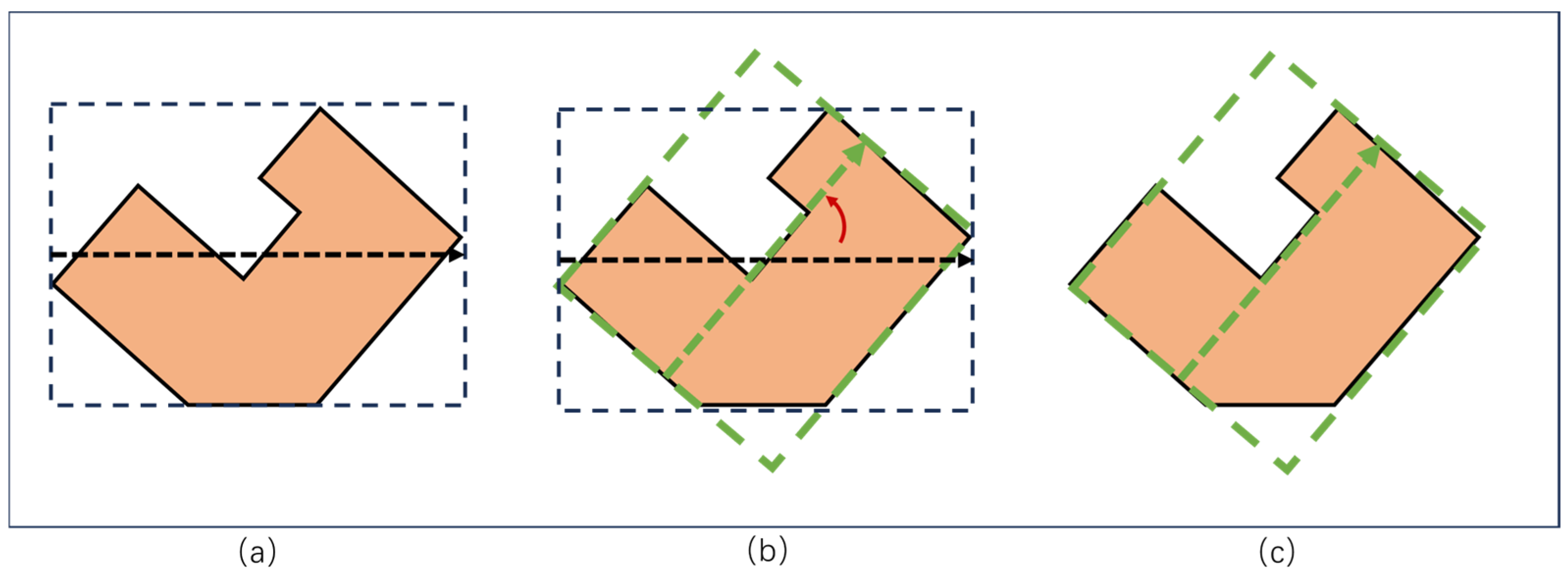
The Minimum Bounding Rectangle (MBR) method refers to the smallest-area (or smallest-volume) rectangle that completely contains a given two-dimensional or three-dimensional geometric object, such as a set of points, polygons, or line segments. Among all possible bounding rectangles, the MBR is the one with the minimal area. In this study, the MBR is employed as the orientation feature of buildings [40]. By rotating the building geometry and computing the rotation angle corresponding to its MBR, we can effectively capture the true directional orientation of the building. The calculation method for the MBR direction is shown in Figure 2.

3.2.2. Compactness Feature

The compactness feature is primarily used to represent the shape characteristics of buildings [41]. Due to the complexity and irregularity of building polygons, earlier studies on linear features often quantified shape factors using a single parameter. Compactness provides an effective measure for capturing the geometric complexity of buildings: higher compactness values generally indicate more complex shapes. It is commonly computed as the ratio of the building’s area to its perimeter, expressed as:
C = p e r i m e t e r ( b ) 2 π A r e a ( b )
where p e r i m e t e r ( b ) denotes the perimeter of building b , A r e a ( b ) denotes the area of building b , and C represents the compactness of the individual building.

3.2.3. Other Features

In addition to the aforementioned features, the dataset used in this study also incorporates building color and height attributes [42,43]. The color feature is represented as a single-value descriptor computed using the perceptual hash (pHash) method, while the height feature is obtained by averaging sampled points from the building’s rooftop [44,45]. As these features are not the primary focus of this work, they are not analyzed in detail here.

3.3. Spatial Relationship Modeling

In this step, we investigate how to compute the proximity distances between buildings and use these distances to construct a nearest-neighbor graph, which serves as the adjacency matrix input for the Graph Attention Networks (GATs) in our method.

3.3.1. Constrained Delaunay Triangulation

The Delaunay Triangulation possesses two key properties—the circumcircle property and the nearest-neighbor connection property—which enable it to accurately model the proximity relationships among spatial objects. It has been widely applied in tasks such as spatial conflict detection and spatial distance computation [46]. In a general triangulation, elongated triangles often occur, where one angle is very small or one edge is excessively long. In contrast, the circumcircle property of the Delaunay Triangulation minimizes the occurrence of such elongated triangles and maintains relatively balanced interior angles. Using a Delaunay Triangulation helps preserve the local spatial continuity of buildings.
When constructing a triangulation among buildings, the generated triangles must not cross building boundaries. Therefore, during the triangulation process, building edges are enforced as triangle edges, forming what is known as a Constrained Delaunay Triangulation (CDT) [47,48]. In practice, due to the complex and diverse structures of buildings, constructing a triangulation solely from polygon vertices may fail to satisfy the nearest-neighbor connection property. To address this, additional points are generated along building boundaries to ensure compliance with Delaunay construction rules—a process referred to as boundary point interpolation (Figure 3).
The encryption process is roughly as follows:
  • Step 1: Perform point interpolation encryption on the polygon boundary vector points;
  • Step 2: Construct the Delaunay triangulation;
  • Step 3: Embed the constraint edges to form a constrained Delaunay triangulation, achieving triangulation refinement.

3.3.2. Computing the Nearest Distance

The proximity between two buildings is determined from the CDT edges that connect points on their boundaries. The length of the shortest such edge is initially taken as the spatial distance.
For simple building geometries, this distance can be approximated using the minimum vertex-to-vertex distance or the minimum distance between vertices of their Minimum Bounding Rectangles (MBRs). However, for more complex building geometries, the adjacency distance provides a more meaningful measure, as it incorporates line-of-sight (LoS) information—representing the unobstructed space between buildings.
The original adjacency distance is computed as:
A d j d i s P , Q = 1 n i = 1 n h e i g h t i
where h e i g h t i denotes the height of each LoS triangle between buildings P and Q , and n is the number of such triangles in the LoS region.
In this study, we extend the definition to improve computational efficiency while retaining the semantic meaning of visual connectivity:
A d j d i s = A r e a 1 n i = 1 n h i
where h i denotes the height at each LoS sampling point and A r e a denotes the shared visual field area of the LoS region. This formulation reduces computational load while preserving key geometric relationships.
To ensure accurate representation of spatial connectivity, CDT triangles are classified into three types (Figure 4): Type 1: Vertices belong to two or three different building polygons. Type 2: Vertices lie on the same building polygon but the triangle is located outside any building. Type 3: Vertices lie on the same building polygon and the triangle lies entirely within that building. Type 1 and Type 2 triangles are defined as true connection triangles, while Type 3 triangles are false connection triangles. False connections are removed, ensuring that only true connections represent valid adjacency between buildings.

3.3.3. Construction of the Nearest-Neighbor Graph

The nearest neighbor graph serves as the basis for constructing the building feature matrix. It is constructed using the Constrained Delaunay Triangulation (CDT). In the triangulation generated from the CDT, if there exists at least one Type 1 connection triangle between two building polygons, the two buildings are considered to have spatial adjacency [49].
Based on these adjacency relationships, the neighboring buildings for any given building can be identified. The spatial proximity between buildings is represented by edges, with the centroids of building polygons used as the connecting nodes. This process produces the nearest-neighbor connection graph, as illustrated in Figure 5. In this graph, the weight assigned to each edge corresponds to the nearest distance between the connected buildings, rather than the direct Euclidean distance between their centroids.

3.3.4. Construction of the Feature Matrix

The feature matrix serves as an input parameter to the neural network. We can construct the feature matrix (adjacency matrix) for a single feature based on the nearest neighbor graph as follows:
1 a 1,2 a 21 1 a 1 ,     n 1 a 1 , n a 2 , n 1 a 2 , n a n 1,1 a n 1,2 a n , 1 a n , 2 1 a n 1 , n a n ,   n 1 1
where n represents the number of buildings, with the similarity of a building to itself set to 1, and the similarity to neighboring buildings obtained based on the graph structure. For example, the feature matrix of a single feature for the five buildings in Figure 5 can be represented as follows:
1 a 1,2 a 1,3 a 2,1 1 a 2,3 a 3,1 a 3,2 1 a 1,4 0 0 a 2,5 a 3,4 a 3,5 a 4,1 0 a 4,3 0 a 5,2 a 5,3 1 a 4,5 a 5,4 1
In the calculation of the attention coefficients in the GATs model, the similarity between Building 1 and Building 2 is different from the similarity between Building 2 and Building 1. Therefore, the matrix needs to include both a i j and a j i , where i and j represent the horizontal and vertical positions of a feature in the feature matrix, respectively. Based on Equation (4), we can construct the feature matrix for different features of the buildings. The feature matrix for multiple features of the buildings can be represented as follows:
a 11 a 1,2 a 21 a 1,2 a 1 , m a 2 , m a n , 1 a n , 2 a n , m
where n represents the number of buildings, and m represents the number of features for a single building. In this paper, the features are limited to four types: orientation, compactness, color, and height, so m = 4. As shown in Figure 1, Equation (4) represents the adjacency matrix from Step 1, and Equation (6) represents the feature matrix from Step 1. Each column of Equation (6) represents a set of initial features input into the GATs model, where the m features are processed through the multi-head attention mechanism in GATs, enhancing the accuracy of the final computed similarity matrix.

3.4. Optimized Graph Attention Network Architecture

This subsection introduces an optimized Graph Attention Network (GAT)-based approach tailored for building clustering. In the GAT framework (Figure 1), each node is initialized with a known feature vector h = h 1 , h 2 , h 3 , , h N , h i > R F , where N denotes the number of nodes in the graph and FFF represents the dimensionality of the initial node features. In our application, each building is represented as a node in the graph, and its initial feature vector h i is derived from the building attributes described in Section 3.1. Given the input node features, the GAT performs message passing and attention-based aggregation over the neighborhood defined by the adjacency matrix constructed in Section 3.2. The output of the next layer is again a set of node feature vectors: h = h 1 , h 2 , h 3 , h N , h i > R F , where F is the dimensionality of the output node features, and N remains the number of nodes.
By combining the feature matrix from Section 3.1 and the adjacency matrix from Section 3.2, the GAT can adaptively learn attention coefficients for each connected node pair, enabling the model to capture both semantic similarity and spatial continuity in the building clustering task. Figure 6. illustrates an example of the constructed building proximity graph.

3.4.1. Graph Attention Network

The Graph Attention Network (GAT) is implemented by stacking multiple graph attention layers, each of which consists of three key components: attention coefficient computation, node information aggregation, and multi-head attention [15,50].
1.
Attention Coefficient Computation
The attention coefficient determines the relative influence of each neighbor node on the target node. Its computation depends on the node features and the attention mechanism. In GAT, to transform the input features into high-dimensional representations with sufficient expressive capacity, a linear transformation is first applied to the features of each input node:
h i = W h i
where h i denotes the input feature vector of node i , and W is a learnable weight matrix.
Next, the unnormalized attention score e i j between a pair of conected nodes i and j is computed by applying a shared attention mechanism to the concatenation of their transformed features:
e i j = L e a k y R e L U ( a [ h i   | |   h j ] )
where a is a learnable weight vector, | | denotes concatenation, and LeakyReLU is the non-linear activation function [51], defined as σ x = m a x ( α x , x ) , where α is a small constant(e.g., 0.01). The normalized attention coefficient a i j is then obtained via the s o f t m a x function:
a i j = s o f t m a x e i j = e x p ( e i j ) k N ( i ) e x p ( e i j )
Fully expanding the above, the normalized coefficient can be written as:
a i j = e x p ( L e a k y R e L U ( a [ h i   | |   h j ] ) ) k N ( i ) e x p ( L e a k y R e L U ( a [ h i   | |   h j ] ) )
2.
Attention Coefficient Computation
Using the attention coefficients as weights, each node aggregates the transformed features of its neighbors to update its own representation:
h i ( l ) = σ ( j N ( i ) a i j W h j )
where σ is a non-linear activation function (e.g., L e a k y R e L U ) and l denotes the current layer index.
3.
Multi-Head Attention
To enhance model expressiveness and stabilize the learning process, multiple independent attention mechanisms (heads) are employed. In this study, the outputs of all heads are concatenated:
h i l ( K ) = | | k = 1 K σ ( j N ( i ) a i j k W k h j )
where K is the number of attention heads, a i j k is the normalized attention coefficient from the k -th head, and W k is its corresponding weight matrix.

3.4.2. Second-Order Neighborhood Aggregation

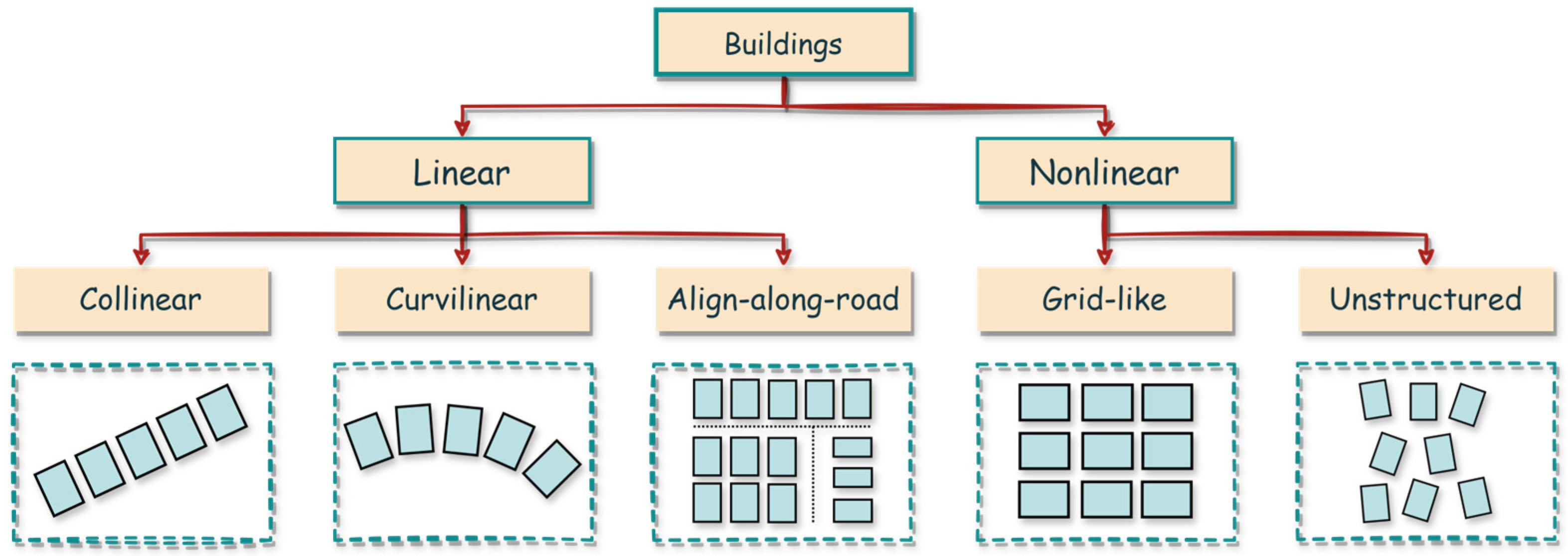
In spatial networks, buildings form an interconnected and interdependent topological structure, commonly referred to in spatial cognition research as the spatial distribution pattern of spatial objects. Such patterns typically exhibit significant spatial autocorrelation, which may manifest in either linear or nonlinear forms (Figure 7).
Traditional first-order neighborhood aggregation ( k = 1 ) in GAT considers only directly adjacent buildings, making it insufficient for fully modeling this spatial dependency. To address this limitation, we adopt second-order neighborhood aggregation ( k = 2 ) , enabling feature propagation to second-order neighbors via a message-passing mechanism. Specifically, two sequential GAT computations are performed: the first computes features for direct neighbors, and the second aggregates from neighbors that have already undergone one round of feature update.
The attention computation for the first-order and second-order neighbors in head k is expressed as:
e i j k = L e a k y R e L U a 1 k W 1 k h i l 1   | |   W 1 k h j l 1 ,   a i j = s o f t m a x e i j k
e i k k = L e a k y R e L U a 2 k W 2 k h i l 1   | |   W 2 k h k l 1 ,   a i j = s o f t m a x e i k k
where a 1 k and a 2 k are the learnable attention parameters for head k , and W 1 k and W 2 k are the corresponding feature transformation matrices.
Incorporating multi-head attention, the aggregation function is formulated as:
h i ( l ) = | | k = 1 K σ ( j ϵ N i ( i ) α i j k W 1 k h j ( l 1 ) + β k ϵ N 2 ( i ) γ i k k W 2 k h k ( l 1 ) )
where | | denotes vector concatenation, producing an output dimension of K × F , with F being the dimension after transformation by W . β is a learnable coefficient controlling the strength of second-order aggregation (initialized at 0.5), and σ is a non-linear activation function. The schematic diagram of second-order neighborhood aggregation is shown in Figure 8.
Although higher-order aggregation (e.g., third-order) is theoretically possible, in practice it tends to cause overfitting and oversmoothing in clustering tasks.

3.4.3. Distance-Constrained Attention Mechanism

Tobler’s First Law of Geography—“Everything is related to everything else, but near things are more related than distant things”—captures the essence of spatial autocorrelation, i.e., the correlation of geographic phenomena decreases with increasing distance. In light of this principle, we embed an exponential distance decay term g into the standard GAT attention mechanism, making the attention weight decay with distance:
g = e x p ( γ d i j )
where γ > 0 is a learnable decay coefficient. A larger γ results in faster decay (emphasizing closer neighbors), whereas a smaller γ yields a gentler decay (allowing farther buildings to contribute).
The distance bias term reflects the strength of spatial correlation: in dense urban cores, γ should be relatively large; in sparsely built suburban areas, γ should be smaller.
The improved attention coefficient calculation formula is obtained by introducing Equation (16) into Equation (10):
a i j = e x p ( L e a k y R e L U a h i   | |   h j g ) k N ( i ) e x p ( L e a k y R e L U ( a [ h i   | |   h j ] ) g )

3.5. Clustering Result Generation and Evaluation

3.5.1. Spectral Clustering

Spectral clustering is a widely used clustering algorithm originating from graph theory, which has since found extensive application in data clustering [52,53,54]. Compared to traditional clustering approaches, spectral clustering exhibits stronger adaptability to complex data distributions, often delivers superior clustering performance, and maintains relatively low computational complexity. Moreover, its implementation is straightforward.
The core idea is to regard all data samples as nodes in a space, where edges between nodes are weighted by their similarity: two distant nodes have a low edge weight, while two close nodes have a high edge weight. Consequently, the clustering problem is transformed into a graph partitioning problem, aiming to maximize the total edge weight within clusters while minimizing the weight between clusters.
To perform spectral clustering, a graph structure is first constructed from the dataset. Common methods include the Delaunay triangulation, minimum spanning tree (MST), and k-nearest neighbor (KNN) graph. Among these, the Delaunay triangulation exhibits strong neighborhood detection capabilities, making it particularly suitable for modeling building spatial relationships. In this study, spectral clustering is applied to the similarity matrix output from the GAT, following these steps:
  • Step 1: Compute the degree matrix D , a diagonal matrix whose diagonal elements are the row sums of the similarity matrix S i j :
    D = j = 1 n S i j
  • Step 2: Construct the normalized Laplacian matrix in its symmetric form:
    L s y m = D 1 / 2 D S D 1 / 2
    where D 1 / 2 is a diagonal matrix with elements D i i 1 / 2 .
  • Step 3: Perform eigen-decomposition on L s y m to obtain the first k eigenvectors corresponding to its smallest eigenvalues: u 1 , u 2 , , u k . Form the matrix U S n k whose columns are the eigenvectors:
    U = u 1 , u 2 , , u k
    Normalize each row of U to unit length ( L 2 normalization) to obtain matrix T :
    T i j = U i j l = 1 k U i l 2
  • Step 4: Treat each row of T as a point in S n k and perform K-means clustering to produce the final partition:
    C l u s t e r i = K m e a n s T i : ,   i = 1,2 , , n
In addition, for determining the number of clusters, this paper employs the elbow method. This method requires calculating the sum of squared errors (SSE) between each point and its corresponding cluster centroid for each number of clusters. The SSE is computed as follows:
S S E =   i = 1 k j C i j μ i 2
where μ is the centroid of the i-th cluster, and j is a data point belonging to the i -th cluster. Not all points are compared to all cluster centroids, otherwise, the SSE would not approach 0 as the number of clusters increases. Since the SSE decreases and approaches 0 as the number of clusters grows, there will be a segment where the rate of decrease is steep, and as the number of clusters continues to increase, the rate of decrease will stabilize. Therefore, we typically select the endpoint of the steepest decline segment as the true number of clusters [37].
By applying spectral clustering to the learned similarity matrix from the GAT, the algorithm leverages both the multi-feature fusion and spatial constraints captured during graph attention learning, resulting in building clusters that exhibit high semantic coherence and strong spatial continuity.

3.5.2. Design of Clustering Evaluation Metrics

Since spectral clustering is an unsupervised learning method, conventional supervised performance metrics—such as accuracy and precision—cannot be directly applied. This makes the objective evaluation of clustering quality more challenging. In this study, we adopt three representative metrics: Cluster Compactness, Silhouette Coefficient, and Adjusted Rand Index (ARI) [6,55,56,57,58]. Compactness serves as an indicator of within-cluster spatial cohesion. A lower Compactness value indicates that the feature similarity among buildings within the same cluster is more concentrated and continuous, corresponding to less fragmentation and clearer block-like urban structures. Because this metric does not directly reflect inter-cluster separation or cluster-shape complexity, we also use the silhouette coefficient, which considers each sample’s distance to its own cluster and to the nearest other cluster; higher values indicate stronger internal cohesion and greater external separation, thereby compensating for Compactness’s insensitivity to between-cluster separation. Finally, we use the ARI to measure the agreement between the clustering results and the ground-truth labels.
1.
Cluster Compactness
Compactness measures the degree of similarity aggregation within a cluster, with smaller values indicating higher intra-cluster cohesion [54]. Based on the similarity matrix S , it is computed as:
C o m p a c t n e s s k = 1 C k 2 i , j C k ( 1 S i j )
where C k denotes the set of buildings in the k -th cluster, and S i j [ 0,1 ] represents the similarity between buildings i and j . This metric directly reflects the clustering model’s ability to group similar buildings closely together.
2.
Silhouette Coefficient
The Silhouette Coefficient jointly evaluates intra-cluster cohesion and inter-cluster separation [59], and is defined as:
s ( i ) = b i a ( i ) m a x { a i , b ( i ) }
where a ( i ) is the average distance between sample i and all other samples in the same cluster, and b i is the minimum average distance between i and all samples in any other cluster. The coefficient ranges from [ 1,1 ] : values close to 1 indicate well-clustered samples, values near 0 suggest boundary points between clusters, and negative values imply possible misclassification. The mean silhouette score across all samples is used as the overall clustering quality indicator.
3.
Adjusted Rand Index (ARI)
The ARI measures the agreement between predicted clusters and ground-truth labels, adjusting for chance grouping [60]. It is defined as:
A R I = R I R I e x p e c t e d max R I R I e x p e c t e d , R I = a + b a + b + c + d
where a is the number of pairs in the same cluster in both true and predicted partitions; b is the number of pairs in the same true cluster but in different predicted clusters; c is the number of pairs in different true clusters but in the same predicted cluster; and d is the number of pairs in different clusters in both partitions.
The expected Rand Index R I e x p e c t e d for random assignments is computed as:
R I e x p e c t e d = n 2 + i n i 2 j n j 2 2 i , j n i j 2 n 2 2
where n is the total number of samples, n i is the number of samples in class i in the true labels, n i is the number of samples in predicted cluster j , and n i j is the number of samples assigned to both class i and predicted cluster j . The ARI ranges from [ 1,1 ] , with higher values indicating greater similarity between the predicted and true partitions.

4. Results

4.1. Data Collection and Analysis

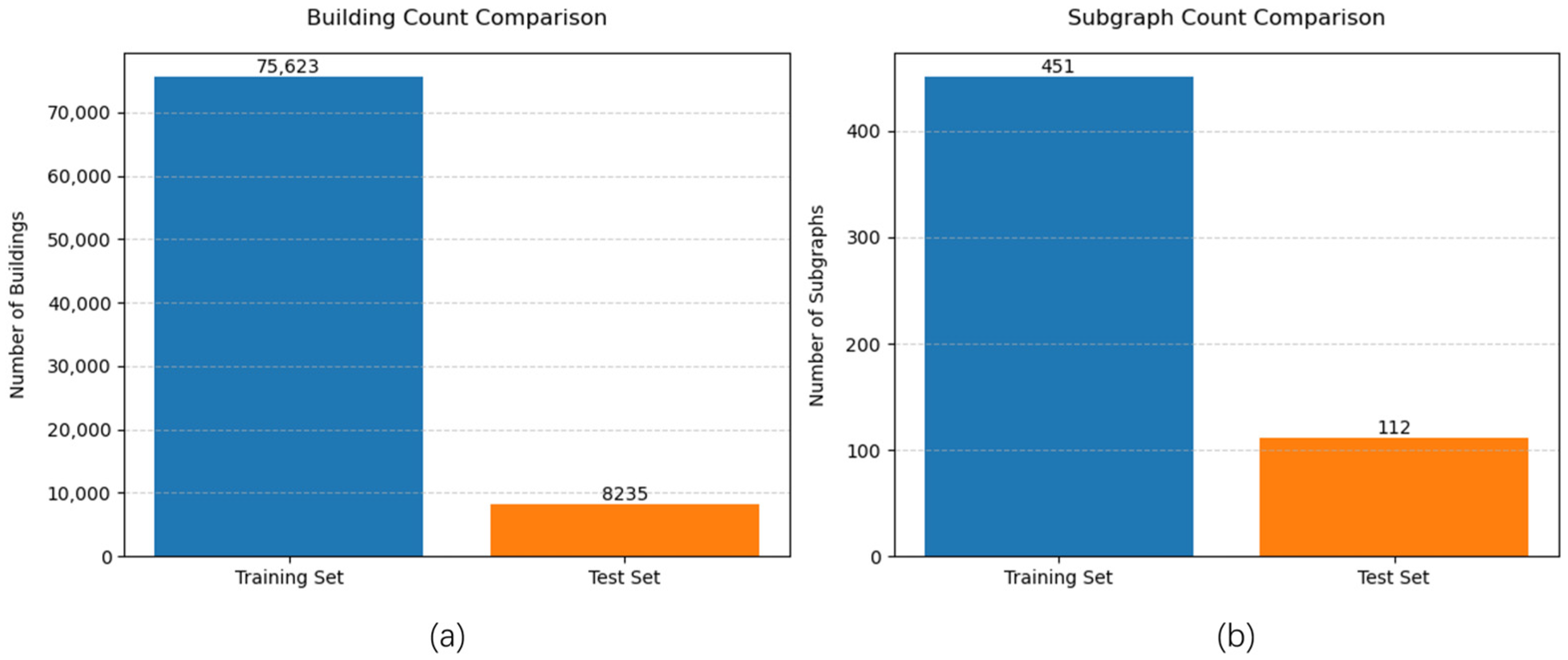
The experimental study area covers two Chinese cities—Xi’an and Beijing. Building footprint data were obtained from the publicly available OpenStreetMap (OSM) dataset, while building color features were extracted from GF-2 satellite imagery. The dataset was split into training and testing sets at an 8:2 ratio, based on subdivision by the primary road network. The training set contains 451 subgraphs with 75,623 buildings, while the testing set includes 112 subgraphs with 8235 buildings (Figure 9).
Three representative regions were selected for evaluation:
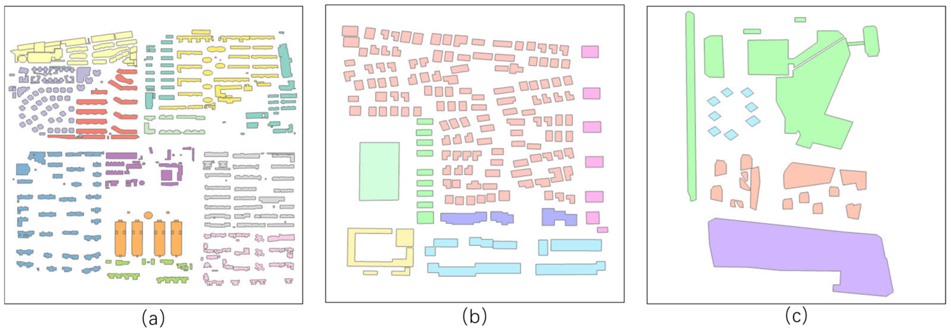
  • Region 1: Qujiang New District, Xi’an (34.1990° N, 108.9595° E to 34.1893° N, 108.9704° E)—369 buildings, dense commercial zone.
  • Region 2: Residential area near Beijing Normal University High School, Daxing District, Beijing (39.7759° N, 116.3164° E to 39.7717° N, 116.3212° E)—168 buildings, medium-density residential area.
  • Region 3: Huiju Shopping Mall area, Xihongmen, Daxing District, Beijing (39.79002° N, 116.3142°E to 39.77836° N, 116.3246° E)—31 buildings, low-density irregular distribution.
These regions represent three typical patterns in urban building clustering: high-density regular, medium-density regular, and low-density irregular.
As a comparison for the experiment, we classified buildings in the three study areas manually, with the classification labels shown in Figure 10.

4.2. LA-GATs Clustering Results

The proposed LA-GATs model employs three attention layers with four attention heads each to improve prediction accuracy and stability. The Adam optimizer was used with a learning rate of 0.001, and training was performed for 2500 iterations. The Adam optimizer adapts the learning rate for each parameter, which is particularly effective for optimizing complex Graph Attention Networks (GATs) [14,61,62,63]. A learning rate of 0.001 was selected based on its effectiveness in similar deep learning tasks, providing stable convergence without causing oscillation or slow convergence. The loss function was categorical cross-entropy, optimized via backpropagation.
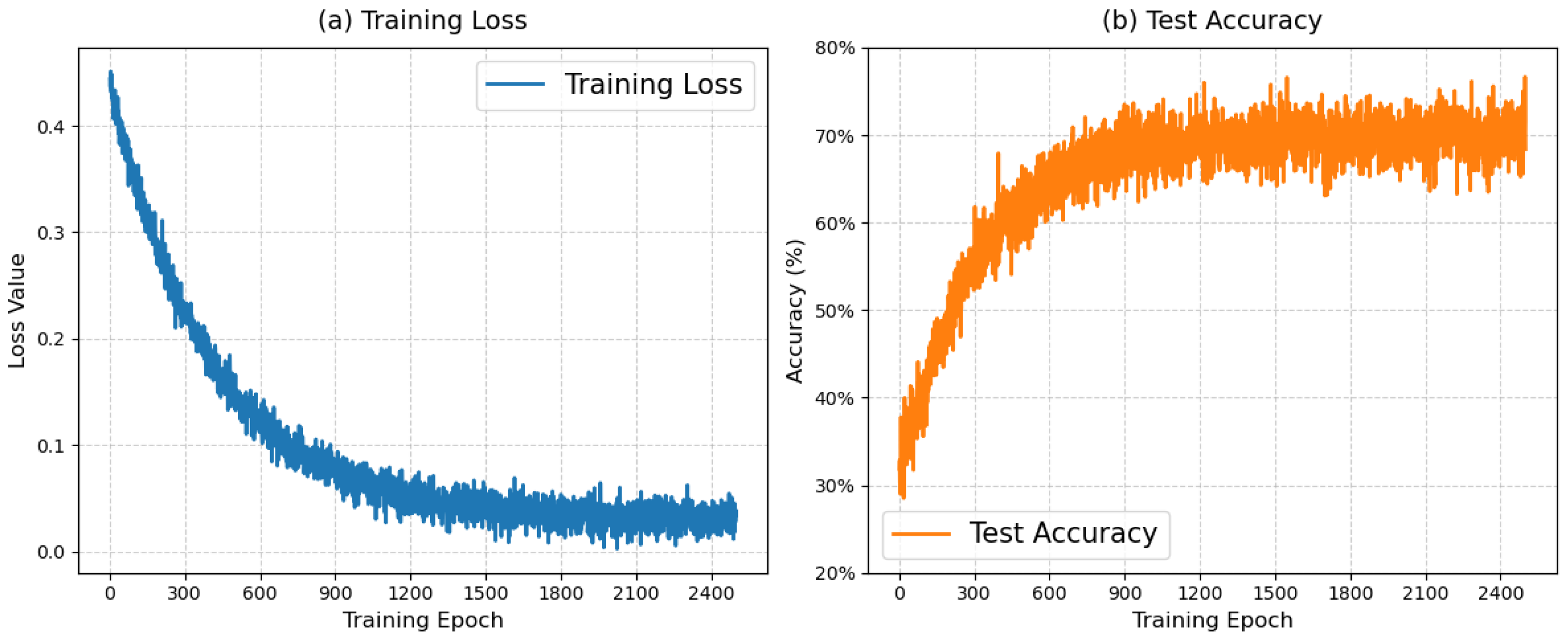
The training accuracy and loss curves are shown in Figure 11, demonstrating smooth convergence with final accuracy exceeding 95% and stable low loss, indicating effective model optimization.
For the three test regions, the clustering accuracy against manual annotations reached 65.5%, 71.2%, and 75.1% for Regions 1–3, respectively, visually confirming alignment with human perception of spatial building distribution.

4.3. Component Contribution Analysis

To evaluate the contributions of the distance bias term and the second-order neighborhood aggregation in the LA-GATs model, two groups of comparative experiments were conducted. The comparison was carried out on three representative study areas: Test1 (high-density regular), Test2 (medium-density regular), and Test3 (low-density irregular). The evaluation metrics include Compactness, Adjusted Rand Index (ARI), and Silhouette Coefficient.

4.3.1. Impact of Distance Bias Term

In the first set of comparative experiments, the distance bias term ( γ 0 ) in the graph attention mechanism was removed ( γ = 0 ) while keeping all other parameters unchanged. Table 1 reports the clustering performance in all three study areas with and without the distance bias term.
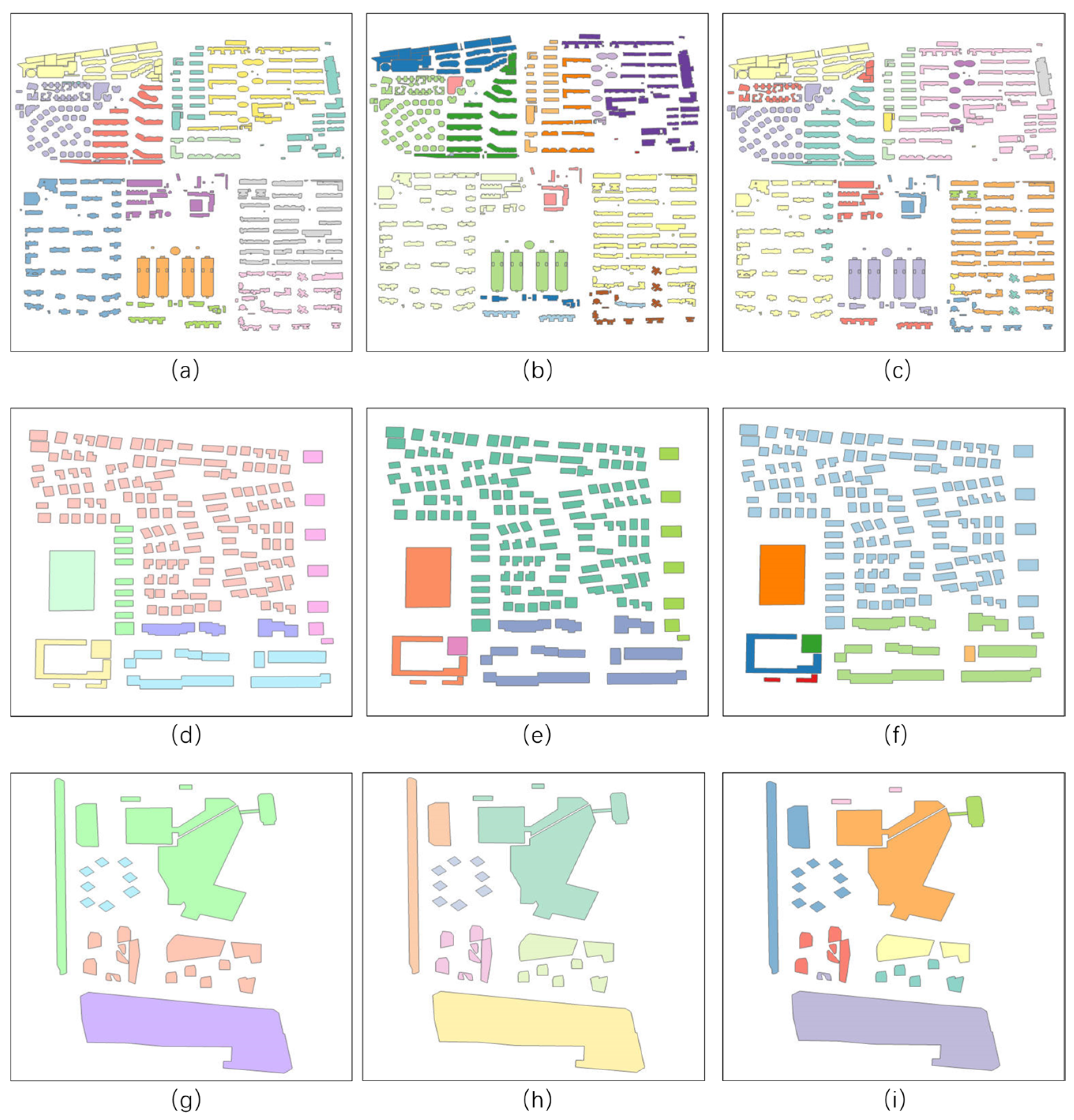
As shown in Figure 12, removing the distance bias term leads to significant performance degradation across all three metrics, with ARI dropping by an average of 15%, Compactness increasing by 28% (lower is better), and the Silhouette Coefficient decreasing by 25% on average. This demonstrates that the distance bias term plays a critical role in maintaining spatial continuity and preventing over-segmentation in the clustering process.

4.3.2. Impact of Second-Order Neighborhood Aggregation

The second set of comparative experiments compared first-order neighborhood aggregation ( k = 1 ) with second-order neighborhood aggregation ( k = 2 ) . Table 2 presents the results.
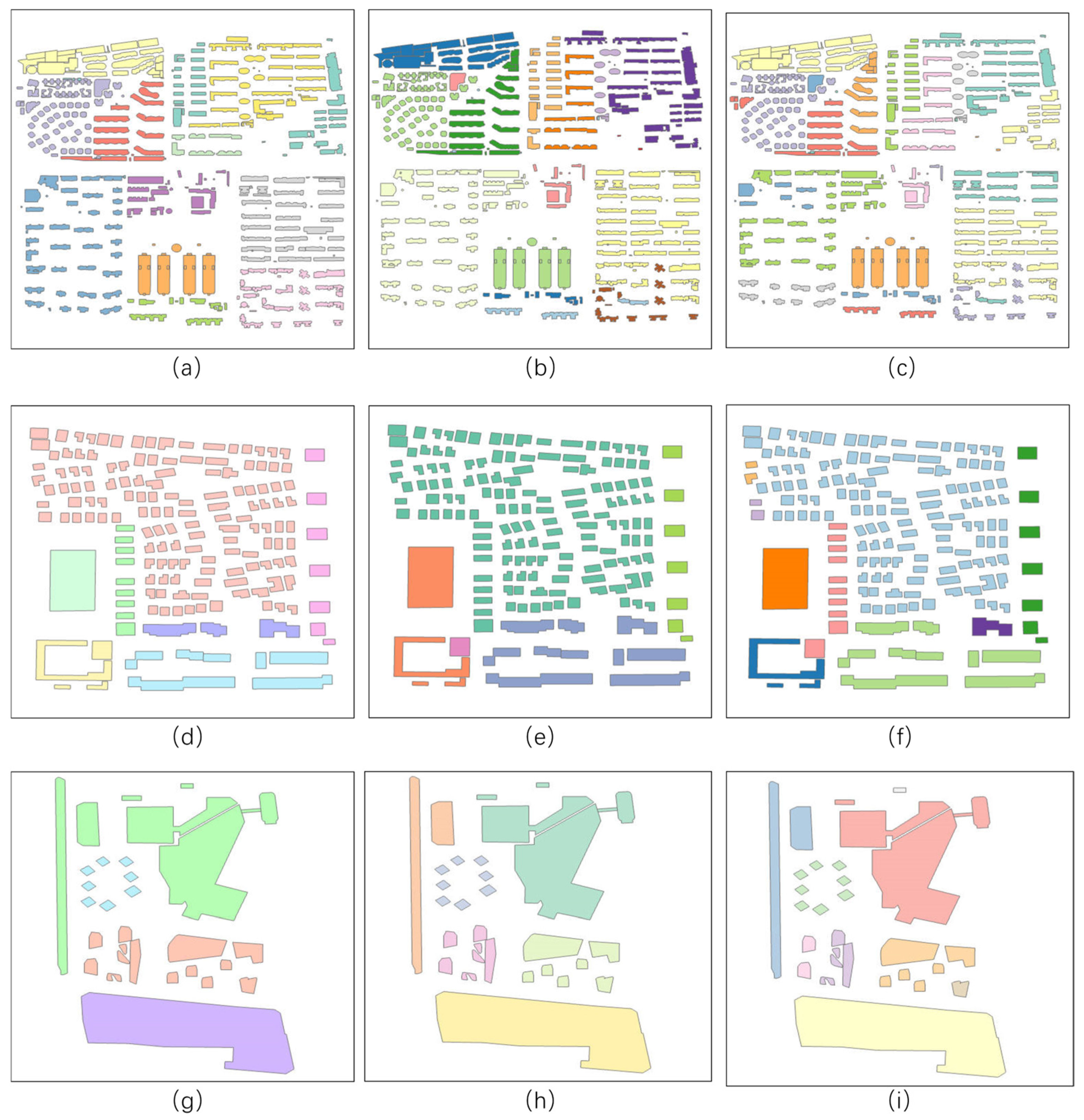
As shown in Figure 13, compared with first-order aggregation, second-order neighborhood aggregation shows consistent improvements in ARI and Silhouette Coefficient across all study areas, with the most significant gains observed in Test 2 (medium-density residential area). This confirms that second-order aggregation captures broader contextual information and alleviates local over-segmentation.

4.4. Comparison with Multiple Clustering Algorithms

To further validate the effectiveness of LA-GATs, we benchmark it against four clustering methods. DBSCAN and k-means serve as classical unsupervised baselines; a minimum-spanning-tree (MST) method represents a purely graph-theoretic approach; and Graph Attention Networks (GATs) provide a graph-based deep learning baseline. All experiments were conducted under identical parameter settings, and all methods were evaluated using the same metrics.
As shown in Table 3, LA-GATs outperforms other methods across all metrics in the test areas, with particularly notable gains in ARI, in which LA-GATs improves over K-means by more than 150%. Furthermore, LA-GATs achieves higher Silhouette Coefficients, indicating a better balance between intra-cluster compactness and inter-cluster separation (Figure 14).

5. Conclusions

This study proposes a building clustering method based on an improved Graph Attention Network (LA-GATs), which integrates a distance-aware attention mechanism and a second-order neighborhood aggregation strategy to overcome the limitations of conventional approaches in recognizing spatial distribution patterns of buildings. The main innovations and contributions are as follows:
  • Extension and optimization of GATs-based building clustering—enhancing the model architecture to better capture spatial and semantic relationships among buildings.
  • Incorporation of spatially constrained attention—introducing a distance bias term to explicitly model spatial autocorrelation. Experiments conducted in Xi’an and Beijing show notable improvements in clustering evaluation metrics with this mechanism.
  • Adaptive second-order neighborhood aggregation strategy—expanding the receptive field of feature propagation to improve the recognition of building group patterns. The ARI value reflects the consistency between clustering results and true labels, serving as an accuracy metric for clustering outcomes [55,56]. This strategy improves clustering accuracy by approximately 21% over existing clustering methods in residential areas, while maintaining the separability of distinct functional zones.
Experimental results across three representative test areas demonstrate that LA-GATs significantly outperforms traditional clustering methods (DBSCAN and K-means), particularly in high-density commercial zones and heterogeneous residential areas. The Compactness and ARI metrics further validate the model’s advantage in preserving both spatial continuity and semantic coherence.
Despite these promising results, several avenues remain for further exploration:
  • The current methods primarily focus on the features of each building; future work could incorporate block-level or city-scale contextual information to enhance the recognition of complex spatial patterns.
  • The methodology proposed in this study is designed primarily for typical urban built environments, including residential, commercial, and mixed-use areas. In environments with distinctive architectural characteristics (e.g., contiguous historic districts/ancient architectural complexes), material distribution, color application, and structural forms may exhibit significant deviations from conventional urban textures. Expanding the number of building features, feature calculation methods, or feature categories (semantically related features) can optimize GATs training outcomes. We identify this as a priority topic for future research.
  • The integration of advanced machine learning architectures such as Transformer and LSTM could further refine the attention mechanism, enabling improved building clustering and citywide spatial distribution prediction.

Author Contributions

Conceptualization, Xincheng Yang, Xukang Xie and Dingming Liu; Methodology, Xincheng Yang and Xukang Xie; Software, Xincheng Yang and Dingming Liu; Validation, Xukang Xie; Formal analysis, Xukang Xie; Investigation, Xincheng Yang and Xukang Xie; Resources, Dingming Liu; Data curation, Xukang Xie; Writing–original draft, Xincheng Yang; Writing–review & editing, Xincheng Yang; Visualization, Xincheng Yang; Supervision, Xukang Xie; Project administration, Dingming Liu; Funding acquisition, Xincheng Yang. All authors have read and agreed to the published version of the manuscript.

Funding

This research received no external funding.

Data Availability Statement

The original contributions presented in the study are included in the article. The data used in this study is publicly available from OpenStreetMap (OSM) open-source data. However, the code used for analysis is not publicly available. Further inquiries regarding the data or study can be directed to the corresponding author.

Acknowledgments

The authors are grateful to Xukang Xie for his contribution to resources and investigation of this article.

Conflicts of Interest

Authors Xincheng Yang and Dingming Liu were employed by the company Aerial Photogrammetry and Remote Sensing Group Co., Ltd. The remaining authors declare that the research was conducted in the absence of any commercial or financial relationships that could be construed as a potential conflict of interest.

References

  1. Yu, W.; Ai, T.; Liu, P.; Cheng, X. The Analysis and Measurement of Building Patterns Using Texton Co-Occurrence Matrices. Int. J. Geogr. Inf. Sci. 2017, 31, 1079–1100. [Google Scholar] [CrossRef]
  2. He, X.; Deng, M.; Luo, G. Recognizing Building Group Patterns in Topographic Maps by Integrating Building Functional and Geometric Information. ISPRS Int. J. Geo-Inf. 2022, 11, 332. [Google Scholar] [CrossRef]
  3. Yan, X.; Ai, T.; Zhang, X. Template Matching and Simplification Method for Building Features Based on Shape Cognition. ISPRS Int. J. Geo-Inf. 2017, 6, 250. [Google Scholar] [CrossRef]
  4. Xing, R.; Wu, F.; Gong, X.; Du, J.; Liu, C. An Axis-Matching Approach to Combined Collinear Pattern Recognition for Urban Building Groups. Geocarto Int. 2022, 37, 4823–4842. [Google Scholar] [CrossRef]
  5. Hu, Y.; Liu, C.; Li, Z.; Xu, J.; Han, Z.; Guo, J. Few-Shot Building Footprint Shape Classification with Relation Network. ISPRS Int. J. Geo-Inf. 2022, 11, 311. [Google Scholar] [CrossRef]
  6. Chen, G.; Qian, H. Building clustering method that integrates graph attention networks and spectral clustering. Geocarto Int. 2025, 40, 2471091. [Google Scholar] [CrossRef]
  7. Deng, M.; Tang, J.; Liu, Q.; Wu, F. Recognizing building groups for generalization: A comparative study. Cartogr. Geogr. Inf. Sci. 2018, 45, 187–204. [Google Scholar] [CrossRef]
  8. Li, Z.; Yan, H.; Ai, T.; Chen, J. Automated building generalization based on urban morphology and Gestalt theory. Int. J. Geogr. Inf. Sci. 2004, 18, 513–534. [Google Scholar] [CrossRef]
  9. Ai, T.; Guo, R. Polygon cluster pattern mining based on gestalt principles. Acta Geod Cart. Sin. 2007, 36, 302–308. [Google Scholar]
  10. Liu, H.; Wang, W.; Tang, J.; Deng, M.; Ding, C. A Building Group Recognition Method Integrating Spatial and Semantic Similarity. ISPRS Int. J. Geo-Inf. 2025, 14, 154. [Google Scholar] [CrossRef]
  11. Qi, H.B.; Li, Z.L. An Approach to Building Grouping Based on Hierarchical Constraints. Int. Arch. Photogramm. Remote Sens. Spat. Inf. Sci. 2008, 2008, 449–454. [Google Scholar]
  12. Boffet, A.; Serra, S.R. Identification of spatial structures within urban blocks for town characterization. In Proceedings of the 20th International Cartographic Conference, Beijing, China, 6–10 August 2001; Volume 3, pp. 1974–1983. [Google Scholar]
  13. Ezugwu, A.E.; Ikotun, A.M.; Oyelade, O.O.; Abualigah, L.; Agushaka, J.O.; Eke, C.I.; Akinyelu, A.A. A comprehensive survey of clustering algorithms: State-of-the-art machine learning applications, taxonomy, challenges, and future research prospects. Eng. Appl. Artif. Intell. 2022, 110, 104743. [Google Scholar] [CrossRef]
  14. Vaswani, A.; Shazeer, N.; Parmar, N.; Uszkoreit, J.; Jones, L.; Gomez, A.N.; Kaiser, Ł.; Polosukhin, I. Attention is all you need. Adv. Neural Inf. Process. Syst. 2017, 30, 5998–6008. [Google Scholar] [CrossRef]
  15. Veličković, P.; Cucurull, G.; Casanova, A.; Romero, A.; Lio, P.; Bengio, Y. Graph attention networks. arXiv 2017, arXiv:1710.10903. [Google Scholar] [CrossRef]
  16. Liu, P.; Shao, Z.; Xiao, T. Second-order texton feature extraction and pattern recognition of building polygon cluster using CNN network. Int. J. Appl. Earth Obs. Geoinf. 2024, 129, 103794. [Google Scholar] [CrossRef]
  17. Gao, A.; Lin, J. ConstellationNet: Reinventing Spatial Clustering through GNNs. arXiv 2025, arXiv:2503.07643. [Google Scholar] [CrossRef]
  18. Tsitsulin, A.; Palowitch, J.; Perozzi, B.; Müller, E. Graph clustering with graph neural networks. J. Mach. Learn. Res. 2023, 24, 1–21. [Google Scholar]
  19. Kong, B.; Ai, T.; Zou, X.; Yan, X.; Yang, M. A graph-based neural network approach to integrate multi-source data for urban building function classification. Comput. Environ. Urban Syst. 2024, 110, 102094. [Google Scholar] [CrossRef]
  20. Ai, T.; Liu, Y. A method of point cluster simplification with spatial distribution properties preserved. Acta Geod Cart. Sin. 2002, 31, 175–181. [Google Scholar]
  21. Rodriguez, A.; Laio, A. Clustering by fast search and find of density peaks. Science 2014, 344, 1492–1496. [Google Scholar] [CrossRef]
  22. Huimin, L.I.U.; Wenke, H.U.; Jianbo, T.A.N.G.; Yan, S.H.I.; Min, D.E.N.G. A method for recognizing building clusters by considering functional features of buildings. Acta Geod. Cartogr. Sin. 2020, 49, 622. [Google Scholar]
  23. Jin, C.; An, X.; Chen, Z.; Ma, X. A multi-level graph partition clustering method of vector residential area polygon. Geomat. Inf. Sci. Wuhan Univ. 2021, 46, 19–29. [Google Scholar]
  24. Yan, H.; Weibel, R.; Yang, B. A multi-parameter approach to automated building grouping and generalization. Geoinformatica 2008, 12, 73–89. [Google Scholar] [CrossRef]
  25. Gao, X.; Yan, H.; Lu, X. Semantic similarity measurement for building polygon aggregation in multi-scale map space. Acta Geod. Cartogr. Sin. 2022, 51, 95. [Google Scholar]
  26. Regnauld, N. Contextual building typification in automated map generalization. Algorithmica 2001, 30, 312–333. [Google Scholar] [CrossRef]
  27. Regnauld, N. Spatial structures to support automatic generalization. In Proceedings of the XXII Int. Cartographic Conference, A Coruña, Spain, 9–16 July 2005. [Google Scholar]
  28. Sun, D.; Shen, T.; Yang, X.; Huo, L.; Kong, F. Research on a Multi-Scale Clustering Method for Buildings Taking into Account Visual Cognition. Buildings 2024, 14, 3310. [Google Scholar] [CrossRef]
  29. Von Luxburg, U. A tutorial on spectral clustering. Stat. Comput. 2007, 17, 395–416. [Google Scholar] [CrossRef]
  30. Paatero, P.; Tapper, U. Positive matrix factorization: A non-negative factor model with optimal utilization of error estimates of data values. Environmetrics 1994, 5, 111–126. [Google Scholar] [CrossRef]
  31. He, Z.; Xie, S.; Zdunek, R.; Zhou, G.; Cichocki, A. Symmetric nonnegative matrix factorization: Algorithms and applications to probabilistic clustering. IEEE Trans. Neural Netw. 2011, 22, 2117–2131. [Google Scholar] [CrossRef]
  32. Tang, F.; Wang, C.; Su, J.; Wang, Y. Spectral clustering-based community detection using graph distance and node attributes. Comput. Stat. 2020, 35, 69–94. [Google Scholar] [CrossRef]
  33. Zhang, X.; Liu, H.; Wu, X.-M.; Zhang, X.; Liu, X. Spectral embedding network for attributed graph clustering. Neural Netw. 2021, 142, 388–396. [Google Scholar] [CrossRef]
  34. Kang, Z.; Lin, Z.; Zhu, X.; Xu, W. Structured graph learning for scalable subspace clustering: From single view to multiview. IEEE Trans. Cybern. 2021, 52, 8976–8986. [Google Scholar] [CrossRef]
  35. Berahmand, K.; Mohammadi, M.; Faroughi, A.; Mohammadiani, R.P. A novel method of spectral clustering in attributed networks by constructing parameter-free affinity matrix. Clust. Comput. 2022, 25, 869–888. [Google Scholar] [CrossRef]
  36. Yan, X.; Ai, T.; Yang, M.; Tong, X.; Liu, Q. A graph deep learning approach for urban building grouping. Geocarto Int. 2022, 37, 2944–2966. [Google Scholar] [CrossRef]
  37. Shi, C.; Wei, B.; Wei, S.; Wang, W.; Liu, H.; Liu, J. A quantitative discriminant method of elbow point for the optimal number of clusters in clustering algorithm. EURASIP J. Wirel. Commun. Netw. 2021, 2021, 31. [Google Scholar] [CrossRef]
  38. Köhler, W. Gestalt psychology. Psychol. Forsch. 1967, 31, XVIII–XXX. [Google Scholar] [CrossRef] [PubMed]
  39. Zhang, L.; Wang, G.; Sun, W. Automatic extraction of building geometries based on centroid clustering and contour analysis on oblique images taken by unmanned aerial vehicles. Int. J. Geogr. Inf. Sci. 2022, 36, 453–475. [Google Scholar] [CrossRef]
  40. Duchêne, C.; Bard, S.; Barillot, X.; Ruas, A.; Trevisan, J.; Holzapfel, F. Quantitative and qualitative description of building orientation. In Proceedings of the Fifth Workshop on Progress in Automated Map Generalisation, Paris, France, 28–30 April 2003. [Google Scholar]
  41. Zhang, X.; Ai, T.; Stoter, J. Characterization and detection of building patterns in cartographic data: Two algorithms. In Advances in Spatial Data Handling and GIS: 14th International Symposium on Spatial Data Handling; Springer: Berlin/Heidelberg, Germany, 2012; pp. 93–107. [Google Scholar]
  42. Shirowzhan, S.; Lim, S.; Trinder, J.; Li, H.; Sepasgozar, S. Data mining for recognition of spatial distribution patterns of building heights using airborne lidar data. Adv. Eng. Inform. 2020, 43, 101033. [Google Scholar] [CrossRef]
  43. Yang, X.; Huo, L.; Shen, T.; Wang, X.; Yuan, S.; Liu, X. A large-scale urban 3D model organisation method considering spatial distribution of buildings. IET Smart Cities 2023, 6, 54–64. [Google Scholar] [CrossRef]
  44. Li, X.; Qin, C.; Qian, Z.; Yao, H.; Zhang, X. Perceptual Robust Hashing for Color Images with Canonical Correlation Analysis. arXiv 2020, arXiv:2012.04312. [Google Scholar] [CrossRef]
  45. Singh, A.; Khan, M.Z.; Sharma, S.; Debnath, N.C. Perceptual Hashing Algorithms for Image Recognition. In Proceedings of the International Conference on Advanced Intelligent Systems and Informatics, Port Said, Egypt, 20–22 January 2025; Springer Nature: Cham, Switzerland, 2025; pp. 90–101. [Google Scholar]
  46. Caruso, G.; Hilal, M.; Thomas, I. Measuring urban forms from inter-building distances: Combining MST graphs with a Local Index of Spatial Association. Landsc. Urban Plan. 2017, 163, 80–89. [Google Scholar] [CrossRef]
  47. Cetinkaya, S.; Basaraner, M.; Burghardt, D. Proximity-based grouping of buildings in urban blocks: A comparison of four algorithms. Geocarto Int. 2015, 30, 618–632. [Google Scholar] [CrossRef]
  48. Li, X.; Li, W.; Meng, Q.; Zhang, C.; Jancso, T.; Wu, K. Modelling building proximity to greenery in a three-dimensional perspective using multi-source remotely sensed data. J. Spat. Sci. 2016, 61, 389–403. [Google Scholar] [CrossRef]
  49. Bose, P.; De Carufel, J.L.; Shaikhet, A.; Smid, M. Essential constraints of edge-constrained proximity graphs. In Workshop on Combinatorial Algorithms; Springer International Publishing: Cham, Switzerland, 2016; pp. 55–67. [Google Scholar]
  50. Niroumand-Jadidi, M.; Vitti, A. Reconstruction of river boundaries at sub-pixel resolution: Estimation and spatial allocation of water fractions. ISPRS Int. J. Geo-Inf. 2017, 6, 383. [Google Scholar] [CrossRef]
  51. Maas, A.L.; Hannun, A.Y.; Ng, A.Y. Rectifier nonlinearities improve neural network acoustic models. Proc. icml. 2013, 30, 3. [Google Scholar]
  52. Zhou, J.; Du, Y.; Zhang, R.; Zhang, R. Adaptive depth graph attention networks. arXiv 2023, arXiv:2301.06265. [Google Scholar] [CrossRef]
  53. Chen, J.; Fang, C.; Zhang, X. Global attention-based graph neural networks for node classification. Neural Process. Lett. 2023, 55, 4127–4150. [Google Scholar] [CrossRef]
  54. Shi, J.; Malik, J. Normalized cuts and image segmentation. IEEE Trans. Pattern Anal. Mach. Intell. 2000, 22, 888–905. [Google Scholar] [CrossRef]
  55. Hassan, B.A.; Tayfor, N.B.; Hassan, A.A.; Ahmed, A.M.; Rashid, T.A.; Abdalla, N.N. From A-to-Z review of clustering validation indices. Neurocomputing 2024, 601, 128198. [Google Scholar] [CrossRef]
  56. Ikotun, A.M.; Habyarimana, F.; Ezugwu, A.E. Cluster validity indices for automatic clustering: A comprehensive review. Heliyon 2025, 11, e41953. [Google Scholar] [CrossRef]
  57. Zhang, T.; Lan, X.; Feng, J. A Progressive Clustering Approach for Buildings Using MST and SOM with Feature Factors. ISPRS Int. J. Geo-Inf. 2025, 14, 103. [Google Scholar] [CrossRef]
  58. Rousseeuw, P.J. Silhouettes: A graphical aid to the interpretation and validation of cluster analysis. J. Comput. Appl. Math. 1987, 20, 53–65. [Google Scholar] [CrossRef]
  59. Pavlopoulos, J.; Vardakas, G.; Likas, A. Revisiting silhouette aggregation. In International Conference on Discovery Science; Springer Nature: Cham, Switzerland, 2024; pp. 354–368. [Google Scholar]
  60. Hubert, L.; Arabie, P. Comparing partitions. J. Classif. 1985, 2, 193–218. [Google Scholar] [CrossRef]
  61. Xu, D.; Tian, Y. A comprehensive survey of clustering algorithms. Ann. Data Sci. 2015, 2, 165–193. [Google Scholar] [CrossRef]
  62. Kingma, D.P. Adam: A method for stochastic optimization. arXiv 2014, arXiv:1412.6980. [Google Scholar] [CrossRef]
  63. Zaheer, R.; Shaziya, H. A study of the optimization algorithms in deep learning. In Proceedings of the 2019 Third International Conference on Inventive Systems and Control (ICISC), Coimbatore, India, 10–11 January 2019; IEEE: New York, NY, USA, 2019; pp. 536–539. [Google Scholar] [CrossRef]
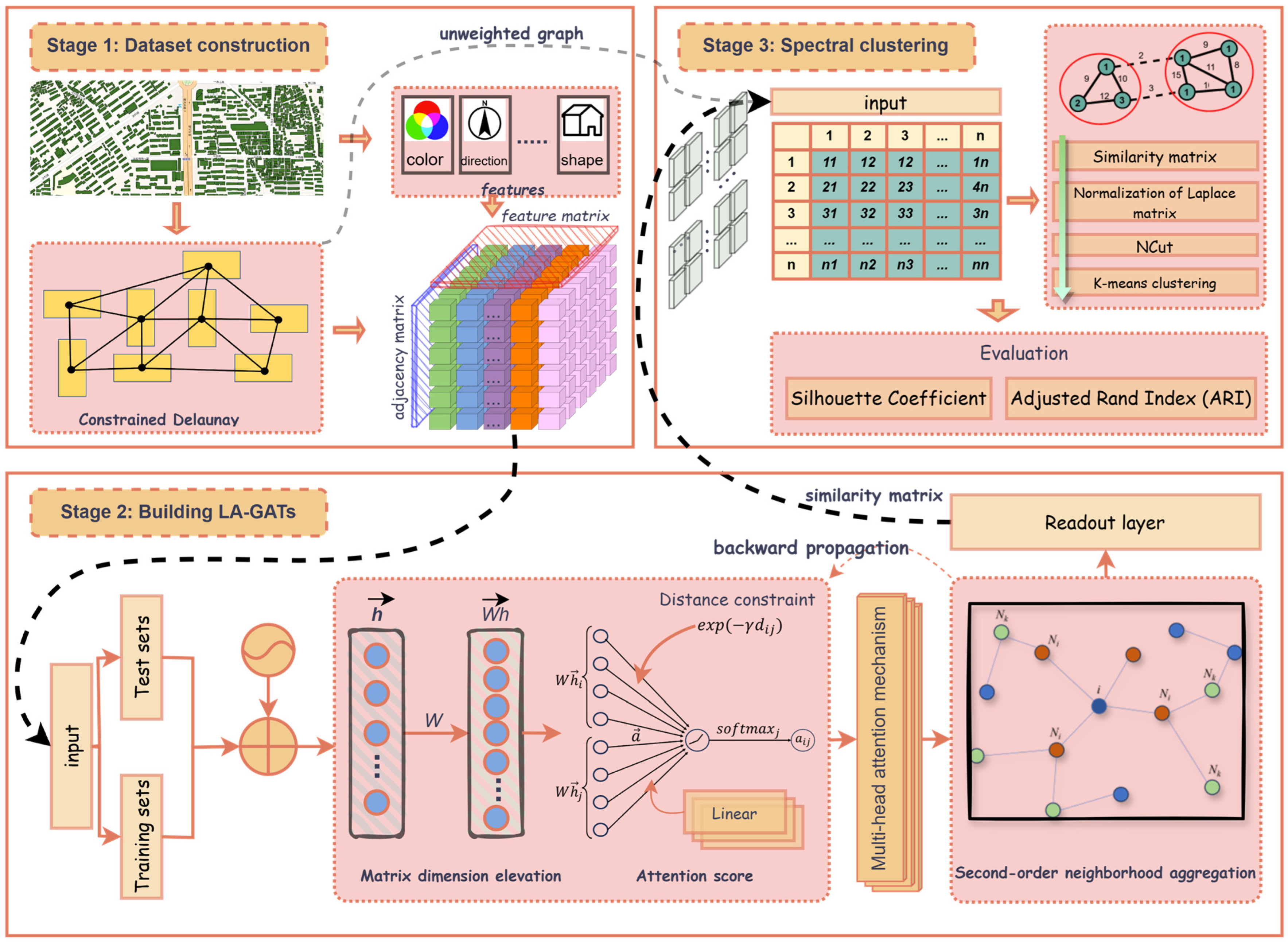
Figure 1. Pipeline of the proposed LA-GATs for building clustering.
Ijgi 14 00415 g001
Figure 2. Method for calculating the MBR direction: (a) The black rectangle represents the initial bounding rectangle of the building. (b) The process describes the adjustment of the bounding rectangle shape along the direction of the red arrow. (c) The area of the green bounding rectangle is the smallest among all bounding rectangles, and it is the minimum bounding rectangle (MBR). Its orientation corresponds to the direction of the building.
Ijgi 14 00415 g002
Figure 3. Comparison of constrained Delaunay triangulation before and after refinement. (a) is the Delaunay triangulation directly constructed based on the building vertices; (b) is the triangulation constructed after refinement using interpolation encryption.
Ijgi 14 00415 g003
Figure 4. Triangle classification and adjacency distance computation: (a) examples of the three classified triangle types; (b) result after removing Type 3 triangles; (c) Red lines indicate the Delaunay triangulation edges incident to the lower-left and lower-right buildings; these edges are used to compute the adjacency distance between the two buildings.
Ijgi 14 00415 g004
Figure 5. Schematic diagram of the nearest-neighbor graph construction.
Ijgi 14 00415 g005
Figure 6. Schematic diagram of the building proximity graph. i represents a building node in the GATs training; Ni represents the first-order neighboring nodes of node i; Nk represents the second-order neighboring nodes of node i.
Ijgi 14 00415 g006
Figure 7. Types of building distribution models.
Ijgi 14 00415 g007
Figure 8. Schematic diagram of second-order neighborhood aggregation.
Ijgi 14 00415 g008
Figure 9. (a) Building statistics for the training set and test set; (b) Quantitative statistics for the training set and test set.
Ijgi 14 00415 g009
Figure 10. Artificial clustering results; (a) Qujiang New District, Xi’an; (b) Residential area near Beijing Normal University High School, Daxing District, Beijing; (c) Huiju Shopping Mall area, Xihongmen, Daxing District, Beijing.
Ijgi 14 00415 g010
Figure 11. Distribution of model training set loss values and test set accuracy. (a) Training set loss values. (b) Test set accuracy.
Ijgi 14 00415 g011
Figure 12. Clustering results of the comparative experiment; (a,d,g) are the artificial clustering results of Test1, Test2, and Test3, respectively; (b,e,h) are the clustering results of Test1, Test2, and Test3 with distance bias terms, respectively; (c,f,i) are the clustering results of Test1, Test2, and Test3 without distance bias terms, respectively.
Ijgi 14 00415 g012
Figure 13. Clustering results of the comparative experiment; (a,d,g) are the artificial clustering results of Test1, Test2, and Test3, respectively; (b,e,h) are the clustering results of Test1, Test2, and Test3 after second-order neighborhood aggregation; (c,f,i) are the clustering results of Test1, Test2, and Test3 after first-order neighborhood aggregation.
Ijgi 14 00415 g013
Figure 14. Clustering results of the comparative experiment; (a) is the artificial clustering result/ground truth label for Test 1; (b) is the clustering result of the proposed method for Test 1; (c) is the GATs clustering result for Test 1; (d) is the MST clustering result for Test 1; (e) is the DBSCAN clustering result for Test 1; (f) is the K-means clustering result for Test 1.
Ijgi 14 00415 g014
Table 1. Clustering metric comparison table; γ = 0 is the metric without distance constraints; γ 0 is the metric after constraints are applied in this paper.
CompactnessARISilhouette
γ = 0 γ 0 γ = 0 γ 0 γ = 0 γ 0
Test10.2010.1530.720.870.520.65
Test20.2170.1590.750.890.500.67
Test30.2250.1610.780.920.480.69
Table 2. Clustering indicator comparison table; k = 1 is the indicator under first-order aggregation; k = 2 is the indicator under second-order aggregation in this paper.
CompactnessARISilhouette
k = 1 k = 2 k = 1 k = 2 k = 1 k = 2
Test10.1870.1530.790.870.580.65
Test20.1930.1590.810.890.600.67
Test30.2010.1610.860.920.620.69
Table 3. Clustering metric comparison table; comparison of metric parameters for LA-GATs, DBSCAN, and K-means clustering.
CompactnessARISilhouette
LA-GATs0.1530.870.65
GATs0.1770.690.61
MST0.2200.630.58
DBSCAN0.2520.620.52
K-means0.3540.280.41
Disclaimer/Publisher’s Note: The statements, opinions and data contained in all publications are solely those of the individual author(s) and contributor(s) and not of MDPI and/or the editor(s). MDPI and/or the editor(s) disclaim responsibility for any injury to people or property resulting from any ideas, methods, instructions or products referred to in the content.