A Risk Assessment Method of Three-Dimensional Low-Attitude Airspace Based on Multi-Source Data

Abstract

The safe operation of low-altitude UAVs is crucial for the effective utilization of low-altitude airspace, necessitating the development of appropriate risk assessment methods to evaluate the associated operational risks. However, current research primarily focuses on two-dimensional risk assessments, with limited focus on assessing risks across different heights, thus constraining the ability to guide UAV operations within three-dimensional airspace. In this study, we propose a three-dimensional airspace risk assessment method that integrates multisource data to estimate risks at various altitudes. First, we assess ground impact risks by considering factors such as population density, obstacle environment, and socioeconomic characteristics. Next, we develop a network signal evaluation model to estimate signal loss at various altitudes. Finally, we apply machine learning methods to classify multiple features to determine airspace risks at varying altitudes, resulting in a comprehensive three-dimensional risk map. The results indicate that the majority of the urban area falls within the low-risk category, accounting for approximately 84–87% of the city. High-risk regions are concentrated in central urban areas, with their proportion increasing from 5.9% at 30 m to 9.1% at 300 m. Although the overall trend remains broadly consistent across altitudes, the local variations highlight the necessity of three-dimensional risk evaluation. This three-dimensional risk map can effectively guide safe UAV operations across different altitude layers and provide valuable decision support for flight route planning.

1. Introduction

The large-scale utilization of low-altitude resources has become an important factor in promoting low-altitude economic development, and the concept of digital low-altitude ushering in a period of rapid growth, driven by advancements in the Internet of Every- thing [1]. The unmanned aerial vehicle (UAV) industry serves as a crucial pillar of low-altitude economic development, with a significant increase in UAV applications within urban environments [2,3].

To facilitate the rapid development of the UAV industry, it is crucial to ensure the flight safety of UAVs. Given that UAV flights occur predominantly in near-ground, low-altitude, and ultralow-altitude environments, the urban low-altitude environment is relatively complex and variable, posing significant challenges to the safe and efficient operation of UAVs [4]. The concept of flight risk has been developed to assess the safety of UAV operations. The Joint Authorities for the Rulemaking of Unmanned Systems initially clarified the concept of risk [5], defining it as a combination of the frequency (probability) of an event and its associated severity. They then proposed the specific operations risk assessment (SORA) method to assess both ground and air risks associated with UAV operations. Air risk refers to the hazards posed by the UAV during flight, influenced by the surrounding environment, other UAVs, or manned aircraft. Ground collision risk encompasses the potential harm to ground personnel and property in the event of an abnormal UAV crash, determined by parameters such as UAV mass, speed, ground environment and mitigation measures (for example, personnel, ground risk buffer zones) [6]. However, the SORA method is largely qualitative, making it challenging to accurately quantify flight risks from UAVs.

Numerous studies have proposed quantitative methods to assess UAV flight risks. As early as 2008, Dalamagkidis et al. [7] introduced a relatively straightforward method for evaluating ground impact risks of UAVs. This method constructs a fatality probability model based on UAV physical and operational characteristics, along with two key parameters that affect ground impact: population density and shelter factor. The model quantifies risk by employing the expected number of fatalities resulting from UAV impacts as the primary risk indicator. Lum et al. [8] further proposed a comprehensive evaluation model that categorizes Unmanned Aerial Systems (UAS) operational risks into three categories: aircraft collision risk, pedestrian collision risk, and collision risk with inhabited buildings. Building on previous work, Primatesta et al. [9] improved the collision probability risk model by incorporating obstacle layers and no-fly zones. They emphasized that the type of risk is associated with the UAV type and its fall dynamics. Additionally, they utilized risk maps for both offline and online path planning [10]. However, most of these studies evaluate static risks. To address this, Ancel et al. [11] developed a real-time risk assessment framework for UAS operations using Bayesian belief networks. Jiao et al. [12] employed a CNN-LSTM framework to predict ground population density and combined it with a probabilistic risk model for dynamic ground risk assessment, though their population density data was derived from observation points, limiting coverage across the study area. Beyond airspace considerations, Xu et al. [13] developed a population exposure risk index for low- altitude public airways, accounting not only for the ground environment but also incorporating weak communication signals in the air. While most research has primarily focused on ground collision risks, Milano et al. [14] recognized the necessity of assessing mid-air collision risks for UAVs and generated aerial risk maps by considering the collision probability between unmanned and general aviation manned aircraft.

Nevertheless, UAV network connectivity during flight is subject to interference, posing significant challenges for both flight safety and network quality estimation [15]. Thus, evaluating the signal quality of UAVs within the flight airspace has emerged as a crucial indicator for low-altitude airspace risk assessment. Currently, there are two main methods for assessing the network signal environment. The first method involves drones equipped with onboard communication terminals or detecting devices based on fourth generation (4G) or fifth generation (5G) communication signals. This method can typically obtain indicators such as Reference Signal Receiving Power (RSRP), Signal to Noise Ratio (SNR), bit error rate, and throughput rate to comprehensively evaluate the network environment. However, this method faces challenges in covering the entire urban airspace across different heights. The second method involves developing a network signal evaluation model to assess the signal quality of drones flying in urban areas. Existing research has developed statistical models for air-to-ground path loss to estimate network signal quality in urban environments [16,17], but most studies have not sufficiently considered the three-dimensional variations in signals across altitude layers.

Drawing from these studies, we recognize several limitations in current airspace risk assessment algorithms: (1) Current airspace risk maps predominantly focus on two-dimensional assessments, with limited attention to three-dimensional risk evaluations across varying altitude layers. (2) There is limited consideration of risks associated with UAVs during flight, and few studies account for the impact of three-dimensional network signal quality at the urban airspace scale. (3) Most research focuses on a single area or a portion of a city, resulting in a lack of comprehensive large-scale airspace assessments for entire urban areas. To address these issues, we propose a three-dimensional airspace risk assessment method that integrates multi-source data to enable a comprehensive evaluation of airspace risks at the urban scale. This method considers various influencing factors such as human exposure to collision risk, socio-economic factors, and network signal quality. By integrating ground collision risks with aerial flight robustness, the method enhances the dimensionality and accuracy of risk assessment. Moreover, by dividing the airspace into different altitude layers, it facilitates a more precise evaluation of potential hazards UAVs may encounter at varying altitudes. Understanding the airspace risk is essential for developing strategies that ensure the safe and efficient operation of UAVs in urban environments.

2. Research Method

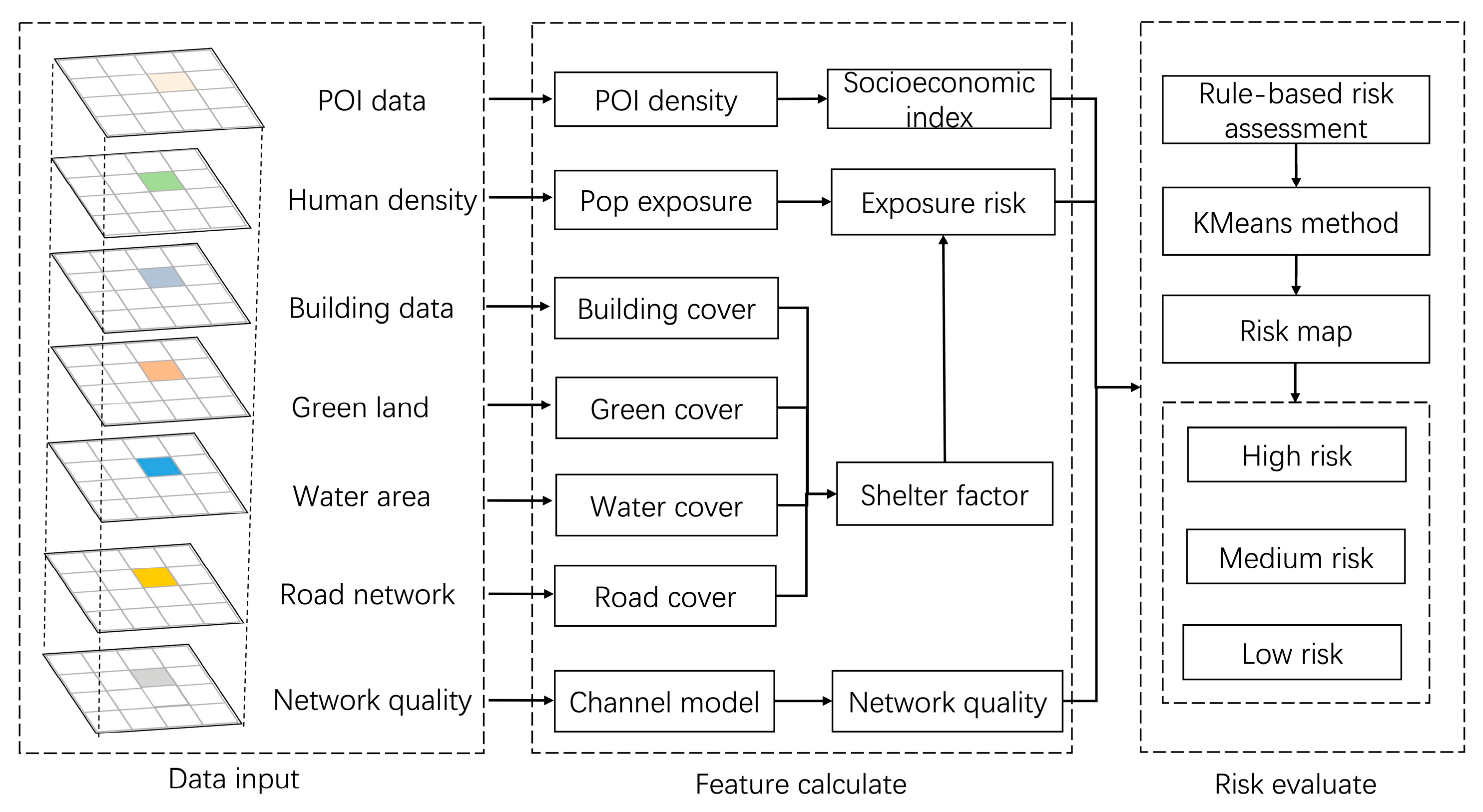
This study presents a three-dimensional low-altitude airspace risk assessment framework that integrates multi-source geospatial and communication data. As illustrated in Figure 1, the framework comprises three primary modules: data input, feature extraction, and risk evaluation. In the data input stage, multiple datasets are incorporated, including building footprints, green coverage, water bodies, population density, points of interest (POIs), road networks, and network signal strength. Collectively, these datasets characterize the physical environment, human activity intensity, and communication conditions of urban airspace. To better perform airspace calculations, we divide the study area into N*M grids of equal size. Each grid cell is assigned a unique code. All attribute information is spatially joined with the grid cells, storing the relevant attributes using the grid as the basic unit. It should be noted that Figure 1 primarily illustrates the conceptual workflow and data framework. Detailed descriptions of data sources, acquisition methods, and preprocessing procedures are provided in Section 3.1.

During feature extraction, these data are transformed into three key dimensions, which form the theoretical basis of the risk model. Section 2.1 elaborates on the construction of population exposure risk, derived from population density and multiple environmental shelter factors (including building, green, road, and water cover). This section quantifies potential human exposure under UAV failure scenarios and examines how varying land-cover characteristics modulate the degree of protection against crash impacts. Section 2.2 introduces the socioeconomic index, represented by POI density, to capture the spatial concentration of human activities and evaluate the potential socioeconomic consequences associated with UAV-related incidents. Section 2.3 describes the modeling of network quality using a statistical radio propagation framework to assess communication reliability across different altitudes. Collectively, these three components—population exposure risk, socioeconomic attributes, and network quality—form the core analytical dimensions of the proposed three-dimensional low-altitude airspace risk assessment model.

Section 2.4 presents the risk evaluation process, where the normalized indicators are integrated through a rule-based weighting scheme, followed by an unsupervised K-Means clustering procedure that classifies grid cells into high-, medium-, and low-risk categories. This multi-dimensional framework enables the model to jointly account for population, environmental, and communication factors, providing a comprehensive theoretical foundation for low-altitude UAV safety assessment.

2.1. Risk of Population Exposure

To begin, we calculate the ground collision risk associated with UAVs, defined as the likelihood of injury or fatality among ground populations resulting from a UAV crash. This risk, often referred to as incident frequency, is commonly assessed using a probabilistic risk model. According to prior research [18], the model requires population density and the computation of the exposure area for individuals affected by a UAV collision. The exposure area is determined by factors including the average radius and height of a person, the UAV’s average radius, and its glide angle. Next, the probability of injury to an individual in a collision is calculated by considering the shelter factor, the UAV’s mass, and its flight speed. If a collision occurs, the incident rate is generally assumed constant. The incident rate is generally assumed constant if a collision occurs. Finally, by multiplying the exposure area, the individual injury probability in a collision, the post-collision event probability, and the population density, we can estimate the risk of population exposure in the event of a UAV collision.

$$P_{risk}\left(i\right)=A_{exp}\times \rho \left(i\right)\times P_{single}\left(i\right)\times P_{fatality}$$

(1)

$$A_{exp}=\pi \times {(r_p+r_{UAV})}^2\times \sin \delta +2\times (r_p+r_{UAV})(h_p+h_{UAV})\times \cos \delta$$

(2)

$$\rho \left(i\right)={\displaystyle \frac{Pop\left(i\right)}{{Area}_{grid}\left(i\right)}}$$

(3)

$$P_{single}\left(i\right)={\displaystyle \frac{1-k\left(i\right)}{1-2k\left(i\right)+2\sqrt{\frac{\alpha }{\beta }{[\frac{\beta }{E}]}^{\frac{3}{P_s\left(i\right)}}}}}$$

(4)

$$k\left(i\right)=\mathrm{m}\mathrm{i}\mathrm{n}\left[{\displaystyle \frac{1}{{[\frac{\beta }{E}]}^{\frac{3}{P_s\left(i\right)}}}}\right]$$

(5)

Here, $P_{risk}\left(i\right)$ represents the risk of a drone collision with ground unit $i$. $A_{exp}$ denotes the area of exposure in the event of a collision between an individual and a drone, which depends on the average radius $r_{UAV}$ of the drone, the average radius $r_p$ of a human, the average height $h_p$ of a human, and the drone’s glide angle $\delta$. $\rho \left(i\right)$ represents the population density of ground unit $i$, determined by the number of people $Pop\left(i\right)$ and the area of the grid unit ${Area}_{grid}\left(i\right)$. $P_{single}\left(i\right)$ represents the probability of an individual being injured in a collision within unit $i$, which is related to the ground shelter factor $P_s$ and the kinetic energy generated by the drone upon landing. According to Primatesta et al. [9], the parameter $\alpha$ represents the impact energy when $P_s=6$ and $P_{single}=50\%$. And the parameter $\beta$ represents the impact energy required when $P_s$ approaches 0, meaning there is almost no ground cover, and the collision probability $P_{single}$ also approaches 0. E denotes the expected energy, expressed as $E=\left[E_{imp}\right(i\left)\right]$, where $E_{imp}\left(i\right)=m{v}^2$. Here, $E_{imp}\left(i\right)$ represents estimated kinetic energy at the impact location $i$. This value is a function of the impact velocity $v$, which may vary with the drone’s mass $m$ and its descent trajectory. Finally, $P_{fatality}$ represents the probability of casualties occurring after a ground collision and is generally considered a fixed value.

2.1.1. Shelter Factor

The shelter factor is defined as the degree to which ground objects can prevent injury to people by obstructing a falling drone. This factor depends on the type and area coverage of ground objects. Common types of ground cover include buildings, green spaces, water bodies, and roads, among others. Some research has established different shelter factors for these ground cover types [19]. However, a grid unit may contain many different types of shelter factors. The total shelter factor for ach grid unit is calculated by weighting the area of each ground cover type by its corresponding shelter factor. The total shelter factor of the grid unit is then obtained by summing the shelter factor values of all ground covers within the grid unit.

$$P_s\left(i\right)={\sum }_{j=1}^k\sum _{m=1}^n{\displaystyle \frac{{Shelter}_i\left(m\right)\times S\left(j\right)}{{Area}_{grid}\left(i\right)}}$$

(6)

Here, $P_s\left(i\right)$ represents the total shelter factor value of all obstacles in grid unit $i$, ${Area}_{grid}\left(i\right)$ is the area of grid unit $i$, ${Shelter}_i\left(m\right)$ denotes the area of the $m$-th ground cover of type $j$ within the grid unit, and $P_s\left(i\right)$ represents the shelter factor value for obstacles of type $j$, with the specific values shown in

Table 1. The shelter factor of different ground factor.

Typical Ground Cover	Shelter Factor
Agricultural land, water area, green land, etc.	0
Sparse obstacles	2.5
Low-rise building	5
High-rise building	7.5
Factories, etc.	10

.

2.1.2. Population Density

Population density is a critical indicator for determining crowd exposure risk, which can be calculated using population distribution data. Higher values indicate greater population density and a more crowded area, while lower values indicate a sparser population within the grid unit. There are various methods to obtain population distribution data, such as urban traffic data [20], mobile phone signaling data derived from individual location records [21], social media check-in data [22], and location data from map applications [23]. Mobile phone signaling data, due to its representation of a large and age-diverse population, is considered to have relatively low bias and more accurately reflects the actual population distribution in urban areas [24]. The population distribution data derived from mobile phone signaling data represents the number of people staying in a specific location over a given period. In order to ensure the accuracy of ground collision risk assessment, it is crucial to obtain population distribution data with fine spatial resolution, broad coverage, and minimal data bias.

2.2. Measures of Socio-Economic Characteristics

In addition to the impact of drone collisions on ground populations, the potential damage to ground socio-economic infrastructure is also considerable. POIs data describes the spatial location and attribute information of various geographical entities and is commonly used to reflect public perception of specific locations and their functional attributes [25,26]. POI data, with its large sample size and rich information, can provide insights into various urban activities. Typically, POI data includes multiple types such as commercial land, finance, green spaces, research institutions, and more. Initially, POI types can be reclassified according to specific scenario requirements into seven major categories: commercial and financial, public facilities, government institutions, transportation facilities, natural land, education and research, and residential land. Subsequently, the density of all POI types within each grid unit can be calculated to represent the economic development level within that unit. A higher POI density may indicate greater economic significance for the area.

$${POI}_d\left(i\right)=\sum _{m=1}^n{\displaystyle \frac{{POI}_m\left(i\right)}{{Area}_{grid}\left(i\right)}}$$

(7)

${POI}_d\left(i\right)$ represents the total density of all POIs within grid unit $i$, where ${POI}_m\left(i\right)$ denotes the number of POIs of type $m$ in unit $i$, and ${Area}_{grid}\left(i\right)$ represents the area of grid unit $i$.

2.3. Simulation of Network Quality

We propose a statistical radio frequency propagation model to estimate the network environment for drones flying at different altitudes. Evaluating network communication quality in urban airspace requires consideration of parameters associated with urban building [27,28], as buildings can significantly obstruct and interfere with wireless signals during drone flights. To address this, we introduce a method for estimating network signal quality over large areas by incorporating surface building data. To differentiate between various urban environments, two key parameters must be calculated:

(1)

Parameter ${\lambda }_i$ represents the ratio of the area of all buildings within grid unit $i$ to the total area of that grid unit.

$${\lambda }_i={\displaystyle \frac{{Building}_{area}\left(i\right)}{{Area}_{grid}\left(i\right)}}$$

(8)

(2)

Parameter ${\gamma }_i$: Assuming that building heights in the city follow a Rayleigh distribution [29], ${\gamma }_i$ is the scale parameter of the Rayleigh distribution for the buildings in grid unit $i$.

$$P\left(h\right)={\displaystyle \frac{h}{{\gamma }_i}}exp{\displaystyle \frac{-h^2}{2{\left({\gamma }_i\right)}^2}}$$

(9)

$h$ indicates the building height in grid unit.

Based on building environment data within the city, the building parameters for each grid can be determined. A higher ${\lambda }_i$ value indicates that the grid unit has a larger building footprint area, while a higher ${\gamma }_i$ value suggests that there are more high-rise buildings within the grid unit.

To estimate signal loss in various building environments, we develop a Line-of-Sight (LoS) path calculation method using the Mean Field approach, referred to as the Mean Layer Method. In the LoS scenario, there are no obstructions between the drone and the ground base station. In contrast, the Non-Line-of-Sight (NLoS) scenario involves obstructions such as buildings or trees that block direct communication between the drone and the ground base station. This method assumes that the statistical properties of buildings within a grid unit are homogeneous, and the impact of buildings at different heights on the signal is only considered at the building edges, without accounting for signal scattering and diffraction caused by building obstructions. First, the probability of obstruction for the LoS path is calculated using the Mean Layer Method:

$$P_{LoS}\left(H_0,x\right)=\prod _{m=1}^{round({\displaystyle \frac{x}{r}})}\left\{1-{\lambda }_i{F}_{h_i}({\displaystyle \frac{H_0\times x}{m\times r}})\right.\}$$

(10)

where $r$ represents the layer radius, $x$ denotes the straight-line distance between the drone and the ground base station, $H_0$ is the vertical distance between the drone and the ground, and $m$ indicates the number of layers. $F_{h_i}\left({\displaystyle \frac{H_0\times x}{m\times r}}\right)$ is the cumulative Rayleigh probability distribution function with a scale parameter of ${\gamma }_i$, indicating that the random height variable $h_i$ is less than or equal to ${\displaystyle \frac{H_0\times x}{m\times r}}$. Additionally, the $P_{LoS}\left(H_0,x\right)$ must satisfy the condition that $P_{LoS}\left(H_0,x\right)+P_{NLoS}\left(H_0,x\right)=1$.

In the LoS scenario, path loss can be modeled using the free-space propagation model [16]. In the NLoS scenario, an additional fixed loss value is incorporated into the path loss calculated for the LoS scenario. Finally, the path losses from both the LoS and NLoS scenarios are weighted and averaged to derive the final path loss distribution.

$${PL}_{LoS}=20\log \left(d_n\right)+20\log \left(f_{MHZ}\right)+20\log \left({\displaystyle \frac{4\pi }{c}}\right)+\eta$$

(11)

$${PL}_{NLoS}=20\log \left(d_n\right)+20\log \left(f_{MHZ}\right)+20\log \left({\displaystyle \frac{4\pi }{c}}\right)+\eta +10P_{LoS}\log \left(d_n\right)$$

(12)

$$\mathsf{\Lambda }=P_{LoS}\times {PL}_{LoS}+P_{NLoS}\times {PL}_{NLoS}$$

(13)

where ${PL}_{LoS}$ represents the path loss calculation in the absence of obstruction, and ${PL}_{NLoS}$ represents the path loss calculation in the presence of obstruction.$f_{MHZ}$ represents the carrier frequency, specifically the widely used 4.9 GHz band, with this study considering an operating frequency of 4850 MHz. In practice, this corresponds to the 4.9 GHz allocation of China Mobile (headquartered in Beijing, China)—covering the range 4800–4960 MHz with a total bandwidth of 160 MHz. $d_n$ represents the straight-line distance between the drone and the ground base station. $c$ represents the speed of light, and $\eta$ denotes the reference path loss.

We then assess the path loss of network signals at different heights. First, the airspace below 300 m is divided into different height levels at fixed intervals (e.g., 10 m). The airspace at various heights is partitioned using the same grid system as on the ground, with each grid being 500 m by 500 m. Next, drones are randomly sampled within the airspace at different altitudes, while base station locations are randomly sampled within non-building covered areas of the ground grid units. Considering that drones in flight are not influenced by all ground base stations, we assume that drones are primarily affected by base stations within a 500 m radius of the corresponding ground grid center. We employ a Monte Carlo simulation process to model the interaction between drones and ground base stations. By performing multiple simulation iterations, we obtain the mean and confidence interval of the signal obstruction coefficient for each grid, which is then incorporated into the channel propagation model. This allows us to calculate the network signal quality for each grid within a large-scale area.

2.4. Risk Classification Algorithm of Airspace

By integrating the calculated attribute features of each grid unit, we classify the low-altitude airspace risk. These features include population exposure probability risk based on population density and shelter factor, POI density, and network signal quality. A higher population exposure probability risk suggests a greater likelihood of ground casualties in the event of a drone crash. A higher POI density implies greater potential economic loss in the event of a collision. Similarly, higher network signal quality values correspond to better communication conditions for UAV operations.

To avoid discrepancies in classification rules caused by differences in magnitude or meaning among various features, we first normalize the different features to ensure consistency in their scales. Given that different feature indicators contribute differently to airspace risk, we assign different weights to each feature. The standardized data is then multiplied by the corresponding weights to adjust the importance of each feature in the classification process. Finally, we use the adjusted data to train a KMeans method to classify the risk levels of all grid units in the airspace into high, medium, and low levels.

3. Results

In this section, we conduct experiments to achieve three objectives: (1) Assess the various attribute factors that may affect the risk of low-altitude drone flights and potential ground collisions. (2) Evaluate the risk levels of urban airspace at different height layers. (3) Provide a visual representation of the risk levels in low-altitude airspace.

3.1. Data Description

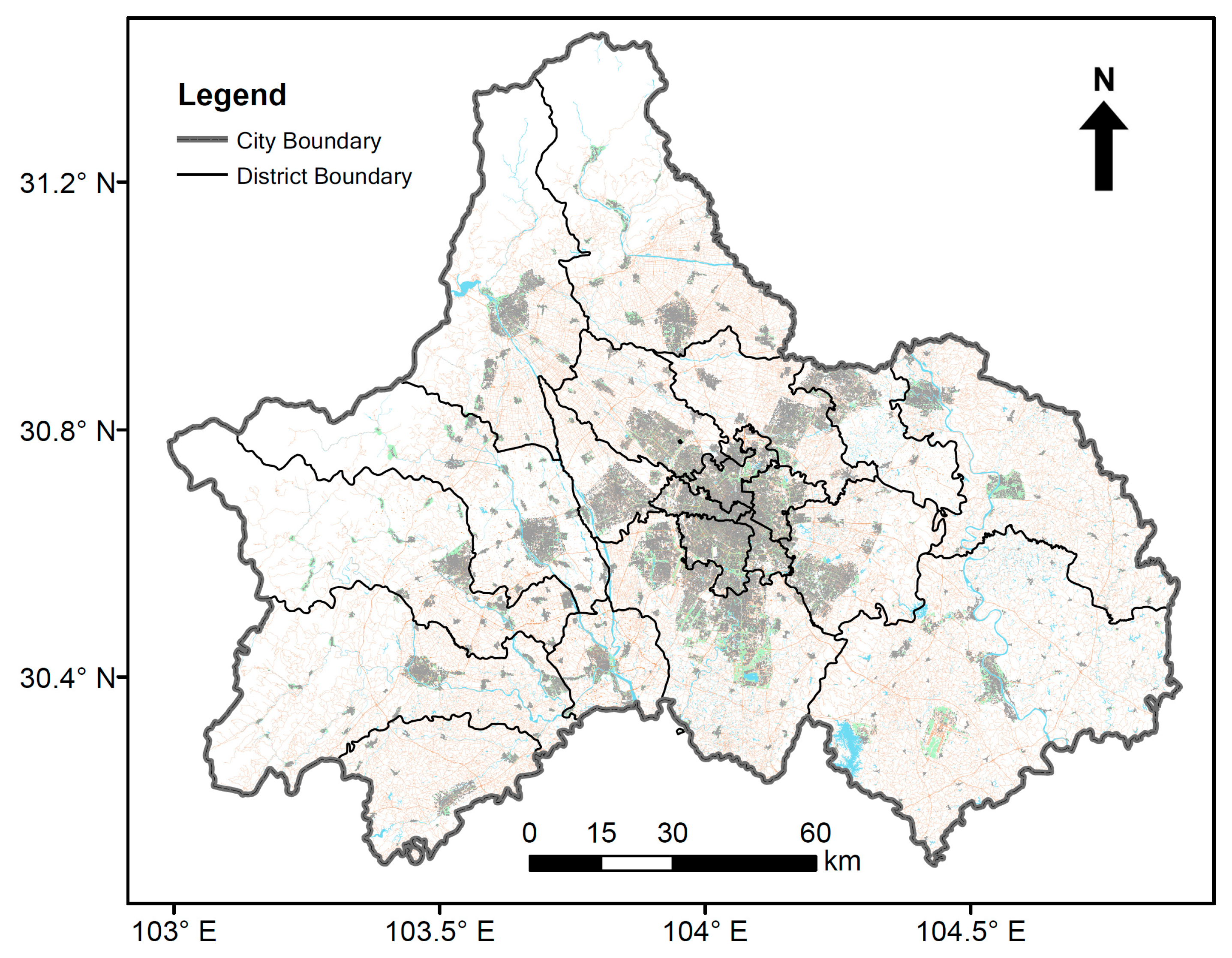
Taking Chengdu as a case study (Figure 2), we introduced various data types to conduct experiments. Chengdu is one of the largest cities in Western China, with a resident population of over 21 million. The city performs multiple functions and features a complex urban environment, including two general aviation airports: Tianfu and Shuangliu. Additionally, Chengdu has partially opened its lo-altitude airspace, reflecting a significant demand for the opening and utilization of low-altitude airspace. Therefore, Chengdu serves as an ideal subject for studying low-altitude airspace risk assessment. The entire region of Chengdu was divided into 500 m $\times$ 500 m study units, and the following categories of data were primarily collected: (1) POI data; (2) land cover data, including green space, building environment data, and so on; (3) population density data.

3.1.1. Land Cover Data

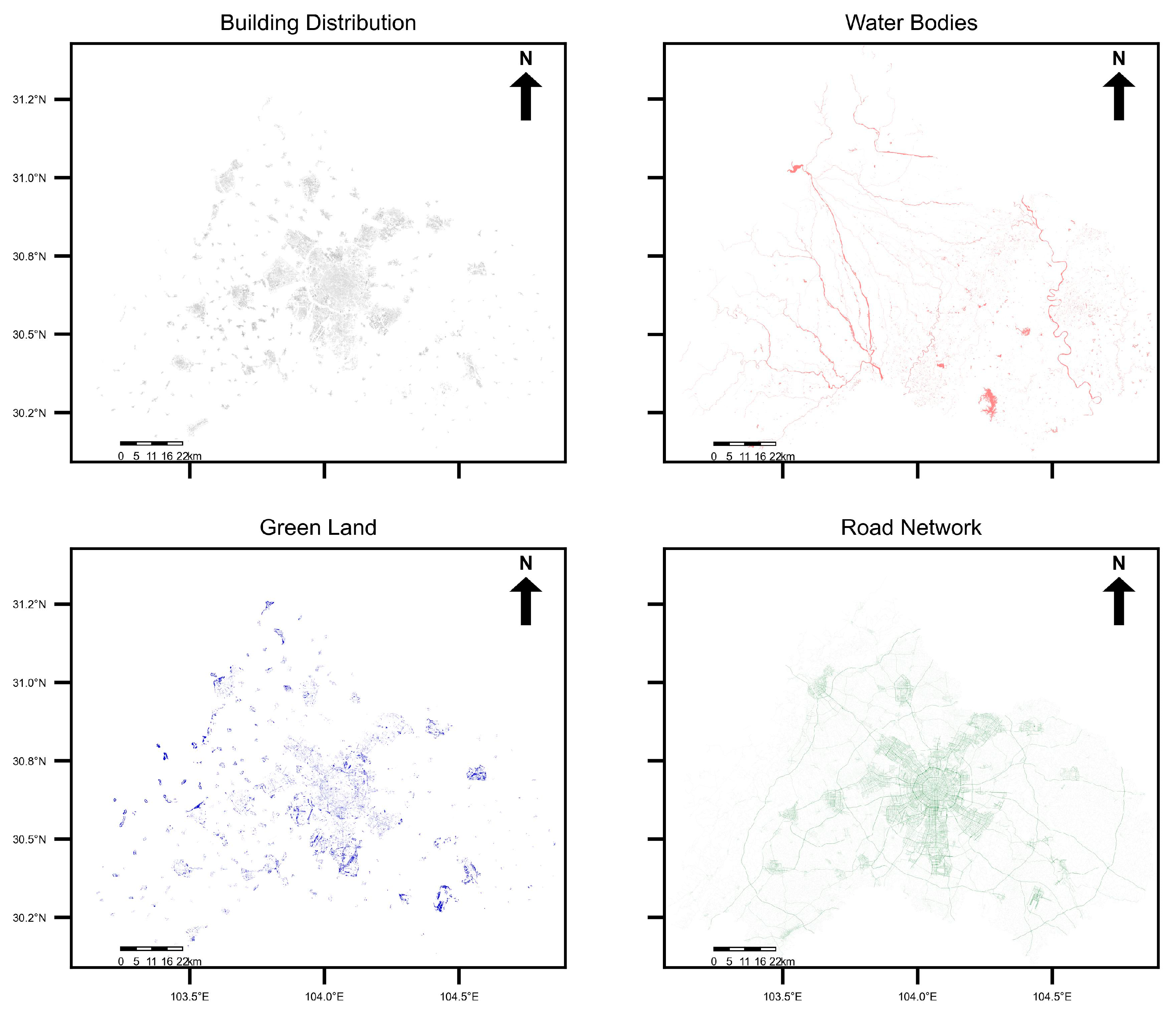
The land use data utilized in this study is derived from high-resolution 1:2000 scale map data, which includes various land use types such as green spaces, water bodies, roads, and buildings. This data allows for a more detailed representation of actual building dimensions, road widths, and other relevant information. Figure 3 presents the raw data for different land cover types. Each land cover includes attribute information such as latitude, longitude, length, and area. Building data also includes height characteristics of different buildings. By matching different land parcels with grid units, the area of each land cover within each grid unit can be calculated.

3.1.2. POIs Data

POIs serve as fundamental spatial units that reflect the functional attributes of specific area. The POI data utilized in this study was obtained from China Mobile Shanghai Industrial Research Institute, a professional mapping company, and represents data collected in 2023. The initial POI types include ten categories: general landmarks, cultural and recreational facilities, commercial institutions, scientific research and education, transportation services, tourism, shopping guides, public services, government agencies, and catering and accommodation, totaling 1,890,887 POI points. The POI data includes a wide variety of classification types, but our primary focus is on the total number of POI points within each grid unit. Therefore, we do not further classify or adjust for different POI types.

To ensure data quality and mitigate the influence of extreme values, the POI dataset underwent several preprocessing steps prior to analysis: (1) coordinate validation and reprojection to the project’s working coordinate reference system (CRS); (2) spatial filtering within the study area boundary and removal of records with missing or implausible coordinates (e.g., points located outside the study area); (3) deduplication of identical or near-identical records based on coordinate and name attributes; and (4) assignment of each POI to the grid system adopted in this study, followed by computation of total POI counts per grid cell.

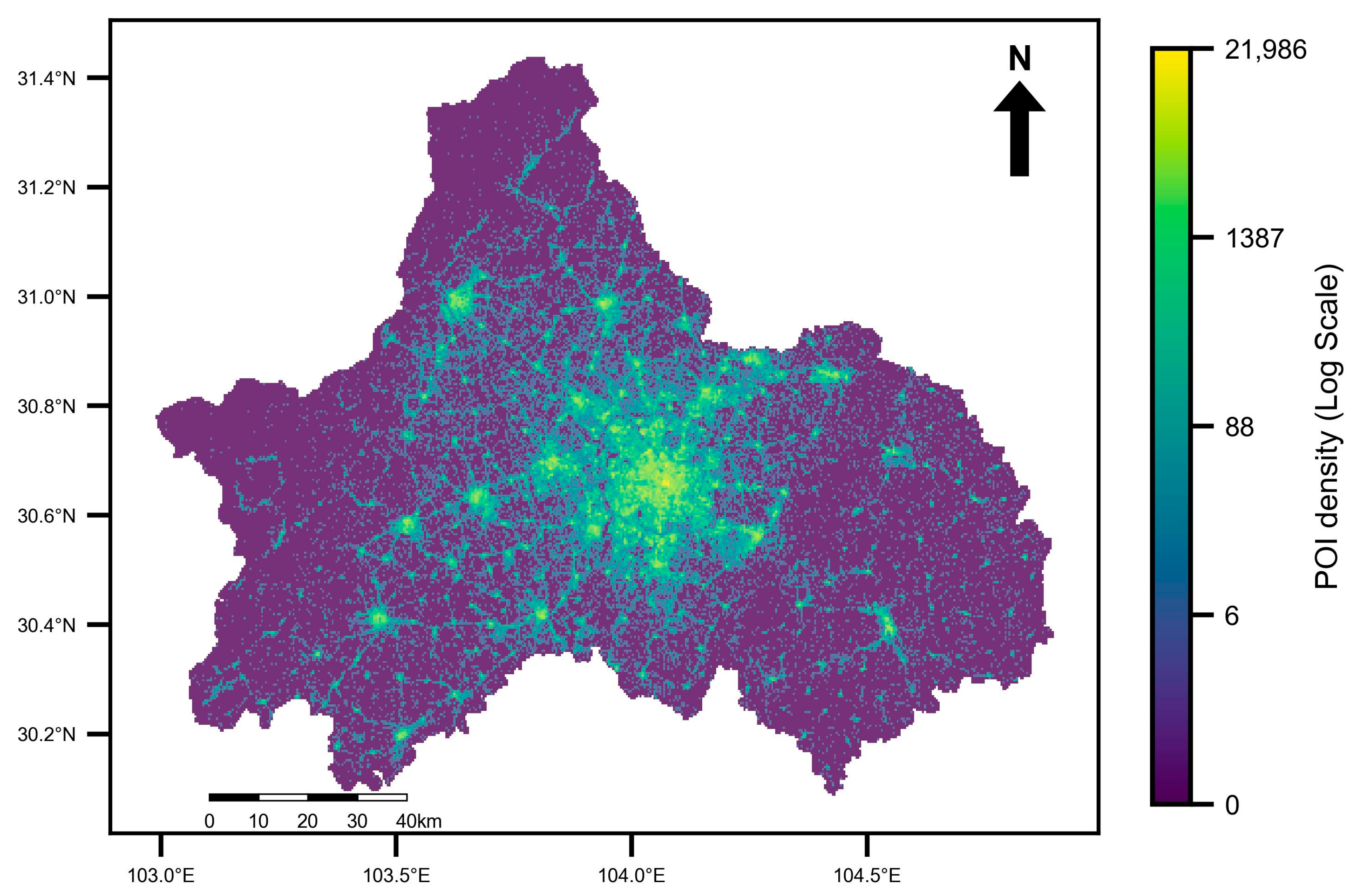
Figure 4 illustrates the spatial distribution of POIs data across the study area. The distribution exhibits pronounced clustering in the urban center and along major transportation corridors, with high-density hotspots coinciding with the central business district, major rail and metro stations, and large commercial complexes. In contrast, suburban and industrial zones show markedly lower POI densities. These spatial patterns—characterized by strong central clustering and corridor-oriented concentration—validate the use of aggregated POI counts as a proxy for functional intensity and potential human exposure within each grid cell.

3.1.3. Population Distribution Data

The population distribution data used in this study was provided by China Mobile, and was derived from mobile phone signaling data collected throughout December 2023. China Mobile aggregates anonymized location information by accessing cell tower connections from mobile devices. By recording the movements of millions of anonymous mobile users across different locations, they calculate and compile the number of visits to each location on an hourly and daily basis, thereby representing the spatial distribution of population activity.

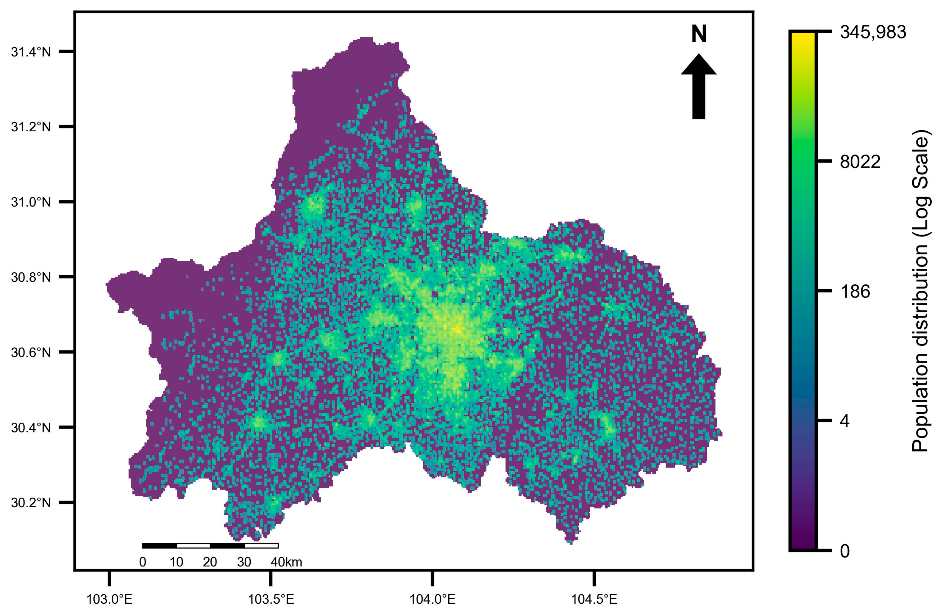
For this study, the signaling data from the entire month of December 2023 was matched to the 500 m × 500 m grid of the study area, and the average population count per grid cell over the month was used to represent the final population distribution dataset. Figure 5 illustrates the spatial distribution of the averaged population data in Chengdu, highlighting a clear pattern of higher population density in the central urban areas and lower density toward the periphery urban areas. Due to significant regional variations in the data, a logarithmic transformation was applied to the population values to enhance visualization. To prevent infinite values during the transformation, grid cells with zero population were replaced with a very small constant prior to the logarithmic operation.

3.2. The Result of Population Exposure Risk

To assess the risk of population exposure resulting from a drone crash, we initially calculated the total shelter factor of all land cover types within each region. Using the area of different land covers within the grid cells and their corresponding sheltering factors, we calculated the shelter factors for each land cover type within the grid cells. The total shelter factor for each grid cell was then obtained by summing the shelter factors of all land covers. Specifically, for buildings, the shelter factor varies with height. Therefore, we first categorize buildings as either high-rise or low-rise. Residential buildings with a height greater than 27 m and other non-single-story civilian buildings with a height greater than 24 m are classified as high-rise. All other buildings are considered low-rise.

Figure 6 illustrates the shelter factor values of various land cover types within each grid cell, excluding green spaces and water bodies due to their sheltering factor being zero. The sheltering factors across different types generally exhibit a pattern of higher values in the central urban areas and lower values in the peripheral regions. However, certain peripheral areas exhibit high shelter factors, indicating regions with relatively dense coverage. This pattern aligns with typical urban trends, where city centers are densely populated with buildings, including many high-rise structures, while peripheral regions are less densely developed and predominantly feature low-rise buildings. The presence of satellite towns in peripheral regions can, however, result in areas with dense building coverage or a significant number of high-rise buildings.

In conjunction with the population density of each region and the relevant parameters of both drones and humans (as shown in

Table 2. The relevant parameter of risk exposure model.

Field	Description	Value
$r_p$	Average radius of a person	0.2 m
$h_p$	Average height of a person	2 m
$r_{UAV}$	Average radius of a drone	0.35 m
$\delta$	Glide angle of the drone	${45}^{°}$
m	Weight of the drone	1.5 kg
v	Average flight speed	10 m/s

), we calculated the risk values for population exposure in different areas. It is important to note that the selection of parameters primarily aligns with those used by Primatesta et al. [9]. For this study, we assumed fixed values for the average radius of a person, the average height of a person, the average radius of a drone, the drone’s glide angle, the drone’s weight, and its average flight speed. Additionally, we did not differentiate between different types of drones or descent modes (e.g., ballistic descent, parachute descent, or uncontrolled glide). This approach is justified by the primary objective of this paper, which is to assess low-altitude airspace risk in urban areas and categorize these areas into different risk levels for comparison in the event of a drone collision. This method is applicable to any type of drone and mode of descent.

The population exposure risk values indicate the potential number of injuries or fatalities in a given area resulting from a drone collision. We observed significant variations in risk values across different regions (Figure 7). In most regions, the population exposure risk is relatively low, with only a few regions exhibiting risk values exceeding 100. However, in Chengdu, a densely populated city with high population mobility, certain areas exhibit risk values greater than 1000, indicating an extremely high risk for drone operations in these zones. Additionally, the population exposure risk displays a clear spatial variation, with high-risk areas concentrated in the central urban districts. There are also some relatively high-risk regions on the outskirts. Notably, even neighboring areas can exhibit significant differences in risk values, underscoring the importance of conducting detailed risk assessments for low-altitude airspace.

3.3. The Indicator of Socio-Economic Characteristics

Many studies have shown that POI density is a significant indicator of local socioeconomic activity and is correlated with both the frequency and severity of traffic collisions. For instance, Chen et al. [30] employed an XGBoost model integrated with POI data to analyze the determinants of crash severity in autonomous vehicle operations, revealing that land use diversity and POI density were key contributors to serious traffic accidents. Similarly, Jia et al. [31] investigated the relationship between POI distributions and traffic incidents, demonstrating that areas with higher POI densities—particularly those surrounding public service facilities and medical institutions—tend to experience elevated accident rates.

In this study, we compute the overall POI density without distinguishing between specific POI categories or their relative proportions. This approach is adopted because, to the best of our knowledge, no existing research has yet established a definitive correlation between particular POI types and airspace collision risk for UAVs. Nonetheless, within grid cells of equal size, a higher total number of POIs generally reflects greater functional intensity, typically associated with higher population concentration and more diverse human activities [32]. These characteristics, as demonstrated in ground-traffic studies, correspond to a heightened likelihood of collisions and more severe consequences.

Accordingly, we employ POI density as a practical and interpretable indicator representing both local socioeconomic development and exposure risk. As illustrated in Figure 8, POI density is highest within the central urban center, while several peripheral zones also exhibit comparatively elevated densities, similar to those observed in central areas. This pattern suggests the presence of emerging urban sub-centers, where a wide range of social and economic activities are concentrated—potentially increasing exposure and risk in the event of an aerial or ground collision.

3.4. The Simulated Results of Network Signal Loss

The airspace below 300 m was divided into different height levels at 30 m intervals, and network signal losses were simulated across ten height levels.

Table 3. Statistical summary of simulated network signal losses at different heights.

Height	Minimum Signal Loss (dB)	Maximum Signal Loss (dB)	Mean Signal Loss (dB)	Standard Deviation (dB)
30	−44.07	−40.38	−43.79	0.77
60	−38.05	−33.60	−37.58	1.19
90	−34.53	−29.64	−34.01	1.31
120	−32.03	−26.83	−31.43	1.48
150	−30.09	−24.65	−29.47	1.55
180	−28.51	−22.87	−27.86	1.60
210	−27.17	−21.36	−26.52	1.61
240	−26.01	−20.06	−25.34	1.65
270	−24.99	−18.91	−24.33	1.63
300	−24.07	−17.88	−23.40	1.66

presents the statistical results of simulated network signal losses at various heights. Less negative signal loss values indicate better network signal quality. As the height increases, the network signal loss improves, ranging from −44.07 dB at lower heights to −17.88 dB at higher heights, with the mean signal loss increasing from −43.79 dB at 30 m to −23.4 dB at 300 m. Notably, at heights of 150 m or below, significant signal loss occurs due to building obstruction, with signal losses varying between −44.07 dB and −24.65 dB, and substantial differences between various height levels. At heights of 180 m and above, network signal losses range from −28.51 dB to −17.88 dB. It is evident that as height increases, the difference in network signal losses across height levels diminishes. This is because fewer buildings obstruct the signal at higher elevations, particularly since the number of buildings exceeding 180 m in Chengdu is relatively low, reducing the obstruction effects on unmanned aerial vehicles.

We then displayed the 3D spatial distribution of simulated network signal characteristics at various heights. For clarity, Figure 9a,b present the simulated network signal estimates for six specific heights: 30 m, 90 m, 150 m, 180 m, 240 m, and 300 m. The spatial maps reveal that as height increases, network signal quality improves, though the overall spatial trend remains consistent. All layers show a pattern where the signal strength is relatively higher in the most urban areas and poorer in the peripheral regions. To further observe the local characteristics of each layer, we present the 2D network signal quality distribution maps for the 30 m and 300 m height airspace in Figure 10. The results indicate that the spatial distribution of network signal quality at 30 m differs from that at 300 m, though both generally exhibit lower signal quality in the city’s central area, with relatively higher signal quality in surrounding areas. At 30 m, the network signal quality is uniformly low across the entire core area, with higher quality in the surrounding regions. This is likely due to the high density of buildings taller than 30 m within the core area, leading to significant signal attenuation caused by building obstructions. At 300 m, the network signal quality distribution shows lower signal quality in the center of the core area, while nearby regions have higher signal quality. This could be because the central area contains many super-tall buildings, whereas other areas have fewer such structures. When the UAV reaches a height of 300 m, most buildings no longer significantly interfere with airborne network signals. The overall pattern of network signal distribution at other heights is similar, but each height exhibits certain spatial differences. Therefore, it is essential to conduct simulation assessments of network signal quality at different heights.

3.5. Risk Map of Low-Altitude Airspace at Different Heights

Based on various datasets, we extracted population exposure risk, socioeconomic attributes, and network signal loss across different heights. To ensure the robustness of the proposed risk model, potential redundancy among these indicators was examined using variance inflation factor (VIF) analysis (see

Table 4. Results of the collinearity test.

Feature	VIF
Population density	2.09
Build cover	2.01
Green cover	1.19
Road cover	2.36
Water cover	1.08
POI density	2.16
Path loss	1.38

). All VIF values were below 5, indicating no significant multicollinearity and confirming that each indicator provides distinct and meaningful information. In addition, the indicators differ in both magnitude and significance. Prior to risk classification, all indicators were normalized to eliminate scale effects. On this basis, a sensitivity analysis was conducted to evaluate the relative contribution of each indicator to the overall risk classification. The results revealed that population exposure risk and network quality exerted the strongest influence on model outcomes, whereas socioeconomic factors primarily modulated local spatial variations in risk. These findings confirm that the three dimensions—population exposure, socioeconomic attributes, and network quality—provide complementary and non-redundant information essential for comprehensive low-altitude airspace risk assessment.

Accordingly, weights of [1, 0.5, 0.6] were assigned to population exposure risk, socioeconomic attributes, and network signal loss, respectively. The weighting scheme was determined based on both evidence from existing literature and results of model sensitivity tests. Previous studies [12] have demonstrated that population exposure is the most direct determinant of UAV-related risk, as it quantifies potential human casualties. In contrast, socioeconomic and communication-related factors mainly influence the secondary impacts and operational reliability of UAVs.

Based on the attributes, regions were categorized into low-, medium-, and high-risk groups. To determine the optimal number of clusters, we tested multiple k values (ranging from 2 to 6) using the Elbow method and the Silhouette Coefficient. The Elbow curve exhibited a clear inflection at k = 3, indicating an appropriate balance between model compactness and interpretability. Similarly, the average Silhouette score reached its local maximum at k = 3, suggesting that this configuration yields the most distinct and well-separated grouping of risk features. From an operational perspective, the three-cluster configuration corresponds to the commonly adopted low-, medium-, and high-risk classification in UAV airspace safety assessments [33]. Therefore, k = 3 was selected as a statistically robust and practically meaningful choice.

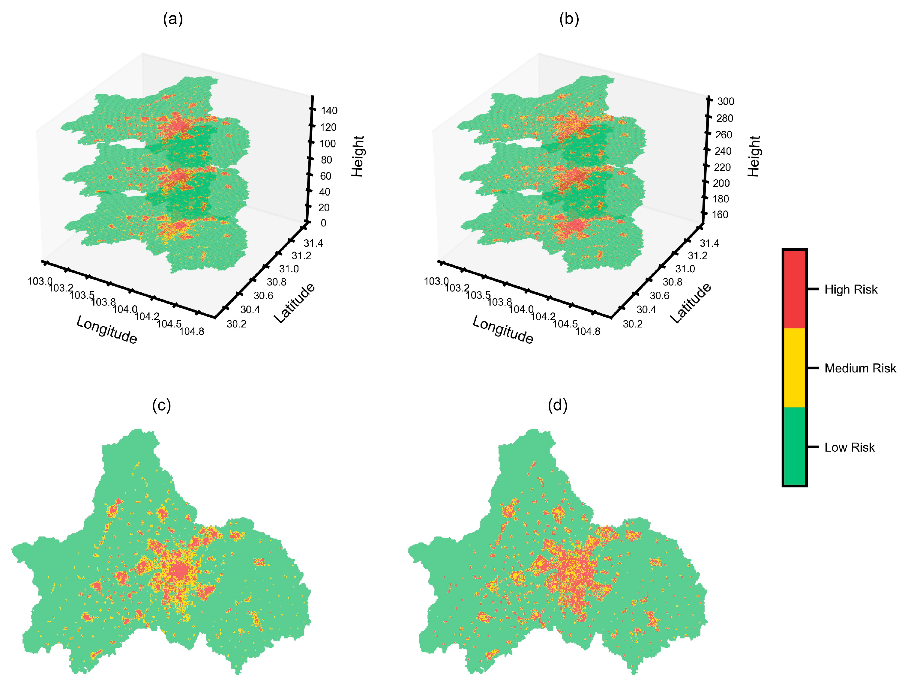
Figure 11 illustrates the 2D and 3D spatial representations of airspace risk at different heights. The 3D airspace risk map shows the risk categories at heights of 30 m, 90 m, 150 m, 180 m, 240 m, and 300 m. Across all layers, the majority of the urban area falls within the low-risk category, accounting for approximately 84–87% of the city. High-risk regions are concentrated in the central urban core, with medium-risk areas typically surrounding these zones, while peripheral areas remain predominantly low-risk. This three-dimensional representation of airspace at different heights facilitates comparison of risks at varying heights and further demonstrates that the risk levels associated with UAVs can differ at the same 2D location depending on the height. Previous airspace risk studies have predominantly focused on a 2D perspective, which can lead to inaccuracies in risk assessment.

Although the overall spatial patterns are similar, significant differences exist in both the magnitude and spatial distribution of risk levels across different altitude layers. To better visualize local variations, Figure 11c,d illustrate the risk maps for airspace at heights of 30 m and 300 m, respectively. At 30 m, the airspace risk levels show a progressive trend. The central urban area displays higher risk values, predominantly classified as high-risk regions, surrounded by medium-risk regions. The peripheral regions, further from the central city, are generally low-risk regions, though some areas, often at the center of these regions, exhibit higher risk levels. At 300 m, the risk distribution becomes more heterogeneous. In the city center, high- and medium-risk zones are interspersed, suggesting a partial reduction in risk compared to lower altitudes, while some peripheral zones exhibit increased risk levels. Notably, the proportion of high-risk zones rises from 5.9% at 30 m to 9.1% at 300 m. This phenomenon can be attributed to the changing interaction between altitude and potential impact severity: although the probability of UAV–ground interactions may decrease with altitude, the potential consequences of a fall increase due to greater kinetic energy, thereby raising the overall assessed risk.

Expanding the airspace risk assessment from two to three dimensions allows for the observation of airspace risk changes at both global and local levels. Comparative analysis of airspace risk across different altitude layers reveals significant local variations in risk values at different heights. Consequently, a three-dimensional airspace risk assessment provides a more accurate representation of risk, enhancing safety assurance for UAV operations at varying heights.

4. Discussion

4.1. The Sensitivity Analysis of Airspace Risk

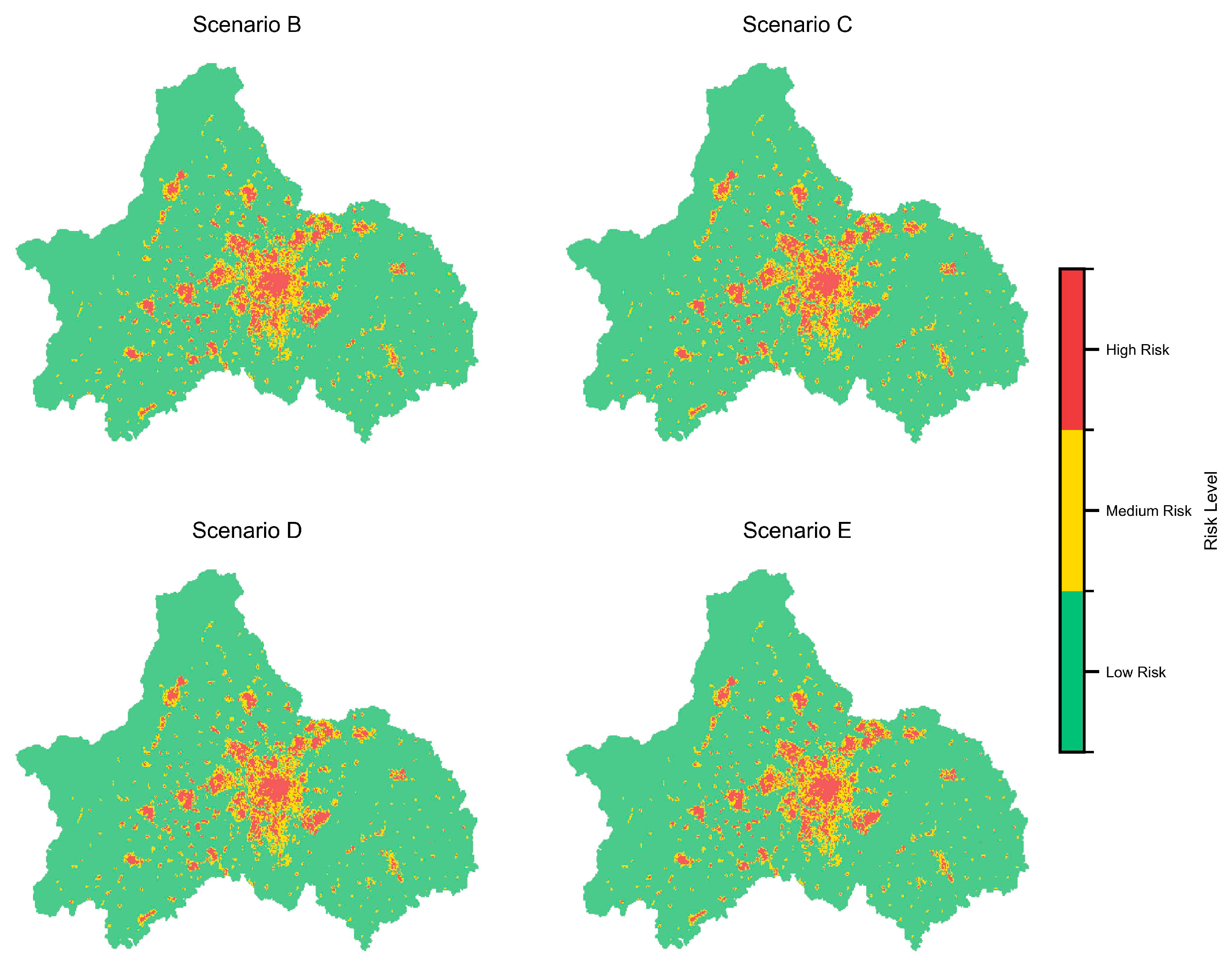
To evaluate the stability of the weighting scheme [1, 0.5, 0.6], which was assigned to population exposure risk, socioeconomic attributes, and network signal loss, a perturbation-based sensitivity analysis was conducted. In this analysis, each indicator’s weight was varied by ±20% while maintaining the total normalized weight at 1. Five alternative weighting scenarios (A–E) were designed, as presented in

Table 5. The perturbation-based sensitivity analysis of weighting scenario.

Scenario	Population Exposure	Socioeconomic	Network Signal	Normalized Weights
A (Baseline)	1.0	0.5	0.6	[0.48, 0.24, 0.28]
B (+20% Population)	1.2	0.5	0.6	[0.52, 0.22, 0.25]
C (−20% Population)	0.8	0.5	0.6	[0.42, 0.26, 0.32]
D (+20% Socioeconomic)	1.0	0.6	0.6	[0.46, 0.27, 0.27]
E (+20% Network quality)	1.0	0.5	0.8	[0.43, 0.22, 0.35]

. For each scenario, the composite risk feature was recalculated and reclassified into low-, medium-, and high-risk levels using the same quantile thresholds. The results indicate that the spatial agreement among all scenarios remained consistent (see Figure 12), with the proportion of different risk areas varying by less than 5% across all cases. These findings demonstrate that moderate variations in the indicator weights exert minimal influence on the spatial distribution of risk classification, confirming that the adopted weighting scheme ([1, 0.5, 0.6]) is both theoretically sound and empirically robust.

4.2. Comparative Analysis with Other Risk Literature

Compared with existing studies, such as Primatesta et al. (2019, 2020) [18,19] and Milano et al. (2022) [14], which primarily focus on two-dimensional ground risk mapping, the proposed framework builds upon and extends the established probabilistic risk assessment paradigm. Previous research consistently demonstrates that high-risk areas generally coincide with densely populated regions and locations with limited environmental shielding, whereas low-risk areas correspond to less populated or well-protected zones. Our approach reproduces these classical patterns, validating the robustness of the model. Moreover, by integrating multi-source data—including population density, points of interest, and environmental features—our method enhances the spatial characterization of risk, providing a richer and more comprehensive representation of urban airspace hazards than conventional 2D maps. This integration demonstrates that the proposed framework not only preserves the theoretical foundations of earlier studies but also advances them by systematically incorporating multiple data layers into a three-dimensional assessment.

By comparing risk maps across different altitude layers, we further illustrate how spatial risk patterns vary with height. While overall trends remain broadly consistent, notable differences emerge in both the magnitude and spatial distribution of risk at each layer. This vertical differentiation indicates that traditional 2D risk maps cannot fully capture the multi-layered complexity of urban airspace. The three-dimensional framework thus aligns with established theoretical foundations while providing new insights into altitude-dependent risk evolution. These findings underscore the importance of considering vertical stratification in UAV safety management and offer practical guidance for future multi-layered airspace planning and risk mitigation strategies.

5. Conclusions

Expanding the airspace risk assessment from a two-dimensional to a three-dimensional analysis enables a more comprehensive evaluation of risks across varying heights, thereby effectively enhancing the safety of low-altitude UAV flights and providing a foundation for route planning. Based on this, this paper integrates multiple influencing factors to propose a three-dimensional low-altitude airspace risk assessment method. First, the ground collision risks, which estimate potential fatalities or injuries from UAV crashes, are calculated based on factors such as population density and shelter factors. Additionally, POI density is computed for each region as a socioeconomic indicator to evaluate the impact of UAV crashes on ground socioeconomic infrastructure. Second, a network evaluation model is constructed to assess the quality of network signal losses at different heights across a large-scale airspace. Finally, the ground collision risks, socioeconomic characteristics, and network signal quality for each region are combined and classified into low, medium, and high-risk levels using machine learning algorithms, resulting in a three-dimensional airspace risk map.

The three-dimensional airspace risk map reveals that while the overall risk distribution trend is similar across different height layers, there are significant local variations. The airspace risk generally shows a pattern of high and medium risks interspersed in central urban areas, with low-risk regions predominantly found in peripheral areas, though some medium-to-high-risk regions are also present. Notably, we find that the airspace risk for the same grid unit varies across different heights, further underscoring the necessity of evaluating three-dimensional airspace risks.

Despite the innovative three-dimensional airspace risk assessment method proposed in this study, several limitations remain. First, the method is designed for large-scale airspace, which may reduce the accuracy of local airspace risk assessments. This is because airspace risk is influenced not only by factors considered in this study, such as population density, obstructions, socioeconomic factors, and network signal quality, but also by additional elements like low-altitude airspace usage and the electromagnetic environment. Second, in simulating network signal quality at different altitude layers, we simplified the model by considering only LOS and NLOS scenarios, thereby neglecting the more complex signal obstructions caused by reflections and diffraction between the UAV and ground-based stations [34]. Given the numerous and complex factors influencing airspace risk, this study focuses on proposing a three-dimensional risk assessment method that integrates multi-source data. Future research will aim to incorporate more variables affecting airspace risk dynamics to improve the accuracy of risk assessments and ensure the safe operation of UAVs in low-altitude environments.

References

1. Fan, B.K.; Li, Y.; Zhang, R.Y. Initial Analysis of Low-Altitude Internet of Intelligences (IOI) and the Applications of Unmanned Aerial Vehicle Industry. Prog. Geogr. 2021, 40, 1441–1450. [Google Scholar] [CrossRef]
2. Xu, C.; Liao, X.; Tan, J.; Ye, H.; Lu, H. Recent Research Progress of Unmanned Aerial Vehicle Regulation Policies and Technologies in Urban Low Altitude. IEEE Access 2020, 8, 74175–74194. [Google Scholar] [CrossRef]
3. Dalamagkidis, K.; Valavanis, K.P.; Piegl, L.A. On Integrating Unmanned Aircraft Systems into the National Airspace System: Issues, Challenges, Operational Restrictions, Certification, and Recommendations; Springer: Dordrecht, The Netherlands, 2012; ISBN 978-94-007-2478-5. [Google Scholar]
4. Clothier, R.; Walker, R.; Fulton, N.; Campbell, D. A Casualty Risk Analysis for Unmanned Aerial System (UAS) Operations over Inhabited Areas. In Proceedings of the AIAC12: 2nd Australasian Unmanned Air Vehicles Conference, Bristol UAV Conference, Melbourne, Australia, 19–22 March 2007; pp. 1–16, ISBN 978-0-9803215-0-0. [Google Scholar]
5. EASA JARUS. Guidelines on Specific Operations Risk Assessment (SORA). Available online: http://jarus-rpas.org/wp-content/uploads/2023/07/jar_doc_06_jjarus_sora_executive_summary.pdf (accessed on 1 August 2025).
6. EASA. Specific Operations Risk Assessment (SORA). Available online: https://www.easa.europa.eu/en/domains/drones-air-mobility/operating-drone/specific-category-civil-drones/specific-operations-risk-assessment-sora (accessed on 1 August 2025).
7. Dalamagkidis, K.; Valavanis, K.P.; Piegl, L.A. Evaluating the Risk of Unmanned Aircraft Ground Impacts. In Proceedings of the 2008 16th Mediterranean Conference on Control and Automation, Ajaccio, France, 25–27 June 2008; pp. 709–716. [Google Scholar]
8. Lum, C.; Waggoner, B. A Risk Based Paradigm and Model for Unmanned Aerial Systems in the National Airspace. In Proceedings of the Infotech@Aerospace 2011, Infotech@Aerospace Conferences, Seattle, WA, USA, 29–31 March 2011; American Institute of Aeronautics and Astronautics: Reston, VA, USA, 2011. [Google Scholar]
9. Primatesta, S.; Cuomo, L.S.; Guglieri, G.; Rizzo, A. An Innovative Algorithm to Estimate Risk Optimum Path for Unmanned Aerial Vehicles in Urban Environments. Transp. Res. Procedia 2018, 35, 44–53. [Google Scholar] [CrossRef]
10. Primatesta, S.; Scanavino, M.; Guglieri, G.; Rizzo, A. A Risk-Based Path Planning Strategy to Compute Optimum Risk Path for Unmanned Aircraft Systems over Populated Areas. In Proceedings of the 2020 International Conference on Unmanned Aircraft Systems (ICUAS), Athens, Greece, 1–4 September 2020; IEEE: Piscataway, NJ, USA, 2020; pp. 641–650. [Google Scholar]
11. Ancel, E.; Capristan, F.M.; Foster, J.V.; Condotta, R.C. Real-Time Risk Assessment Framework for Unmanned Aircraft System (UAS) Traffic Management (UTM). In Proceedings of the 17th AIAA Aviation Technology, Integration, and Operations Conference, Denver, CO, USA, 5–9 June 2017; American Institute of Aeronautics and Astronautics: Reston, VA, USA, 2017. [Google Scholar]
12. Jiao, Q.; Liu, Y.; Zheng, Z.; Sun, L.; Bai, Y.; Zhang, Z.; Sun, L.; Ren, G.; Zhou, G.; Chen, X.; et al. Ground Risk Assessment for Unmanned Aircraft Systems Based on Dynamic Model. Drones 2022, 6, 324. [Google Scholar] [CrossRef]
13. Xu, C.; Liao, X.; Ye, H.; Yue, H. Iterative Construction of Low-Altitude UAV Air Route Network in Urban Areas: Case Planning and Assessment. J. Geogr. Sci. 2020, 30, 1534–1552. [Google Scholar] [CrossRef]
14. Milano, M.; Primatesta, S.; Guglieri, G. Air Risk Maps for Unmanned Aircraft in Urban Environments. In Proceedings of the 2022 International Conference on Unmanned Aircraft Systems (ICUAS), Dubrovnik, Croatia, 21–24 June 2022; IEEE: Piscataway, NJ, USA; pp. 1073–1082. [Google Scholar]
15. Lyu, J.; Zhang, R. Network-Connected UAV: 3-D System Modeling and Coverage Performance Analysis. IEEE Internet Things J. 2019, 6, 7048–7060. [Google Scholar] [CrossRef]
16. Al-Hourani, A.; Kandeepan, S.; Lardner, S. Optimal LAP Altitude for Maximum Coverage. IEEE Wirel. Commun. Lett. 2014, 3, 569–572. [Google Scholar] [CrossRef]
17. Al-Hourani, A. On the Probability of Line-of-Sight in Urban Environments. IEEE Wirel. Commun. Lett. 2020, 9, 1178–1181. [Google Scholar] [CrossRef]
18. Primatesta, S.; Guglieri, G.; Rizzo, A. A Risk-Aware Path Planning Strategy for UAVs in Urban Environments. J. Intell. Robot. Syst. 2019, 95, 629–643. [Google Scholar] [CrossRef]
19. Primatesta, S.; Rizzo, A.; La Cour-Harbo, A. Ground Risk Map for Unmanned Aircraft in Urban Environments. J. Intell. Robot. Syst. 2020, 97, 489–509. [Google Scholar] [CrossRef]
20. Huang, Z.; Ling, X.; Wang, P.; Zhang, F.; Mao, Y.; Lin, T.; Wang, F.-Y. Modeling Real-Time Human Mobility Based on Mobile Phone and Transportation Data Fusion. Transp. Res. Part C Emerg. Technol. 2018, 96, 251–269. [Google Scholar] [CrossRef]
21. Zhao, K.; Tarkoma, S.; Liu, S.; Vo, H. Urban Human Mobility Data Mining: An Overview. In Proceedings of the 2016 IEEE International Conference on Big Data (Big Data), Washington, DC, USA, 5–8 December 2016; IEEE: Piscataway, NJ, USA, 2016; pp. 1911–1920. [Google Scholar]
22. Liu, Y.; Sui, Z.; Kang, C.; Gao, Y. Uncovering Patterns of Inter-Urban Trip and Spatial Interaction from Social Media Check-In Data. PLoS ONE 2014, 9, e86026. [Google Scholar] [CrossRef]
23. Bao, W.; Gong, A.; Zhang, T.; Zhao, Y.; Li, B.; Chen, S. Mapping Population Distribution with High Spatiotemporal Resolution in Beijing Using Baidu Heat Map Data. Remote Sens. 2023, 15, 458. [Google Scholar] [CrossRef]
24. Chin, K.; Huang, H.; Horn, C.; Kasanicky, I.; Weibel, R. Inferring Fine-Grained Transport Modes from Mobile Phone Cellular Signaling Data. Comput. Environ. Urban Syst. 2019, 77, 101348. [Google Scholar] [CrossRef]
25. Huang, Z.; Qi, H.; Kang, C.; Su, Y.; Liu, Y. An Ensemble Learning Approach for Urban Land Use Mapping Based on Remote Sensing Imagery and Social Sensing Data. Remote Sens. 2020, 12, 3254. [Google Scholar] [CrossRef]
26. Yue, Y.; Zhuang, Y.; Yeh, A.G.O.; Xie, J.-Y.; Ma, C.-L.; Li, Q.-Q. Measurements of POI-Based Mixed Use and Their Relationships with Neighbourhood Vibrancy. Int. J. Geogr. Inf. Sci. 2017, 31, 658–675. [Google Scholar] [CrossRef]
27. Al-Hourani, A.; Chandrasekharan, S.; Kandeepan, S. Path Loss Study for Millimeter Wave Device-to-Device Communications in Urban Environment. In Proceedings of the 2014 IEEE International Conference on Communications Workshops (ICC), Sydney, NSW, Australia, 10–14 June 2014; IEEE: Piscataway, NJ, USA, 2014; pp. 102–107. [Google Scholar]
28. Xia, H.H. A Simplified Analytical Model for Predicting Path Loss in Urban and Suburban Environments. IEEE Trans. Veh. Technol. 1997, 46, 1040–1046. [Google Scholar] [CrossRef]
29. Al-Hourani, A.; Guvenc, I. On Modeling Satellite-to-Ground Path-Loss in Urban Environments. IEEE Commun. Lett. 2021, 25, 696–700. [Google Scholar] [CrossRef]
30. Chen, H.; Chen, H.; Liu, Z.; Sun, X.; Zhou, R. Analysis of Factors Affecting the Severity of Automated Vehicle Crashes Using XGBoost Model Combining POI Data. J. Adv. Transp. 2020, 2020, 8881545. [Google Scholar] [CrossRef]
31. Jia, R.; Khadka, A.; Kim, I. Traffic Crash Analysis with Point-of-Interest Spatial Clustering. Accid. Anal. Prev. 2018, 121, 223–230. [Google Scholar] [CrossRef] [PubMed]
32. Li, Z.; Jiao, L.; Zhang, B.; Xu, G.; Liu, J. Understanding the Pattern and Mechanism of Spatial Concentration of Urban Land Use, Population and Economic Activities: A Case Study in Wuhan, China. Geo-Spat. Inf. Sci. 2021, 24, 678–694. [Google Scholar] [CrossRef]
33. Air Traffic OrganizationSafety and Technical Training the Safety Management System (SMS) Manual Version 4.0. Available online: https://www.faa.gov/air_traffic/publications/media/faa_ato_SMS_manual_v4_20140901.pdf (accessed on 12 March 2024).
34. Al-Hourani, A.; Kandeepan, S.; Jamalipour, A. Modeling Air-to-Ground Path Loss for Low Altitude Platforms in Urban Environments. In Proceedings of the 2014 IEEE Global Communications Conference, Austin, TX, USA, 8–12 December 2014; IEEE: Piscataway, NJ, USA, 2014; pp. 2898–2904. [Google Scholar]
Figure 1. The framework of airspace risk assessment model.
Ijgi 14 00413 g001
Figure 2. Overview map of the study area in Chengdu.
Ijgi 14 00413 g002
Figure 3. The map of different land cover data of Chengdu city.
Ijgi 14 00413 g003
Figure 4. The spatial distribution of POIs data in Chengdu.
Ijgi 14 00413 g004
Figure 5. The population distribution of Chengdu.
Ijgi 14 00413 g005
Figure 6. The distribution of shelter factor of different land cover.
Ijgi 14 00413 g006
Figure 7. The distribution of population exposure risk in Chengdu. The Eagle Eye map illustrates the population exposure risk values for the selected central region of Chengdu.
Ijgi 14 00413 g007
Figure 8. The distribution of POI density.
Ijgi 14 00413 g008
Figure 9. The 3D map of simulated network signal loss at different heights. (a) shows the simulated 3d network signal loss map at heights of 30 m, 90 m, and 150 m. (b) shows the simulated 3d network signal loss map at heights of 180 m, 240 m, and 300 m.
Ijgi 14 00413 g009
Figure 10. The 2D map of simulated network signal loss for the 30 m and 300 m height airspace.
Ijgi 14 00413 g010
Figure 11. Risk map of low-altitude airspace at different heights. (a) 3D airspace risk maps at heights of 30 m, 90 m, and 150 m. (b) 3D airspace risk maps at heights of 180 m, 240 m, and 300 m. (c) 2D risk map for the 30 m height airspace. (d) 2D risk map for the 300 m height airspace.
Ijgi 14 00413 g011
Figure 12. Risk map of different scenarios (Scenario B to Scenario D).
Ijgi 14 00413 g012