Article

HFF-Net: An Efficient Hierarchical Feature Fusion Network for High-Quality Depth Completion

1
College of Artificial Intelligence, Chongqing University of Posts and Telecommunications, Chongqing 400065, China
2
College of Computer Science and Cyber Security, Chengdu University of Technology, Chengdu 610059, China
*
Author to whom correspondence should be addressed.
ISPRS Int. J. Geo-Inf. 2025, 14(11), 412; https://doi.org/10.3390/ijgi14110412
Submission received: 25 August 2025 / Revised: 11 October 2025 / Accepted: 20 October 2025 / Published: 23 October 2025

Abstract

Depth completion aims to achieve high-quality dense depth prediction from a pair of synchronized sparse depth map and RGB image, and it plays an important role in many intelligent applications, including urban mapping, scene understanding, autonomous driving, and augmented reality. Although the existing convolutional neural network (CNN)-based deep learning architectures have obtained state-of-the-art depth completion results, depth ambiguities in large areas with extremely sparse depth measurements remain a challenge. To address this problem, an efficient hierarchical feature fusion network (HFF-Net) is proposed for producing complete and accurate depth completion results. The key components of HFF-Net are the hierarchical depth completion architecture for predicting a robust initial depth map, and the multi-level spatial propagation network (MLSPN) for progressively refining the predicted initial depth map in a coarse-to-fine manner to generate a high-quality depth completion result. Firstly, the hierarchical feature extraction subnetwork is adopted to extract multi-scale feature maps. Secondly, the hierarchical depth completion architecture that incorporates a hierarchical feature fusion module and a progressive depth rectification module is utilized to generate an accurate and reliable initial depth map. Finally, the MLSPN-based depth map refinement subnetwork is adopted, which progressively refines the initial depth map utilizing multi-level affinity weights to achieve a state-of-the-art depth completion result. Extensive experiments were undertaken on two widely used public datasets, i.e., the KITTI depth completion and NYUv2 datasets, to validate the performance of HFF-Net. The comprehensive experimental results indicate that HFF-Net produces robust depth completion results on both datasets.

1. Introduction

Accurate and dense depth perception, as one of the most challenging tasks in photogrammetry and computer vision [1,2], is crucial for fueling many intelligent applications, such as urban mapping [3], scene understanding [4], autonomous driving [5], and augmented reality [6].
Currently, the high-quality three-dimensional (3D) depth perception methods can be divided into laser-based active techniques and image-based passive approaches. The active 3D depth perception techniques [7] can directly capture reliable and precise 3D geometric structure of the scene surface in a short time by actively emitting high-frequency laser beams and measuring their return time of flight, but the captured point cloud is extremely sparse. Taking the KITTI DC dataset [8] as an example, the sparse depth map obtained from the synchronized and calibrated Velodyne HDL-64E LiDAR point cloud only contains about 6% of valid depth pixels. Thus, expensive laser scanners are required to achieve dense, accurate, and large-scale 3D depth perception.
The image-based passive approaches can produce robust and high-density point clouds in a low-cost and flexible way, while simultaneously obtaining abundant texture information. The representative methods are monocular depth estimation [9,10] and binocular/multi-view stereo matching [11,12,13]. Nevertheless, the image-based 3D depth perception techniques easily suffer from depth ambiguities in matching difficult areas, such as occlusions and textureless and repetitive texture areas. Therefore, depth completion methods [1,14] that incorporate the sparse but accurate depth map that is generated from sparse LiDAR or structure from motion (SfM) point clouds and high-resolution RGB imagery to produce accurate and dense 3D geometric information in a low-cost way have become a promising solution for both academic research and industrial applications.
Achieving accurate and reliable depth completion remains a great challenge because of the highly sparse and irregular spatial distribution of the depth measurements. The traditional depth completion approaches [15,16] adopt hand-crafted interpolation strategies to produce dense depth completion results, but their poor accuracy and generalization ability prevent their further development. Recently, deep learning-based methods [14,17,18] have demonstrated unprecedented potential in high-quality depth completion. These methods replace the traditional hand-crafted interpolation strategies with convolutional neural network (CNN)-based interpolation representations, while simultaneously utilizing a large amount of indoor and outdoor environment training data [8,19] to adaptively learn the complex geometric and semantic knowledge of real-world scenes to produce state-of-the-art dense depth maps. Moreover, a spatial propagation network (SPN) [20,21,22,23] can be effectively integrated into an end-to-end depth completion network to further improve the accuracy and reliability of the predicted depth map, while simultaneously preventing edge-blurring problems and the object surface being over-smoothed.
Although many advanced end-to-end depth completion architectures have been proposed [8,16,17,24], the learning-based depth completion architectures still have the following issues. For one thing, the inherent local feature representations of CNN-based depth completion networks limit their ability to adaptively learn the long-range relationships, but these global contextual dependencies are extremely important for achieving high-quality depth completion, due to the sparse and irregular spatial distribution of the depth measurements. To obtain the global contextual correlations between adjacent pixels, vision transformer-based depth completion architectures have been explored [17,18], but the self-attention mechanism of the transformer model [25] restricts its further application due to the high computational and memory burden. Furthermore, with the existing SPNs [21,24,26], it is also necessary to further improve the quality of the predicted depth map through iteratively refining the predicted depth map by utilizing the learned affinities from adjacent pixels, to alleviate the over-smoothing and edge-blurring problems of the reconstructed depth map. Nevertheless, considering the local property of the learned affinity weights, more iterations are often needed to avoid the refined depth map being trapped in local minima, especially for large areas with extremely sparse depth measurements. In this paper, to address these afore-mentioned issues, an efficient hierarchical feature fusion network (HFF-Net) is proposed to achieve robust depth completion. The main contributions of HFF-Net are as follows.
(1) The hierarchical depth completion architecture effectively incorporates a hierarchical feature fusion module and progressive depth rectification module to generate a robust and reliable initial depth map. Compared to the existing depth completion architectures [1,14,17], the main advantages are the hierarchical feature fusion module that gradually fuses the multi-scale low-resolution feature representations to generate more robust depth residuals, and the progressive depth rectification module that progressively rectifies the low-resolution depth prior by utilizing the generated depth residual map to produce a more accurate and reliable initial depth map.
(2) The multi-level spatial propagation network (MLSPN)-based depth map refinement subnetwork is proposed, which utilizes robust multi-level affinity weights to iteratively refine the initial depth map to achieve high-quality depth completion. Differing from the PENet architecture [22], the robust multi-level affinity weights with larger receptive fields are obtained from the hierarchical feature fusion module to significantly reduce the depth ambiguities of the refined depth map in large areas lacking depth measurements.
(3) HFF-Net achieves robust depth map completion by effectively integrating the hierarchical feature extraction subnetwork, the hierarchical depth completion architecture, and the MLSPN-based depth map refinement subnetwork. The outdoor KITTI DC [8] and indoor NYUv2 [19] datasets were adopted to test the performance of HFF-Net, and the comprehensive experimental results demonstrate that HFF-Net can produce high-quality depth completion results on both datasets.
The remainder of this paper is organized as follows. We first provide an overview of the related work in Section 2, and then give a detailed description of HFF-Net in Section 3. The experiments and analysis are then described in Section 4. Finally, our conclusions and future work are presented.

2. Related Work

In recent years, much effort has been attempted in the fields of photogrammetry and computer vision to achieve accurate and reliable 3D depth perception in a low-cost and flexible way. The existing studies can be roughly divided into image-based depth prediction algorithms [2,10,27,28] and sparse-to-dense depth completion architectures [1,8,17,21,29]. In the following section, we briefly review some of the advanced 3D depth perception techniques in both related topics, while simultaneously comparing their key procedures to promote the performance of 3D depth perception.

2.1. Image-Based Depth Prediction

2.1.1. Monocular Depth Estimation

The image-based depth prediction approaches can be divided into monocular depth estimation [9,10] and binocular/multi-view stereo matching [2,13,30,31] methods. The former mainly rely on texture or semantic cues to directly predict a dense depth map from a given RGB image. As one of the pioneering works, Saxena et al. [32] first integrated multi-scale local and global contextual knowledge into a Markov random field (MRF)-based optimization architecture, resulting in dense and robust depth map prediction. Meanwhile, some superpixel-level solutions have also been introduced [33,34], which extend the MRF-based depth map prediction model from the pixel to the superpixel space to further improve the robustness of monocular depth map reconstruction. Recently, CNN-based deep learning architectures have been exploited to obtain state-of-the-art depth map prediction results. Eigen et al. [35] proposed the first CNN-based multi-scale depth prediction network to directly regress a dense and reliable depth map, and further boosted its performance by effectively integrating the depth map prediction subnetwork into a multi-task learning architecture [36]. Yin et al. [9] integrated a novel virtual normal-based geometric constraint term into the total training loss to allow the model to learn an affine-invariant depth for accurate and robust depth map prediction. Subsequently, many advanced deep learning models have been explored [10,37,38] to push the monocular depth estimation algorithms to a higher level. However, the inherent ambiguity of monocular depth estimation in the mapping between the 2D image and 3D scene hinders it from achieving accurate and reliable depth map prediction.

2.1.2. Binocular/Multi-View Stereo Matching

The binocular/multi-view stereo matching methods can overcome the ill-posed problem of monocular depth prediction, as both contextual and geometric (i.e., epipolar and multi-view geometry) [39] cues can be effectively incorporated into end-to-end stereo matching architectures [12,30,40,41,42] to obtain more accurate and reliable depth prediction results. Zbontar and Lecun [43] proposed the first deep learning-based binocular stereo matching framework (MC-CNN), which replaces the traditional hand-crafted matching cost function [44] with a Siamese CNN-based feature representation function to significantly improve the robustness of the generated disparity map. Kendall et al. [27] introduced a fully end-to-end stereo disparity reconstruction architecture (CG-Net), which adaptively learns the global contextual and geometric knowledge by utilizing a novel ResNet-like feature extraction subnetwork and a 3D hourglass subnetwork to directly predict a state-of-the-art disparity map. Meanwhile, borrowing from the ideas of GC-Net, Yao et al. [11] presented the end-to-end multi-view stereo depth reconstruction architecture (MVSNet), which first constructs a variance-based matching cost volume by using the differentiable homography warping strategy. The 3D hourglass subnetwork and depth map refinement subnetwork are then applied to obtain a high-quality depth map. Subsequently, many impressive studies have been conducted for both binocular [12,41] and multi-view [31,40] stereo algorithms, to solve the matching ambiguity problem of the predicted disparity/depth map in textureless, repetitive texture, and reflective regions, while simultaneously reducing the memory and computational burden of the model training. Nevertheless, the limited computational and memory resources prevent high-resolution and high-quality depth reconstruction since a large number of 3D convolution operations are required. In addition, image-based feature representations are insufficient for accurate depth prediction in textureless, repetitive texture, and occluded image areas.

2.2. Learning-Based Depth Completion

The sparse-to-dense depth completion architectures [1,8,22,23,24,45] aim to reconstruct dense and accurate depth information from a sparse, irregular depth map by exploiting some advanced depth interpolation strategies. Compared to the image-based depth prediction techniques, the sparse depth measurements can provide accurate and reliable depth information to prevent depth ambiguities in the predicted depth map in occluded, low-texture, and repetitive texture areas. Furthermore, the memory and computational burden can also be reduced because only 2D convolutions are required to predict a high-quality depth map.
The existing depth completion algorithms can be generally divided into traditional methods [46,47,48] and learning-based [17,18,22,24,49] strategies. The traditional works mainly focused on how to design robust hand-crafted interpolation strategies, such as compressive sensing theory [47], wavelet-contourlet dictionary [46], and morphological filtering [48]-based interpolation functions, to improve the accuracy and reliability of the predicted depth maps. Nevertheless, the hand-crafted interpolation strategies suffer from depth ambiguities in challenging environments. To address this problem, Uhrig et al. [8] attempted to replace the hand-crafted interpolation operator with deep learning-based feature representation and proposed the sparsity invariant CNN-based deep completion architecture (SparseConvNet) to achieve a state-of-the-art depth completion result. Eldesokey et al. [50] developed an algebraically constrained normalized convolution CNN architecture to produce a superior performance with only a small number of network parameters. Lu et al. [51] formulated the image reconstruction from sparse depth measurements as an auxiliary task of depth completion, which can be effectively supervised by employing unlabeled gray-scale images to significantly improve the quality of the depth completion.
Currently, the mainstream learning-based depth completion methods are image-guided deep network architectures [1,18,23,45,52,53,54]. The reason for this is because the imagery can provide abundant semantic and contextual knowledge of the real-world environment to promote a state-of-the-art performance, while simultaneously preserving more boundary and detail features of the predicted depth map. Ma et al. [55] developed an image-guided deep regression model, which directly learns the mapping from sparse depth measurements and high-resolution RGB image to dense depth prediction, to solve the problems of the irregular spatial distribution of sparse depth pixels and the multi-model data fusion between the sparse depth measurements and the corresponding RGB image. Tang et al. [56] proposed a novel guided convolutional network architecture, which predicts the kernel weights from the image branch, and then applies these predicted kernels to the depth branch to extract more robust depth features. Zhao et al. [52] introduced the adaptive context-aware multi-modal network (ACMNet), which first constructs multi-scale graph proposals from the sparse depth pixels for multi-scale and multi-modal (sparse depth and image branches) feature extraction, and then progressively fuses the multi-modal feature representations by adopting a graph propagation-based symmetric gated fusion subnetwork for more accurate depth map prediction. Meanwhile, to obtain the long-range contextual information, Rho et al. [45] proposed a vision transformer-based depth completion architecture (GuideFormer), which introduces an effective guided attention-based token fusion module to adaptively fuse the hierarchical and complementary token feature representations that are extracted from the separate transformer-based image and depth branches, resulting in high-quality depth map prediction. In addition, local convolutional attention and global transformer attention mechanisms can be effectively incorporated into an end-to-end network [17,18] to predict precise local geometrical details of areas with rich textures, while simultaneously preventing depth ambiguities in large regions with extremely sparse depth measurements.
In fact, directly regressing accurate and reliable depth maps from advanced depth completion networks [45,49,52,54,56,57,58,59] remains a huge challenge since the object boundaries and details easily suffer from the depth ambiguity problem. Thus, a depth refinement strategy is also required [1,17,18,21,23,24], which follows the spatial propagation mechanism [60] and iteratively refines the regressed depth by utilizing the learned affinity weights to recover precise object boundaries and details. Cheng et al. [20,26] introduced the first convolutional spatial propagation network (CSPN), which progressively refines the initial depth map by applying an efficient affinity-based linear spatial propagation model within a fixed local kernel size to recover the blurred boundaries and structural details. Soon afterwards, the CSPN++ architecture [24] was proposed, which extends the CSPN architecture and further improves its performance and efficiency by adaptively learning the convolution kernel sizes. Meanwhile, some non-local deformable SPNs [1,21,53,61] have also been proposed, which adaptively learn the offsets to the regular kernel to obtain more similar adjacent pixels and affinities, to avoid the edge-blurring problem in the refined depth map.
Although the SPN-based two-stage depth completion methods [17,18,22,62,63] dominate the current state-of-the-art performances on both indoor [19] and outdoor [8] environment benchmark datasets, the depth ambiguities of the predicted depth map in large areas without available depth measurements remains an issue since the existing depth completion architectures have difficulty obtaining robust long-range dependencies in an irregularly distributed sparse depth map. The vision transformer-based methods [17,18] can partly solve this problem, but the memory and computational burden is extremely high, while simultaneously losing the details of the geometrical structure of the scene. The image pyramid strategy is widely used in many computer vision tasks [30,64,65] because the low-resolution images can provide abundant global contextual information to promote the algorithm’s performance improvement. For instance, Sun et al. [65] introduced HRNet, which progressively fuses multi-scale feature representations to significantly improve the robustness of human pose estimation. He et al. [30] developed the hierarchical multi-scale stereo matching network (HMSM-Net), which progressively fuses the low-resolution cost volumes into an original-resolution cost volume by adopting the channel attention-based cost fusion strategy to guarantee that the original-resolution cost volume can obtain the long-range dependencies to generate a high-quality disparity map. Borrowing from the afore-mentioned multi-scale fusion strategies, we propose a novel hierarchical feature fusion network (HFF-Net), which effectively integrates a hierarchical feature fusion module and progressive depth rectification module into a hierarchical depth completion architecture to generate robust initial depth map. Moreover, the MLSPN-based depth map refinement subnetwork is further adopted, which iteratively refines the initial depth map using the robust multi-scale affinity weights, to clearly improve the accuracy of the predicted depth map in large areas with extremely sparse depth measurements.

3. Methodology

Given a sparse depth map S D R H × W and the corresponding RGB image I R H × W × 3 , HFF-Net aims to predict a high-quality dense depth map D R H × W by implementing a novel hierarchical depth completion network, where H and W are the height and width of the given image pair S D , I . As shown in Figure 1, HFF-Net consists of the multi-scale feature extraction subnetwork, the hierarchical depth completion subnetwork, and the MLSPN-based depth map refinement subnetwork. Firstly, the hierarchical feature extraction subnetwork is adopted to extract the multi-scale image and depth feature representations { ( F I s , F S D s ) | s = 0,1 , , N 1 } without shared weights to generate robust multi-scale feature maps F = { F s | s [ 0 , 1 , , N 1 ] } , where s = 0 represents the lowest-resolution feature map, s = N 1 denotes the original-resolution feature map, the downsampling factor is set to 2, and N is set to 3. The coarse-to-fine hierarchical depth completion architecture is then adopted, which incorporates the hierarchical feature fusion and progressive depth rectification modules to generate a robust initial depth map and multi-scale affinity and depth fusion weights. Finally, the MLSPN-based depth map refinement subnetwork is used to iteratively refine the predicted initial depth map and produce a high-quality depth completion result.

3.1. Generating Multi-Scale Feature Maps

The widely used encoder–decoder architecture [49] is applied to extract multi-scale feature maps to achieve robust hierarchical depth completion. As shown in Figure 2 and Table 1, for a given image pair { S D , I } , HFF-Net first extracts the corresponding multi-scale feature representations from the image and sparse depth branches via a hierarchical feature extraction subnetwork without shared weights. Specifically, for the image I or sparse depth map S D , two 3 × 3 2D convolutions (convolutions of Conv0_1 and Conv0_2) are adopted to extract the pixel-level deep feature representations. Five residual blocks with a stride of 2 (convolutions of Conv1_1, Conv2_1, Conv3_1, Conv4_1, and Conv5_1) are then applied to progressively extract deeper and more abundant contextual information. Finally, five 5 × 5 2D deconvolutions with a skip connection strategy (deconvolutions of Dconv1_1, Deconv2_1, Deconv3_1, Deconv4_1, and Deconv5_1) are employed to produce robust hierarchical feature representations ( F S D s , F I s | s [ 0,1 , , N 1 ] } .
After obtaining the hierarchical feature representations ( F S D s , F I s | s [ 0,1 , , N 1 ] } from the image and depth branches, the multi-scale feature maps F C G s s [ 0,1 , , N 1 ] } are constructed as follows:
F C G s = F S D s F I s
where represents the element-wise addition operation.

3.2. Hierarchical Depth Completion Architecture

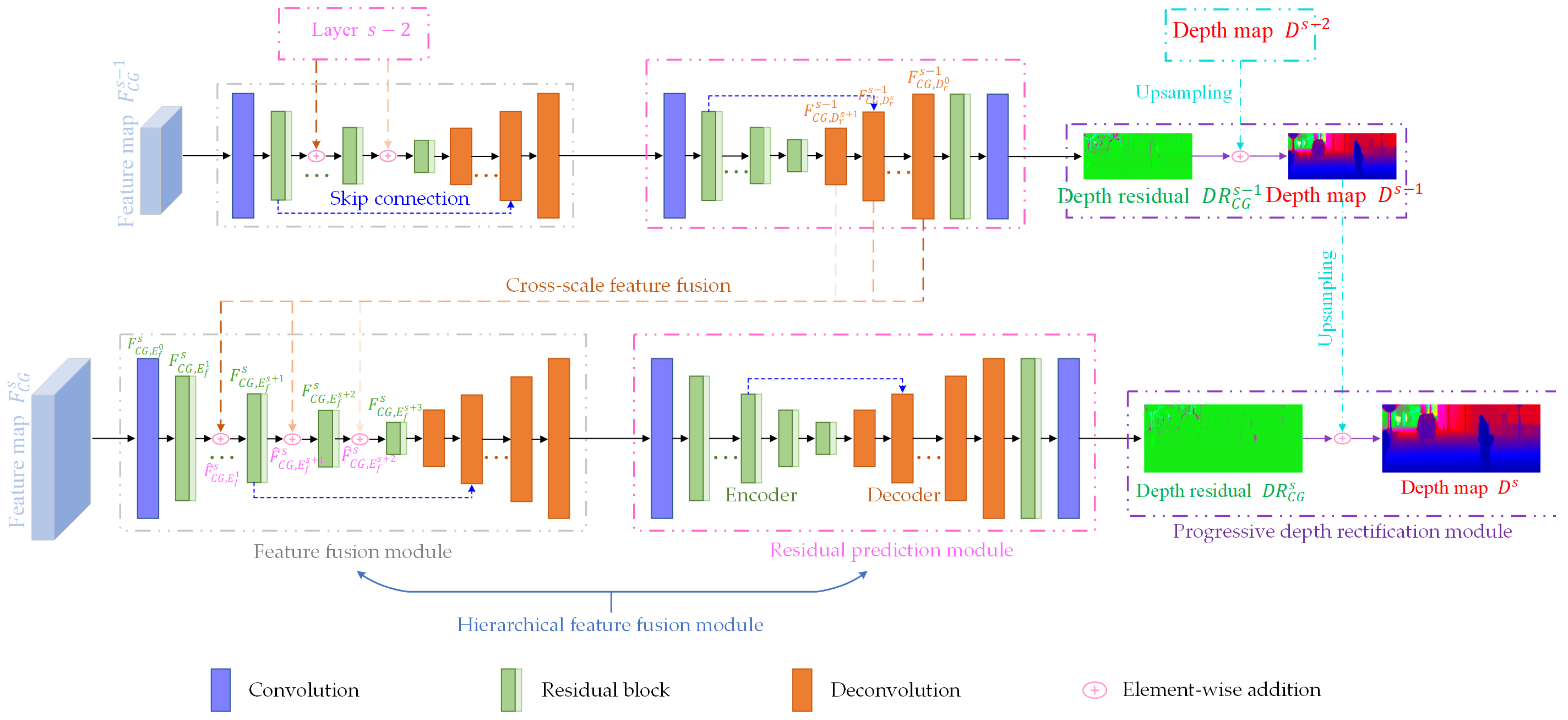
As shown in Figure 3, the hierarchical depth completion subnetwork is adopted to produce a robust initial depth map. The hierarchical feature fusion module that gradually fuses the multi-scale feature maps is used to generate an accurate depth residual map, and the progressive depth rectification module that gradually rectifies the low-resolution depth map by utilizing the generated high-resolution depth residual map is implemented to achieve high-quality depth map prediction.
For the s -th layer’s feature map F C G s ( s [ 1 , , N 1 ] ), the hierarchical feature fusion module that consists of the feature fusion module and residual prediction module is first applied to generate a robust depth residual map D R C G s . In the feature fusion module, the low-resolution hierarchical feature representations { F C G , D r j s 1 | j [ 0,1 , s + 1 ] } that are produced from the residual prediction module of the ( s 1 ) -th layer are progressively fused to enlarge the receptive field of the extracted high-resolution feature map. Specifically, in the encoding stage of the feature fusion module, a 3 × 3 2D convolution and s + 3 residual blocks with a stride of 2 (the structure of each residual block is shown in Table 1) are used to progressively extract the hierarchical feature representations { F C G , E f j s | j [ 0,1 , s + 3 ] } , where the channels of F C G , E f j s are 64. Note that the same-resolution hierarchical feature representations F C G , D r j s 1 ( j 0,1 , s + 1 ) are simultaneously fused to F C G , E f j s ( j [ 1,2 , , s + 2 ] ) to obtain more robust global feature representations F ^ C G , E f j s ( j [ 1,2 , , s + 2 ] ), which can be written as:
F ^ C G , E f j s = F C G , E f j s F C G , D r j 1 s 1
Subsequently, s + 3 deconvolutions with a skip connection operation are employed to decode the encoded hierarchical feature representations to generate a more robust feature map. For the residual prediction module, a 3 × 3 2D convolution and s + 3 residual blocks with a stride of 2 are also adopted to extract deeper contextual feature representations, and then s + 3 deconvolutions with a skip connection operation, a residual block, and a 3 × 3 2D convolution are applied to produce the accurate and reliable depth residual map D R C G s .
After obtaining D R C G s , the progressive depth rectification module is utilized to predict the accurate depth map D s . The main advantages of the progressive depth rectification module are twofold. For one thing, the low-resolution depth map D s 1 can provide abundant geometric structure prior information, integrating low-resolution depth maps can significantly improve the quality of predicted high-resolution depth map D s , especially for those areas with extremely sparse depth measurements. For another, it is difficult to prevent the detail loss of low-resolution depth map, thus the high-resolution depth residual map D R C G s generated by the hierarchical feature fusion module is required to recover the fine-grained geometry structure. Specifically, the depth prior is first obtained from the low-resolution depth map D s 1 using the bilinear interpolation function f U B s . , and then the depth prior is rectified utilizing the predicted depth residual D R C G s to produce the high-quality depth map D s , which can be written as:
D s = f U B s D s 1 D R C G s
The above process is repeated from the 1 -th layer to the ( N 1 ) -th layer to progressively generate the high-quality depth map D N 1 R H × W . However, for the lowest-resolution feature map F C G 0 , only the hierarchical feature fusion module is implemented to directly generate the lowest-resolution depth map D 0 .

3.3. MLSPN-Based Depth Map Refinement

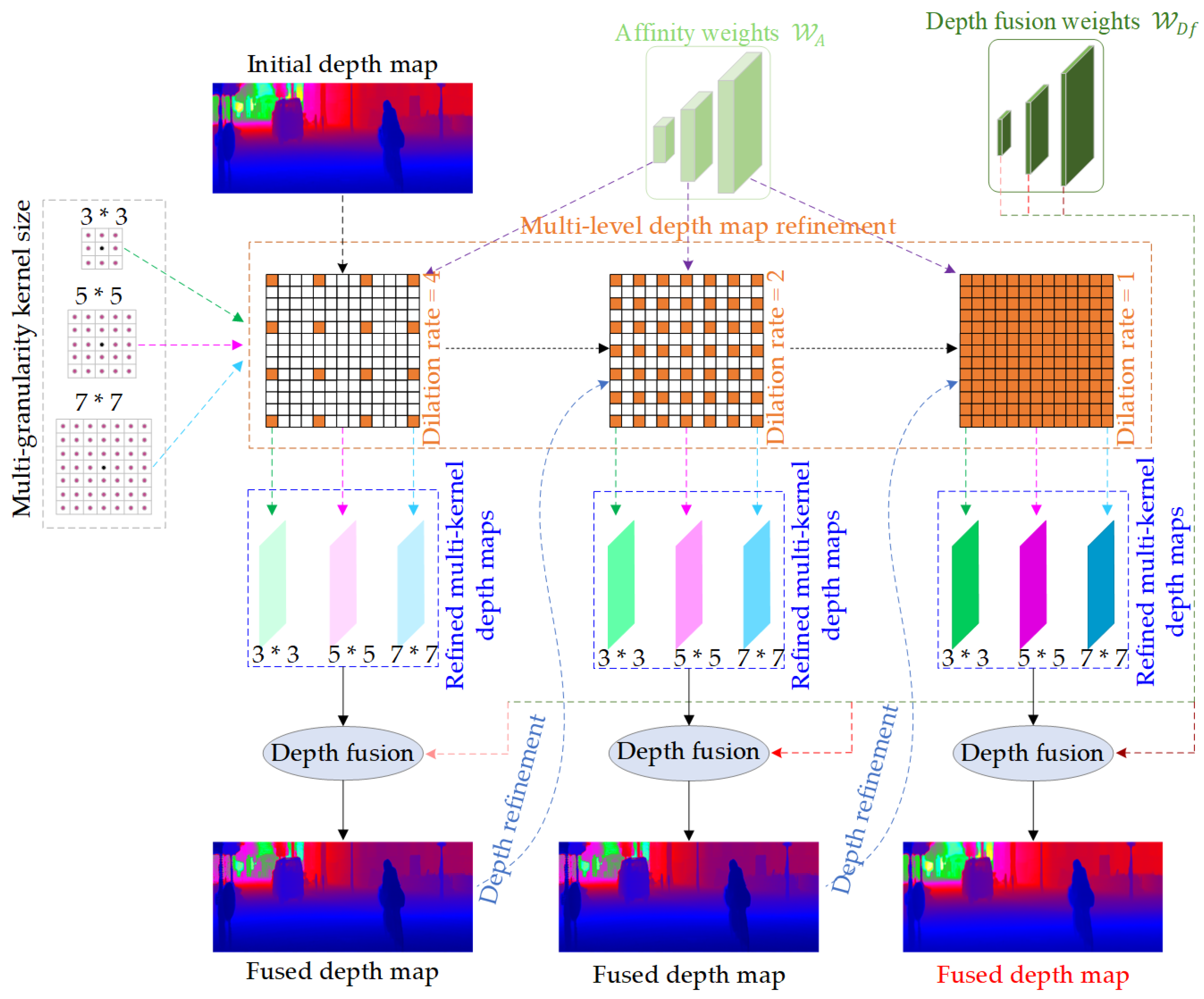
After obtaining the robust initial depth map D N 1 , the MLSPN-based depth map refinement subnetwork is also required to further refine D N 1 to recover more details, resulting in a state-of-the-art depth completion result. The detailed process of the MLSPN-based depth map refinement subnetwork is shown in Figure 4.
Let D 0 = D N 1 be the initial depth map, W A = W A l , k l 1,2 , 3 ,   a n d   k [ 1,2 , 3 ] } ( W A l , k R H 2 l 1 × W 2 l 1 × ( K k 2 1 ) ) and W D f = W D f l l [ 1,2 , 3 ] } ( W D f l R H 2 l 1 × W 2 l 1 × 3 ) are the multi-scale affinity and depth fusion weights that are produced from the original-resolution residual prediction module. K = { K ( k ) | k [ 1,2 , 3 ] } represents the multi-granularity convolutional transformation kernels, and the k -th kernel size is K k = 2 × k + 1 . D R = D R ( l ) l [ 1,2 , 3 ] } denotes the set of multi-level dilation rates, and the l -th level’s dilation rate is D R l = 2 l 1 . For the MLSPN-based depth map refinement subnetwork, the multi-level CSPN++ modules are iteratively applied to progressively obtain the high-quality depth map D ^ R e f . Specifically, for the l -th level’s CSPN++ module, the refined depth map D ^ 0 l + 1 (where D ^ 0 4 = D 0 ) of the ( l + 1 ) -th level is first split into D R l × D R l non-overlapping depth patches D S p a t c h l + 1 = D p a t c h m m [ 0,1 , , D R l × D R l 1 ] } according to the corresponding dilation rate D R l [22]. Subsequently, for each depth patch D p a t c h m D S p a t c h l + 1 , the refined multi-kernel depth patches D K p a t c h , T l m = D p a t c h , T l m , k k [ 1,2 , 3 ] } (as shown in Figure 4) can be yielded after T l = 2 × ( 4 l ) iterations as follows:
D p a t c h , t m , k u , v = w u , v l , k × D p a t c h , t 1 m , k u , v + i = k k j = k k w i , j l , k × D p a t c h , t 1 m , k u + i , v + j
where D K p a t c h , t m = D p a t c h , t m , k k [ 1,2 , 3 ] } represents the refined multi-kernel depth patches of the t -th iteration, D p a t c h , 0 m , k = D p a t c h m . p ( u , v ) denotes the pixel location, and q ( u + i , v + j ) stands for the adjacent pixel of pixel p in a K k × K k kernel. w u , v l , k and w i , j l , k are the weights used to adaptively adjust the contribution of the adjacent pixels’ depths of D p a t c h , t 1 m , k in refined depth patch D p a t c h , t m , k , which can be directly calculated from the affinity weights W A l , k as follows:
w i , j l , k = W A l , k u , v , c i , j i i = k k j j = k k W A l , k u , v , c i i , j j w u , v l , k = 1 i = k k j = k k w i , j l , k
where c i , j = i + k × 2 k + 1 + ( j + k ) . After obtaining the refined multi-kernel depth patches D K p a t c h , T l m , the fused depth patches D S ^ p a t c h l = D ^ p a t c h m m [ 0,1 , , D R l × D R l 1 ] } can be obtained as follows:
D ^ p a t c h m ( u , v ) = k = 1 3 D p a t c h , T l m , k ( u , v ) × W D f l ( u , v , k 1 ) k = 1 3 W D f l ( u , v , k 1 )
Finally, the fused depth patches D S ^ p a t c h l are merged to yield the refined depth map D ^ 0 l . The above process is iteratively implemented from level l = 3 to l = 1 to generate the high-quality depth map D ^ R e f = D ^ 0 1 .

3.4. Training Loss

As HFF-Net has multiple depth map outputs, the model parameters of HFF-Net are trained in an end-to-end manner using the following total loss function:
L f T o t a l = s = 0 N 1 λ H s × f L 2 D s + l = 1 3 λ R l × f L 2 D ^ 0 l
where λ H s and λ R l are the hyper parameters used to balance the contribution of each loss term in L f T o t a l . D s represents the predicted depth map from the hierarchical depth completion subnetwork of the s -th layer, and D ^ 0 l denotes the refined depth map of the l -th level’s CSPN++ module. f L 2 ( . ) is the widely used L 2 loss function [23], which can be defined as:
f L 2 D = 1 N P g t × p P g t D p D g t ( p ) 2
where D and D g t represent the predicted and the corresponding ground-truth depth maps, respectively. P g t denotes the set of valid depth pixels in D g t , and N P g t represents the number of pixels in P g t . Note that, if D and D g t have different resolutions, the nearest neighbor interpolation operation is first used to downsample D g t to the same resolution as D , and then the corresponding L 2 loss is calculated by Equation (8).

4. Experiments and Analysis

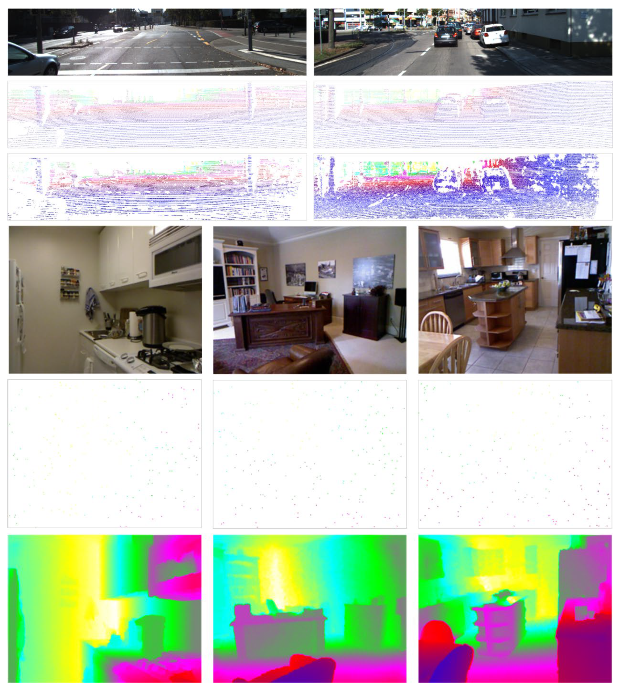
Comprehensive experiments were undertaken on both the outdoor KITTI DC dataset [8] and the indoor NYUv2 dataset [19] to validate the performance of HFF-Net. As shown in Table 2, the KITTI DC dataset is a high-resolution real-world autonomous driving dataset that provides 86,898 frames for the training set (of which 85,898 and 1000 frames are for model training and validation, respectively) and 1000 frames for the test set. The sparse depth maps (about 6% valid depth pixels) were generated from the synchronized and calibrated LiDAR point cloud that was captured by a Velodyne HDL-64E laser scanner (Velodyne Lidar, San Jose, USA), and the ground-truth depth maps (about 16% valid depth pixels) were obtained from the LiDAR point cloud that was collected by registering 11 consecutive temporal LiDAR scan frames into one. The resolution of the training and test sets (i.e., the RGB images, sparse depth maps, and ground-truth depth maps) were top-cropped and center-cropped to 1216 × 256 pixels because there were nearly no LiDAR projections for the top 100 pixels. The NYUv2 dataset contains 464 indoor scenes, and the image pairs (where each pair includes an RGB image and the corresponding dense ground-truth depth map of each scene were captured using a Microsoft Kinect sensor (Microsoft, Redmond and Washington, USA) [66]. The training set consists of 47,584 image pairs that were uniformly sampled from 249 scenes, and the test set comprises 654 image pairs sampled from the remaining 215 scenes. Following the common settings of the previous depth completion algorithms [1,21,62], the resolutions of both the training and test sets were downsampled to 320 × 240 pixels, and then further center-cropped to 304 × 228 pixels. For each image pair, the sparse depth map was produced from the corresponding dense ground-truth depth map by randomly sampling 500 pixels. Some representative scenes of the KITTI DC and NYUv2 datasets are shown in Figure 5. Note that, in this paper, the depth values of all the depth maps from small to large were mapped to the pseudo-color from blue to yellow.
In the experiments, the following nine evaluation metrics [1,55,56] were adopted to evaluate the quality of the depth completion results, i.e., the root-mean-square error (RMSE), the mean absolute error (MAE), the root-mean-square error of the inverse depth (iRMSE), the mean absolute error of the inverse depth (iMAE), the mean absolute relative error (REL), and δ i (the percentage of pixels whose relative depth errors are less than a given threshold i , where i [ 1.25 , 1.25 2 , 1.25 3 ] ). These metrics are calculated as follows:
R M S E = 1 N P g t × p P g t D p D g t ( p ) 2 M A E = 1 N P g t × p P g t D p D g t ( p ) i R M S E = 1 N P g t × p P g t 1 D ( p ) 1 D g t ( p ) 2 i M A E = 1 N P g t × p P g t 1 D ( p ) 1 D g t ( p ) R E L = 1 N P g t × p P g t D p D g t ( p ) D g t ( p ) δ i = 100 % × 1 N P g t × p P g t [ m a x D p D g t p , D g t p D p < i ]
where [ . ] denotes the element-wise Iverson bracket [67]. Note that the RMSE score is the primary metric used to evaluate the quality of the predicted dense depth map since it is sensitive to large errors, and the other metrics can be used to reveal some specific properties.

4.1. Implementation Details

The HFF-Net model was trained using an NVIDIA RTX 3090 GPU (NVIDIA, Santa Clara, CA, USA) with the PyTorch 1.12 architecture. In the experiments, the AdamW optimizer ( β 1 = 0.9 , β 2 = 0.999 ) [68] was employed to train the end-to-end HFF-Net architecture in a fully supervised manner, and the hyper parameters ( λ H 0 , λ H 1 , λ H 2 , λ R 3 , λ R 2 , λ R 1 ) of Equation (7) were empirically set to (0.1, 0.1, 0.2, 0, 0, 1.0). To obtain robust model parameters, a three-stage training strategy [22,69] was adopted. That is, the hierarchical depth completion subnetwork was first trained, and then the remaining MLSPN-based depth map refinement subnetwork was trained. Finally, the entire HFF-Net architecture was trained to obtain the optimized model parameters. For each training stage (as shown in Table 2), the model was trained for 30 epochs with a batch size of 3 and 100 epochs with a batch size of 12 for the KITTI DC and NYUv2 datasets, respectively. The initial learning rate was set to 0.001. The learning rate was then reduced by half in epochs 5, 10, 15, 20, and 25 for the KITTI DC dataset, and reduced by half in epochs 36, 48, 60, 72, and 84 for the NYUv2 dataset.

4.2. Quantitative Evaluation

We first compared the performance of HFF-Net with that of several state-of-the-art methods on both the KITTI DC and NYUv2 datasets. The quantitative evaluation results for the predicted dense depth maps are provided in Table 3 and Table 4. As summarized in Table 3 and Table 4, the RMSE, MAE, iRMSE, and iMAE values of HFF-Net are 694.90 mm, 201.54 mm, 1.95/km, and 0.88/km, respectively, for the KITTI DC test set, and the RMSE, REL, σ 1.25 , δ 1.25 2 , and δ 1.25 3 scores are 0.093 m, 0.013, 99.6%, 99.9%, and 100.0%, respectively, for the NYUv2 test set. This demonstrates that, in terms of the primary RMSE score, HFF-Net achieves the best depth prediction results on the KITTI DC test set, while simultaneously obtaining competitive results for the NYUv2 dataset.
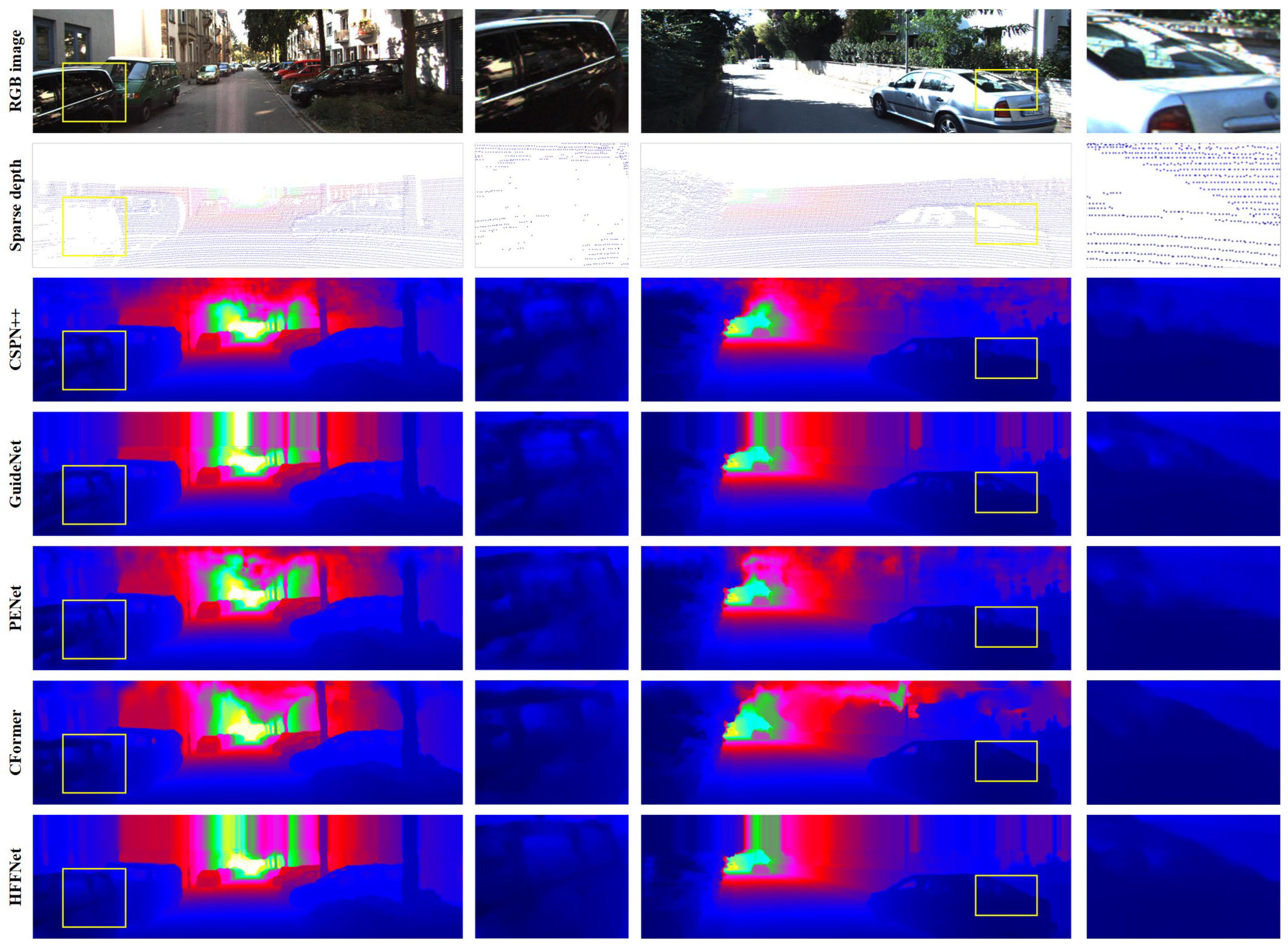
As reported in Table 3 and Table 4, it can be seen that HFF-Net has greater advantages over NLSPN, CFormer, and LRRU on the KITTI DC dataset, but the reverse results are produced for the NYUv2 dataset. The reason for this is that the KITTI DC dataset was captured in a more complex outdoor environment with uncontrollable lighting conditions and has a higher image resolution. As a result, for the high-resolution KITTI DC dataset, fusing multi-scale low-resolution feature representations can significantly improve the robustness of the original-resolution feature representations to achieve more accurate and reliable depth completion results. However, for the low-resolution indoor NYUv2 dataset, the original-resolution feature representations can provide abundant contextual information, and thus the hierarchical depth completion subnetwork and MLSPN-based depth map refinement subnetwork do not prominently boost the quality of the completed depth map. In addition, it can also be found that HFF-Net obtains better results than CSPN and CSPN++. Figure 6 and Figure 7 provide a qualitative comparison of the depth completion results for some representative scenes in both the KITTI DC and NYUv2 datasets. As shown in the rectangular regions in Figure 6 and Figure 7, it can be found that HFF-Net obtains better depth prediction results than the other comparison methods for those areas that have extremely sparse depth measurements. The reasons for this are twofold. For one thing, the low-resolution feature representations contain higher-level geometric and semantic information, and thus fusing low-resolution feature representations will ensure that these pixels within the areas that have extremely sparse depth measurements obtain more abundant long-range dependencies to produce a more robust initial dense depth map, multi-level affinity weights, and depth fusion weights. For another thing, the MLSPN-based depth map refinement subnetwork is adopted, which iteratively refines the initial depth map in a coarse-to-fine manner to avoid the predicted depth map being trapped in local minima for areas with extremely sparse depth measurements, resulting in state-of-the-art depth completion results.

4.3. Discussion

4.3.1. Ablation Study

As described in Section 3, HFF-Net contains two key parts: the hierarchical depth completion architecture for generating a robust initial depth map, and the MLSPN-based depth refinement subnetwork to iteratively refine the initial depth map to achieve state-of-the-art depth completion results. To analyze the importance of each component of HFF-Net, the following seven model variants are compared: (1) Baseline, which directly predicts the dense depth map from the hierarchical depth completion subnetwork without fusing the multi-scale feature maps; (2) Model-Net1, Model-Net2, and Model-Net3, which fuse multiple different-scale feature representations; and (3) Model-Net4, Model-Net5, and HFF-Net, which simultaneously integrate multi-scale feature fusion and MLSPN-based depth map refinement strategies. Note that, for the MLSPN-based depth refinement subnetwork, the iteration numbers for D R 1 , { D R 1 , D R 2 }, and { D R 1 , D R 2 , D R 3 } for Model-Net4, Model-Net5, and HFF-Net were set to 12, {6, 6}, and {6, 4, 2}, respectively. In addition, the KITTI DC dataset was used in the ablation experiments since it provides sparse depth maps and is more representative of a real-world environment. Table 5 and Figure 8 show the quantitative and qualitative depth completion results of the different model variants on the KITTI DC validation set.
As reported in Table 4, for the hierarchical depth completion subnetwork, the RMSE score of the predicted depth maps gradually decreases as more low-resolution feature representations are fused, while rapidly increasing after reaching the lowest point. This indicates that the multi-scale feature fusion strategy can significantly improve the quality of the predicted depth maps, and the best results are obtained when fusing the three different-scale feature representations, as exhibited in Model-Net2 in Table 5. It can also be found that the RMSE scores of Model-Net5 and HFF-Net are lower than those of Model-Net4, and HFF-Net with three different-level SPNs obtains the best performance. The reason for this is that the MLSPN-based depth refinement subnetwork can yield better results than a single-level SPN [24] since the low-resolution affinity weights can provide reliable long-range contextual information to prevent depth ambiguities in the refined depth map in large areas where depth measurements are extremely sparse. Figure 8 provides a qualitative comparison of the predicted depth maps for some representative scenes. As displayed in the black rectangle regions in Figure 8, the quality of the predicted maps for the large regions with extremely sparse depth measurements is improved when fusing the low-resolution feature representations. Furthermore, the MLSPN-based depth map refinement subnetwork with three levels can obtain better results than a subnetwork with only a single or two levels.

4.3.2. Comparison with Different-Level Sparsity Measurements

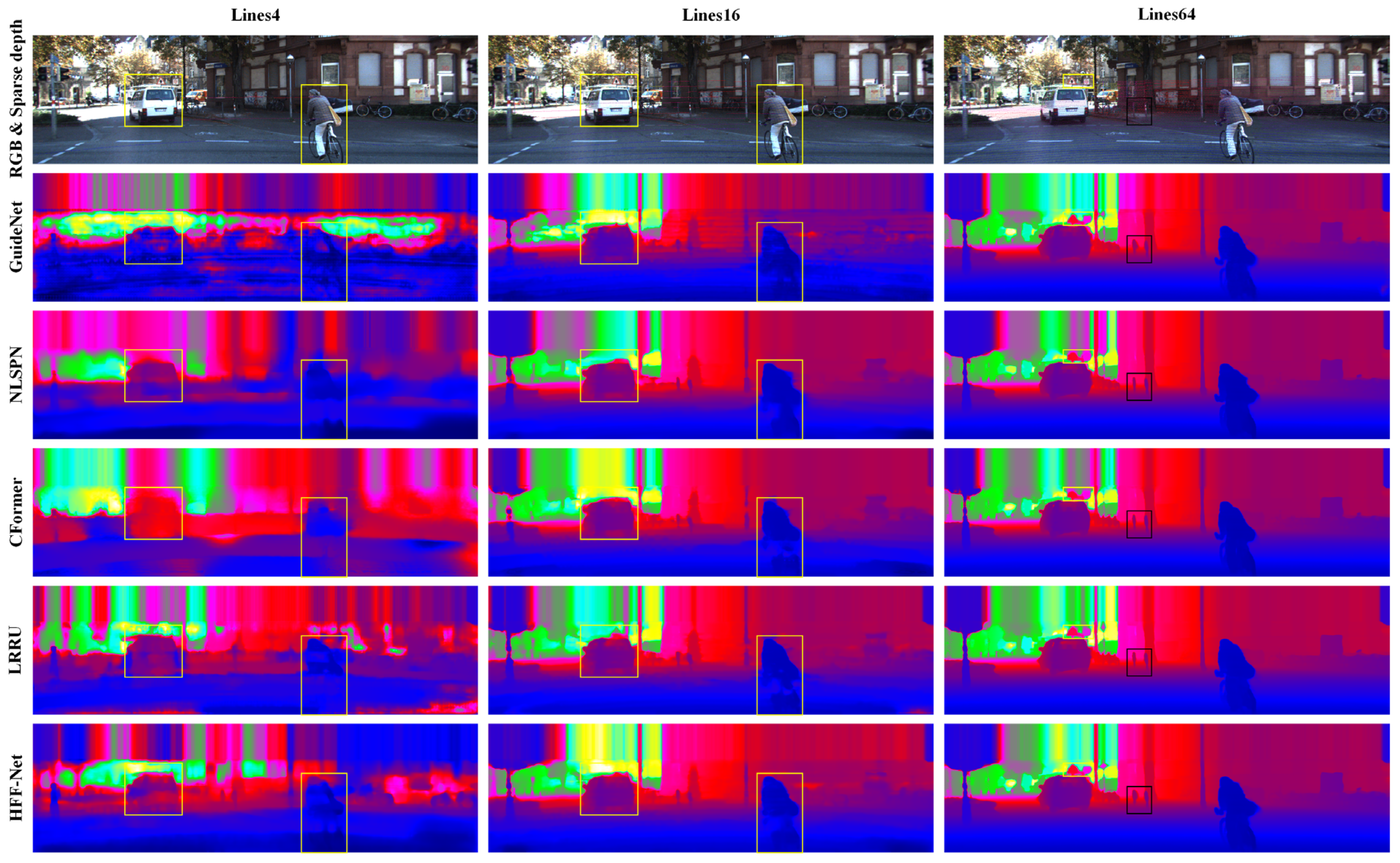
In general, good depth completion architecture should have the ability to be suitable for different-level sparsity measurements. To validate the robustness of HFF-Net at different-level sparse depth representations, we first trained HFF-Net on the 64-line LiDAR depth maps of the KITTI DC training set, and then tested its performance on the validation set across various sparsity levels that were obtained by referring to Zhao et al. [72]. For a fair comparison, all the comparison methods were retrained with the same parameter settings, including the optimizer, training epochs, and learning rate. Table 6 and Figure 9 provide the quantitative and qualitative comparison results.
As shown in Table 6, HFF-Net can obtain superior depth completion results at almost all the sparsity levels in terms of the RMSE score. This indicates that fusing the multi-scale feature representations can ensure that HFF-Net learns more global contextual information to achieve accurate and reliable depth completion results. Furthermore, it can also be found that the depth completion quality of GuideNet is significantly lower than that of the comparison methods for the sparser levels of the 8-line, 4-line, and 1-line scenarios. This demonstrates that the SPN-based depth refinement strategy is essential for producing state-of-the-art depth completion results. Meanwhile, as exhibited in the yellow rectangle regions in Figure 9, HFF-Net has greater advantages in preventing depth ambiguities in areas with extremely sparse depth measurements. The reason for this is that the low-resolution feature representations can provide reliable long-range dependencies for extremely sparse depth measurements, and thus a more robust initial depth map and affinity weights can be obtained by progressively fusing the low-resolution feature representations. In addition, the MLSPN-based depth map refinement subnetwork is adopted, which utilizes the robust multi-scale affinity weights to further refine the predicted initial depth map in a coarse-to-fine manner to achieve high-quality depth map reconstruction. However, as shown in the black regions in Figure 9, when fusing the low-resolution feature representations, the details and boundary features are lost. In our future work, we will explore more effective strategies to overcome this limitation to further improve the quality of the predicted depth map.

4.3.3. Zero-Shot Generalization Ability

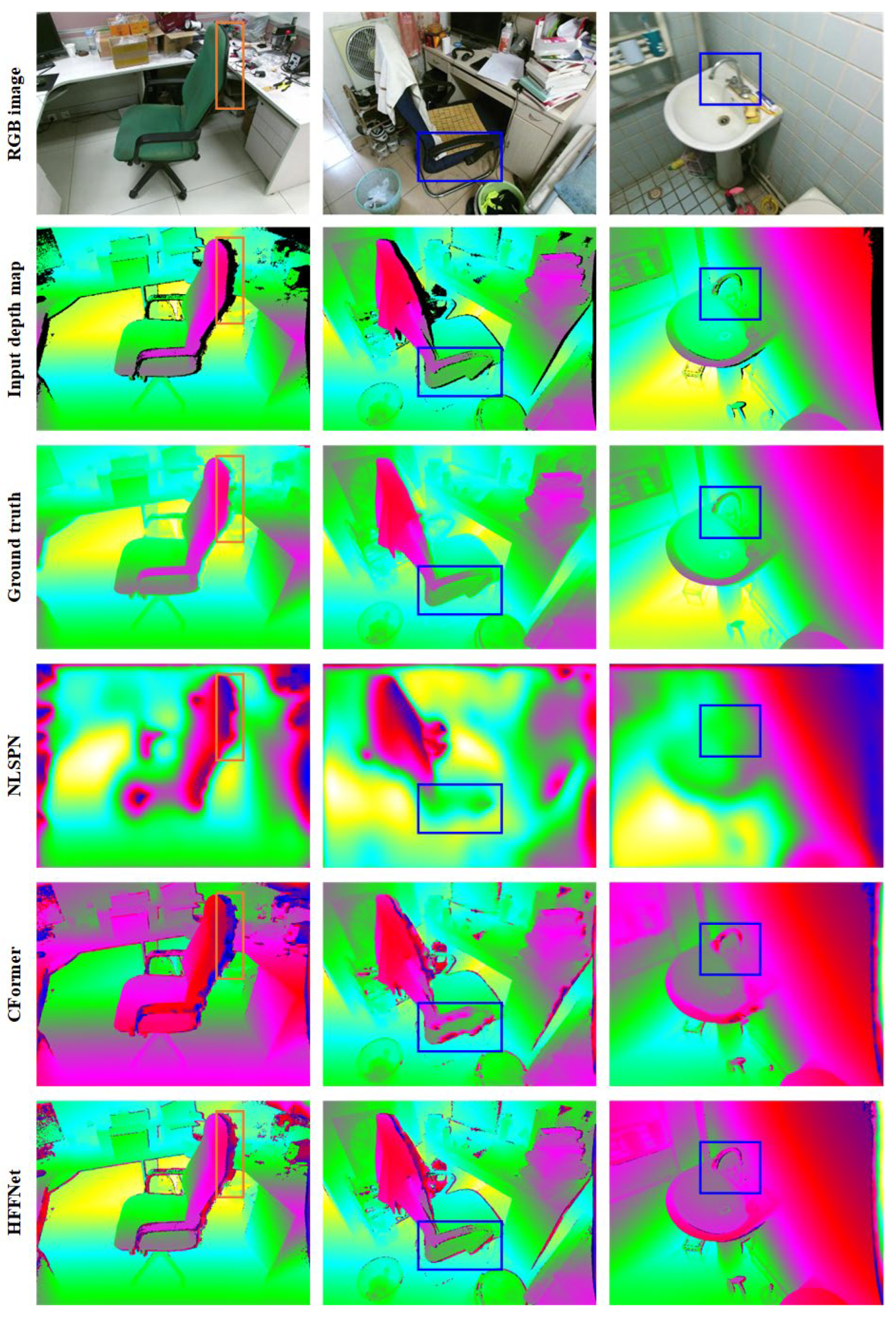
The indoor SUN RGB-D test set [73] was used to validate the zero-shot generalization performance of the proposed HFF-Net architecture. For the SUN RGB-D test set, which consists of 5050 image pairs (where each image pair contains an RGB image and the corresponding synchronized depth map) captured by Microsoft Kinect sensors, and the image resolution is 640 × 480 pixels. Similarly to the method of SparseDC [18], in the experiments, we used the synchronized depth maps as sparse depth maps, and the inpainted depth maps as ground truths. Meanwhile, the pre-trained models on the NYUv2 dataset were directly used to quantitatively and qualitatively compare the generalization performance of HFF-Net and some representative methods (i.e., NLSPN and CFormer). As shown in Table 7, the RMSE and REL scores of HFF-Net are 0.490m and 0.109 for the SUN RGB-D test set, respectively. This reveals that HFF-Net has better generalization performance for unseen environments. In addition, we can also find that HFF-Net has fewer model parameters than NLSPN and CFormer architectures. Figure 10 further shows the qualitative comparison of the completed depth maps of some representative scenes on the SUN RGB-D test set. As reported in the blue rectangular regions in Figure 10, which also indicates that HFF-Net can produce better depth completion results.
Although HFF-Net can achieve higher-quality depth completion results than those of the comparison methods, the following limitations remain. On the one hand, HFF-Net has larger memory consumption (as shown in Table 7) than that of NLSPN and CFormer architectures, and its runtime needs to be further decreased to meet real-time requirements. On the other hand, HFF-Net still struggles to achieve the correct depth completion results for depth discontinuity areas, as shown in the orange rectangular regions in Figure 10. In our future work, we will explore more effective strategies to overcome the aforementioned limitations.

5. Conclusions

In this paper, we have presented a novel hierarchical feature fusion network (HFF-Net) for achieving accurate and reliable depth completion results. The main advantages of HFF-Net are the hierarchical depth completion subnetwork that progressively fuses multi-scale feature representations to significantly improve the quality of the predicted initial depth map and the multi-level affinity and depth fusion weights, and the MLSPN-based depth map refinement subnetwork that extends the CSPN into a coarse-to-fine multi-level space and simultaneously utilizes more robust multi-level affinity weights to reduce the depth ambiguities of the refined depth map in large areas with extremely sparse depth measurements. The high-resolution outdoor KITTI DC and close-range indoor NYUv2 datasets were used to validate the performance of the HFF-Net architecture, and the comprehensive experimental results confirmed that HFF-Net can obtain state-of-the-art depth completion results on both the KITTI DC and NYUv2 datasets. It was also found that HFF-Net has greater advantages than the existing single-scale depth completion architectures in areas with extremely sparse depth measurements, as more long-range dependencies can be obtained by adaptively fusing the low-resolution feature representations. However, the main shortcomings of HFF-Net are the boundary ambiguities of the predicted depth map due to the irregular and sparse depth measurements. In the future, we plan to explore whether integrating an edge feature extraction subnetwork [42] into the HFF-Net architecture could reduce the problem of blurred boundaries. In addition, for the irregular, sparse depth map, the hierarchical feature extraction subnetwork may not be able to extract robust feature representations by adopting spatially invariant convolution, so we will also consider replacing this with a sparse convolutional layer [8] to extract a more robust feature representation.

Author Contributions

Conceptualization, Mao Tian; methodology, Yi Han and Mao Tian; software, Qiaosheng Li and Yi Han; validation, Mao Tian, Yi Han, Qiaosheng Li and Wuyang Shan; formal analysis, Yi Han, Qiaosheng Li and Wuyang Shan; investigation, Mao Tian, Yi Han, Qiaosheng Li; resources, Qiaosheng Li and Wuyang Shan; data curation, Yi Han and Mao Tian; writing—original draft preparation, Yi Han, Qiaosheng Li and Mao Tian; writing—review and editing, Mao Tian; visualization, Yi Han, Qiaosheng Li and Wuyang Shan; supervision, Mao Tian; project administration, Mao Tian; funding acquisition, Mao Tian. All authors have read and agreed to the published version of the manuscript.

Funding

This research was funded by the National Natural Science Foundation of China (No. 42001417); the Science and Technology Research Program of Chongqing Municipal Education Commission (No. KJQN202300647).

Data Availability Statement

The original contributions presented in the study are included in the article, further inquiries can be directed to the corresponding author.

Acknowledgments

The authors would first like to acknowledge the Editor-in-Chief, Associate Editor, and anonymous reviewers for their valuable feedback. We would also like to thank the Karlsruhe Institute of Technology, the Toyota Technological Institute at Chicago, and the Computer Science at New York University’s Courant Institute for providing the corresponding benchmark datasets.

Conflicts of Interest

The authors declare no conflicts of interest.

References

  1. Wang, Y.; Li, B.; Zhang, G.; Liu, Q.; Gao, T.; Dai, Y. LRRU: Long-short Range Recurrent Updating Networks for Depth Completion. In Proceedings of the IEEE/CVF International Conference on Computer Vision, Paris, France, 1–6 October 2023; pp. 9422–9432. [Google Scholar]
  2. Chen, Z.; Li, W.; Cui, Z.; Zhang, Y. Surface depth estimation from multi-view stereo satellite images with distribution contrast network. IEEE J. Sel. Top. Appl. Earth Obs. Remote Sens. 2024, 17, 17837–17845. [Google Scholar] [CrossRef]
  3. Hu, P.; Yang, B.; Dong, Z.; Yuan, P.; Huang, R.; Fan, H.; Sun, X. Towards reconstructing 3D buildings from ALS data based on gestalt laws. Remote Sens. 2018, 10, 1127. [Google Scholar] [CrossRef]
  4. Han, X.; Liu, C.; Zhou, Y.; Tan, K.; Dong, Z.; Yang, B. WHU-Urban3D: An urban scene LiDAR point cloud dataset for semantic instance segmentation. ISPRS J. Photogramm. Remote Sens. 2024, 209, 500–513. [Google Scholar] [CrossRef]
  5. Chen, C.; Jin, A.; Wang, Z.; Zheng, Y.; Yang, B.; Zhou, J.; Xu, Y.; Tu, Z. SGSR-Net: Structure Semantics Guided LiDAR Super-Resolution Network for Indoor LiDAR SLAM. IEEE Trans. Multimed. 2023, 26, 1842–1854. [Google Scholar] [CrossRef]
  6. Yan, Z.; Wang, K.; Li, X.; Zhang, Z.; Li, G.; Li, J.; Yang, J. Learning complementary correlations for depth super-resolution with incomplete data in real world. IEEE Trans. Neural Netw. Learn. Syst. 2022, 35, 5616–5626. [Google Scholar] [CrossRef] [PubMed]
  7. Thiel, K.; Wehr, A. Performance capabilities of laser scanners–an overview and measurement principle analysis. Int. Arch. Photogramm. Remote Sens. Spat. Inf. Sci. 2004, 36, 14–18. [Google Scholar]
  8. Uhrig, J.; Schneider, N.; Schneider, L.; Franke, U.; Brox, T.; Geiger, A. Sparsity invariant cnns. In Proceedings of the 2017 International Conference on 3D Vision (3DV), Qingdao, China, 10–12 October 2017; IEEE: Piscataway, NJ, USA, 2017; pp. 11–20. [Google Scholar]
  9. Yin, W.; Liu, Y.; Shen, C. Virtual normal: Enforcing geometric constraints for accurate and robust depth prediction. IEEE Trans. Pattern Anal. Mach. Intell. 2021, 44, 7282–7295. [Google Scholar] [CrossRef]
  10. Yin, W.; Zhang, C.; Chen, H.; Cai, Z.; Yu, G.; Wang, K.; Chen, X.; Shen, C. Metric3d: Towards zero-shot metric 3d prediction from a single image. In Proceedings of the IEEE/CVF International Conference on Computer Vision, Paris, France, 1–6 October 2023; pp. 9043–9053. [Google Scholar]
  11. Yao, Y.; Luo, Z.; Li, S.; Fang, T.; Quan, L. Mvsnet: Depth inference for unstructured multi-view stereo. In Proceedings of the European Conference on Computer Vision (ECCV), Munich, Germany, 8–14 September 2018; pp. 767–783. [Google Scholar]
  12. Chang, J.; Chen, Y. Pyramid Stereo Matching Network. In Proceedings of the IEEE/CVF Conference on Computer Vision and Pattern Recognition (CVPR), Salt Lake City, UT, USA, 18–22 June 2018; pp. 5410–5418. [Google Scholar]
  13. Jiang, L.; Wang, F.; Zhang, W.; Li, P.; You, H.; Xiang, Y. Rethinking the Key Factors for the Generalization of Remote Sensing Stereo Matching Networks. IEEE J. Sel. Top. Appl. Earth Obs. Remote Sens. 2024, 18, 4936–4948. [Google Scholar] [CrossRef]
  14. Zuo, Y.; Deng, J. OGNI-DC: Robust Depth Completion with Optimization-Guided Neural Iterations. arXiv 2024, arXiv:2406.11711. [Google Scholar]
  15. Min, D.; Lu, J.; Do, M.N. Depth video enhancement based on weighted mode filtering. IEEE Trans. Image Process. 2011, 21, 1176–1190. [Google Scholar] [CrossRef]
  16. Zhang, Y.; Feng, Y.; Liu, X.; Zhai, D.; Ji, X.; Wang, H.; Dai, Q. Color-guided depth image recovery with adaptive data fidelity and transferred graph Laplacian regularization. IEEE Trans. Circuits Syst. Video Technol. 2019, 30, 320–333. [Google Scholar] [CrossRef]
  17. Zhang, Y.; Guo, X.; Poggi, M.; Zhu, Z.; Huang, G.; Mattoccia, S. Completionformer: Depth completion with convolutions and vision transformers. In Proceedings of the IEEE/CVF Conference on Computer Vision and Pattern Recognition, Vancouver, BC, Canada, 17–24 June 2023; pp. 18527–18536. [Google Scholar]
  18. Long, C.; Zhang, W.; Chen, Z.; Wang, H.; Liu, Y.; Tong, P.; Cao, Z.; Dong, Z.; Yang, B. SparseDC: Depth Completion from sparse and non-uniform inputs. Inf. Fusion 2024, 110, 102470. [Google Scholar] [CrossRef]
  19. Silberman, N.; Hoiem, D.; Kohli, P.; Fergus, R. Indoor segmentation and support inference from rgbd images. In Proceedings of the Computer Vision–ECCV 2012: 12th European Conference on Computer Vision, Florence, Italy, 7–13 October 2012; Proceedings, Part V 12. Springer: Berlin/Heidelberg, Germany, 2012; pp. 746–760. [Google Scholar]
  20. Cheng, X.; Wang, P.; Yang, R. Learning depth with convolutional spatial propagation network. IEEE Trans. Pattern Anal. Mach. Intell. 2019, 42, 2361–2379. [Google Scholar] [CrossRef] [PubMed]
  21. Park, J.; Joo, K.; Hu, Z.; Liu, C.-K.; Kweon, I.S. Non-local spatial propagation network for depth completion. In Proceedings of the Computer Vision–ECCV 2020: 16th European Conference, Glasgow, UK, 23–28 August 2020; Proceedings, Part XIII 16. Springer: Berlin/Heidelberg, Germany, 2020; pp. 120–136. [Google Scholar]
  22. Hu, M.; Wang, S.; Li, B.; Ning, S.; Fan, L.; Gong, X. Penet: Towards precise and efficient image guided depth completion. In Proceedings of the 2021 IEEE International Conference on Robotics and Automation (ICRA), Xi’an, China, 30 May–5 June 2021; IEEE: Piscataway, NJ, USA, 2021; pp. 13656–13662. [Google Scholar]
  23. Tang, J.; Tian, F.-P.; An, B.; Li, J.; Tan, P. Bilateral Propagation Network for Depth Completion. arXiv 2024, arXiv:2403.11270. [Google Scholar]
  24. Cheng, X.; Wang, P.; Guan, C.; Yang, R. Cspn++: Learning context and resource aware convolutional spatial propagation networks for depth completion. In Proceedings of the AAAI Conference on Artificial Intelligence, New York, NY, USA, 7–12 February 2020; Volume 34, pp. 10615–10622. [Google Scholar]
  25. Carion, N.; Massa, F.; Synnaeve, G.; Usunier, N.; Kirillov, A.; Zagoruyko, S. End-to-end object detection with transformers. In Proceedings of the European Conference on Computer Vision, Glasgow, UK, 23–28 August 2020; Springer: Berlin/Heidelberg, Germany, 2020; pp. 213–229. [Google Scholar]
  26. Cheng, X.; Wang, P.; Yang, R. Depth estimation via affinity learned with convolutional spatial propagation network. In Proceedings of the European Conference on Computer Vision (ECCV), Munich, Germany, 8–14 September 2018; pp. 103–119. [Google Scholar]
  27. Kendall, A.; Martirosyan, H.; Dasgupta, S.; Henry, P. End-to-End Learning of Geometry and Context for Deep Stereo Regression. In Proceedings of the International Conference on Computer Vision, Venice, Italy, 22–29 October 2017; pp. 66–75. [Google Scholar]
  28. Xu, Z.; Jiang, Y.; Wang, J.; Wang, Y. A Dual Branch Multi-scale Stereo Matching Network for High-resolution Satellite Remote Sensing Images. IEEE J. Sel. Top. Appl. Earth Obs. Remote Sens. 2024, 18, 949–964. [Google Scholar] [CrossRef]
  29. Wang, K.; Yan, Z.; Fan, J.; Li, J.; Yang, J. Learning Inverse Laplacian Pyramid for Progressive Depth Completion. arXiv 2025, arXiv:2502.07289. [Google Scholar]
  30. He, S.; Li, S.; Jiang, S.; Jiang, W. HMSM-Net: Hierarchical multi-scale matching network for disparity estimation of high-resolution satellite stereo images. ISPRS J. Photogramm. Remote Sens. 2022, 188, 314–330. [Google Scholar] [CrossRef]
  31. Gu, X.; Fan, Z.; Zhu, S.; Dai, Z.; Tan, F.; Tan, P. Cascade cost volume for high-resolution multi-view stereo and stereo matching. In Proceedings of the IEEE/CVF Conference on Computer Vision and Pattern Recognition, Seattle, WA, USA, 13–19 June 2020; pp. 2495–2504. [Google Scholar]
  32. Saxena, A.; Chung, S.; Ng, A. Learning depth from single monocular images. Adv. Neural Inf. Process. Syst. 2005, 18, 1161–1168. [Google Scholar]
  33. Liu, B.; Gould, S.; Koller, D. Single image depth estimation from predicted semantic labels. In Proceedings of the 2010 IEEE Computer Society Conference on Computer Vision and Pattern Recognition, San Francisco, CA, USA, 13–18 June 2010; IEEE: Piscataway, NJ, USA, 2010; pp. 1253–1260. [Google Scholar]
  34. Ladicky, L.; Shi, J.; Pollefeys, M. Pulling things out of perspective. In Proceedings of the IEEE Conference on Computer Vision and Pattern Recognition, Columbus, OH, USA, 23–28 June 2014; pp. 89–96. [Google Scholar]
  35. Eigen, D.; Puhrsch, C.; Fergus, R. Depth map prediction from a single image using a multi-scale deep network. Adv. Neural Inf. Process. Syst. 2014, 27, 2366–2374. [Google Scholar]
  36. Eigen, D.; Fergus, R. Predicting depth, surface normals and semantic labels with a common multi-scale convolutional architecture. In Proceedings of the IEEE International Conference on Computer Vision, Santiago, Chile, 7–13 December 2015; pp. 2650–2658. [Google Scholar]
  37. Wang, K.; Yan, Z.; Fan, J.; Zhu, W.; Li, X.; Li, J.; Yang, J. Dcdepth: Progressive monocular depth estimation in discrete cosine domain. Adv. Neural Inf. Process. Syst. 2024, 37, 64629–64648. [Google Scholar]
  38. Yang, L.; Kang, B.; Huang, Z.; Xu, X.; Feng, J.; Zhao, H. Depth anything: Unleashing the power of large-scale unlabeled data. In Proceedings of the IEEE/CVF Conference on Computer Vision and Pattern Recognition, Seattle, WA, USA, 16–22 June 2024; pp. 10371–10381. [Google Scholar]
  39. Hartley, R.; Zisserman, A. Multiple View Geometry in Computer Vision; Cambridge University Press: Cambridge, UK, 2003. [Google Scholar]
  40. Yao, Y.; Luo, Z.; Li, S.; Shen, T.; Fang, T.; Quan, L. Recurrent MVSNet for High-Resolution Multi-View Stereo Depth Inference. In Proceedings of the Computer Vision and Pattern Recognition, Long Beach, CA, USA, 16–17 June 2019; pp. 5525–5534. [Google Scholar]
  41. Wang, X.; Xu, G.; Jia, H.; Yang, X. Selective-Stereo: Adaptive Frequency Information Selection for Stereo Matching. arXiv 2024, arXiv:2403.00486. [Google Scholar]
  42. Zhang, S.; Wei, Z.; Xu, W.; Zhang, L.; Wang, Y.; Zhang, J.; Liu, J. Edge aware depth inference for large-scale aerial building multi-view stereo. ISPRS J. Photogramm. Remote Sens. 2024, 207, 27–42. [Google Scholar] [CrossRef]
  43. Zbontar, J.; Lecun, Y. Computing the stereo matching cost with a convolutional neural network. In Proceedings of the Computer Vision and Pattern Recognition, Boston, MA, USA, 7–12 June 2015; pp. 1592–1599. [Google Scholar]
  44. Hirschmuller, H.; Scharstein, D. Evaluation of Stereo Matching Costs on Images with Radiometric Differences. IEEE Trans. Pattern Anal. Mach. Intell. 2009, 31, 1582–1599. [Google Scholar] [CrossRef] [PubMed]
  45. Rho, K.; Ha, J.; Kim, Y. Guideformer: Transformers for image guided depth completion. In Proceedings of the IEEE/CVF Conference on Computer Vision and Pattern Recognition, New Orleans, LA, USA, 18–24 June 2022; pp. 6250–6259. [Google Scholar]
  46. Liu, L.-K.; Chan, S.H.; Nguyen, T.Q. Depth reconstruction from sparse samples: Representation, algorithm, and sampling. IEEE Trans. Image Process. 2015, 24, 1983–1996. [Google Scholar] [CrossRef] [PubMed]
  47. Hawe, S.; Kleinsteuber, M.; Diepold, K. Dense disparity maps from sparse disparity measurements. In Proceedings of the 2011 International Conference on Computer Vision, Barcelona, Spain, 6–13 November 2011; IEEE: Piscataway, NJ, USA, 2011; pp. 2126–2133. [Google Scholar]
  48. Ku, J.; Harakeh, A.; Waslander, S.L. In defense of classical image processing: Fast depth completion on the cpu. In Proceedings of the 2018 15th Conference on Computer and Robot Vision (CRV), Toronto, ON, Canada, 8–10 May 2018; IEEE: Piscataway, NJ, USA, 2018; pp. 16–22. [Google Scholar]
  49. Yan, Z.; Wang, K.; Li, X.; Zhang, Z.; Li, J.; Yang, J. RigNet: Repetitive image guided network for depth completion. In Proceedings of the Computer Vision–ECCV 2022: 17th European Conference, Tel Aviv, Israel, 23–27 October 2022; Proceedings, Part XXVII. Springer: Berlin/Heidelberg, Germany, 2022; pp. 214–230. [Google Scholar]
  50. Eldesokey, A.; Felsberg, M.; Khan, F.S. Confidence propagation through cnns for guided sparse depth regression. IEEE Trans. Pattern Anal. Mach. Intell. 2019, 42, 2423–2436. [Google Scholar] [CrossRef]
  51. Lu, K.; Barnes, N.; Anwar, S.; Zheng, L. From depth what can you see? Depth completion via auxiliary image reconstruction. In Proceedings of the IEEE/CVF Conference on Computer Vision and Pattern Recognition, Seattle, WA, USA, 13–19 June 2020; pp. 11306–11315. [Google Scholar]
  52. Zhao, S.; Gong, M.; Fu, H.; Tao, D. Adaptive context-aware multi-modal network for depth completion. IEEE Trans. Image Process. 2021, 30, 5264–5276. [Google Scholar] [CrossRef]
  53. Liu, X.; Shao, X.; Wang, B.; Li, Y.; Wang, S. Graphcspn: Geometry-aware depth completion via dynamic gcns. In Proceedings of the European Conference on Computer Vision, Tel Aviv, Israel, 23–27 October 2022; Springer: Berlin/Heidelberg, Germany, 2022; pp. 90–107. [Google Scholar]
  54. Yan, Z.; Wang, K.; Li, X.; Zhang, Z.; Li, J.; Yang, J. Desnet: Decomposed scale-consistent network for unsupervised depth completion. In Proceedings of the AAAI Conference on Artificial Intelligence, Montréal, QC, Canada, 8–10 August 2023; Volume 37, pp. 3109–3117. [Google Scholar]
  55. Ma, F.; Cavalheiro, G.V.; Karaman, S. Self-supervised sparse-to-dense: Self-supervised depth completion from lidar and monocular camera. In Proceedings of the 2019 International Conference on Robotics and Automation (ICRA), Montreal, QC, Canada, 20–24 May 2019; IEEE: Piscataway, NJ, USA, 2019; pp. 3288–3295. [Google Scholar]
  56. Tang, J.; Tian, F.-P.; Feng, W.; Li, J.; Tan, P. Learning guided convolutional network for depth completion. IEEE Trans. Image Process. 2020, 30, 1116–1129. [Google Scholar] [CrossRef]
  57. Liu, L.; Song, X.; Sun, J.; Lyu, X.; Li, L.; Liu, Y.; Zhang, L. MFF-Net: Towards Efficient Monocular Depth Completion with Multi-Modal Feature Fusion. IEEE Robot. Autom. Lett. 2023, 8, 920–927. [Google Scholar] [CrossRef]
  58. Wang, Y.; Mao, Y.; Liu, Q.; Dai, Y. Decomposed Guided Dynamic Filters for Efficient RGB-Guided Depth Completion. IEEE Trans. Circuits Syst. Video Technol. 2023, 34, 1186–1198. [Google Scholar] [CrossRef]
  59. Yan, Z.; Li, X.; Zhang, Z.; Li, J.; Yang, J. RigNet++: Efficient Repetitive Image Guided Network for Depth Completion. arXiv 2023, arXiv:2309.00655. [Google Scholar]
  60. Liu, S.; De Mello, S.; Gu, J.; Zhong, G.; Yang, M.-H.; Kautz, J. Learning affinity via spatial propagation networks. Adv. Neural Inf. Process. Syst. 2017, 30, 1520–1530. [Google Scholar]
  61. Xu, Z.; Yin, H.; Yao, J. Deformable spatial propagation networks for depth completion. In Proceedings of the 2020 IEEE International Conference on Image Processing (ICIP), Virtual, 25–28 September 2020; IEEE: Piscataway, NJ, USA, 2020; pp. 913–917. [Google Scholar]
  62. Zhou, W.; Yan, X.; Liao, Y.; Lin, Y.; Huang, J.; Zhao, G.; Cui, S.; Li, Z. BEV@ DC: Bird’s-Eye View Assisted Training for Depth Completion. In Proceedings of the IEEE/CVF Conference on Computer Vision and Pattern Recognition, Vancouver, BC, Canada, 17–24 June 2023; pp. 9233–9242. [Google Scholar]
  63. Yan, Z.; Lin, Y.; Wang, K.; Zheng, Y.; Wang, Y.; Zhang, Z.; Li, J.; Yang, J. Tri-Perspective View Decomposition for Geometry-Aware Depth Completion. arXiv 2024, arXiv:2403.15008. [Google Scholar]
  64. Zhao, H.; Shi, J.; Qi, X.; Wang, X.; Jia, J. Pyramid Scene Parsing Network. In Proceedings of the 2017 IEEE Conference on Computer Vision and Pattern Recognition, Honolulu, HI, USA, 21–26 July 2017; pp. 6230–6239. [Google Scholar]
  65. Sun, K.; Xiao, B.; Liu, D.; Wang, J. Deep high-resolution representation learning for human pose estimation. In Proceedings of the IEEE/CVF Conference on Computer Vision and Pattern Recognition, Long Beach, CA, USA, 16–20 June 2019; pp. 5693–5703. [Google Scholar]
  66. Zhang, Z. Microsoft kinect sensor and its effect. IEEE Multimed. 2012, 19, 4–10. [Google Scholar] [CrossRef]
  67. Guney, F.; Geiger, A. Displets: Resolving stereo ambiguities using object knowledge. In Proceedings of the IEEE Conference on Computer Vision and Pattern Recognition (CVPR), Boston, MA, USA, 7–12 June 2015; pp. 4165–4175. [Google Scholar]
  68. Loshchilov, I.; Hutter, F. Decoupled weight decay regularization. arXiv 2017, arXiv:1711.05101. [Google Scholar]
  69. Nazir, D.; Pagani, A.; Liwicki, M.; Stricker, D.; Afzal, M.Z. SemAttNet: Toward Attention-Based Semantic Aware Guided Depth Completion. IEEE Access 2022, 10, 120781–120791. [Google Scholar] [CrossRef]
  70. Chen, H.; Yang, H.; Zhang, Y. Depth completion using geometry-aware embedding. In Proceedings of the 2022 International Conference on Robotics and Automation (ICRA), Philadelphia, PA, USA, 23–27 May 2022; IEEE: Piscataway, NJ, USA, 2022; pp. 8680–8686. [Google Scholar]
  71. Qiu, J.; Cui, Z.; Zhang, Y.; Zhang, X.; Liu, S.; Zeng, B.; Pollefeys, M. Deeplidar: Deep surface normal guided depth prediction for outdoor scene from sparse lidar data and single color image. In Proceedings of the IEEE/CVF Conference on Computer Vision and Pattern Recognition, Long Beach, CA, USA, 15–20 June 2019; pp. 3313–3322. [Google Scholar]
  72. Zhao, Y.; Bai, L.; Zhang, Z.; Huang, X. A surface geometry model for lidar depth completion. IEEE Robot. Autom. Lett. 2021, 6, 4457–4464. [Google Scholar] [CrossRef]
  73. Song, S.; Lichtenberg, S.P.; Xiao, J. Sun rgb-d: A rgb-d scene understanding benchmark suite. In Proceedings of the IEEE/CVF Conference on Computer Vision and Pattern Recognition, Boston, MA, USA, 7–12 June 2015; pp. 567–576. [Google Scholar]
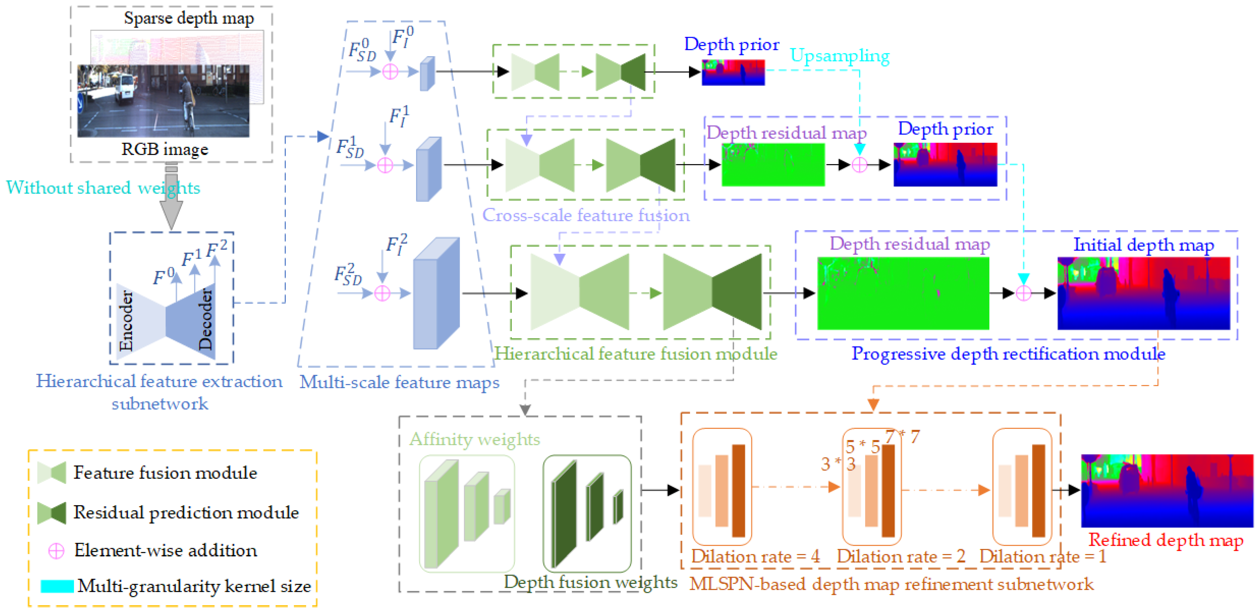
Figure 1. Overview of the proposed HFF-Net architecture, which includes the hierarchical feature extraction subnetwork, the hierarchical depth completion architecture that integrates the hierarchical feature fusion module and progressive depth rectification module, and the MLSPN-based depth map refinement subnetwork to achieve a state-of-the-art depth completion result.
Ijgi 14 00412 g001
Figure 2. The detailed structure for generating robust multi-scale feature maps.
Ijgi 14 00412 g002
Figure 3. Detailed structure of the hierarchical depth completion subnetwork.
Ijgi 14 00412 g003
Figure 4. Detailed process of the MLSPN-based depth map refinement subnetwork.
Ijgi 14 00412 g004
Figure 5. Overview of some representative scenes in both datasets. From top to bottom represent the RGB images, the sparse depth maps, and the ground-truth depth map of the KITTI DC and NYUv2 datasets.
Ijgi 14 00412 g005
Figure 6. Qualitative comparison of the predicted dense depth maps with those of some of the state-of-the-art methods on the KITTI DC test set. The second and last columns are the enlarged results of the yellow rectangular regions of the first and third columns, respectively. From top to bottom are the RGB images, sparse depth maps, and the predicted depth maps by CSPN++, GuideNet, PENet, CFormer, and HFF-Net, respectively.
Ijgi 14 00412 g006
Figure 7. Qualitative comparison of the predicted dense depth maps with those of some of the state-of-the-art methods on the NYUv2 test set. The second and last columns are the enlarged results of the blue rectangular regions of the first and third columns, respectively. From top to bottom, respectively, are the RGB images, sparse depth maps, ground-truth depth maps, and the predicted depth maps of NLSPN, CFormer, and HFF-Net.
Ijgi 14 00412 g007
Figure 8. Qualitative comparison of the predicted depth maps of the different model variants on the KITTI DC validation set. The second and last columns are enlarged parts of the black rectangular regions of the first and third columns, respectively. From top to bottom are the RGB images, sparse depth maps, and the predicted depth maps of Baseline, Model-Net1, Model-Net2, Model-Net3, Model-Net4, Model-Net5, and HFF-Net, respectively.
Ijgi 14 00412 g008
Figure 9. Qualitative comparison of the predicted depth maps for different-level sparsity measurements on the KITTI DC validation set. From left to right, respectively, are the results for the 4-line, 16-line, and 64-line scenarios. From top to bottom are the RGB images, the sparse depth maps, and the predicted depth maps of GuideNet, NLSPN, CFormer, LRRU, and HFF-Net, respectively.
Ijgi 14 00412 g009
Figure 10. Qualitative comparison of the predicted dense depth maps on the SUN RGB-D test set. From top to bottom, respectively, are the RGB images, input depth maps, ground-truth depth maps, and the predicted depth maps of NLSPN, CFormer, and HFF-Net.
Ijgi 14 00412 g010
Table 1. The detailed encoder–decoder architecture of the hierarchical feature extraction subnetwork.
InputSettingOutput
I or S D 3 × 3 × 32 H × W × 3 or H × W × 1
Conv0_1 3 × 3 × 64 H × W × 32
Conv0_2 3 × 3 × 64 3 × 3 × 64 × 2 , s = 2 H × W × 32
Conv1_1 3 × 3 × 64 3 × 3 × 64 × 2 , s = 2 H 2 × W 2 × 64
Conv2_1 3 × 3 × 64 3 × 3 × 64 × 2 , s = 2 H 4 × W 4 × 64
Conv3_1 3 × 3 × 64 3 × 3 × 64 × 2 , s = 2 H 8 × W 8 × 64
Conv4_1 3 × 3 × 64 3 × 3 × 64 × 2 , s = 2 H 16 × W 16 × 64
Conv5_1 3 × 3 × 64 3 × 3 × 64 × 2 , s = 2 H 32 × W 32 × 64
Dconv1_1Deconv 5 × 5 × 64 , s = 2
add Conv4_1
H 16 × W 16 × 64
Dconv2_1Deconv 5 × 5 × 64 , s = 2
add Conv4_1
H 8 × W 8 × 64
Dconv3_1Deconv 5 × 5 × 64 , s = 2
add Conv4_1
H 4 × W 4 × 6
Dconv4_1Deconv 5 × 5 × 64 , s = 2
add Conv4_1
H 2 × W 2 × 64
Dconv5_1Deconv 5 × 5 × 64 , s = 2
add Conv4_1
H × W × 64
Table 2. The datasets and implementation details used in the experiments.
DatasetsImage ResolutionData SplittingBatch SizeEpochs
KITTI DC1226 × 370 pixels85,898, 1000, and 1000 image frames were used for model training, validation, and testing, respectively.330
NYUv2640 × 480 pixels45,205, 2379, and 654 image frames were used for model training, validation, and testing, respectively.12100
Table 3. Quantitative evaluation results for the KITTI DC test set. The best and second-best results are marked in bold and underlined, respectively.
MethodsRMSE (mm) ↓MAE (mm) ↓iRMSE (1/km) ↓iMAE (1/km) ↓
CSPN [26]1019.64279.462.931.15
SD2 [55]814.73249.952.801.21
GAENet [70]773.90231.292.291.08
DeepLiDAR [71]758.38226.502.561.15
ACMNet [52]744.91206.092.080.90
CSPN++ [24]743.69209.282.070.90
NLSPN [21]741.68199.591.990.84
GuideNet [56]736.24218.832.250.99
PENet [22]730.08210.552.170.94
GuideFormer [45]721.48207.762.140.97
CFormer [17]708.87203.452.010.88
LRRU [1]696.51189.961.870.81
HFF-Net694.90201.541.950.88
Table 4. Quantitative evaluation results for the NYUv2 test set. The best and second-best results are marked in bold and underlined, respectively.
MethodsRMSE (m) ↓REL ↓ σ 1.25  (%) ↑ δ 1.25 2  (%) ↑ δ 1.25 3 (%) ↑
SD2 [55]0.2300.04497.199.499.8
CSPN [26]0.1170.01699.299.9100.0
CSPN++ [24]0.116----
DeepLiDAR [71]0.1150.02299.399.9100.0
ACMNet [52]0.1050.01599.499.9100.0
GuideNet [56]0.1010.01599.599.9100.0
NLSPN [21]0.0920.01299.699.9100.0
LRRU [1]0.0910.01199.699.9100.0
CFormer [17]0.0900.01299.699.9100.0
HFF-Net0.0930.01399.699.9100.0
Table 5. Quantitative evaluation results for the KITTI DC validation set. The best and second-best results are marked in bold and underlined, respectively.
ModelsHierarchical Depth Completion SubnetworkMLSPN-Based Depth Refinement SubnetworkResults (mm)
Full-Scale1/2-Scale1/4-Scale1/8-Scale D R 1 D R 2 D R 3 RMSE ↓MAE ↓
Baseline 754.60220.42
Model-Net1 746.89231.74
Model-Net2 739.72225.44
Model-Net3 747.03240.62
Model-Net4 733.05206.91
Model-Net5 732.05205.83
HFF-Net 726.21200.64
Table 6. Quantitative evaluation results for the KITTI DC validation set with different-level sparse depth measurements. The best and second-best results are marked in bold and underlined, respectively.
MethodsScanning LinesRMSE (mm) ↓MAE (mm) ↓
GuideNet [56]1-line20,432.8714,620.19
NLSPN [21]1-line14,005.349086.54
CFormer [17]1-line16,079.9911,719.06
LRRU [1]1-line15,513.8311,282.55
HFF-Net1-line13,985.019079.81
GuideNet [56]4-line15,259.4610,224.12
NLSPN [21]4-line6154.773416.86
CFormer [17]4-line6907.374080.68
LRRU [1]4-line7628.764204.29
HFF-Net4-line6709.293847.34
GuideNet [56]8-line7102.854548.64
NLSPN [21]8-line3722.921697.49
CFormer [17]8-line3639.231749.24
LRRU [1]8-line3610.211588.76
HFF-Net8-line3495.121730.93
GuideNet [56]16-line3122.791292.43
NLSPN [21]16-line1974.55672.50
CFormer [17]16-line2178.57752.09
LRRU [1]16-line1883.25676.93
HFF-Net16-line1835.00654.21
GuideNet [56]32-line1385.81475.08
NLSPN [21]32-line1192.62347.92
CFormer [17]32-line1380.82400.03
LRRU [1]32-line1125.11353.77
HFF-Net32-line1129.75358.89
GuideNet [56]64-line760.19218.90
NLSPN [21]64-line790.67201.28
CFormer [17]64-line821.74211.38
LRRU [1]64-line743.04196.18
HFF-Net64-line726.21200.64
Table 7. Comparison of the model’s generalization performance for the SUN RGB-D test set. The best and second-best results are marked in bold and underlined, respectively.
MethodsParams (M)Memory (GB)RMSE (m) ↓REL ↓Time (s)
NLSPN [21]26.230.902.2691.1210.279
CFormer [17]83.514.770.5580.1500.154
HFF-Net8.957.080.4900.1090.168
Disclaimer/Publisher’s Note: The statements, opinions and data contained in all publications are solely those of the individual author(s) and contributor(s) and not of MDPI and/or the editor(s). MDPI and/or the editor(s) disclaim responsibility for any injury to people or property resulting from any ideas, methods, instructions or products referred to in the content.