Article

Numerical Assessment of a High-Level Rock Failure Potential Based on a Three-Dimensional Discrete Element Model

1
Key Laboratory of Geological Hazards Mitigation for Mountainous Highway and Waterway, Chongqing Municipal Education Commission, Chongqing Jiaotong University, Chongqing 400074, China
2
Key Laboratory of Construction and Safety of Water Engineering of the Ministry of Water Resources, China Institute of Water Resources and Hydropower Research, Beijing 100038, China
3
Institute of Mountain Hazards and Environment, Chinese Academy of Sciences, Chengdu 610041, China
4
SHAANXI LIZHENG Investigation and Design Co., Ltd., Xi’an 710000, China
*
Author to whom correspondence should be addressed.
ISPRS Int. J. Geo-Inf. 2025, 14(10), 402; https://doi.org/10.3390/ijgi14100402
Submission received: 15 July 2025 / Revised: 8 October 2025 / Accepted: 10 October 2025 / Published: 15 October 2025

Abstract

The estimation of the area susceptible to rock failure and the prediction of its movement process are pivotal for hazard mitigation, yet they are also challenging. In this study, we proposed a novel integrated method combining field investigation, remote sensing, and three-dimensional discrete element method (DEM) simulation to achieve our goal. The field investigation and remote sensing analysis are used for the purpose of ascertaining the deformation phenomenon and the structure of the rock slope, identifying the potential failure position and area of the slope. Subsequently, a three-dimensional DEM simulation is employed to quantitatively assess the potential rock failure-affected area and movement process, based on the above potential failure information. The simulation results demonstrate that potential rock failure persists for approximately 30 s, and its movement process can be categorized into two distinct stages: acceleration and deceleration. The initial acceleration stage is characterized by a duration of 10 s, culminating in a peak average velocity of 13 m/s. The subsequent deceleration stage extends for a duration of 20 s. Notably, the maximum attainable velocity for the segment of rock mass under consideration is estimated to be 50 m/s. Furthermore, the model demonstrates the variation in fracture energy, friction energy, and kinetic energy over time. The potential affected area is 140,000 m2, and approximately 8000 m2 of residential construction will be destroyed if a rock failure occurs. It is imperative to implement measures aimed at the prevention of rock failure in order to mitigate the risk of such an occurrence.

1. Introduction

Rock failure is a critical geological disaster with global implications, frequently endangering infrastructure and public safety [1]. The precarious nature of many slopes, existing in a metastable state, renders them susceptible to rock failure occurrences triggered by various factors such as heavy rainfall and seismic activity [2]. The accurate forecasting of potential rock failure-affected areas is paramount for the implementation of effective risk mitigation strategies. However, quantitative forecasting for rock failure-affected areas and its dynamic analysis of movement is still difficult and challenging [3,4].
Previous research about affected areas of rock failure forecasting focuses on its stability analysis before failure. Based on the material and structure information of the rock slope, the factor of safety (FOS), which assesses the currant stability status of slopes, can be acquired [5,6]. However, the post-failure movement process cannot be acquired from the stability analysis. Forecasting the extent of slope failures requires analyzing post-failure movement processes. However, the limit equilibrium method cannot analyze deformation issues due to its static nature, and conventional finite element methods struggle to analyze block detachment and violent impact processes due to mesh limitations [3,5,6]. The limitation makes it difficult to forecast post-failure behavior and dynamic movement of potential rock failure. In recent years, significant progress has been made in the field of rock failure post-failure behavior through the introduction of advanced computational techniques. Numerical methods including continuum methods and discontinuum methods have been applied for landslide movement assessment. Continuum methods such as the Smoothed Particle Hydrodynamics (SPH) [7,8], the Material Point Method (MPM) [9,10], and Computational Fluid Dynamics (CFD) [11,12] for landslide simulation treat the slope material as the continuum medium. They solve the conservation equations of continuum mechanics while naturally handling extreme distortions, free surfaces, and material separation without mesh entanglement. They excel at simulating the entire landslide process—from initial failure to post-failure runout—capturing soil/rock behavior as it transitions from solid to fluid-like flow. These continuum methods have emerged as powerful tools for simulating rock failure events with enhanced accuracy and detail [13,14,15,16,17,18]. Discontinuum methods like the Discrete Element Method (DEM) [19,20,21] and Discontinuous Deformation Analysis (DDA) [22,23,24] explicitly model landslides as assemblies of distinct blocks or particles. They track granular materials through collisions and contact forces, capturing flow dynamics and deposition. Moreover, discontinuum methods have gained prominence for their ability to capture the intricate interactions within rock masses, particularly in scenarios involving large deformations [19,20,21,22,23,24]. Quantitative information such as mass movement distance, speed, and geometry of the rock failure can be acquired from the above numerical methods, making rock failure scale prediction possible.
In this study, we proposed an integrated approach to predicting the area potentially affected by rock failure, combining field investigations and DEM simulations based on a relatively novel Rigid Block (RBlock) model [25]. The Rblock model is a discrete element method in which discrete elements are represented by polyhedral rigid bodies. Compared to traditional discrete element models of particle flow based on spherical particles, the Rblock model is more effective in characterizing the polyhedral rock blocks generated by rock fragments. A metastable rock slope in Guizhou province was studied. To know the potential affected area of the rock failure, a field investigation was carried out first to determine the potential failure position and rock mass. Then, a model based on blocky DEM was used for assessment based on the field investigation. Information about potential post-failure behavior and affected area was acquired quantitively from the simulation, which can be used for disaster prevention and mitigation.

2. Background

2.1. Study Area

The location of the rock slope is Zhongzhai town, Zhijin county, Bijie City, Guizhou province. The study area is located in the west of the Guizhou Plateau (Figure 1). The geographical area under consideration is a low-to-medium plateau landform, characterized by substantial undulating terrain and a terrain slope of 15~85°. The geographical area under consideration is characterized by a subtropical monsoon climate. The region’s climate is characterized by mild and humid conditions, with precipitation being concentrated from April to October, resulting in an annual rainfall total of 1479.3 mm.

2.2. Geological and Topographical Condition

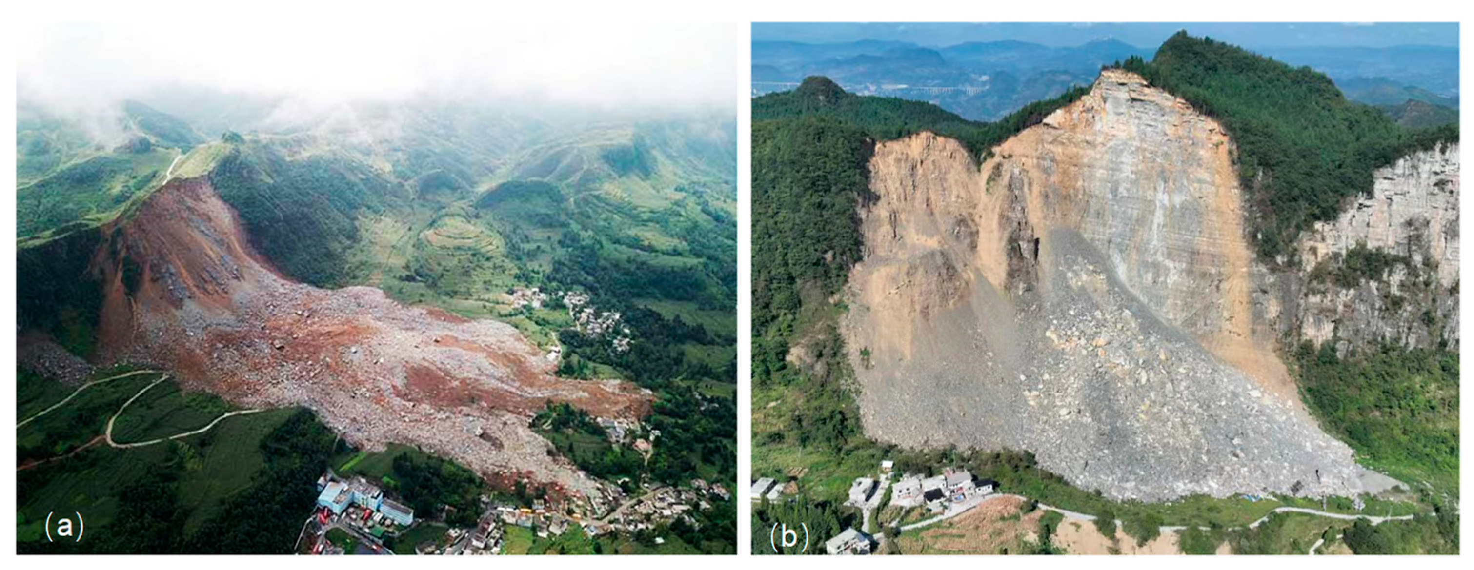
The geographical area under consideration is part of the Yangtze Para platform. The lithology of the study area is principally composed of quaternary deposits, mudstone, sandstone, and limestone. The presence of active tectonic movements gives rise to a complex geological environment characterized by numerous faults [26]. The direction of these faults is predominantly north-easterly, a phenomenon attributable to tectonic movements. These faults have been observed to play a pivotal role in the magnitude of geological disasters, including landslides and rockfalls. It is evident that the region is subject to frequent tectonic movements and a variety of lithological compositions, resulting in a prevalence of fragmental rock formations. These rocks exhibit a comparatively low level of strength, characterized by a high incidence of fractures. It is evident that rockfalls are a frequent occurrence in the study area, particularly in Bijie City. For instance, two substantial rockslides transpired on 28 August 2017 and 30 May 2024, correspondingly (Figure 2) [27,28,29,30]. The two rockslides resulted in significant financial loss, with the former even traversing 800 m along the runout path [30]. Moreover, two rock avalanches occurred in 2020 and 2022 in the coal mining area of Zhijin County, which also exhibited long-runout characteristics [31]. Consequently, the estimation of the potential magnitude of rock failure in this region is imperative.

2.3. Deformation Phenomenon

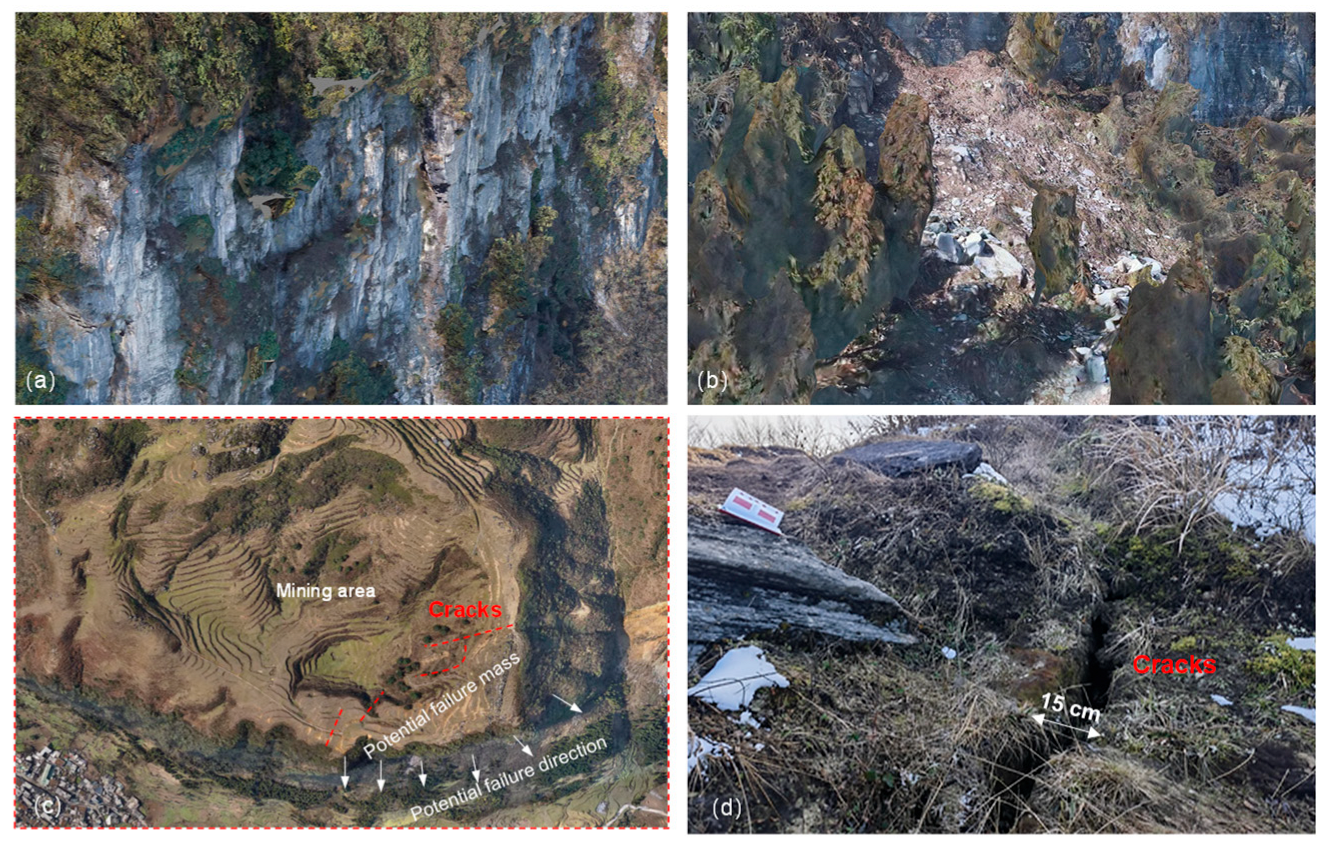
The metastable rock slope is located in a coal mine area. The incline of the rock is precipitous, with a dip angle ranging from 68 to 88° and an incline direction of 93°. The incline of the slope ranges from 110 to 140 m. Due to excavation, some rock masses have undergone unloading and relaxation, resulting in reduced rock strength. The presence of three distinct groups of joints within the rock formation is evident, delineating a blocky structural configuration (Figure 3a). The external loads to which the rock slope is subjected have resulted in its transformation into a potentially hazardous rock mass. As illustrated in Figure 3b, due to the unloading deformation toward the steep overhanging face of the original terrain, a significant number of metastable rock blocks have been dislodged from the slope, resulting in its collapse. With the exception of the collapsed rocks, a significant number of cracks have been identified along the edge of the slope. Some cracks are characterized by their considerable length and depth and are observed to be almost parallel to the edges of the slope (Figure 3c). The maximum aperture of the cracks was measured to be 0.15 m, with a maximum visible depth of 4 m (Figure 3d). Furthermore, the fractured surfaces of these cracks are curved and rough, indicating that they are tensile cracks. The formation of large-scale parallel tensile cracks in the crown, with a high degree of concentration, has been identified as a potential indicator of slope metastability [32,33,34,35]. This phenomenon suggests the possibility of large-scale rock failure. It is imperative to assess the potential failure scale of rock failure in the area at the toe of the slope, where a village and numerous houses are located.

3. Methodology

3.1. Discrete Element Method

The DEM based on PFC3D software was used to predict the potential rock failure. PFC3D (Particle Flow Code in 3 Dimensions) is a professional numerical simulation software based on the DEM for three-dimensional particle flow. It accurately simulates the entire dynamic process of rockfall hazards, from initiation, collision, and fragmentation to accumulation, by constructing assemblies of rock particles and joint networks, providing a critical numerical analysis tool for revealing disaster mechanisms and conducting risk assessments. As a quantitative analysis method, the DEM has been widely used and validated in the dynamic analysis of geological hazards such as landslides, debris flows, and rock failure [19,20,21,25]. As a quantitative analysis method, the DEM is a numerical method to study the mechanical behavior of discontinuous media. This study employs a RBlock model based on the DEM for numerical simulation [25]. This model discretizes the object of study (e.g., rock mass, masonry structure) into a series of rigid polyhedral elements that can move freely and interact with each other through contacts. The macroscopic mechanical behavior of the system is not manifested through the deformation of the elements themselves but is governed by the relative movements (including sliding, rotation, and opening) of these rigid elements at their contact points. This section will elaborate on the fundamental theory, contact relationships, governing equations, numerical solution scheme, and energy calculation principles of this model.
The RBlock model is founded on the following two core assumptions:
  • Rigid Block Assumption: Each discrete element (block) is treated as an absolutely rigid body, meaning it itself undergoes no elastic or plastic deformation. All system strain energy is stored at the contacts between blocks.
  • Finite Displacement and Rotation Assumption: Blocks can undergo arbitrarily large displacements and rotations during loading, making this model particularly suitable for simulating highly nonlinear mechanical processes such as large deformation, disintegration, and collapse.
The solution of the model is based on the Explicit Dynamic Relaxation Method, which tracks the dynamic evolution of the entire system by directly integrating the equations of motion.
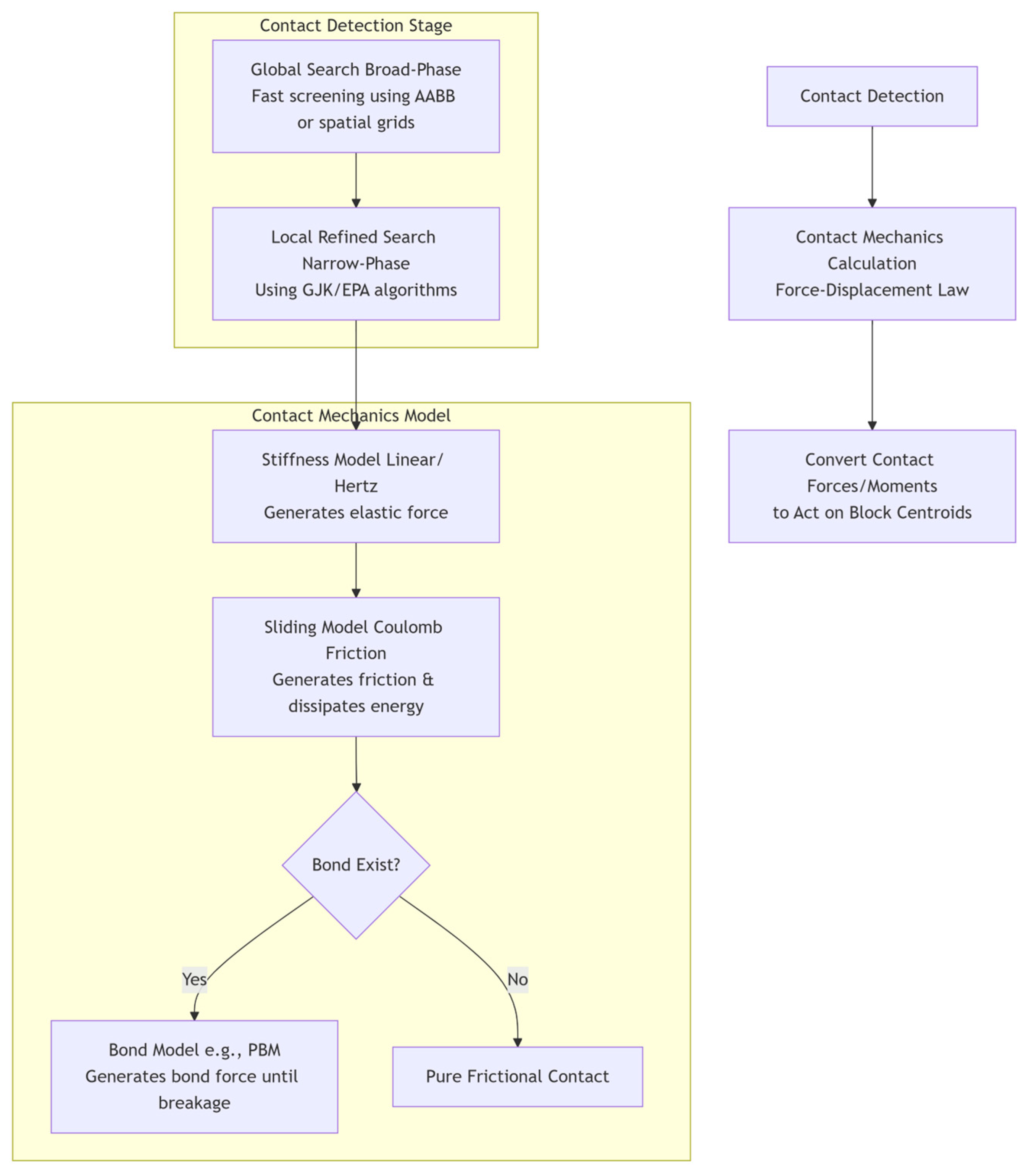
The treatment of contact relationships between blocks is the core of the calculation. The process is iterative, as shown in Figure 4, and consists of two main stages: contact detection and contact mechanical response.
The contact detection algorithm in discrete element methods, particularly for RBlock models, is a sophisticated two-tiered process designed to efficiently and accurately identify interactions between geometrically complex bodies within a computationally feasible framework. It addresses the prohibitive quadratic complexity of checking all possible pairs by first employing a broad-phase search, which utilizes spatial partitioning strategies like axis-aligned bounding boxes (AABB), spatial grids, or the sweep and prune algorithm to rapidly eliminate pairs of blocks that are clearly far apart, generating a manageable shortlist of potential contacts. This list is then processed by a narrow-phase search, centered on the Gilbert–Johnson–Keerthi (GJK) algorithm, which leverages the concept of the Minkowski difference to determine whether two convex bodies intersect by iteratively constructing a simplex and checking for the inclusion of the origin. For intersecting pairs, the Expanding Polytope Algorithm (EPA) is invoked to precisely calculate the penetration depth and contact normal by expanding the final simplex from GJK into a convex polytope and iteratively refining the closest face to the origin. This elegant combination of strategies transforms an intractable computational problem into an efficient one, ensuring that detailed geometric information—essential for applying force-displacement laws at contacts—is determined only for interacting pairs, thereby forming the critical foundation for the dynamic simulation of blocky systems.
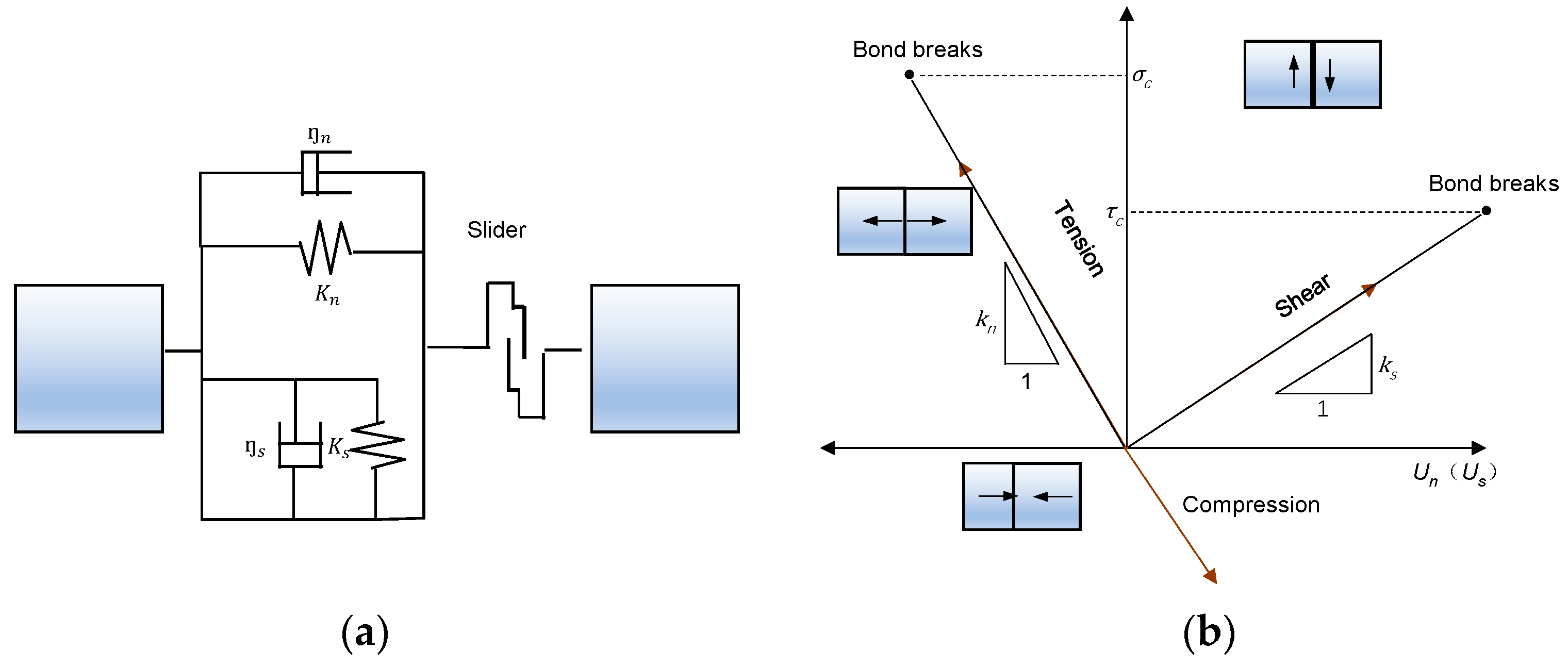
Once contact is detected, the contact force is calculated based on the overlap and relative displacement (Figure 5). The displacement and force of the blocky elements follow the force-displacement contact law and Newton’s second law. The contact force between individual dissenting elements is divided into radial force and tangential force; the magnitude of these two forces is determined by element contact stiffness and the friction coefficient. The radial force and tangential force can be calculated as follows:
F n = K n δ n
F s = m i n K s δ s , μ F n
where Kn and Ks are normal and tangential stiffness coefficients, respectively, δn and δs are normal and tangential overlap, respectively, and μ is the friction coefficient.
A parallel bonding model (PBM) is used to describe the cohesion property between rock blocks because it has been most widely used for rock avalanche simulation [4,36]. PBM provides the mechanical behavior of a cement-like material between two contact blocks. PBM acts in parallel with linear members and establishes elastic interactions between members. The existence of PBM can also simulate slip behavior. PBM can transfer forces and moments between contact blocks. PBM can be thought of as a group of elastic springs with steady normal and shear stiffness, evenly spread across a cross-section on the contact plane. The springs operate in conjunction with the springs of the linear component. After forming the parallel bond, the relative motion at the contact point induces a force and moment in the bonded material. The force and moment exerted on the two contact blocks are connected to the peak normal and shear stresses in the bonding material surrounding the bond. If any of these maximum stresses exceed their corresponding bond strength (Equations (3) and (4)), the parallel bond fractures and the bond material are removed from the model along with the accompanying forces, moments, and stiffness.
σ = F n A + | M | R I σ c
τ = F s A + | T | R J τ c
where A , I , and J are the bond’s area, moment of inertia, and polar moment of inertia, respectively; σ and τ are the bond’s tensile and shear strengths, respectively; and R is the bond radius. Violation of either criterion causes the bond to break, and the contact thereafter reverts to a pure frictional contact.
In each step of computation, the resultant force and bending moment of each element are calculated according to the amount of overlap between elements. Then, the displacement and velocity of the elements in the iteration time step are calculated by combining their velocity and the angular velocity according to the mechanical characteristics of the elements as the following equations. The spatial position of the elements is also calculated after this time step:
m d v d t =   F e x t
where m is the mass, v is the velocity, and F e x t is the resultant external force.
I d ω d t =   M e x t
where I is the inertia tensor, ω is the angular velocity, and M e x t is the external torque.
The Central Difference Method (Velocity-Verlet algorithm) is used for explicit integration of the equations of motion:
v t + Δ t 2 = v ( t ) + a ( t ) Δ t 2
x ( t + Δ t ) = x ( t ) + v t + Δ t 2 Δ t
where x , v , and a are the displacement vector, velocity vector, and accelerate vector, respectively.
In RBlock simulations based on the DEM, energy calculation is not a mere post-processing tool but a core component for understanding the system’s mechanical behavior, verifying the physical correctness of the simulation, and quantifying energy transformation and dissipation mechanisms. This framework strictly adheres to the First Law of Thermodynamics, i.e., the principle of energy conservation.
The total energy of the system primarily consists of three major components: kinetic energy, strain energy, and dissipated energy. Kinetic energy ( E k ) characterizes the macroscopic motion state of the system and is the sum of the translational and rotational kinetic energy of all blocks. It is calculated as follows:
E k = i = 1 N 1 2 m ( i ) v ( i ) 2 + 1 2 ω ( i ) I ( i ) ω ( i )
where m ( i ) , v ( i ) , I ( i ) , and ω ( i ) represent the mass, translational velocity, inertia tensor, and angular velocity of block i, respectively. Its rate of change directly reflects the power input by the resultant external forces.
Strain energy ( E e ) represents the elastic potential energy stored within the system, primarily distributed in the elastic springs at contacts between blocks. It is precisely calculated based on the quadratic relationship between contact force and the corresponding displacement:
E e = j = 1 M 1 2 F n ( j ) 2 K n ( j ) + 1 2 F s ( j ) 2 K s ( j )
Here, F n ( j ) and F s ( j ) are the normal and tangential forces at contact j, and K n ( j ) and K s ( j ) are the corresponding contact stiffness values. For the Parallel Bond Model (PBM), this formula must be extended to include the bending strain energy generated by moments and torques.
Energy dissipation occurs primarily through two irreversible physical processes. Frictional energy ( E f ) is calculated using the Coulomb friction model. It represents the work performed by the tangential force over the relative sliding displacement at a contact, which is irreversibly converted into heat and dissipated from the system. Its increment is calculated by the following:
Δ E f =   F s Δ δ s
Bond breakage energy ( E b ) is the instantaneous release of the elastic strain energy stored within a parallel bond when it undergoes brittle failure upon reaching its strength limit. Furthermore, a small amount of global damping is often introduced to allow the system to dynamically relax to a state of static equilibrium, and the kinetic energy dissipated by this damping also contributes to the total energy balance.

3.2. Numerical Model Construction and Setting

In order to undertake the numerical simulation, it is first necessary to create a three-dimensional terrain model. The construction of the three-dimensional terrain model is predicated on a digital terrain model (DTM) data set with a high resolution of 5 m. The acquisition of cloud point data of the DTM is facilitated by ArcGIS software and, subsequently, a three-dimensional computer-aided design (CAD) software is employed to construct the three-dimensional model. In the numerical model under consideration, the metastable rock is represented by blocky elements, while the slip surface is represented by wall elements. The number of block elements is set at 11,258, with the objective of optimizing both computational efficiency and accuracy (Figure 6).
The composition of the block elements of the source rock and ground surface was defined as rock material. The physical, mechanical, and numerical parameters employed in the simulation are obtained according to the lithologic materials and physical tests. It is evident that the numerical model parameters and dynamic parameters are influenced by the severe weathering of the perilous rock belt. This has resulted in the development of joint fractures, which are characterized by a high degree of fragmentation. In this study, a number of rock landslides and rock avalanches in Bijie City were examined, and it was found that the bonding parameters taken by the numerical simulation of rock mass were low. The following section will provide a comprehensive overview of the relevant literature on the subject. Due to the similarity of the ground conditions, the coefficient of friction between the failure body and the ground is referred to as the Nayong rock avalanche and other similar rock avalanche in Guizhou province [26,27,28,29,30,37,38,39], and the parameters used in the simulation are shown in the table below (Table 1).

4. Numerical Simulation Results

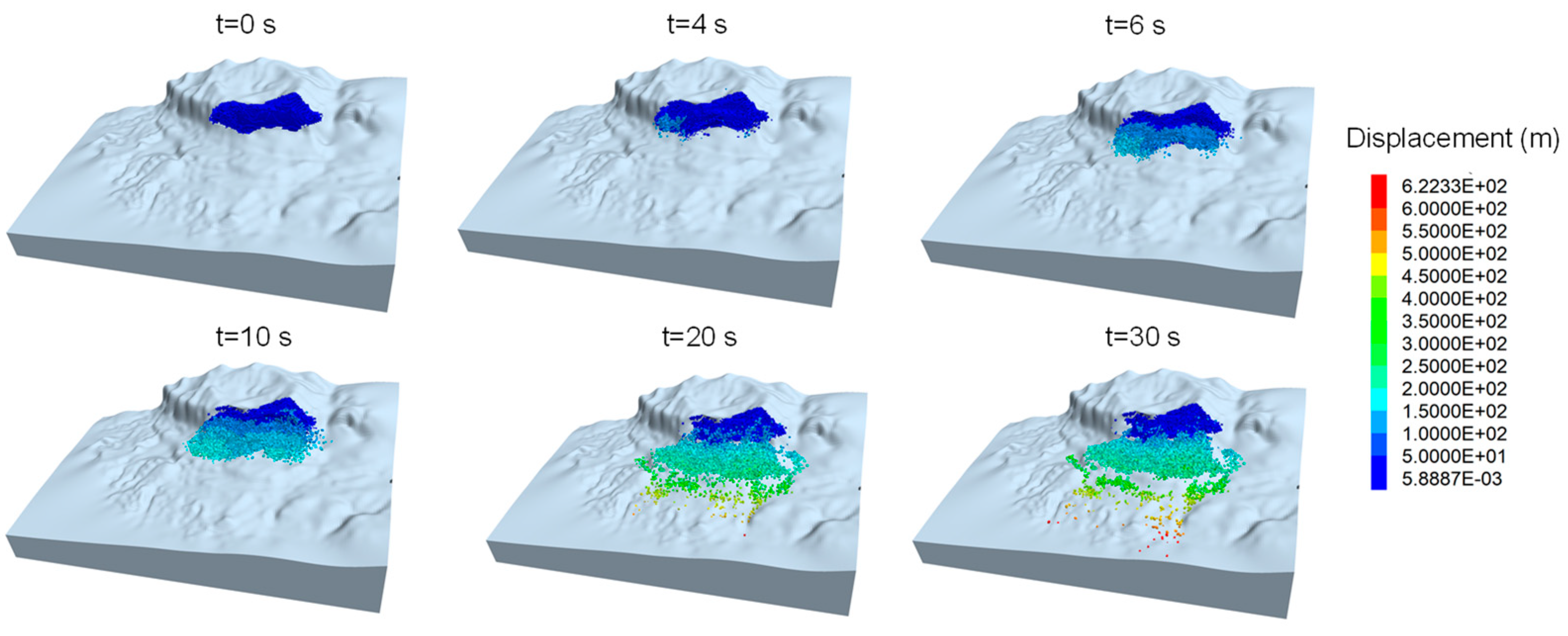
According to the simulation results, the entire process of rock failure is about 30 s (Figure 7). After rock failure starts, the deformation of potential rock mass is slow in the first 4 s, and the displacement of rock mass is approximately zero. Only a few small rocks fall and move. At 6 s, the left part of the rock mass starts to deform obviously with the maximum displacement of 50 m. After this time, the rock mass gradually presents a large scale of collapse. At 10 s, the front part of the movement mass reaches the bottom of the slope and moves some distance with the maximum distance of 200 m. At 20 s, most of the movement mass stops moving and the maximum runout distance reaches 500 m. At 30 s, the movement mass completely stops moving. The failure part is mostly the front part of the movement mass, and some of the back part still remains stable. The front part moves a distance from 100 m to 400 m in general. Some blocks can reach a distance of 600 m.
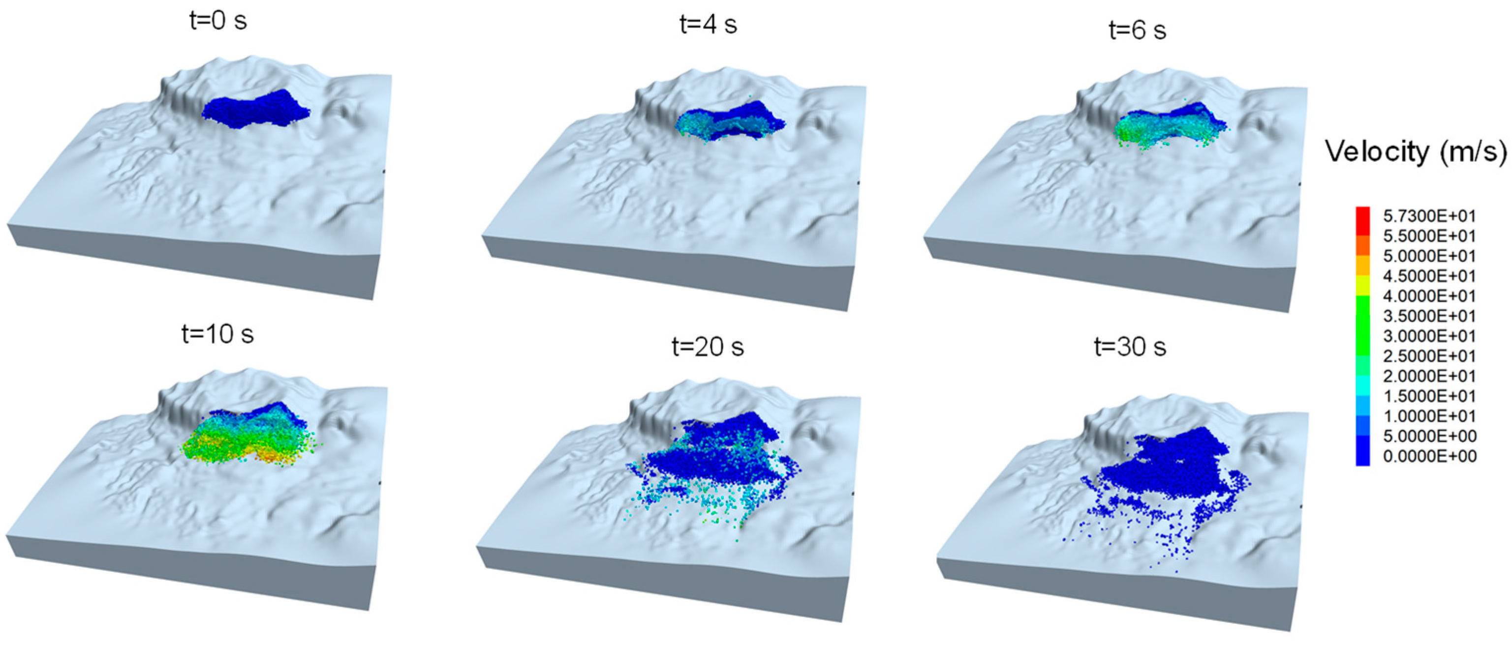
Except for mass movement displacement, movement speed of the movement mass at different times can also be acquired from the simulation (Figure 8). It can be found out that the left and middle part of the source rock starts to move first at 4 s, and then it drives the source rock of the entire middle part to start moving at 6 s. Movement of the source rock develops rapidly, and a large scale of source rock rapidly moves. The maximum speed of partial rock mass can reach 50 m/s at 10 s. After falling down to the bottom surface, the movement mass starts to decelerate because of collision and friction. At 20 s, the major part of the movement mass stops moving, and only some rock blocks still move with a velocity from 0 to 15 m/s. At 30 s, the movement mass completely stops moving and almost all the blocks have a velocity of 0.
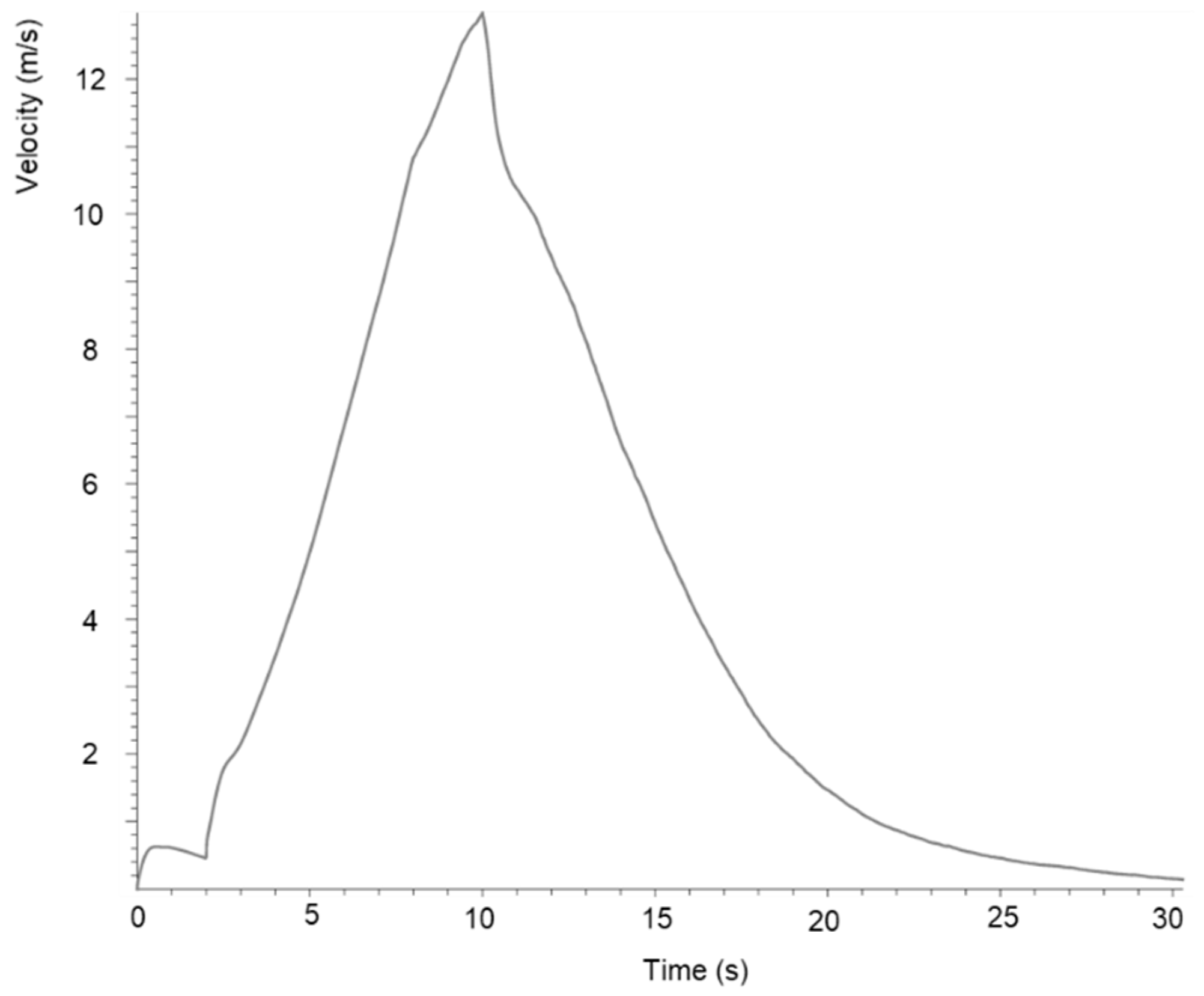
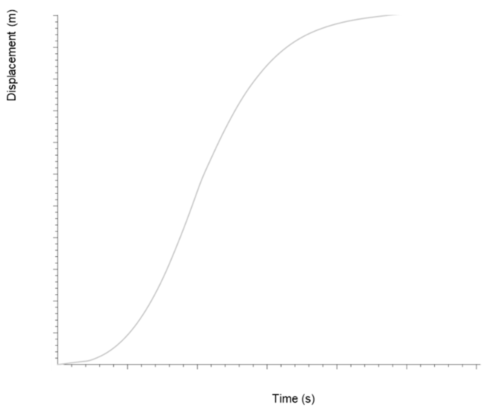
To further quantitatively realize the movement characteristics of the source rock, the variation in average speed (Figure 9) and displacement (Figure 10) of the movement mass with time are recorded. It can be found out that the mass movement can be divided into two stages in general: acceleration stage and deceleration stage. After slope failure, the movement mass constantly accelerates under gravity. At 10 s, the movement mass reaches the peak average speed of 13 m/s, and then it constantly decelerates due to collision and friction between bottom terrain. From 10 s to 20 s, the mass constantly falls down, and collision plays a dominant role in deceleration, so the speed of the movement mass decreases rapidly. After 20 s, almost all of the movement mass reaches the bottom surface, and friction plays the dominant role in deceleration. At this period, its deceleration tendency obviously becomes slower compared to the collision stage.
Except for the above dynamic parameters, variation in energy such as kinetic energy, fracture energy, and friction energy of the movement mass can also be acquired from the model.
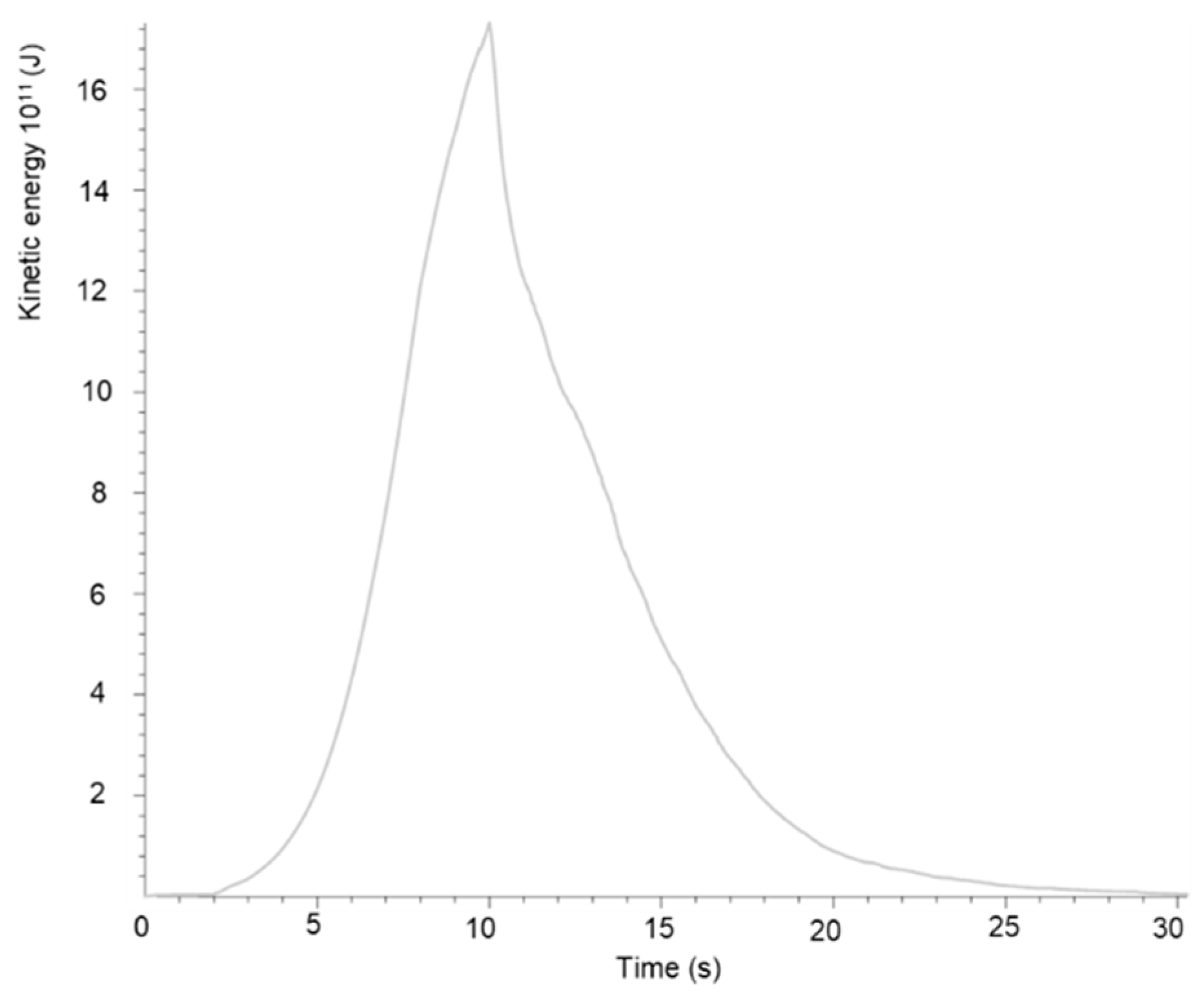
As illustrated in Figure 11, the variation in kinetic energy of the movement mass with time is demonstrated. It has been determined that the movement mass can be divided into two movement stages, as evidenced by the variation in movement speed. Subsequent to slope failure, the source rock will begin to move and fall downwards under the force of gravity. Concurrently, the gravitational potential energy of the slide will be continuously converted into kinetic energy. Subsequently, the movement mass arrives at the base of the slope, where it collides with the ground surface and experiences a rapid deceleration, resulting in a sudden and significant decrease in kinetic energy at 10 s. Following this, within 20 s, the majority of the movement mass has attained the bottom surface, leading to a gradual decline in kinetic energy due to the friction generated by the moving block.
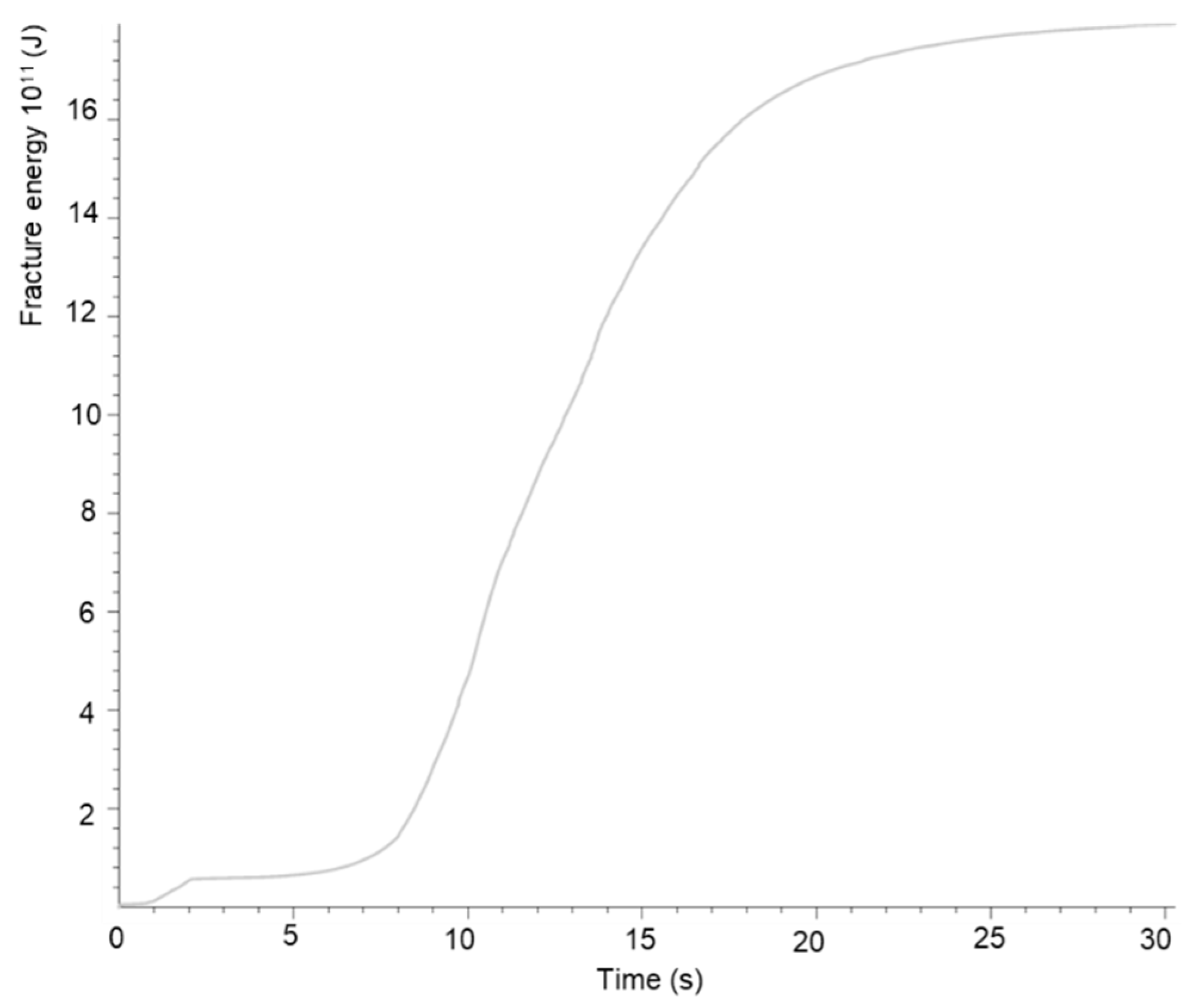
Figure 12 shows the variation in fracture energy of the movement mass with time. It can be found out that the increase in fracture behavior is slow before 7 s. At this stage, only the left part of the rock mass fractures and moves from Figure 7. After 7 s, large-scale rocks fracture and collapse due to the change in stress state from the detachment of rock mass, and then the fracture energy suddenly increases rapidly. Due to the large-scale rock mass movement and dynamic fragmentation, the fracture energy continues to increase rapidly for a period of time. After 20 s, most of the movement mass stops moving, making the dynamic fragmentation behavior suddenly decline. This leads to the slow increase in fracture energy.
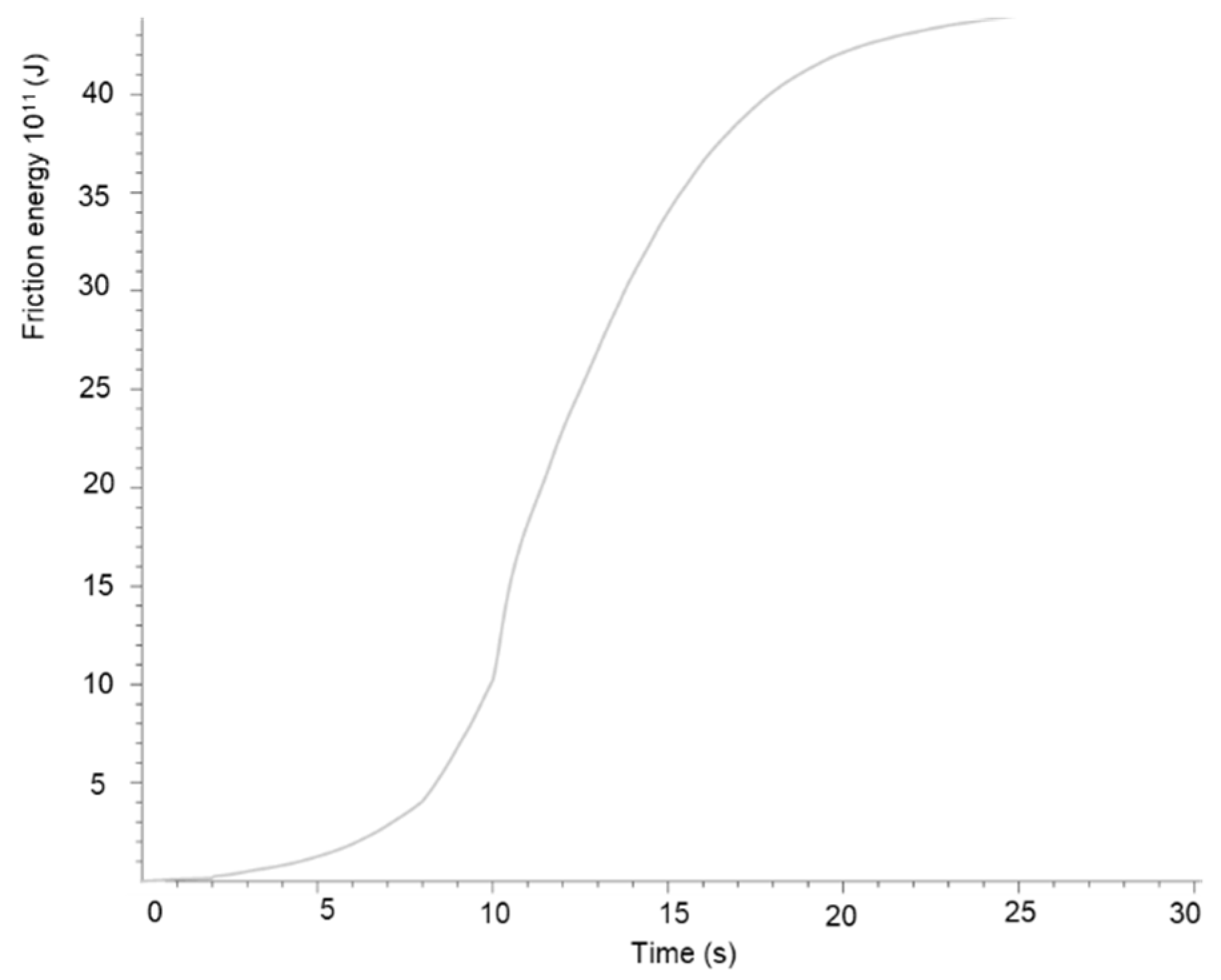
Figure 13 shows the friction energy of the movement mass with time. It can be found out that the friction energy generally increases in the whole movement stage, and it can be divided into three stages according to the growth rate. The first stage is from 0 to 10 s; the friction energy is generally small, but its growth rate constantly increases. This is because mass movement gradually becomes intense with time, and relative displacement increases at that stage. Greater relative displacement can make friction force perform more tapping. From 10 s to 20 s, the growth rate of friction energy is rapid, and this is because the mass movement is very intense in this stage. Both the relative displacement between movement mass and slip surface as well as movement mass are great, therefore making friction energy increase rapidly at that stage. After 20 s, although the friction energy still increases, the growth rate becomes smaller and smaller. At this stage, the mass movement gradually stops, making relative displacement gradually become smaller.
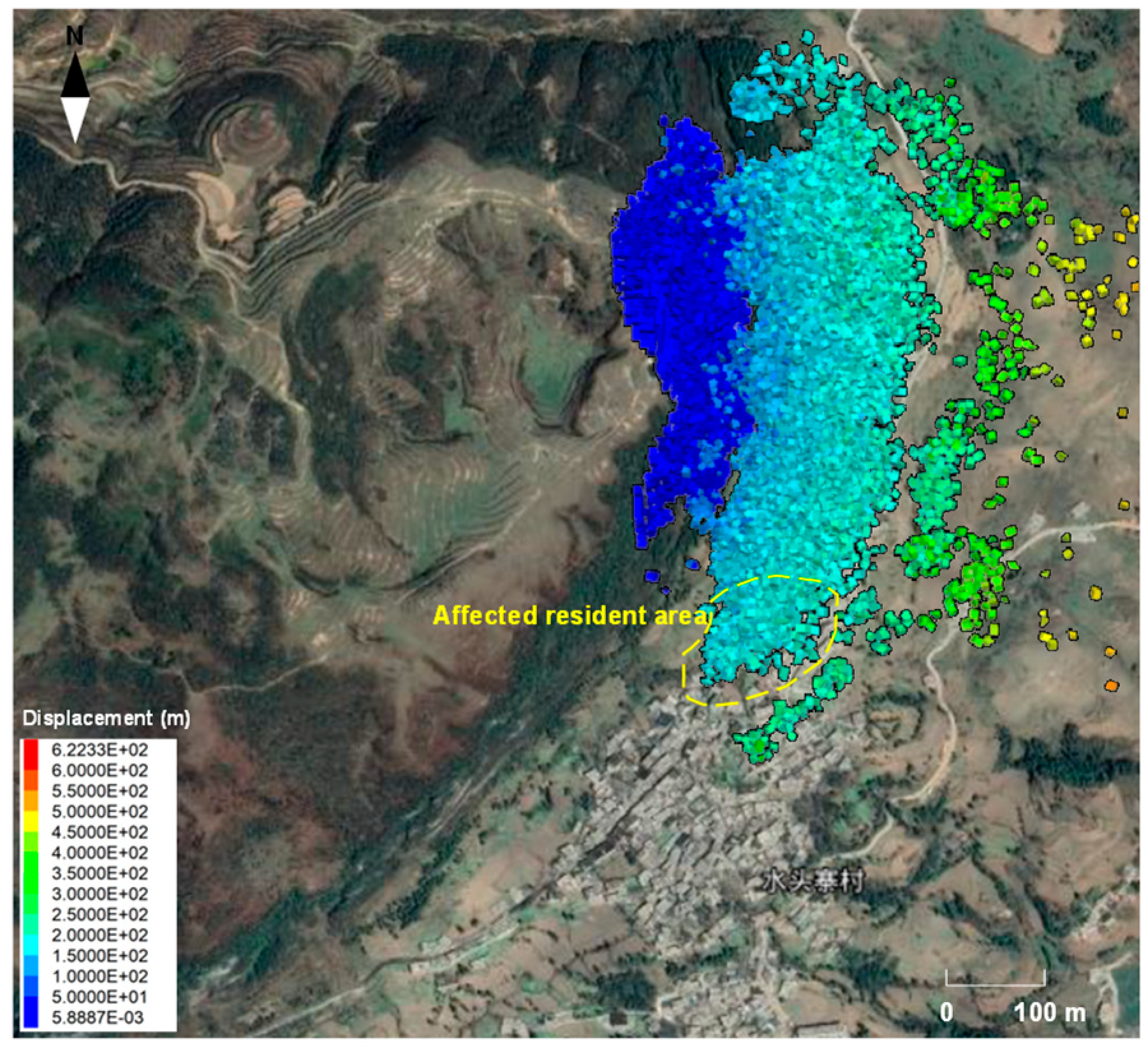
The simulation results above show that the average velocity and kinetic energy of the sliding mass first increase and then decrease in general, which is consistent with the observed parameter evolution patterns in simulations of the Baige rockslide [40,41], Xinmo rockslide [42,43], and Jichang rockslide [44,45] using other methods. The simulation results can be used to quantitatively judge whether the potential rock failure affects resident buildings. From the simulation results, the affected area of collapsed rocks is about 140,000 m2, and about 8000 m2 resident buildings will be destroyed by rock failure (Figure 14). This means that once rock failure occurs, it will cause a great loss. In the context of landslide disasters, distinct precursors have been observed to precede the occurrence of such events. These precursors include large-scale back-edge tensile cracks and differential settlement.

5. Conclusions

In this paper, we combined field investigation with DEM simulation in order to quantitatively predict the potential scale of rock failure, which has the potential to threaten a village. Field investigation is instrumental in determining the potential failure scale based on the deformation characteristics, including position of large-scale tensile cracks and settlement. These phenomena would provide key information on the potential location and volume of failure masses for post-failure analysis. In contrast, the DEM simulation based on the Rblock model is used to ascertain the post-failure process. The Rblock model uses polyhedral elements to represent rock blocks, and the simulation results show the model can adequately reflect rock failure movement and variation in key movement parameters. The DEM simulation indicates that the potential rock failure will last for approximately 30 s. The maximum distance traversed by the failed rock is estimated to be 500 m, with a maximum movement speed of 50 m per second. In addition to the aforementioned dynamic parameters, the model can also be used to calculate variations in kinetic energy, friction energy, and fracture energy. According to the findings of the simulation, in the event of a rock failure, 8000 m2 of residential constructions would be destroyed. This study demonstrates the applicability of the combined methods in rock failure prediction. Engineers can use the approach to determine whether protective measures are necessary, and it can also be used to assess the effectiveness of the protective measures and the potential disaster area after they have been implemented.

Author Contributions

Conceptualization, Yiding Bao; methodology, Xin Zhou and Yiding Bao; software, Xin Zhou; resources, Weifeng Zhang and Renzhe Zeng; original draft preparation, Xin Zhou and Yiding Bao; writing—review and editing. Xin Zhou, Yiding Bao, Weifeng Zhang and Renzhe Zeng; funding acquisition, Yiding Bao, Xin Zhou and Weifeng Zhang. All authors have read and agreed to the published version of the manuscript.

Funding

This work was supported by the National Natural Science Foundation of China (Grant No. 42571098,42207229), the Science Technology Research Program of Institute of Mountain Hazards and Environment, Chinese Academy of Sciences (No. IMHE ZYTS 09, IMHE-ZDRW-03), the Open Research Fund of Key Laboratory of Construction and Safety of Water Engineering of the Ministry of Water Resources, China Institute of Water Resources and Hydropower Research, Grant NO.IWHR-ENGI -202304, Natural Science Foundation of Sichuan (2025ZNSFSC1161), and the Science and Technology Research Program of Chongqing Municipal Education Commission (Grant No. KJQN202200709).

Data Availability Statement

Most of the data generated during this study are included in the article. For other datasets, please contact the corresponding author with reasonable requests.

Conflicts of Interest

Author Renzhe Zeng is employed by SHAANXI LIZHENG Investigation and Design Co., Ltd. The remaining authors declare no conflicts of interest.

References

  1. Maerz, N.H.; Youssef, A.M.; Pradhan, B.; Bulkhi, A. Remediation and mitigation strategies for rock fall hazards along the highways of Fayfa Mountain, Jazan region, Kingdom of Saudi Arabia. Arab. J. Geosci. 2014, 8, 2633–2651. [Google Scholar] [CrossRef]
  2. Gerstner, R.; Fey, C.; Kuschel, E.; Valentin, G.; Voit, K.; Zangerl, C. Polyphase rock slope failure controlled by pre-existing geological structures and rock bridges. Bull. Eng. Geol. Environ. 2023, 82, 363. [Google Scholar] [CrossRef]
  3. Bao, Y.; Han, X.; Chen, J.; Zhang, W.; Zhan, J.; Sun, X.; Chen, M. Numerical assessment of failure potential of a large mine waste dump in Panzhihua City, China. Eng. Geol. 2019, 253, 171–183. [Google Scholar] [CrossRef]
  4. Peng, W.; Song, S.; Yu, C.; Bao, Y.; Sui, J.; Hu, Y. Forecasting landslides via three-dimensional discrete element modeling: Helong landslide case study. Appl. Sci. 2019, 9, 5242. [Google Scholar] [CrossRef]
  5. Zito, C.; Mangifesta, M.; Francioni, M.; Guerriero, L.; Di Martire, D.; Calcaterra, D.; Sciarra, N. Cascading landslide: Kinematic and finite element method analysis through remote sensing techniques. Remote. Sens. 2024, 16, 3423. [Google Scholar] [CrossRef]
  6. Grodecki, M. Landslide triggered by small excavation—Numerical simulations. Arch. Civ. Eng. 2023, 69, 293–301. [Google Scholar] [CrossRef]
  7. Antoci, C.; Gallati, M.; Sibilla, S. Numerical simulation of fluid–structure interaction by SPH. Comput. Struct. 2007, 85, 879–890. [Google Scholar] [CrossRef]
  8. Dai, Z.; Huang, Y. A three-dimensional model for flow slides in municipal solid waste landfills using smoothed particle hydrodynamics. Environ. Earth Sci. 2016, 75, 135. [Google Scholar] [CrossRef]
  9. Li, X.; Yan, Q.; Zhao, S.; Luo, Y.; Wu, Y.; Wang, D. Investigation of influence of baffles on landslide debris mobility by 3D material point method. Landslides 2020, 17, 1129–1143. [Google Scholar] [CrossRef]
  10. Llano-Serna, M.A.; Farias, M.M.; Pedroso, D.M. An assessment of the material point method for modelling large scale run-out processes in landslides. Landslides 2016, 13, 1057–1066. [Google Scholar] [CrossRef]
  11. Liu, W.; Wang, D.; Zhou, J.; He, S. Simulating the Xinmo landslide runout considering entrainment effect. Environ. Earth Sci. 2019, 78, 585. [Google Scholar] [CrossRef]
  12. Bao, Y.; Sun, X.; Zhou, X.; Zhang, Y.; Liu, Y. Some numerical approaches for landslide river blocking: Introduction, simulation, and discussion. Landslides 2021, 18, 3907–3922. [Google Scholar] [CrossRef]
  13. Troncone, A.; Pugliese, L.; Parise, A.; Mazzuca, P.; Conte, E. Post-failure stage analysis of flow-type landslides using different numerical techniques. Comput. Geotech. 2025, 182, 107152. [Google Scholar] [CrossRef]
  14. Zhan, L.; Peng, C.; Zhang, B.; Wu, W. A SPH framework for dynamic interaction between soil and rigid body system with hybrid contact method. Int. J. Numer. Anal. Methods Géoméch. 2020, 44, 1446–1471. [Google Scholar] [CrossRef]
  15. Liang, H.; He, S.; Lei, X.; Bi, Y.; Liu, W.; Ouyang, C. Dynamic process simulation of construction solid waste (CSW) landfill landslide based on SPH considering dilatancy effects. Bull. Eng. Geol. Environ. 2019, 78, 763–777. [Google Scholar] [CrossRef]
  16. Bhandari, T.; Hamad, F.; Moormann, C.; Sharma, K.; Westrich, B. Numerical modelling of seismic slope failure using MPM. Comput. Geotech. 2016, 75, 126–134. [Google Scholar] [CrossRef]
  17. Adhav, P.; Feng, Z.; Ni, T.; Peters, B.; Fan, X. Numerical insights into rock–ice avalanche geophysical flow mobility through CFD–DEM simulation. Comput. Part. Mech. 2024, 11, 1403–1419. [Google Scholar] [CrossRef]
  18. Wu, Z.; Ma, L.; Fan, L. Investigation of the characteristics of rock fracture process zone using coupled FEM/DEM method. Eng. Fract. Mech. 2018, 200, 355–374. [Google Scholar] [CrossRef]
  19. Lo, C.-M.; Lin, M.-L.; Tang, C.-L.; Hu, J.-C. A kinematic model of the Hsiaolin landslide calibrated to the morphology of the landslide deposit. Eng. Geol. 2011, 123, 22–39. [Google Scholar] [CrossRef]
  20. Lu, C.-Y.; Tang, C.-L.; Chan, Y.-C.; Hu, J.-C.; Chi, C.-C. Forecasting landslide hazard by the 3D discrete element method: A case study of the unstable slope in the Lushan hot spring district, central Taiwan. Eng. Geol. 2014, 183, 14–30. [Google Scholar] [CrossRef]
  21. Li, J.; Wang, W.; Chen, G.; Han, Z. Simulating the impact of highway construction to landslides with creep deformation using DDA: A case study of Qinglong landslide in Guizhou Province, China. Arab. J. Geosci. 2022, 15, 140. [Google Scholar] [CrossRef]
  22. Liu, G.; Kang, J.; Zhong, Z.; Bo, W.; Fan, H.; Yang, C. Laboratory experiments and 3D DDA numerical simulations on rockfall movement characteristics. Rock Mech. Rock Eng. 2025, 58, 9747–9769. [Google Scholar] [CrossRef]
  23. Liping, L.; Hongyun, F.; Hongliang, L.; Wenfeng, T.; Jingyao, G.; Shangqu, S.; Xinbo, J.; Shen, Z. Analysis of factors influencing tunnel block collapse in blocky rock masses: Insights from large-scale model experiments and DDA simulations. Rock Mech. Rock Eng. 2024, 57, 9847–9864. [Google Scholar] [CrossRef]
  24. Chen, X.; Wei, J.; Zhao, Z.; Wang, X.; Ren, Z.; Xu, C. Numerical simulation of landslide movement and impact disaster intensity on brick-concrete buildings: A case from Niuti landslide in Shaanxi, China. Landslides 2025, 22, 2363–2377. [Google Scholar] [CrossRef]
  25. Chang, M.; Dou, X.; Tang, L.; Xu, H. Risk assessment of multi-disaster in Mining Area of Guizhou, China. Int. J. Disaster Risk Reduct. 2022, 78, 103128. [Google Scholar] [CrossRef]
  26. Wang, Z.F.; Liu, H.; Li, R.; Fang, Y.; Bi, D. Field investigation and dynamic process simulation: A case study of rock avalanche in Pusa Village, Nayong County, Guizhou Province, China. KSCE J. Civ. Eng. 2022, 26, 3764–3775. [Google Scholar] [CrossRef]
  27. Zhu, Y.; Xu, S.; Zhuang, Y.; Dai, X.; Lv, G.; Xing, A. Characteristics and runout behaviour of the disastrous 28 August 2017 rock avalanche in Nayong, Guizhou, China. Eng. Geol. 2019, 259, 105154. [Google Scholar] [CrossRef]
  28. Zhang, X.S.; Wang, Z.F.; Wang, L.Q.; Tian, Y.; Shi, F.G.; Xie, S.T. Influence of path materials on rock avalanche dynamics in the Nayong case study. Sci. Rep. 2025, 15, 25093. [Google Scholar] [CrossRef]
  29. Luo, H.; Xing, A.; Jin, K.; Xu, S.; Zhuang, Y. Discrete element modeling of the Nayong rock avalanche, Guizhou, China constrained by dynamic parameters from seismic signal inversion. Rock Mech. Rock Eng. 2021, 54, 1629–1645. [Google Scholar] [CrossRef]
  30. Yan, K.; Wang, F.; Liu, W.; Zhang, B.; Gao, J. Two long-runout rock avalanches in 2022 and 2020 in an underground coal mining field in Zhijin, China. Landslides 2023, 20, 1465–1480. [Google Scholar] [CrossRef]
  31. Tang, L.; Zhao, Z.; Luo, Z.; Sun, Y. What is the role of tensile cracks in cohesive slopes? J. Rock Mech. Geotech. Eng. 2019, 11, 314–324. [Google Scholar] [CrossRef]
  32. Bao, Y.; Li, Y.; Zhang, Y.; Yan, J.; Zhou, X.; Zhang, X. Investigation of the role of crown crack in cohesive soil slope and its effect on slope stability based on the extended finite element method. Nat. Hazards 2022, 110, 295–314. [Google Scholar] [CrossRef]
  33. Wang, M.; Shen, W.; Liu, J.; Shao, J. Phase-field modeling of cracking process in partially saturated porous media and application to rainfall-induced landslides. Eng. Geol. 2022, 310, 106884. [Google Scholar] [CrossRef]
  34. Miao, M.; Tang, H.; Fang, K.; Jiang, Y.; Li, C.; Lv, B. Influence of tensile crack development on the deformation behavior and failure mode of reservoir-induced landslides: Insights from model tests. Landslides 2025, 22, 1989–2004. [Google Scholar] [CrossRef]
  35. Bao, Y.; Zhai, S.; Chen, J.; Xu, P.; Sun, X.; Zhan, J.; Zhang, W.; Zhou, X. The evolution of the Samaoding paleolandslide river blocking event at the upstream reaches of the Jinsha River, Tibetan Plateau. Geomorphology 2020, 369, 106970. [Google Scholar] [CrossRef]
  36. Zhang, Y.; Yuan, K.; Bilal, M.; He, J.; Xing, A. Dynamic characteristics and risk assessment of the Yiziyan rock topples in Jinsha County, Guizhou, China. Rock Mech. Rock Eng. 2024, 57, 7473–7494. [Google Scholar] [CrossRef]
  37. Lai, Q.; Zhao, J.; Shi, B.; Liu, H.; Ji, L.; Li, Q.; Huang, R. Deformation evolution of landslides induced by coal mining in mountainous areas: Case study of the Madaling landslide, Guizhou, China. Landslides 2023, 20, 2003–2016. [Google Scholar] [CrossRef]
  38. Fan, X.; Xu, Q.; Scaringi, G.; Zheng, G.; Huang, R.; Dai, L.; Ju, Y. The “long” runout rock avalanche in Pusa, China, on August 28, 2017: A preliminary report. Landslides 2019, 16, 139–154. [Google Scholar] [CrossRef]
  39. Xu, W.-J.; Xu, Q.; Liu, G.-Y.; Xu, H.-Y. A novel parameter inversion method for an improved DEM simulation of a river damming process by a large-scale landslide. Eng. Geol. 2021, 293, 106282. [Google Scholar] [CrossRef]
  40. Bao, Y.; Su, L.; Chen, J.; Ouyang, C.; Yang, T.; Lei, Z.; Li, Z. Dynamic process of a high-level landslide blocking river event in a deep valley area based on FDEM-SPH coupling approach. Eng. Geol. 2023, 319, 107108. [Google Scholar] [CrossRef]
  41. Chen, K.-T.; Wu, J.-H. Simulating the failure process of the Xinmo landslide using discontinuous deformation analysis. Eng. Geol. 2018, 239, 269–281. [Google Scholar] [CrossRef]
  42. Liu, Z.; Su, L.; Zhang, C.; Iqbal, J.; Hu, B.; Dong, Z. Investigation of the dynamic process of the Xinmo landslide using the discrete element method. Comput. Geotech. 2020, 123, 103561. [Google Scholar] [CrossRef]
  43. Bao, Y.; Chen, J.; Su, L.; Zhang, W.; Zhan, J. A novel numerical approach for rock slide blocking river based on the CEFDEM model: A case study from the Samaoding paleolandslide blocking river. Eng. Geol. 2023, 312, 106949. [Google Scholar] [CrossRef]
  44. Zhu, C.; Li, Z.; Bao, Y.; Ning, P.; Zhou, X.; Wang, M.; Wang, H.; Shi, W.; Chen, B. Dynamic analysis of a long run-out rockslide considering dynamic fragmentation behavior in Jichang Town: Insights from the three-dimensional coupled finite-discrete element method. Remote. Sens. 2023, 15, 5708. [Google Scholar] [CrossRef]
  45. Ye, T.; Jiang, Q.; Zhang, C.; Ma, Z.; Li, C. High-speed long-runout landslide scraping and entrainment effects: A case study on Shuicheng landslide. Eng. Geol. 2024, 341, 107722. [Google Scholar] [CrossRef]
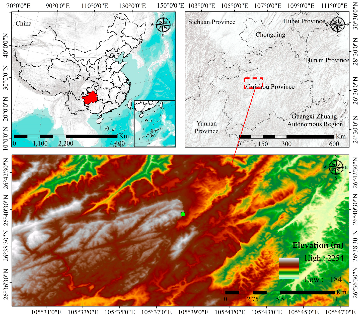
Figure 1. Location of rock slope.
Ijgi 14 00402 g001
Figure 2. Two typical rockslides in the study area: (a,b) represent the rockslides occurring on 28 August 2017 and 30 May 2024, respectively.
Ijgi 14 00402 g002
Figure 3. The deformation phenomena of the slope: (a) blocky structural configuration of the rock slope; (b) rock fragments resulting from the collapse at the base of the slope; (c) potential failure characteristics of rock slopes; (d) a close-up of a large tensile crack.
Ijgi 14 00402 g003
Figure 4. Computational principle of DEM.
Ijgi 14 00402 g004
Figure 5. Scheme of contact model: (a) contact model between individual elements; (b) schematic diagram of force calculation between individual elements.
Ijgi 14 00402 g005
Figure 6. Numerical model of the rock slope based on DEM: (a) remote sensing image of the slope (the data is from Google Earth); (b) three-dimensional numerical model.
Ijgi 14 00402 g006
Figure 7. The displacement contour map of potential rock failure.
Ijgi 14 00402 g007
Figure 8. The velocity contour map of potential rock failure.
Ijgi 14 00402 g008
Figure 9. Average movement velocity of the potential failure with time.
Ijgi 14 00402 g009
Figure 10. Average movement displacement of the potential failure with time.
Ijgi 14 00402 g010
Figure 11. Variation in kinetic energy of the sliding mass.
Ijgi 14 00402 g011
Figure 12. Variation in fracture energy of the sliding mass.
Ijgi 14 00402 g012
Figure 13. Variation in friction energy of the sliding mass.
Ijgi 14 00402 g013
Figure 14. Affected resident area of the potential rock failure.
Ijgi 14 00402 g014
Table 1. Parameters used in the numerical simulation.
Effective modulus (Pa)1 × 10⁸
Stiffness ratio2.5
Friction coefficient0.3
Normal bonding strength (Pa)3.6 × 10⁷
Tangential bonding strength (Pa)2.6 × 10⁷
Damping ratio0.5
Block size (m)0.5–9
Density (kg/m3)2750
Disclaimer/Publisher’s Note: The statements, opinions and data contained in all publications are solely those of the individual author(s) and contributor(s) and not of MDPI and/or the editor(s). MDPI and/or the editor(s) disclaim responsibility for any injury to people or property resulting from any ideas, methods, instructions or products referred to in the content.