Article

Exploration of Differences in Housing Price Determinants Based on Street View Imagery and the Geographical-XGBoost Model: Improving Quality of Life for Residents and Through-Travelers

1
International School of Engineering, Tianjin Chengjian University, Tianjin 300380, China
2
School of Architecture, Tianjin Chengjian University, Tianjin 300380, China
3
School of Architecture, Tianjin University, Tianjin 300072, China
*
Author to whom correspondence should be addressed.
ISPRS Int. J. Geo-Inf. 2025, 14(10), 391; https://doi.org/10.3390/ijgi14100391
Submission received: 16 August 2025 / Revised: 30 September 2025 / Accepted: 6 October 2025 / Published: 9 October 2025

Abstract

Street design quality and socio-economic factors jointly influence housing prices, but their intertwined effects and spatial variations remain under-quantified. Housing prices not only reflect residents’ neighborhood experiences but also stem from the spillover value of public streets perceived and used by different users. This study takes Tianjin as a case and views the street environment as an immediate experience proxy for through-travelers, combining street view images and crowdsourced perception data to extract both subjective and objective indicators of the street environment, and integrating neighborhood and location characteristics. We use Geographical-XGBoost to evaluate the relative contributions of multiple factors to housing prices and their spatial variations. The results show that incorporating both subjective and objective street information into the Hedonic Pricing Model (HPM) improves its explanatory power, while local modeling with G-XGBoost further reveals significant heterogeneity in the strength and direction of effects across different locations. The results indicate that incorporating both subjective and objective street information into the HPM enhances explanatory power, while local modeling with G-XGBoost reveals significant heterogeneity in the strength and direction of effects across different locations. Street greening, educational resources, and transportation accessibility are consistently associated with higher housing prices, but their strength varies by location. Core urban areas exhibit a “counterproductive effect” in terms of complexity and recognizability, while peripheral areas show a “barely acceptable effect,” which may increase cognitive load and uncertainty for through-travelers. In summary, street environments and socio-economic conditions jointly influence housing prices via a “corridor-side–community-side” dual-pathway: the former (enclosure, safety, recognizability) corresponds to immediate improvements for through-travelers, while the latter (education and public services) corresponds to long-term improvements for residents. Therefore, core urban areas should control design complexity and optimize human-scale safety cues, while peripheral areas should focus on enhancing public services and transportation, and meeting basic quality thresholds with green spaces and open areas. Urban renewal within a 15 min walking radius of residential areas is expected to collaboratively improve daily travel experiences and neighborhood quality for both residents and through-travelers, supporting differentiated housing policy development and enhancing overall quality of life.

1. Introduction

With the accelerating process of urbanization, over 55% of the global population now resides in urban areas, and this proportion is expected to increase to 68% by 2050 [1]. Future urban growth will primarily occur in developing countries, leading to an increased demand for housing [2]. Urban expansion not only intensifies the demand for housing but also raises the requirements for the quality of the living environment. As a core issue related to people’s livelihoods, housing in urban areas has long faced inequality due to factor agglomeration [3]. Housing prices are not only influenced by factors such as employment opportunities, accessibility to public facilities, and quality of life but also, to some extent, reflect these socio-economic disparities [4], which can be used to identify urban development patterns and support livability-oriented policies [5]. Although housing prices are not a direct measure of livability or environmental equity, their spatial distribution can indirectly reflect residents’ assessments of living environment quality. Existing studies struggle to explain how these disparities manifest in different regions and contexts, particularly in rapidly urbanizing cities in developing countries. Therefore, it is crucial to comprehensively assess how multi-level factors influence the distribution of urban housing prices.
The spatial imbalance of urban housing prices is particularly evident in the contrast between central and non-central districts [6,7]. Existing research typically characterizes these significant differences from three attributes: structure, neighborhood, and location [8,9]. At the structural level, features such as area, building age, floor, and apartment type influence prices. Simultaneously, location and accessibility-related factors (e.g., distance to the CBD, functional and economic activity clusters, and accessibility to public services such as education, healthcare, and leisure) have been repeatedly validated [10,11,12,13]. The supply of environmental and open spaces, as well as residents’ and through-travelers’ subjective impressions of the environment, have also been observed to be related to price differentiation [14,15]. Although these factors can explain the macro-level differences within the city, a significant “explanation gap” remains at the fine-grained level: on one hand, commonly used location and accessibility measures are often mid-to-macro indicators, which fail to capture the micro-environmental cues that residents and through-travelers encounter during their travel and stay [16,17]; on the other hand, the spatial scales of statistical units and perceived behaviors are inconsistent, often masking the heterogeneity at the parcel and interface levels at district or street scales, leading to a mismatch between “variables and behavioral pathways” [18]. While existing research can identify price differentiation, it struggles to answer which perceivable environmental features drive these differences, where they are most significant, and why they occur. Based on this, it is necessary to introduce environmental representations that are directly linked to actual experiences at the micro scale to enhance the explanatory power of fine-grained price differences.
How people perceive streets can influence their daily travel experiences and neighborhood evaluations, which in turn enter the housing price formation mechanism (i.e., “visual capital”) [19]. Street views not only reflect objective environmental quality but also influence spatial differences through the subjective perceptions of residents and through-travelers. For example, Ferreira et al. [20] demonstrate that at the street scale (e.g., street width and interface continuity), risk perceptions related to visibility and exposure vary with pedestrian and vehicular flow, leading to divergent experiential outcomes that affect the daily experiences of pedestrians, cyclists, bus passengers, and drivers [21]. Street view assessments typically combine both objective and subjective indicators: the objective side primarily measures greening, visibility, and other metrics [17,22,23,24], while the subjective side supplements with dimensions such as imaginability, complexity, human scale, and safety [15,25]. However, physical elements and perceptions are not always directly aligned, and solely relying on objective measurements cannot fully cover the complex mapping relationships [26,27,28]. The four dimensions of urban design—imaginability, complexity, human scale, and recognizability—reveal the differential experiences people have when recognizing, understanding, and using streets. Particularly in the context of pedestrian and cycling safety, perceptions of safety are closely related to path choices, willingness to stay, and neighborhood evaluations [15]. Since street views form a public visual interface along streets, in addition to residents, through-travelers are also key audiences. Therefore, enclosure, safety, and recognizability can be understood as “corridor-side” exposure cues, complementing the neighborhood factors’ perspective. Research on human perception in housing prices has traditionally focused on homebuyers’ assessments of the surrounding environment. Existing studies often use crowdsourced data like Place Pulse to capture emotional dimensions [29,30], but such datasets are insufficient for covering cities in mainland China and have significant contextual differences [31]. Recent studies have begun to construct resident perception data based on local SVI and incorporate city design-oriented dimensions (imaginability, complexity, human scale, and recognizability) [15,25], to more closely reveal the mechanisms by which street perception differences affect housing value in a local context, while considering both residents’ and road users’ perceptions, thus providing new empirical support for urban design and housing policy.
The Hedonic Pricing Model (HPM) is widely used to quantitatively identify the value contribution of housing attributes by decomposing prices into quantifiable factors such as structure, neighborhood, and location. Empirical evidence on street-level information has been preliminarily accumulated through this approach [32,33,34,35]. Objective environmental elements (e.g., greening, landscape openness) have been empirically shown to have premium associations in various locations. For instance, Michael [36] found that blue-green spaces have a premium effect on housing prices by evaluating urban facilities. Ye [37] found a significant positive correlation between street greening, street accessibility, and housing prices, with street greening achieving the second-highest coefficient in the HPM model. Chen [38] found a nonlinear relationship between housing prices and GVI in Shanghai. Subjective dimensions related to actual experiences (such as safety) also show stable positive relationships [39]. Further comparative studies indicate that subjective and objective representations are not simple substitutes in explaining price differences; they may complement each other or present inconsistent directions for individual factors. Xu [15] measured six perceptions (greenness, safety, walkability, imaginability, enclosure, and complexity) both subjectively and objectively, and found that the collective strength of subjective scores and their objective counterparts was almost equal. Both subjective and objective indicators showed opposite individual tendencies in explaining price differences, and perceptions cannot be fully represented by objective indicators. Building on this, there is still room for further investigation into how to assess their incremental explanatory power and relative effects within the same quantitative framework, and how these factors manifest differently within the city.
To fairly compare the incremental explanatory power and relative effects of subjective and objective street elements within the same quantitative framework, and to identify their differentiated manifestations within the city, the key lies in the choice of econometric implementation. In pursuit of this goal, existing empirical research typically uses the Hedonic Pricing Model (HPM) as the basis, with differences primarily in the implementation of parameter estimation and spatial treatment. In HPM empirical modeling, Ordinary Least Squares (OLS), due to its simplicity and interpretability, is widely applied in housing price regression analysis. However, the uniform coefficient assumption can obscure relationship differences across locations and introduce the risk of reversal due to aggregation in the handling of geographical data (the “Simpson’s Paradox”) [40]. To address this issue, Geographically Weighted Regression (GWR), as a local modeling method, has been widely used to reveal variations in variable relationships under spatial heterogeneity [41]. Unlike the global OLS model, GWR allows model parameters to vary with geographical location and estimates a set of local regression coefficients for each observation point, thus better capturing spatial non-stationarity [42]. However, its linear nature still makes it difficult to capture nonlinear structures and higher-order interactions between variables, and it is sensitive to settings like bandwidth. In recent years, researchers have begun integrating machine learning with spatial modeling, developing methods such as Geographical Perception Random Forest (Geo-RF) and Geographically Weighted Gradient Boosting Trees (Geo-XGBoost), which retain the local modeling concept while introducing non-parametric learning capabilities to effectively capture nonlinear features, variable interactions, and heterogeneous distributions in spatial processes [43,44]. Therefore, the application of nonlinear geographical algorithms in housing price research can reduce Simpson’s Paradox and address spatial heterogeneity, thereby providing a more accurate understanding of the economic benefits of environmental policies and their spatial distribution characteristics. Based on this, this study adopts Geographical-XGBoost to compare the relative effects of subjective and objective street elements within the same framework and to characterize their heterogeneity within the city.
This study aims to provide a comprehensive assessment of the factors influencing housing prices by integrating multi-source data and machine learning algorithms. Using local Street View Imagery (SVI) as a basis, the study compares the complementary roles and relative importance of objective views and subjective visual perceptions. In this study, we take Tianjin, China, as a case study and use locally collected SVI to train a perception scoring model that predicts human perceptions of the street environment. A deep learning model is employed to segment the SVI and extract objective view indices. Additionally, a geographically weighted nonlinear method is introduced to relax traditional linear assumptions, enabling a better explanation of the spatial heterogeneity and impact differences of housing price determinants. The study quantifies and reveals the incremental explanatory power of both subjective and objective street view variables on housing prices and their spatial differences, further demonstrating the interplay and heterogeneity of influencing factors across different regions.
This study makes three main contributions. First, it integrates local SVI subjective and objective information with a geographically weighted nonlinear approach to quantify the perceptible link between street view elements and housing price signals across different locations, revealing their spatial heterogeneity and relative effects. This provides empirical evidence for understanding the interplay and differences in housing price determinants within the city. Second, without being confined to a single linear assumption, this study offers a replicable assessment framework to identify spatial heterogeneity and enhance explanatory power, providing references and priority judgments for evidence-based, zoned housing and street renewal. This study transforms the concept of a “good street” from an abstract judgment into quantifiable design clues, and, through housing prices as a market signal, tightly links changes in street view features with improvements in the quality of life for residents and through-travelers. Third, by incorporating the differences in human perceptions of the street environment into the analysis, it highlights the planning implications of equity and experience, enriching traditional urban design and policy evaluation. It should be noted that this study does not claim causal conclusions; our goal is to assess the incremental explanatory value of micro-level street view information in existing housing price models, aiming to provide interpretable evidence to support the improvement of livability and service accessibility, enhance the walking experience for residents and through-travelers (e.g., bus passengers, cyclists, and electric two-wheeler riders), and promote more equitable spatial resource allocation.

2. Study Area and Data

2.1. Study Area

There are significant differences in street configurations and interface morphology between the core and suburban areas of Tianjin, primarily reflected in the variations in vehicular, pedestrian, and cycling spaces, as well as commercial interfaces. The core area (Heping, Hexi, Nankai, Hedong, Hebei, Hongqiao) features a framework of multi-lane main roads and narrower secondary roads (main roads typically have 6–8 lanes, with sidewalks 3–5 m wide). Street trees and protected cycling facilities are commonly found, and commercial corridors are lively. Parallel parking is mainly seen on secondary roads. Suburban areas (Dongli, Xiqing, Jinnan, Beichen), as the primary zones for urban expansion, have more diverse street forms with larger setbacks (the distance from the building to the sidewalk is about 5–10 m). There is a higher proportion of newly planted street trees, and sidewalks are wider, but the continuity of protected cycling lanes is relatively weaker. Buildings are primarily high-rise residential complexes, with discontinuous street walls and more open space, creating a clear distinction from the core area.
This study focuses on the central urban districts (the six districts within the city) and suburban areas (the four districts surrounding the city) of Tianjin, a municipality directly under the central government of China, as the empirical study area Figure 1. Tianjin is located in the northern part of the North China Plain, between 116°43′ to 118°04′ East longitude and 38°34′to 40°15′ North latitude, making it an important economic and port city in northern China. In 2020, the total area of Tianjin was approximately 11,966 square kilometers, with a permanent population of about 13.82 million and an urbanization rate of 82.57%. In the rapid process of urbanization, Tianjin has formed a distinct “core–periphery” spatial structure, which is particularly evident in the differentiation between central and non-central urban areas. This study focuses on these ten districts, using street view images (SVI) and housing price data collected on-site, to reveal the differentiated patterns of housing price determinants in both regions. This serves as a typical case to support the analysis of how urban visual environments affect the spatial distribution of housing prices.

2.2. Research Framework

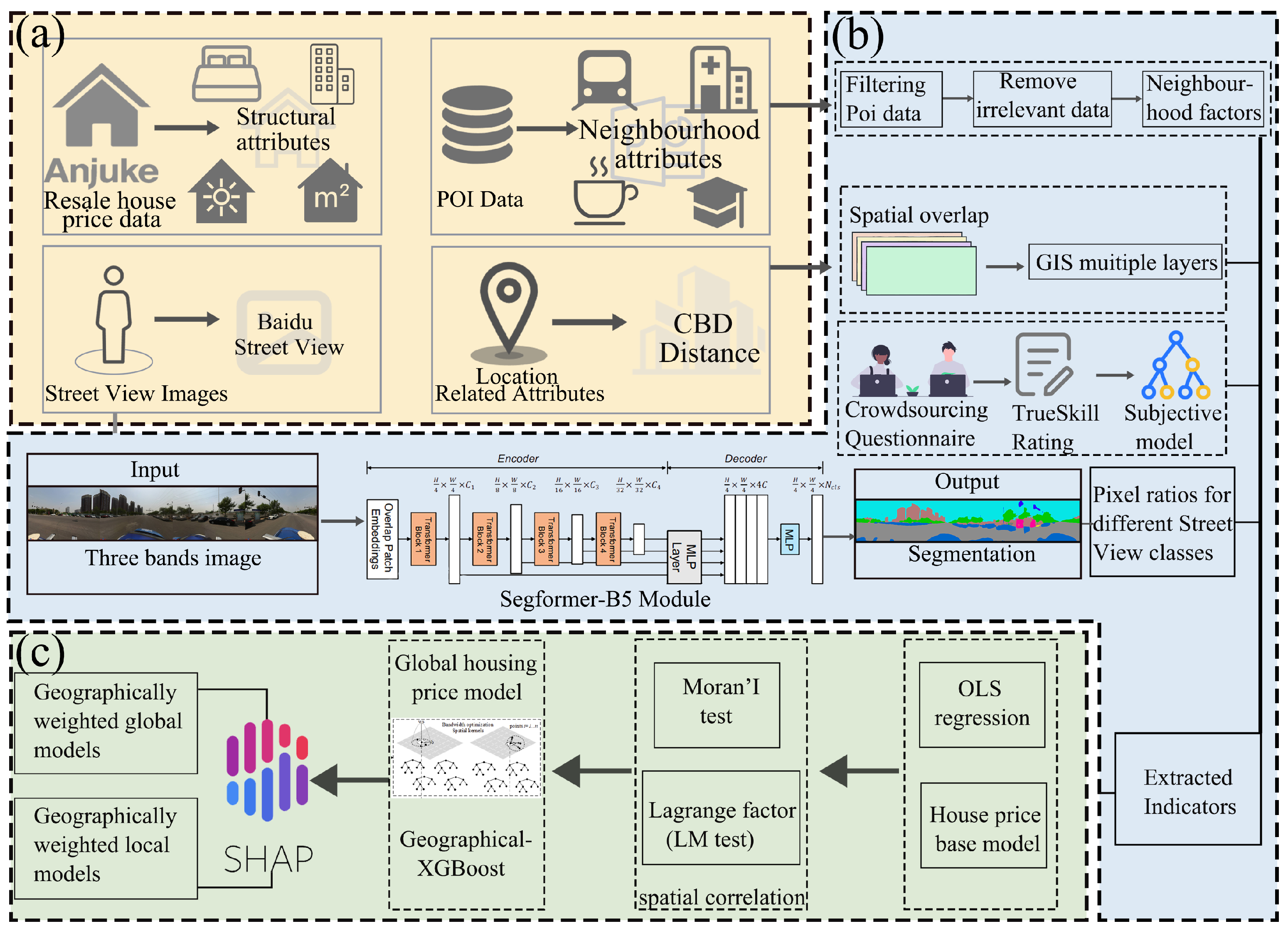
The main steps of the research framework are outlined below, as shown in Figure 2, summarizing the workflow of this study, which includes data collection, feature extraction, property price modeling, and analysis. First, we collected a multi-source dataset consisting of street view images, Points of Interest (POI), neighborhood information, and basic property attributes. Second, we extracted multiple features from these datasets and collected subjective perception scoring data from 45 participants in Tianjin through a crowdsourced visual survey. Third, we established a basic property price model using Ordinary Least Squares (OLS) and tested spatial autocorrelation, dependency, and potential spatial heterogeneity using Moran’s I test and the Lagrange multiplier test on its residuals. We then explored the spatial relationships between property prices and related factors using Geographical-XGBoost (version 1.0.9). Finally, we compared the impact of property price determinants on property prices, considering geographical location, using the global model. We also analyzed the strength of these determinants through SHAP interpretability analysis, and visualized the spatial heterogeneity of the study area using SHAP values from the local model.

2.3. Data

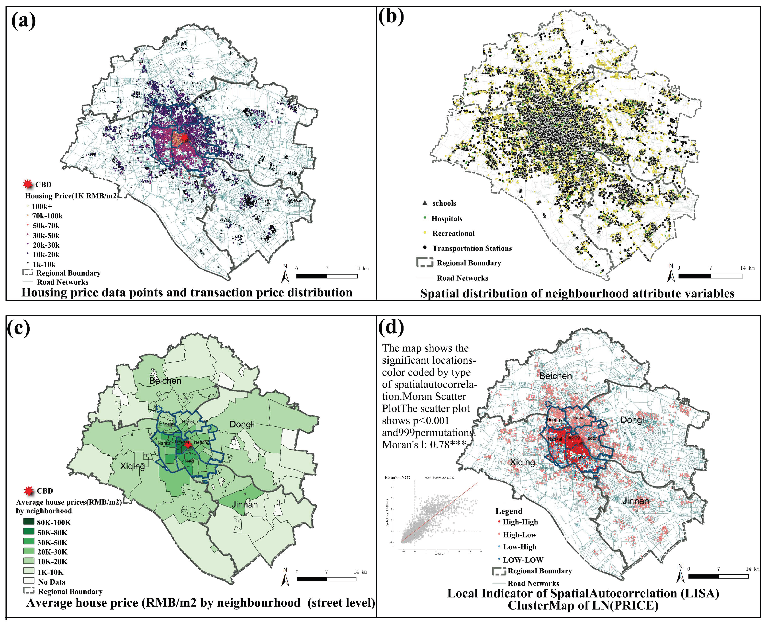
Table 1 provides the descriptive statistics for all the variables used in this study. As of December 2024, the data for this study was collected through web scraping techniques from “Anjuke,” a leading real estate platform in China (https://tianjin.anjuke.com/, accessed on 3 May 2025), covering average listing prices of second-hand homes from 5100 communities in Tianjin (Figure 3a). Anjuke is a real estate information service platform covering 300 major cities across China and is one of the most popular real estate service providers in the country. Taking into account data availability and relevant literature [45,46], variables were selected and defined based on practical demand using automated web scraping.The structural attribute variables include property type (Property_T), building age (House_Age), year of construction (Year_Built), floor area ratio (Floor_Area), greening rate (Greening_R), building type (Building_T), and property fees (Property_F). Property type (e.g., regular residential, apartment) and building type (e.g., low-rise, mid-rise, high-rise) are categorical variables, which were converted into dummy variables using one-hot encoding to prevent information loss or bias in the model due to categorical variables. To ensure the consistency and representativeness of the sample, duplex apartments and villas were excluded from the study to avoid potential biases, thus enhancing the reliability of the results. Price refers to the average listing price of homes currently for sale in each community. Geographic coordinates of the residential communities were collected using the Baidu Map geocoding service, and the structural attributes were integrated with the property price data.
Furthermore, neighborhood attribute data primarily came from the Points of Interest (POI) data provided by Baidu Map (version 3.0), obtained through web scraping. According to the requirements of HPM modeling for neighborhood environments, this study extracted the following indicators from the POI data: the distance to the nearest subway and bus stations (HubDist), the number of schools (school_n), medical facilities (hospital_n), and recreational services (recreation_n) within a 1000 m radius around the residential points, using QGIS spatial analysis tools for calculation (Figure 3b); see Table 1. These indicators were used as core metrics to measure neighborhood accessibility and public service levels. Regarding location attributes, the shortest network distance from the residential area to the Central Business District (CBD) was introduced as a spatial centrality indicator. The CBD of Tianjin was defined as the Xiaobailou Commercial District in Heping District, which houses financial, commercial, and high-end office resources, representing the city’s main functional core. The distance from each community to the CBD was obtained using the road network from OpenStreetMap (OSM, https://www.openstreetmap.org/).

2.4. Street View Feature Extraction

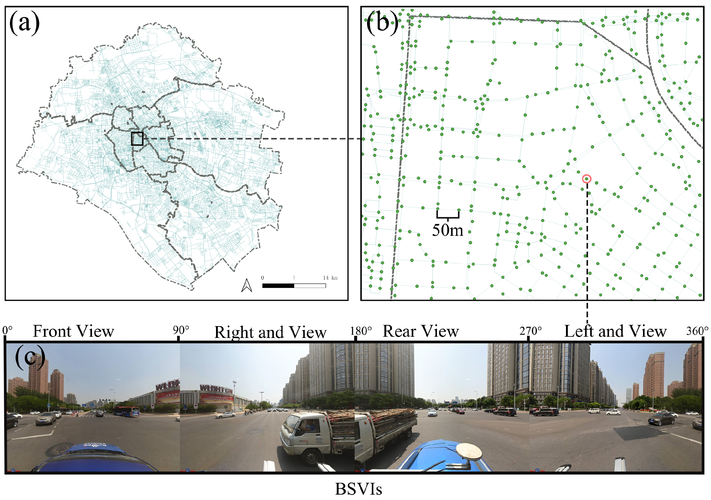
To capture both the subjective human perceptions and objective view indices of the street environment, this study employs the Street View Imagery (SVI) method for information extraction. The street view images are sourced from Baidu Maps, which, as one of China’s leading map service providers, offers an Application Programming Interface (API) that allows users to programmatically retrieve street view images in bulk, as shown in Figure 4. In this study, we first used Python’s OSMnx library (version 2.0.6) to obtain the UTM coordinate system road network data for the study area. Points were sampled at 50 m intervals, and the KDTree algorithm was employed to select street view points with a proximity of less than 50 m, resulting in a total of 143,956 candidate sampling points. Using Baidu’s geocoding API, the WGS84 coordinates were converted to BD-09 (Baidu’s coordinate system), with four collection directions (0/90/180/270°) for each sampling point. Images were stitched together, with each image having a resolution of 1024 × 768 pixels. We retained only the images captured from June to August 2023 and filtered them based on quality control standards such as location consistency and image clarity. Due to factors such as third-party street view supply and on-site conditions (e.g., areas without coverage, road closures/construction zones, temporary obstructions, or images outside the specified time window), the final dataset contained 74,324 valid panoramic images. These images adequately cover the main streets, various functional zones, and diverse street design characteristics of Tianjin’s central urban and suburban areas, ensuring spatial representativeness of the study area and comprehensiveness of the data.
This study employs the SegFormer-B5 model, based on the Transformer architecture, to extract semantic features from the Street View Imagery (SVI) [47]. SegFormer-B5 is part of the SegFormer series, specifically designed for efficient semantic segmentation tasks. By predicting the category label for each pixel in the input image and incorporating a pyramid pooling module to provide additional contextual information, SegFormer-B5 effectively avoids segmentation errors. This model has been widely adopted in various urban studies [48,49]. The ADE20K dataset, which includes street view data from 50 cities and annotations for 150 urban landscape object categories, was used as the training data for semantic segmentation of street view images [50].
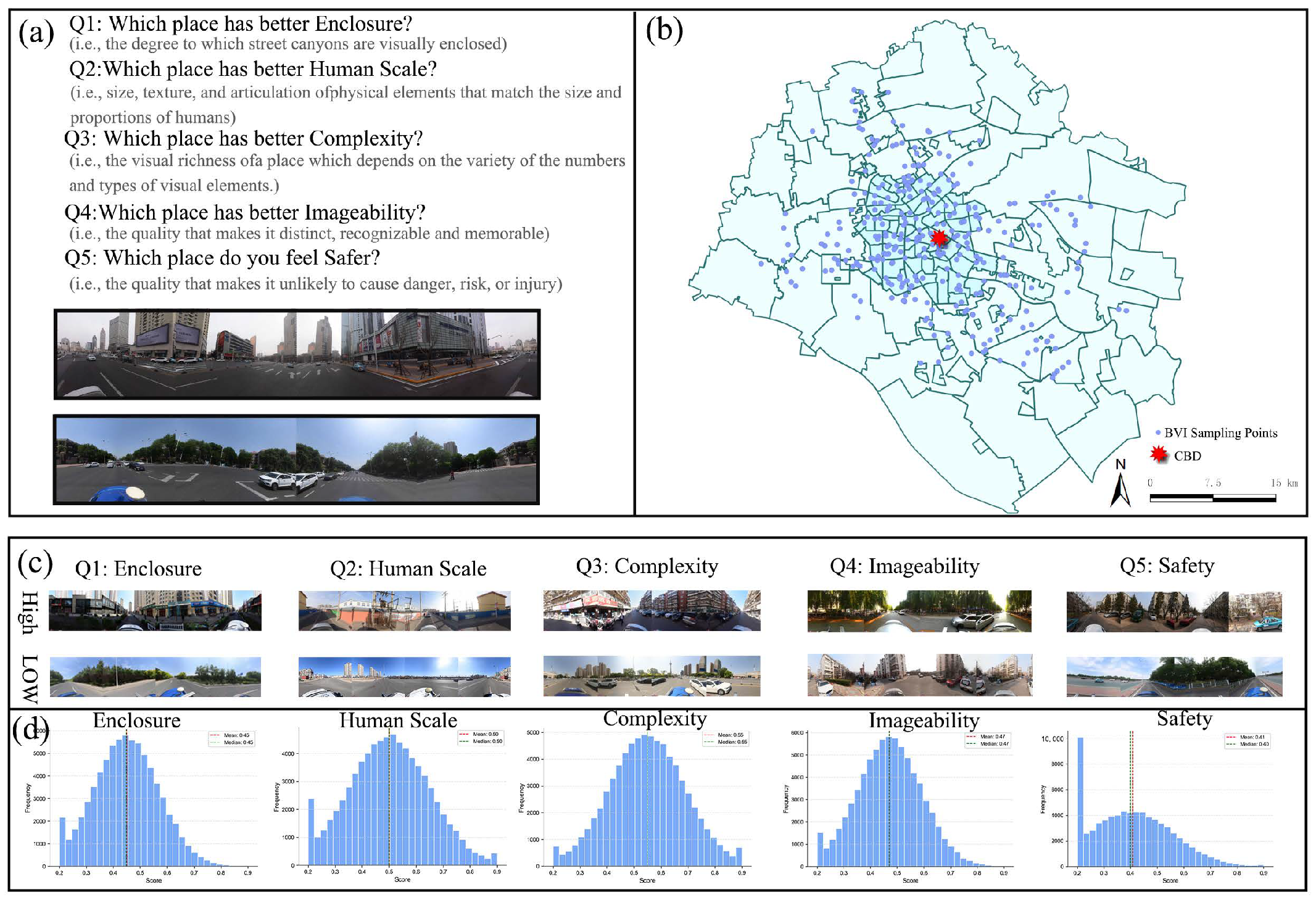
For the selection of subjective perceptions, this study draws on urban design theory [51] and selects four design qualities: “1. enclosure,” “2. human scale,” “3. complexity,” and “4. imageability.” In addition, we refer to the urban scene understanding from the Place Pulse project [52] and add “5. safety” as a perceptual dimension, as it has been shown to significantly influence residents’ behavior [16,53]. In total, five design qualities were chosen to measure subjective perceptions of street scenes. Inspired by Place Pulse 1.0 [54], we randomly sampled 300 SVIs to ensure coverage of both the six central urban districts and the four suburban districts in Tianjin, as seen in Figure 4b, and established a crowdsourced visual survey platform. Participants could choose a preferred photo from two randomly selected SVIs and answer questions such as “Which place has a better enclosure?” Each question provided a clear qualitative definition; the evaluation process was double-blind, with the geographic location of the images not revealed (Figure 5a). Since non-expert pedestrians may have a vague conceptual understanding of the five design qualities, this study involved participants with relevant training backgrounds to conduct pairwise comparison assessments, in order to reduce measurement noise and ensure construct validity. A total of 45 master’s-level urban design researchers participated (26 males, 19 females; average age = 24). Participation was voluntary and anonymous, with informed consent obtained prior to participation. No personally identifiable information was collected. The TrueSkill Bayesian scoring system was used to convert pairwise votes into ranking scores. This system generates scores for winners and losers after each comparison, and standardizes the scores to a 0–1 range. The results from the 300 SVIs were used to construct and evaluate the perceptual prediction model [55,56]. Furthermore, the dataset achieved a passing rate of over 75%, indicating good internal consistency of the manual ranking process. Each SVI was compared between 20 and 36 times on average (Figure 5c), and a total of 4321 pairwise ratings were collected (Figure 5d). Compared to similar studies, the results are reliable [55,56].

3. Methodology

3.1. Housing Price Models

The Hedonic Pricing Model (HPM) conceptualizes housing as a heterogeneous good, with its price determined by three main attributes: structure, location, and neighborhood attributes. Structural attributes describe the physical characteristics of the property itself (e.g., building area, age, building type). In empirical analysis, it is necessary to include structural attributes as control variables in the model to ensure that the effects of the street environment are more reliably identified. Location attributes refer to the geographical position of the property within the city, reflecting accessibility and spatial advantages. Neighborhood attributes reflect the accessibility of essential facilities and services around the property. In this study, recognizing the growing importance of street environment quality and perceptual experiences in urban research, we extend the HPM framework. Although subjective perception scores and objective view indices are considered part of the neighborhood attributes, in order to more systematically assess the impact of street environment quality on housing prices, we classify them into a new attribute group, referred to as STRE. The STRE group captures the public interface along streets through SVI, with its exposed subjects not only including residents but also through-travelers (e.g., bus passengers, cyclists, and commuter drivers). This group reflects both residential experiences and the influence of high-frequency exposure on price formation. The HPM is extended as shown in Equation (1).
PRICE = α + β 1 STRU + β 2 LOCA + β 3 NEIG + β 4 STRE + ε
where α represents the constant term; β 1 to β 4 represent the attributes of structural (STRU), location (LOCA), neighborhood (NEIG), and street environment perception (STRE); and ε represents the error term.
To assess the independent explanatory power of each type of variable on housing prices, we first include the five groups of variables separately in individual OLS models for preliminary testing. It should be noted that OLS theoretically assumes the error term is independently and identically distributed, with no spatial correlation. However, in urban spatial data, this assumption is often violated due to spatial dependence and spatial heterogeneity, which may lead to biased coefficients and distorted significance tests [57]. Nevertheless, OLS is still widely used as the starting model, serving three main purposes: (1) OLS provides a benchmark framework for comparing subsequent spatial regression models; (2) Moran’s I and Lagrange multiplier tests, calculated from the OLS residuals, provide theoretical justification for introducing spatial interaction terms; and (3) OLS is simple and efficient, allowing for the preliminary identification of key factors, guiding variable selection, and offering early predictions of potential multicollinearity or specification issues in spatial regressions. To avoid multicollinearity interfering with regression results, we conducted a Variance Inflation Factor (VIF) test and excluded variables with a VIF value exceeding 10 and weak explanatory power [58]. Next, a baseline model was constructed using structural, location, and neighborhood attributes, with insignificant variables ( p > 0.05 ) removed, in order to measure the explanatory power of the traditional HPM framework on housing prices. For instance, the “distance to subway and bus stations” was removed due to its weak explanatory power and high correlation with neighborhood attributes. Based on the baseline model, the five types of subjective perception scores and the seven objective view index indicators, classified according to urban morphology, were added to systematically compare the explanatory power differences of street environment quality in housing price modeling. To detect spatial effects, Moran’s I and Lagrange multiplier tests were performed on the OLS residuals to verify the spatial autocorrelation and spatial dependence of the residuals.

3.2. Geographical-XGBoost

Geographically Weighted XGBoost (G-XGBoost), as proposed by Grekousis Grekousis [59], is used in this study to address the limitations of Geographically Weighted Regression (GWR) and its semi-parametric extension (SGWR). Although GWR and SGWR have significant advantages in revealing spatial non-stationarity of variables, they rely on linear assumptions and struggle to capture nonlinear relationships and higher-order interactions, which limits their ability to handle complex spatial relationships [59]. To overcome these limitations and capture both the overall trend of housing price determinants and local spatial heterogeneity, this study adopts the G-XGBoost model, which combines the nonlinear modeling capabilities of XGBoost with the local regression mechanism of geographically weighted modeling. By introducing spatial weights, constructing local sub-models, and integrating global and local prediction frameworks, G-XGBoost effectively models the spatial heterogeneity of feature–response relationships. In G-XGBoost, the traditional XGBoost model is used as the global model to capture the overall nonlinear trend of housing prices. The model improves predictions by adding trees iteratively in a “tree-by-tree” manner: in each round, a new regression tree f t is learned to minimize the error of the current prediction. The training objective is given by Equation (2):
L ( t ) j = 1 N g j f t ( x j ) + 1 2 h j f t ( x j ) 2 + Ω ( f t )
where g j represents the direction and magnitude of error change when adjusting the prediction for sample j (first-order information), h j reflects the curvature of the error surface (second-order information), f t is the output increment of the new regression tree in the current round, and Ω ( f t ) is the regularization term (to prevent overfitting by limiting the number of leaves T and the leaf values). After multiple iterations, the global model’s prediction is represented as the sum of several trees, as shown in Equation (3):
y ^ i gl = k = 1 K f k ( x i ) , f k F
where y ^ i gl is the global prediction for sample i, f k is the k-th CART regression tree, K is the total number of trees, and F is the set of all possible regression trees. The global model is estimated without spatial weights to capture the overall nonlinear relationship at the city scale and serves as the benchmark for subsequent local (geographically weighted) modeling to capture spatial heterogeneity. In this unified optimization framework, spatial kernel weights ( w i j 0 ) are used to adjust sample contributions to reveal spatial heterogeneity. G-XGBoost builds local models within the neighborhood of each spatial unit i, and the optimal bandwidth b is selected via cross-validation (CV). Using w i j as instance weights, the first- and second-order terms of the standard XGBoost objective Equation (2) are introduced to derive the local objective function, as seen in Equation (4):
L i loc = j = 1 n i g j · w i j · f t ( x j ) + 1 2 h j · w i j · f t 2 ( x j ) + Ω ( f t )
where g j and h j are the first- and second-order gradients, and f t ( x j ) is the prediction of the t-th regression tree for sample j. The regularization term Ω ( f t ) is included to prevent overfitting. This weighted second-order objective function is isomorphic to the standard XGBoost model: the solution method remains unchanged, except that the summation over samples is replaced by a spatially weighted summation (which degrades to global XGBoost when w i j 1 ). The optimal leaf values and split gains for the local tree are then given by Equation (5):
w u * = j I w i j g j λ + j I w i j h j , Gain = 1 2 G L 2 λ + H L + G R 2 λ + H R G T 2 λ + H T
where G ( · ) = j ( · ) w i j g j , H ( · ) = j ( · ) w i j h j . Optionally, to enhance comparability between different neighborhood scales, j N ( i ) w i j = 1 (row normalization) can be applied. When w i j 1 (or the neighborhood covers all samples), Equation (4) degrades to the global XGBoost objective and solution process. Unlike the original XGBoost, G-XGBoost embeds spatial weights directly into the gradient calculations, making the model focus more on nearby samples that contribute more to prediction errors during training. Finally, G-XGBoost dynamically integrates global and local predictions using a weighted coefficient α i [ 0 , 1 ] , as seen in Equation (6):
y ^ i ens = α i y ^ i loc + ( 1 α i ) y ^ i gl , α i [ 0 , 1 ]
where α i can be a constant or adaptively adjusted based on local and global residuals: when the local model error is large, α i is reduced to emphasize global information; conversely, α i is increased to better capture fine-grained spatial heterogeneity.
To transparently identify the “Street View–Housing Price” mechanism within a nonlinear learning framework, this study combines the global G-XGBoost (Equations (2) and (3)) and local G-XGBoost (Equation (4)) with the SHAP (SHapley Additive exPlanations) interpretability framework. This approach analyzes the contribution and impact of various features on the model’s predictions, thereby enhancing the model’s interpretability and comprehensibility. SHAP improves the transparency of “black-box” models by calculating the marginal contribution of each feature to the model’s output, offering insights into feature importance from both global and local perspectives. Each feature is treated as a “contributor” to the prediction, with its value reflecting the positive or negative influence of that feature on the prediction for a specific instance, providing an intuitive and quantifiable explanation mechanism [60]. Following the method proposed by Li [60]. For data processing, we split the dataset into 70% training and 30% testing sets to ensure model robustness and generalization ability. During the training phase, we used nested cross-validation combined with grid search to select key hyperparameters for the global G-XGBoost model, thereby reducing overfitting and improving generalization performance. Subsequently, adaptive kernels were used to systematically search for the optimal bandwidth within a given range and fix it at the best value. Finally, we trained the local models using spatial weights and a weighting strategy with variable strength coefficients.
The local G-XGBoost model introduces spatial weights when calculating feature importance, which results in a weighted correction of XGBoost’s “gain” metric, yielding spatially weighted feature importance. This allows us to quantify the contribution differences of each feature across different locations. Unlike the traditional parametric linear framework of Geographically Weighted Regression (GWR), the local model of G-XGBoost is a non-parametric tree ensemble: for each spatial location, a set of local tree structures is fitted under a given bandwidth and weight. The prediction function consists of a piecewise nonlinear combination of multiple trees. Therefore, this framework does not generate linear coefficients and cannot directly produce a “coefficient map” like GWR. To bridge this interpretative gap, we adopt SHAP as a unified interpretability layer: it precisely quantifies the positive or negative marginal contribution of each feature to the prediction at the single-sample level, and spatial visualizations are generated based on these contributions. The Shapley value for local G-XGBoost at each sample’s geographic location i is calculated as Equation (7), and its spatial visualization results replace the regression coefficient map of the traditional GWR model. Compared to traditional feature importance metrics, SHAP has the advantages of consistency and additivity. It not only reflects the relative importance of features in the overall model but also reveals the local effect differences of these features across different geographic locations.
f s loc ( x i ) = ϕ 0 , s + j = 1 p ϕ i j ( loc , s ) , ϕ 0 , s = k N ( s ) w s k f s loc ( x k ) k N ( s ) w s k
In the local model at location s, the prediction for sample i is the sum of the “local weighted baseline” ϕ 0 , s and the local SHAP contributions of each feature, where ϕ 0 , s is the weighted average of the local predictions f s loc ( x k ) using neighborhood weights w s k . To further reveal spatial heterogeneity and nonlinear contributions within the city, we calculate the Shapley values at the sample level { ϕ i j } on the global G-XGBoost model (Equations (2) and (3)) and perform comparisons at the regional level: we calculate the regional importance for the six central urban districts and the four suburban districts, as shown in Equation (8):
Imp j , r = 1 N r i r ϕ i j ( gl )
Equation (8) defines the “regional importance” metric: for region (or sub-sample) r, we take the absolute value of the global SHAP values ϕ i j ( gl ) of feature j for all samples i in region r and average them to obtain the average marginal impact of that feature on the prediction within the region. This quantifies the relative strength and ranking of the dominant factors in different regions, thus identifying inter-regional differences in the “Street View–Housing Price” mechanism. Further, to identify nonlinear marginal effects and their potential thresholds, we visualize and test the dependency relationship between ( x i j , ϕ i j ) across the entire region, thereby characterizing the nonlinear response of feature value changes on prediction contributions.

3.3. Subjective Perception Modeling

The training data for the perception model comprise 300 SVIs obtained from an online visual survey, with five ranked perception scores serving as labels and view indices extracted from street view images as explanatory variables. The dataset was split into training and test sets using an 80/20 split [61]. Among tree-based models, this study adopts the Random Forest (RF) algorithm, as previous research has demonstrated its high predictive accuracy and robustness in urban scene perception modeling [62]. For example, Yao et al. [63] successfully employed an RF model to fit and predict expert-assessed perception scores, achieving favorable results. Following this approach, the present study trains a separate RF model for each subjective perception category. Model performance is evaluated using the coefficient of determination ( R 2 ), mean absolute error (MAE), and root mean square error (RMSE). Following the framework proposed by [64], an MAE within 10% of the range of the training data is considered indicative of good predictive ability Equation (9), whereas an error exceeding 25% suggests that the model or data may require re-evaluation (Equation (10)). The best-performing model is then used to predict subjective perception scores for the remaining 74,324 unrated SVIs and to calculate the average perceived score for all SVIs within a 1 km radius (equivalent to a 15 min walking distance) of each residential location.
MAE 0.1 × trainingsetrange , AND , MAE + 3 × std . dev . 0.2 × trainingsetrange
MAE > 0.15 × trainingsetrange , OR , MAE + 3 × std . dev . > 0.25 × trainingsetrange
To assess the relative importance of different street scene features in prediction, we employed the Gini Importance (GI) index to quantify each feature’s contribution within the Random Forest model, computed using the Scikit-learn library. Based on the objective view indices from the perception model training results and the GI values of subjective perceptions, the top 20 feature categories were aggregated into seven urban morphological indicators, which were subsequently used as explanatory variables. The proportion for a single category was calculated as follows in Equation (11):
V o b j = i = 1 m A r e a o b j i i = 1 m A r e a t o t a l i × 100
where A r e a o b j i denotes the number of pixels corresponding to a specific object (e.g., buildings, sky, or trees) in the i-th street view image, obtained via a deep learning-based semantic segmentation algorithm; A r e a t o t a l i represents the total number of pixels in the entire image; and m is the total number of SVIs.
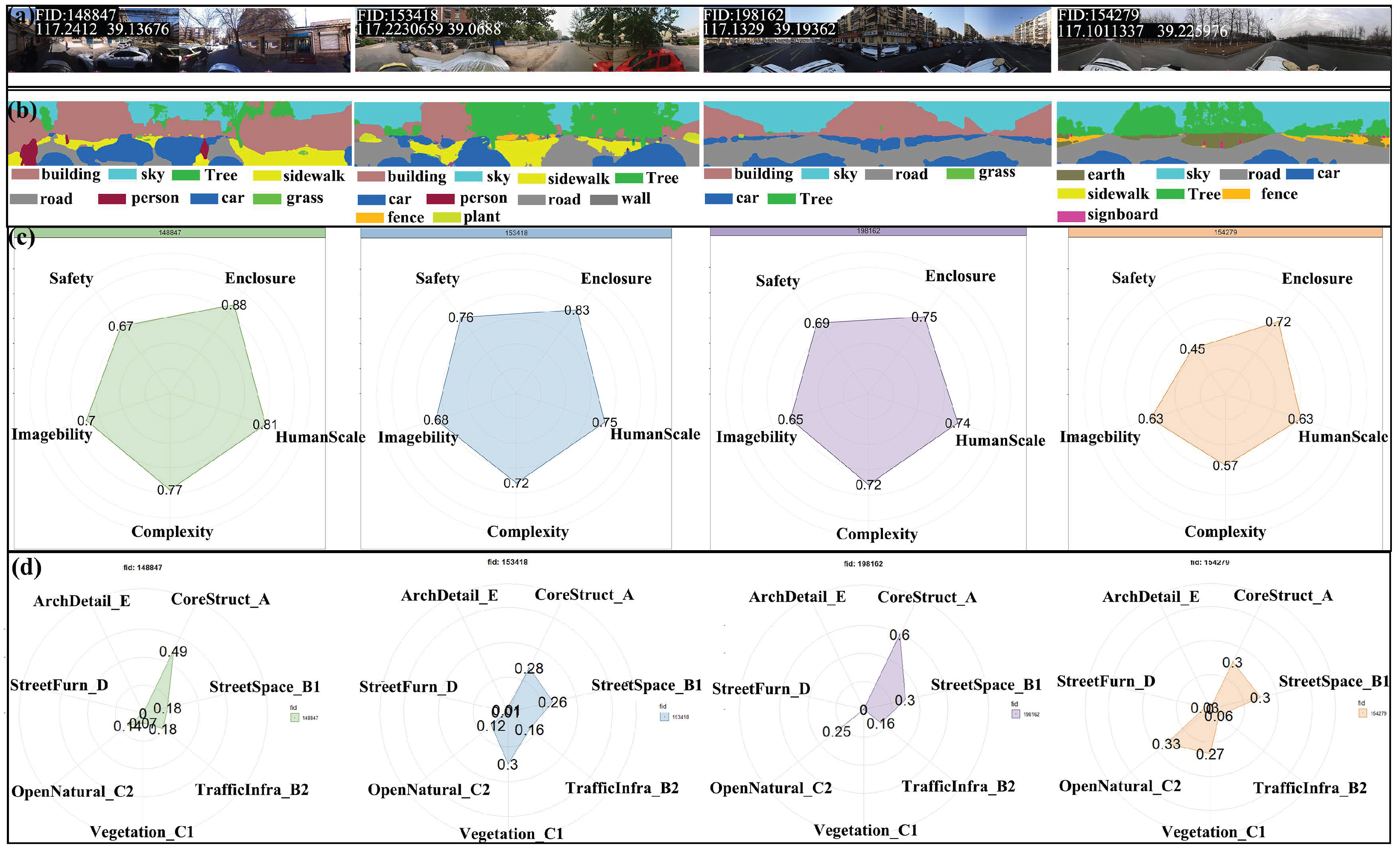
Given that subjective perceptions may exhibit strong intercorrelations—for instance, Zhang et al. [65] found that "repression–safety" and "beauty–wealth" perceptions are highly correlated—we calculated the Pearson correlation coefficients between the five subjective perception scores and the seven morphological indicators to identify and mitigate multicollinearity. In selecting explanatory variables for the HPM model, variables with strong correlations and high variance inflation factors (VIF) were excluded to avoid multicollinearity in the regression analysis. Finally, to validate the reliability of the results, we randomly selected four SVIs and manually inspected their original images, segmentation outputs, and corresponding score distributions [66,67].

4. Results

4.1. Modeling and Spatial Analysis of Street Perceptions

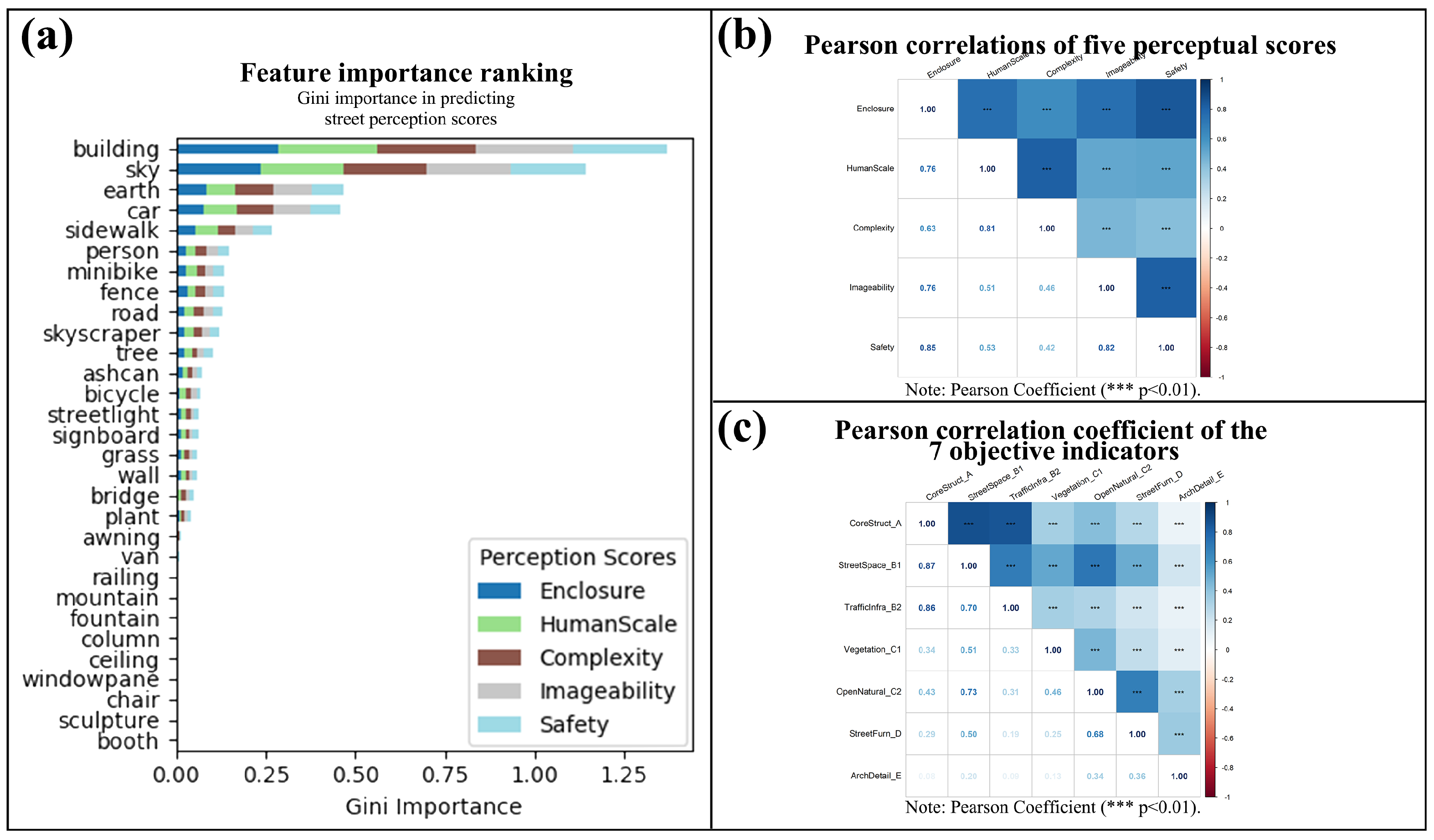
Table 2 shows the Gini Importance of 30 objective view indices for five perceptions in training the perception prediction model. Combining the outputs of the perception model with urban morphological theory [68], it is evident that not all visual elements have a significant impact on perception scores. Therefore, based on theGini Importance ranking (Figure 6a), we selected the top twenty most explanatory visual elements and classified them into seven street view spatial groups: Core Building (CoreStruct_A), Street Space (StreetSpace_B1), Traffic Flow (TrafficInfra_B2), Vegetation (Vegetation_C1), Open Nature (OpenNatural_C2), Street Furniture (StreetFurn_D), and Architectural Details (ArchDetail_E). These indices were then incorporated into the HPM model, along with subjective perception scores, to compare their explanatory power on housing prices. In the usage context, StreetSpace_B1, TrafficInfra_B2, CoreStruct_A, and ArchDetail_E primarily serve as “corridor-side” exposure elements, while Vegetation_C1, OpenNatural_C2, and StreetFurn_D carry signals related to neighborhood livability and travel comfort. Together, they provide explanatory value for the experiences of both residents and through-travelers.
Figure 7 presents the validation results on randomly selected SVI samples. Different SVIs exhibit distinct perception scores and view indices, confirming the accuracy of various visual elements in street scene perception. The first and third images show high “enclosure” scores when CoreStruct_A scores are high, while the second and fourth images display significant “safety” differences, more clearly influenced by the combined effect of “Open Nature” (OpenNatural_C2) and “Traffic Flow” (TrafficInfra_B2). The last three images perform similarly in human scale and imaginability dimensions, or are related to the “Street Space” (StreetSpace_B1) structure. Analyzing all four images, the average scores and variance increase with higher “enclosure” and “safety” scores, as shown in Figure 7c,d. The results indicate that well-defined perception dimensions, particularly “enclosure” and “safety,” show higher distinguishability and lower prediction error in our model. This may reflect stronger preferences in the visual assessments of residents and street users. Corridor-side elements (such as clearer sightlines and more stable enclosure) provide more discernible safety and predictability cues for through-travelers, thereby influencing their experience and evaluation across street segments.
The specifications of the perceptual prediction model and the prediction performance for each perceptual dimension are presented in Table 3. The results show that the MAE is lowest for “enclosure” and “safety,” suggesting that these two perceptual dimensions are easier for raters to recognize. Their smaller scoring variances contribute to higher model accuracy [65]. This finding is partly consistent with [63], which reported that “Beauty” and “Boredom” exhibited the lowest prediction accuracy due to larger scoring differences. Overall, the models achieve strong predictive accuracy. The coefficient of determination ( R 2 ) exceeds 0.50 for all five perceptual dimensions, representing a substantial improvement over the 0.21–0.37 reported in [25]. Under the 0–1 standardized scoring system, the MAE of each model ranges from 0.07 to 0.10, with errors falling within an acceptable range. Referring to the error tolerance framework proposed by [64], the “enclosure” dimension approaches the “Good” threshold ( R 2 > 0.80 ), indicating high predictability. In contrast, “imaginability” and “human scale” show lower accuracy, suggesting greater difficulty in prediction. This may be attributed to the abstract nature of these perceptual constructs, which makes their conceptual boundaries harder to define. Although none of the five perceptual models fully meet the “Moderate” standard in the error tolerance framework, their accuracy is already comparable to models developed with large samples in prior studies, such as [55].
According to the Pearson correlation matrix results for the seven objective street scene structural features in Figure 6c, most groups exhibit significant positive correlations ( p < 0.001 ). In particular, the correlation coefficients between “CoreStruct_A” and “StreetSpace_B1” and between “CoreStruct_A” and “Traffic Infrastructure” (TrafficInfra_B2) reach 0.87 and 0.86, respectively, indicating that the skeletal features of urban space are strongly interlinked within the visual landscape. This is likely because the primary elements forming the basic framework of urban space—such as buildings, roads, sidewalks, vehicles, and pedestrians—tend to co-occur and co-distribute, thereby forming the backbone of street scene structures. By contrast, vegetation (Vegetation_C1), open natural areas (OpenNatural_C2), and street furniture (StreetFurn_D) show weaker correlations with the main structural components ( r < 0.51 ), reflecting their greater spatial independence and distinctiveness. Architectural details (ArchDetail_E) display the lowest correlations with all other categories, primarily appearing as independent visual features at the structural detail level. Although their overall weight is relatively small, they may hold unique value in enhancing perceptual dimensions such as recognizability.
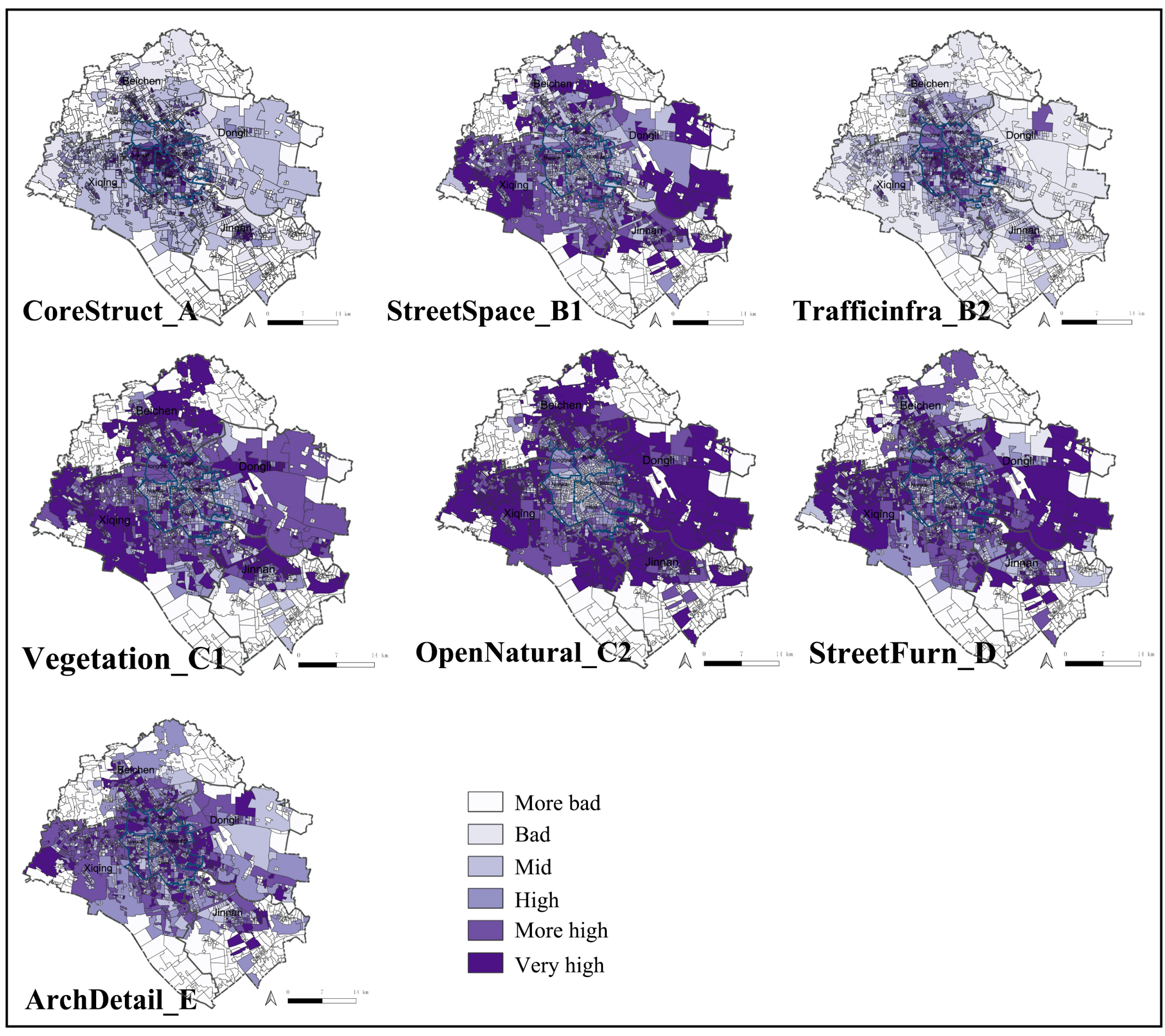
The spatial distribution of the seven objective street scene features (Figure 8) collectively shows a spatial gradient that follows a “compact-center, loose-periphery” pattern. The six central urban districts generally contain high-value clusters of core structures (CoreStruct_A), traffic flow (TrafficInfra_B2), street space (StreetSpace_B1), and architectural details (ArchDetail_E), particularly along the continuous belt spanning Heping, Nankai, and Hexi, as well as the corridor of the Hai River. These high-value zones correspond to areas of high-density building fabric, continuous street walls, historically significant architectural ensembles with rich facade details, and nodes of intense traffic activity. By contrast, the four suburban districts primarily exhibit high-value clusters of vegetation (Vegetation_C1) and open natural areas (OpenNatural_C2), which are extensively distributed along ecological corridors and in low-density residential areas. Street furniture (StreetFurn_D) reaches high values in localized areas along major thoroughfares and gateway nodes, while in most other areas it serves primarily functional rather than decorative roles. Core structures (CoreStruct_A) and traffic flow (TrafficInfra_B2) remain generally low in the periphery, with only localized high-value clusters emerging around district centers and transportation hubs.
Based on the correlations between subjective perceptions and spatial patterns, significant positive relationships were observed among the five perception dimensions overall (Figure 6b). In particular, the correlations between “enclosure–safety” ( r = 0.85 ), “human scale–complexity” ( r = 0.81 ), and “recognizability–safety” ( r = 0.82 ) are especially pronounced, suggesting that certain perceptions may be driven by similar spatial environmental factors [25]. By contrast, relatively weaker correlations, such as “complexity–recognizability,” suggest divergences in how these dimensions are understood. The strong interrelations between perception dimensions also expose blurred conceptual boundaries, highlighting the need for further theoretical refinement to reduce semantic ambiguity in subjective perception measurement. Figure 9 illustrates the spatial distribution of subjective perceptions across the study area. The six central urban districts exhibit high-value core zones across all five perceptual dimensions, whereas the four suburban districts display generally lower levels, with improvements only in specific new district centers, industrial parks, and recently developed residential areas. This differentiation closely aligns with the spatial patterns of objective features: the mature street networks, functional mix, and historical character of the central districts contribute to higher positive perceptions, while the low density, fragmented land uses, and diffuse boundaries of peripheral districts constrain perceptual improvements.

4.2. Spatial Hedonic Model Results

Figure 3a,c demonstrates the pronounced spatial clustering of housing prices. At both the apartment unit and community levels, prices follow a spatial gradient that declines with increasing distance from the Central Business District (CBD). Moran’s I reaches 0.78 ( p < 0.001 ), indicating strong positive spatial autocorrelation, with high- and low-priced residential areas clustering together. The LISA map (Figure 3d) further reveals that high-priced zones are concentrated within the inner ring and near the CBD, whereas low-priced areas are densely distributed beyond the outer ring.
In the spatial context outlined above, we first incorporate structural attributes, location attributes, and neighborhood attributes into the initial OLS regression model to construct the baseline model. The baseline model explains 54% of the price variation. Building on this, we further incorporate five types of subjective perception variables (Model 1) and seven types of objective street view feature indicators (Model 2) into the regression framework to examine their marginal effects in improving housing price modeling. Table 4 reports important regression diagnostic metrics. In terms of regression performance, Model 1 and Model 2 increase R 2 to 0.550 and 0.577, respectively, improving by 0.011 and 0.038 compared to the baseline model. This suggests that incorporating both subjective and objective street measures enhances the predictive power of the model. It shows that both types of street view indicators contribute to improving the model’s explanatory power, with a larger improvement from the objective features, consistent with findings from existing health and walkability studies [69]. It is worth noting that objective street features often correspond to visible/accessible exposure for commuters in corridors (e.g., StreetSpace_B1, TrafficInfra_B2, and Vegetation_C1), and the explanatory power gain they provide is linked to the impact of the surrounding environment on the experience of through-travelers, which also enters the price formation process.
To better capture this spatial non-stationarity and enhance prediction accuracy, this study applies the Geographical-XGBoost (G-XGBoost) model. Separate global models were constructed for the six urban districts and the four suburban districts, alongside both global and local models for the full study area. Table 5 reports their predictive performance. Among the global models, the urban model (Model 1) outperforms the suburban model (Model 0), with R 2 values of 0.710 and 0.598, respectively. The combined global model (Model 2) achieves an R 2 of 0.763, though with relatively high MAE and RMSE values. In contrast, the local model (Model 3), which employs an adaptive kernel to estimate each observation using the 177 nearest neighbors, fully reflects spatial heterogeneity. Its overall r 2 reaches 0.781, substantially surpassing all global models, underscoring the advantage of explicit spatial modeling for predictive performance.

4.3. Spatial Heterogeneity and Nonlinear Effects in Housing Price Drivers

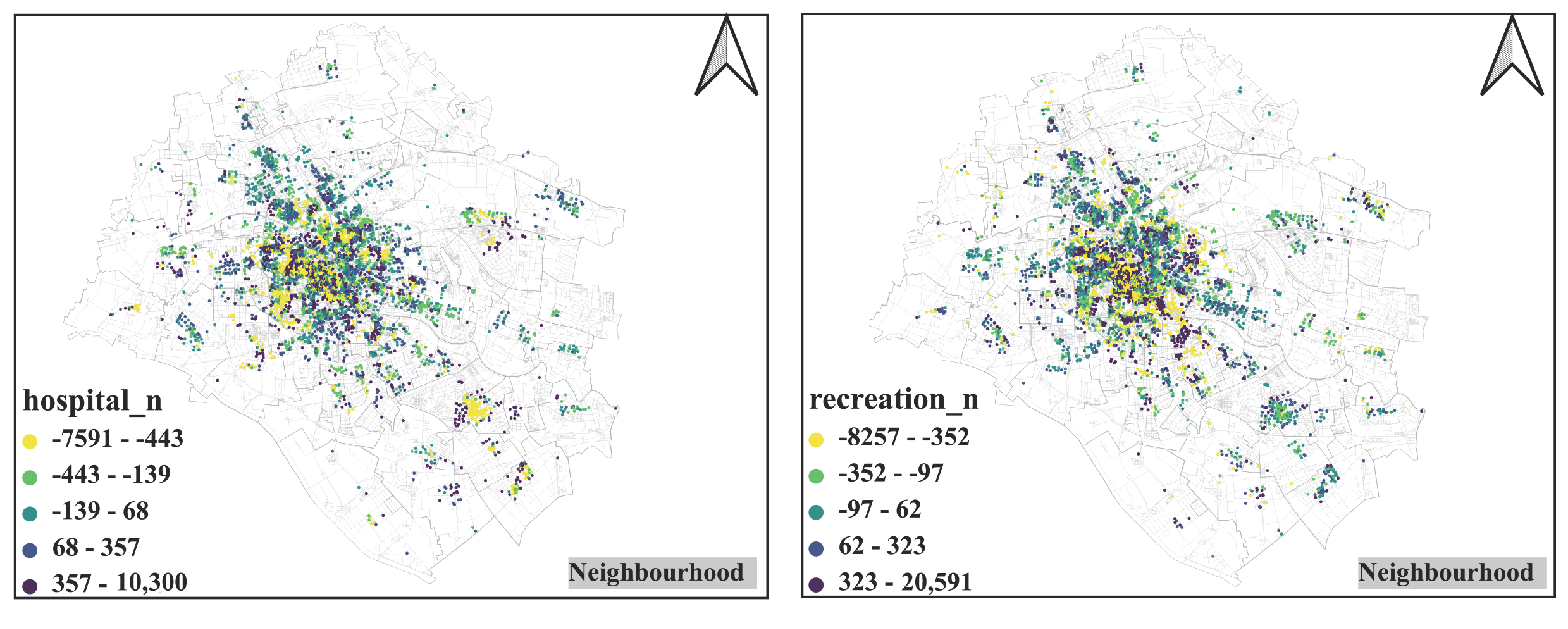
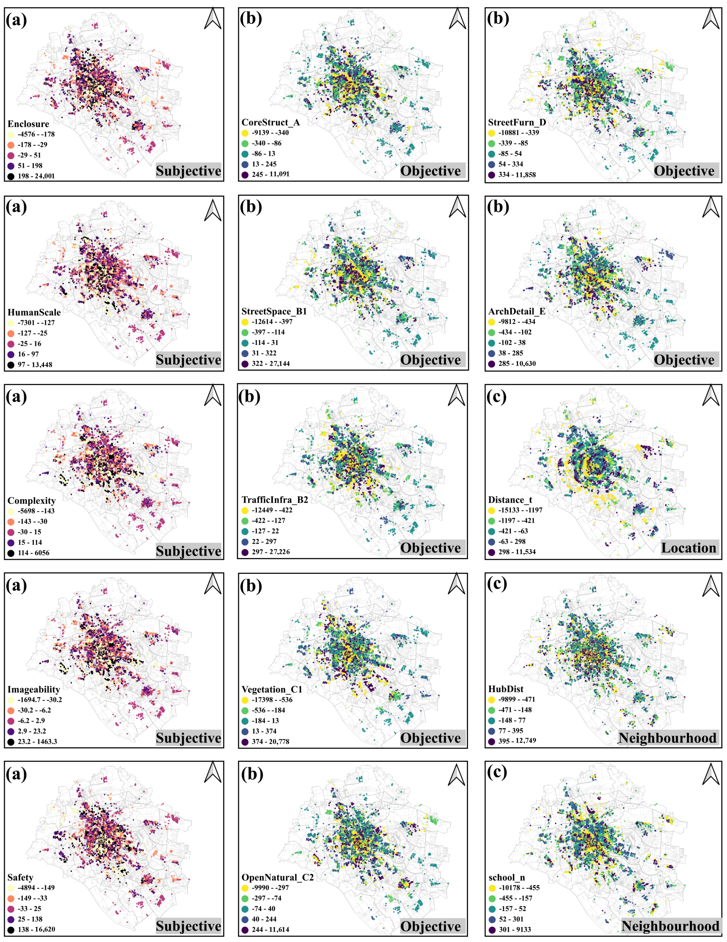
Given the significant spatial autocorrelation and non-stationarity of the OLS residuals, we further employ G-XGBoost for localized modeling and use SHAP metrics to spatially characterize the heterogeneity of price determinants. Figure 10 illustrates the spatial distribution of positive and negative local SHAP contributions of each variable to housing prices across the entire city. To facilitate understanding of the complex visualization, we divide the maps into four conceptual groups: Subjective, Objective, Location, and Neighborhood, and rank them according to SHAP values from high to low. All panels use a unified color scale (warm colors for positive, cool colors for negative). To ensure the readability of the visualization, the main text focuses on presenting the 15 “key variables,” covering four dimensions and forming a complementary information structure. The complete maps for other variables (Hospital_n, Recreation_n) are provided in the Appendix A Figure A1 for reference. Overall, for the Subjective dimension (Figure 10a), Enclosure, Complexity, Imageability, HumanScale, and Safety show larger positive patches in the core urban areas such as Heping, Nankai, and Hexi, while the positive patches in the peripheral areas are relatively scattered. In the Objective street view dimension (Figure 10b), Vegetation_C1 predominantly exhibits positive patches in most urban areas. StreetSpace_B1 and TrafficInfra_B2 show denser positive values around main roads and nearby nodes. CoreStruct_A, OpenNatural_C2, and ArchDetail_E appear with adjacent positive and negative patches in certain areas, indicating differences in the contribution direction across regions. In the Location and Neighborhood dimensions (Figure 10c), the spatial map of location attribute variables does not show a simple gradient trend of “the farther from the center, the lower the housing price.” The higher values of HubDist are mainly concentrated around several transportation nodes and their adjacent street segments, forming localized hotspot distributions. Positive hotspots for School_n are primarily found in the educational district clusters in the core urban areas. The maps in the Appendix A show that Hospital_n and Recreation_n exhibit larger positive patches in the peripheral areas. The larger positive patches appearing along the main corridors in the core urban areas can also be understood as the market’s spillover reflection of more traveler-friendly and safer continuous street segments for through-travelers. This spatial heterogeneity suggests that the same variable characteristics in different regions may have entirely different impacts and marginal effects on housing prices, reflecting the joint influence of social–spatial structures and market demand differences on housing prices.
To further investigate this heterogeneity, G-XGBoost global models were trained separately for the six urban and four suburban districts (see Table 5, Model 0, and Model 1). The SHAP summary plot visualizes each variable’s importance, direction, and impact distribution (Figure 11). Gray bars indicate the average contribution of each variable, with SHAP values on the X-axis representing positive or negative effects, and features sorted by importance on the Y-axis. Colors range from light yellow (low) to dark blue (high), reflecting feature magnitudes. Considerable differences in feature rankings between the urban districts (Figure 11b) and suburban districts (Figure 11a) suggest that homebuyers’ preferences vary markedly across regions.
Regarding neighborhood and location attributes, notable contrasts emerge. Educational resources dominate in the six urban districts, with School_n ranking first (average SHAP value 8203); its positive effects are concentrated in high-value samples, underscoring the importance of education in core areas. By contrast, hospitals (Hospital_n) rank lowest in the inner districts (SHAP values near zero), but third in the suburban districts, where they exert stronger positive effects, highlighting the role of medical access in peripheral housing markets. Commercial and recreational facilities (Recreation_n) rank mid-level (10th) in urban districts but rise to seventh in suburban districts, reflecting greater concern for lifestyle convenience among suburban buyers. The effect of distance to metro/bus stations (HubDist) shows spatial duality: in the urban core, dense transit networks limit its explanatory power, with SHAP values narrowly distributed (−2000 to 2000). In contrast, the distribution in suburban districts is wider (−3500 to 3000), indicating that transport accessibility remains important, though ranking slightly below medical and locational variables. This aligns with the daily commuting logic of through-travelers: in peripheral areas, marginal improvements in hub accessibility more directly affect inter-district travel costs and experiences, thereby reflecting in the price signals. Distance to the CBD (Distance_t) ranks second in the urban districts, confirming its strong influence there; in suburban districts, it remains stable as the dominant locational determinant.
For objective urban form and street scene characteristics, vegetation (Vegetation_C1) ranks among the top five in both the six inner districts and the four suburban districts, with average SHAP values of 4216 and 982, respectively. This shows that green coverage strongly boosts property prices across both regions. Within the inner districts, core structures (CoreStruct_A, average SHAP value 3845), architectural details (ArchDetail_E, 2982), and street furniture (StreetFurn_D, 2541) also rank highly, suggesting that homebuyers place greater emphasis on design aesthetics and the structural qualities of street spaces. These variables display a wide SHAP value range (approximately −5000 to 8000), with both positive and negative contributions. This pattern indicates a stratified response from homebuyers to design details, including a potential backlash from over-design. In the suburban districts, by contrast, the SHAP distributions for these indicators are more concentrated (approximately −2000 to 3000), showing a “passing grade” effect: once a certain threshold is met, a price premium is achieved, but additional improvements yield diminishing returns. In the inner districts, Complexity and Imageability rank fifth (average SHAP value 2316) and tenth (1245), respectively, indicating that perceived complexity and recognizability strongly affect property prices in the urban core. In the suburban districts, subjective perception variables rank lower overall, except for HumanScale. Safety ranks last (average SHAP value 86). This suggests that homebuyers and through-travelers in peripheral areas are less sensitive to street view design and perceptual quality, with the street view effect being more dependent on basic accessibility and functional conditions. Overall, street scene features in the inner districts play a differentiated and decisive role in shaping housing market outcomes, whereas, in the suburban districts, their influence is supplementary, acting mainly through infrastructure and transit accessibility.
To further explore the nonlinear variation characteristics and potential threshold effects within different value ranges, the SHAP dependence plot in Figure 12 is plotted based on the Geographical-XGBoost global model, as shown in Table 5, Model 2, systematically illustrating how subjective perception features, objective street view characteristics, and locational and neighborhood attributes contribute positively and negatively to housing prices at different value levels. This helps identify key turning points and nonlinear relationships at the global scale. In this study, all subjective perception variables exhibit pronounced nonlinear effects with clear thresholds (Figure 12a). Enclosure, HumanScale, and Safety show near-zero contributions in the low-value ranges (<0.6), with SHAP values fluctuating within ±2000 CNY/m2. Once the feature values reach approximately 0.66, 0.68, and 0.64, respectively, their contributions increase sharply (exceeding +8000 CNY/m2), reflecting the strong positive effect of improvements in enclosure, human scale, and safety on housing attractiveness. The enclosure, safety cues, and recognizability related to through-travelers exhibit stronger positive and threshold effects on public transportation corridors (e.g., limited impact below 0.60, with a significant enhancement in the 0.64–0.68 range). Notably, Enclosure reverses around 0.70, turning negative (about −4000 CNY/m2), possibly due to a sense of spatial oppression caused by excessive enclosure. Imageability and Complexity show negative effects in the low-value range (as low as −6000 CNY/m2), but rapidly shift to strong positive contributions (around +10,000 CNY/m2) after their respective thresholds, indicating that enhanced recognizability and design complexity can substantially increase housing desirability.
By contrast, objective street scene variables display more diverse threshold patterns (Figure 12b). CoreStruct_A is negative below 0.54 (–8000 CNY/m2) but rises steeply above this threshold to +12,000 CNY/m2, highlighting the strong positive correlation between building density and property prices. StreetSpace_B1 shows relatively modest effects overall (±2000 CNY/m2), whereas TrafficInfra_B2 exhibits steady positive growth in the mid-to-high range (up to +9000 CNY/m2), confirming the significant impact of improved transport accessibility. Vegetation_C1 maintains a consistently positive contribution across all ranges (+5000 to +7000 CNY/m2), underscoring the importance of urban greenery. In contrast, OpenNatural_C2 and ArchDetail_E shift from positive to negative at high values (down to −6000 CNY/m2), suggesting that excessive proportions of open sky, bare ground, or wall surfaces may reduce housing values, consistent with prior findings [17]. StreetFurn_D shows a marked positive effect in the low-to-mid range (+4000 to +6000 CNY/m2), after which the effect levels off.
Locational and neighborhood attributes (Figure 12c) also reveal strong nonlinear patterns. Distance to the CBD (Distance_t) has a clear threshold effect: within shorter distances (<7000 m), SHAP values remain above +10,000 CNY/m2, but around 7050 m, they shift sharply downward, becoming strongly negative (as low as −20,000 CNY/m2). Distance to the nearest metro or bus hub (HubDist), the number of hospitals within 1 km (Hospital_n), and the number of recreational/commercial facilities within 1 km (Recreation_n) all exhibit relatively small fluctuations (within ±2000 CNY/m2), suggesting that their marginal influence is limited once certain thresholds are met (approximately 142.42 m, 3 hospitals, and 13.88 facilities, respectively). By contrast, the number of schools within 1 km (School_n) shows a strong and sustained positive impact: SHAP values rise steadily with increasing school counts, from about +5000 CNY/m2 in the low range to +15,000 CNY/m2 at higher values, highlighting the crucial role of educational accessibility in driving housing prices. Compared to corridor-side street view features, HubDist, Hospital_n, and Recreation_n primarily reflect neighborhood and service accessibility, with limited direct relevance to through-travelers. In contrast, the significant and sustained positive effect of School_n aligns more closely with the quality of life dimension for residents (e.g., access to education and school commute convenience).

5. Discussion

5.1. The Impact of Street Design Quality on Property Prices

The adjusted R 2 values for OLS in Table 4 show that Model 2 ( R 2 = 0.577 ) improves by 2.7% compared to Model 1 ( R 2 = 0.550 ), with objective indicators explaining more variance overall than subjective indicators. This suggests that built environment factors have a stronger explanatory power for housing prices, which is consistent with the findings of Qiu et al. [26]. At the same time, OLS is constrained by the inherent limitations of global linearity and variable simplification [70]. In contrast, G-XGBoost captures nonlinear relationships and variable interactions within a unified framework and reveals the differences in feature importance across spatial units through local modeling. Previous studies also highlight its advantages in housing price prediction and mechanism interpretation [59]. In this study, Model 3 (local modeling of G-XGBoost) in Table 5 achieves an out-of-sample R 2 = 0.781 , outperforming all global models, while the spatial structure of the residuals is significantly reduced (see Table 4). This suggests that simultaneously incorporating nonlinearity and spatial heterogeneity within a unified framework is the key source of improved explanatory power, rather than simply model complexity [8].
For example, typical studies using the hedonic price model show that objective street view features (or more broadly, the built environment) often have stronger explanatory power compared to subjective perceptions [26], which is also confirmed by the OLS comparison in this study, as shown in Table 4. However, three common limitations of traditional approaches exist: first, in linear settings, non-monotonic relationships such as thresholds, platforms, and reversals, as well as higher-order interactions, are “linearized” and weakened; second, while GWR/SGWR relax spatial stationarity, they are still constrained by linear links and are unable to capture nonlinear margins and non-additive relationships [70]; third, introducing nonlinearity at the global level (tree models) while assuming spatial homogeneity makes it difficult to capture local preferences and facility endowment differences [8]. In the unified evidence framework of this study, these discrepancies are reformulated as two testable phenomena: G-XGBoost, through nonlinear marginal characterization (Figure 12), naturally reveals common reaction forms of street view elements, such as thresholds, platforms, and reversals (e.g., the insensitivity of Enclosure, HumanScale, and Safety in the low-value range, followed by gains after thresholds, and the “under-design” range turning negative for Imageability and Complexity); second, it outputs location-specific contribution distributions, visualizing the differences in the effects of the same feature across different locations and explaining the “same object, different effects”: in the core areas, complexity/recognizability over-design leads to marginal decline in the context of high density and functional mix, while in the peripheral areas, the “satisfactory” return occurs (benefits are gained once a threshold is reached, then decline afterward), accompanied by a shift in the dominance of the “accessibility–facility” channel (core areas benefiting more from educational accessibility, while peripheral areas expand in transport/medical accessibility), and a sensitivity distance shift to the CBD (Figure 11). These mechanized patterns align with the overall improvement in explanatory power observed in Table 5 and corroborate the conclusions on street view capitalization [26], the limitations of linear settings [70], and spatial effect heterogeneity [8].
The spatial consistency between subjective perceptions and objective street scene metrics (Figure 8, Figure 9 and Figure 10) indicates that the physical attributes of the built environment and residents’ visual experiences are closely intertwined in shaping housing prices. Nevertheless, this “form–perception” synergy varies significantly across locations. In central urban districts, high-value clusters of objective features such as core buildings (CoreStruct_A), traffic flow (TrafficInfra_B2), and street space (StreetSpace_B1) strongly overlap with perceptual dimensions such as enclosure, complexity, and imageability. This suggests that high-density, interconnected, and functionally mixed street forms simultaneously structure the physical environment and enhance residents’ perceptions [15,26]. By contrast, in peripheral districts, high-value clusters are more strongly associated with vegetation (Vegetation_C1) and open space features (OpenNatural_C2), corresponding to perceptions of safety (Safety) and human scale (HumanScale). This indicates that natural elements and open spaces are the primary drivers of positive perceptions in low-density areas [17]. These findings align with Xu’s [15] research, which showed that streets with clear spatial boundaries and diverse land uses are often associated with higher perception scores, and that such perceptions are significantly and positively correlated with housing prices.
The heterogeneous effects of subjective perceptions and objective street scenes on housing prices (Figure 11) demonstrate that the influence of environmental elements is strongly moderated by locational context and resident preferences. Street scene features that are scarce and desirable in central districts may lose their appeal in peripheral areas due to insufficient infrastructure or mismatched functions. For example, Yu [71] found in Wuhan that in peripheral areas, weak transportation and public services substantially diminish—and in some cases eliminate—the capitalization effect of landscape resources. Similarly, this study finds that green coverage yields a strong housing price premium in both regions, though with different magnitudes (4216 in inner districts and 982 in peripheral districts), consistent with prior research. Russell [72], for instance, found that in Baltimore, parks within half a mile generate a premium of 7.73–11.01%, while community-level open spaces yield premiums of about 5.93%.
This study finds that street design quality results in “over-design” in the core urban areas, while a “barely acceptable” effect is observed in the four surrounding districts. Hamidi [73] notes that “while the recognizability and transparency of streets can enhance property values, overly complex designs may have negative effects,” which provides theoretical support for the phenomenon of “over-design leading to negative SHAP values” observed in the core urban areas. This finding also aligns with research on how visibility and exposure influence risk perception and path choice, suggesting that in unfamiliar environments, increased interface complexity may raise information load and reduce predictability [20]. For different users, this mechanism is particularly relevant for through-travelers (pedestrians, cyclists, bus passengers, and drivers): they are less familiar with the street segments and rely more on clear interface cues and continuous sightlines for rapid recognition and path decision-making. In line with our SHAP spatial results, core corridors are more likely to exhibit negative contributions in the “complexity/recognizability” high-value range, indicating that information saturation and decreased predictability under travel exposure may pose adverse factors. Conversely, in peripheral corridors, nonlinear thresholds indicate that once basic human-scale, lighting, and coherent cycling network thresholds are met, marginal benefits are most significant, and further increases in decorative complexity yield limited additional benefits. These differences provide empirical evidence for “simplifying the interface information density of core corridors and improving the basic elements of peripheral corridors.”
This study reveals that the effect of most street view features on housing prices is not linearly increasing, but rather exhibits an optimal range and diminishing marginal effects, which is also reflected in existing studies [74]. On the subjective perception level, enclosure (Enclosure), human scale (HumanScale), and safety (Safety) have little significant impact on housing prices at low levels, but once key thresholds are reached, they bring about a noticeable price premium, reflecting the rigid demand of homebuyers for basic perceptual quality. Furthermore, street cues related to “enclosure” and “safety” not only benefit residents but may also improve the travel experience for through-travelers (such as bus passengers and electric bicycle riders) by reducing perceived risk and cognitive load. This conclusion aligns with existing studies on how street enclosure/safety and greenery enhance walking and cycling comfort [20,75]. Therefore, enclosure/safety can be considered priority design elements at the corridor level, with applicability across different user groups. However, excessive enclosure may cause a sense of spatial oppression, consistent with Hamidi’s (2020) conclusion that “excessive design complexity and recognizability can reduce livability” [73]. Similarly, imageability (Imageability) and complexity (Complexity) show negative effects at low levels, suggesting that inadequately designed street views may reduce market preference, with their positive effects only being realized once an appropriate threshold is reached. Among objective street features, the premium effect of core buildings (CoreStruct_A) is not significant when density is low, but once it exceeds a certain threshold, its positive impact on housing prices significantly increases. On the other hand, open natural spaces (OpenNatural_C2) and architectural details (ArchDetail_E) have a positive effect at moderate levels, but when their proportions are too high, they may lead to a decline in value due to a mismatch between function and demand. Notably, vegetation coverage (Vegetation_C1) maintains a stable premium effect across its entire range, consistent with a large body of empirical research on the capitalization effect of urban greenery [76], showing that its value is not constrained by a threshold.

5.2. The Intertwined Effects of Factors Influencing Housing Prices

In this study, the impact of educational resources on housing prices demonstrates a significant and robust premium effect, particularly in the core urban areas. The number of schools within a 1-kilometer radius (School_n) has an average SHAP value of 7800 in the central six districts, ranking first among all variables. Its positive contribution is concentrated in high-value samples, indicating that educational accessibility is the most competitive public resource in the central areas. This finding is consistent with studies in first-tier cities such as Beijing, Shanghai, and Shenzhen, suggesting that high-quality educational resources are highly capitalized due to the school district system, enrollment thresholds, and scarcity. Liu’s empirical study in Shanghai shows that a high-quality elementary school can bring about a 15.6% housing premium, directly quantifying the impact of education capitalization [77]; Zhou [78] further points out that school district premiums in Beijing and Shanghai are approximately 8.1% and 6.5%, respectively, highlighting the significant value of educational resources in first-tier cities and emphasizing the powerful driving effect of educational resources on housing prices in core areas. This indicates that this capitalization mechanism is not limited to traditional first-tier cities like Beijing, Shanghai, and Guangzhou, but is also applicable to rapidly developing emerging metropolises. In the central six districts, this premium effect not only reflects the rigid demand for high-quality education from homebuyers but is also amplified by the concentration of high-income families and families with school-aged children, further increasing the price elasticity of educational resources. It is noteworthy that, unlike the “enclosure” and “safety” cues discussed earlier (which can simultaneously improve the immediate commuting experience for both residents and through-travelers along commuting corridors), educational accessibility primarily affects the long-term quality of life and school district choice for residents, with a weaker association with through-travelers. Therefore, we interpret the findings related to schools as a resident-oriented benefit channel, while enclosure and safety are considered corridor-level channels that apply across different population groups. Together, they form complementary “long-term—short-term” pathways [79]. In contrast, in the peripheral four districts, the importance of School_n significantly decreases, and the overall supply of educational resources is insufficient, with considerable quality variation. As a result, an increase in the number of schools does not necessarily lead to an improvement in quality. At the same time, homebuyers’ decisions in the peripheral areas are more dependent on transportation accessibility, healthcare facilities, and commercial convenience, with educational accessibility relatively lower in the decision-making priority. This finding is consistent with Liu [80] in Wuhan, which indicates that in peripheral areas with inadequate transportation and public services, the capitalization effect of educational resources significantly weakens or even disappears.
Beyond education, this study also reveals the “dual natur” of transportation accessibility, locational factors, medical facilities, and commercial/recreational amenities. In the six urban districts, where subway, bus, and medical resources are already saturated, the marginal contributions of HubDist and Hospital_n to housing prices are limited, as reflected by narrow SHAP fluctuations. In contrast, in the four suburban districts, their influence expands considerably. This finding aligns with Jin’s research in Beijing [81], which shows that in core areas with abundant transit and healthcare resources, these accessibility indicators have limited explanatory power for price variation, whereas in peripheral areas with weaker infrastructure, transportation and healthcare accessibility become primary drivers of housing premiums. In the six inner districts, housing prices also show very high sensitivity to distance from the CBD, ranking second in SHAP values, and decline significantly with increasing distance. This result is consistent with the classic Bid-Rent Theory, which posits that proximity to the city center drives higher land values [82]. Empirically, Chen and Hao’s analysis of new residential data in Shanghai confirms that housing prices decline as distance from the CBD increases, underscoring that locational advantage in core areas remains a fundamental driver of housing price formation [11].
Taken together, housing prices are shaped by the interplay of locational advantages, public service provision, and street scene quality. In core areas, educational resources, proximity to the CBD, and high-quality street environments often co-occur, creating a “bundling premium effect.” By contrast, in peripheral areas, weak infrastructure such as limited transit and healthcare may diminish—or even reverse—the positive impact of features like green space and open areas. This interdependence helps explain why certain street scene variables shift from positive to negative contributions across regions, reflecting the moderating influence of market demand and functional matching on the housing price effect.

5.3. Implications for Urban Planning

This study provides an evidence-based foundation for urban planning from a morphological perspective, suggesting that planning and design should integrate the comprehensive effects of street environments, building quality, and surrounding facilities. These factors not only influence housing prices and residents’ livability but are also closely related to urban sustainability. Furthermore, streets have cross-community passage attributes: public transit passengers, cyclists, and through-traffic from other neighborhoods also use these streets. Therefore, “corridor-side” cues such as enclosure and safety (continuous street walls, transparent interfaces, clear sightlines, lighting, facade maintenance, and tree cover) not only enhance residents’ experience but also immediately improve the comfort and safety of through-travelers, thus expanding the beneficiaries from homebuyers and residents to a broader population. In terms of public service and opportunity distribution, efforts should be made to promote balanced educational resources between the core and peripheral areas: in peripheral areas, high-quality schools should be added, and transportation and public services should be improved to enhance residential attractiveness. At the same time, attention should be paid to the over-capitalization of school district systems. By optimizing school district planning and promoting educational equity, it is important to avoid long-term price distortions and spatial inequality caused by resource monopolies.
This study identifies the “over-design” effect in street views within the core areas and the “minimal” effect in the suburban areas. This finding suggests that urban design should adopt differentiated strategies based on location: in core areas, the focus should be on functional integration and moderate design complexity to avoid negative perceptions caused by excessive decoration or high density; in suburban areas, priority should be given to ensuring the basic quality and functionality of street views, providing residents with a fundamental livable experience, and enhancing attractiveness through appropriate greening and open space configurations. For policymakers, this means that urban landscape optimization should establish a “best design range” based on location characteristics to achieve a win-win scenario for both real estate value and residents’ perceptions.This study comprehensively compares the influence of subjective perceptions, objective street indicators, neighborhood attributes, and location on housing prices, revealing their intertwined roles and practical significance in urban planning. It provides valuable reference for real estate developers, policymakers, researchers, and urban planners. While subjective street perceptions and objective street indices are not the ultimate determinants of housing prices, they significantly influence them. Therefore, governments and decision-makers should prioritize the design of street quality surrounding residential areas, particularly within a 15 min walking radius, to enhance both the functionality and perceived quality of street environments, thereby improving residents’ quality of life and satisfaction with their living conditions.
The results of this study provide researchers with a more comprehensive understanding when analyzing urban heterogeneity patterns, helping to reveal the differences in housing price determinants between cities. Researchers can more accurately identify the conditions necessary for different housing price levels, providing theoretical support for further urban housing price studies and policy formulation. For policymakers, this means setting the “optimal design range” based on location characteristics: prioritizing passage experience and safety in street corridors, and prioritizing long-term quality of life and public services in neighborhood areas, thereby achieving dual benefits of “immediate-long-term, cross-group-resident” effects. It is recommended to establish regular impact assessments (such as travel perception and satisfaction, cycling/walking usage rates and accident rates, public transit waiting experience index, education accessibility and enrollment opportunity indicators) to support design iteration and policy optimization in a closed loop. Finally, this study reveals new directions for street design guidelines, particularly through the integrated analysis of subjective perception scores and objective environmental features. Urban designers and planners can more deeply examine individual perceptions of street environments, thereby providing guidance for sustainable public transportation infrastructure planning, urban micro-renovation, and vibrant, safe neighborhood design. By integrating these factors, urban design can not only better cater to homebuyers’ preferences but also enhance residents’ quality of life, promoting sustainable urban development.

5.4. Limitations and Potential Improvements

This study still has several limitations that need to be addressed in future work. First, the analysis is based on correlation identification, and does not directly infer causal relationships. This is because there may be bidirectional causality between housing prices and street environments, or overlooked confounding factors (e.g., infrastructure investment policies). Future research could incorporate methods such as instrumental variables and natural experiments to enhance causal inference capabilities. The study is based on a case study of Tianjin, and while it reveals the differences in the importance of housing price determinants across different geographic areas, urban spatial heterogeneity is often more complex and may be influenced by multiple factors such as historical, cultural, and policy backgrounds. Therefore, a cross-city comparison should be conducted to validate the robustness and generalizability of the conclusions.
Second, the perceptual evaluators mainly come from professional backgrounds such as architecture, planning, and landscape design, and thus do not fully encompass the perspectives of potential homebuyers. Moreover, the limitations of the current online platform restricted the consistency check among evaluators. In the future, the evaluator pool should be expanded and the crowdsourcing platform design optimized to improve data representativeness and reliability.
Third, while this study includes the number of schools within a 1000 m radius around residential points (school_n) as a neighborhood attribute, and the results show its significant positive impact on housing prices in the central districts, it does not fully address the complexity of the concept of “school district housing” in Tianjin. It fails to reflect the complexity of school district boundaries, school hierarchy, and enrollment policies, which may have oversimplified the premium mechanism of school district housing. Future research could incorporate administrative data on school districts and school quality indicators to more precisely capture the role of educational resources in housing prices.
Finally, while the Geographical-XGBoost algorithm, as the core analytical tool of this study, performs excellently in capturing spatial heterogeneity and nonlinear relationships, it also has some limitations. On one hand, the construction of local models in Geographical-XGBoost depends on spatial kernel functions, and the neighborhood parameters (such as the k-value or bandwidth) are usually optimized through cross-validation methods. However, the choice of bandwidth can still be influenced by data characteristics and the parameter range, which may impact the stability and generalizability of the results. On the other hand, large-scale geographic data processing incurs high computational costs and relies heavily on high-quality training data and feature engineering. Future research could explore better-supported weight functions and adaptive parameter selection mechanisms, introduce high-performance computing to improve operational efficiency, and integrate automated feature selection and dimensionality reduction methods to enhance model robustness and interpretability, thereby further expanding its application potential in urban spatial modeling.

6. Conclusions

This study integrates subjective street perception, objective visual elements, and neighborhood–location attributes into the Geographical-XGBoost framework, which accounts for both nonlinearity and spatial heterogeneity. It systematically compares the comprehensive impact of street design quality and socio-economic factors on housing prices in Tianjin, and examines the differences in the importance and interplay of housing price determinants across different geographical spaces. Compared to the traditional Hedonic Pricing Model (HPM), the inclusion of both subjective and objective street view information significantly enhances explanatory power and transforms the concept of a “good street” from a conceptual judgment into quantifiable design clues, such as the effective ranges and marginal effects of enclosure, safety, human scale, and recognizability.
The results of this study indicate that most street environment variables have a positive relationship with housing prices, which aligns with the preferences of Chinese homebuyers for good street landscapes, pleasant scales, and open spaces [83], emphasizing the importance of considering street environment quality in housing value assessments. Enclosure, human scale, and safety contribute nearly zero to housing prices at low levels, but show significant gains once a threshold is surpassed, with excessive enclosure potentially leading to negative effects. These findings point towards the “moderately optimal” design principle. On top of this mechanism, a clear core–periphery contrast emerges spatially: the core area often features the co-occurrence of “core buildings, street space, and transportation infrastructure” with “complexity and recognizability,” while the peripheral area primarily couples “greening, open spaces, safety, and human scale.” Further, the over-design of “complexity and recognizability” in the core area is more likely to impose recognition burdens and path uncertainty on through-travelers (pedestrians, cyclists, bus passengers, and drivers), while residents, due to their familiarity, are less sensitive to these factors. This difference explains the divergent effects of the same design on different users. Therefore, in practical terms, differentiated “corridor–district” implementation pathways can be established based on these insights. Specifically, for commuter corridors, cross-group, immediate benefits can be achieved through street interface continuity and visible safety elements. These elements not only improve the walking and stopping experience for residents but also immediately reduce the perceived risk and cognitive load for through-travelers. For residential districts, long-term benefits primarily depend on school accessibility and the balanced provision of community public services, which should be enhanced in peripheral areas through improved accessibility and equitable distribution mechanisms to avoid spatial inequality resulting from the over-capitalization of educational resources.
In summary, this study not only provides empirical evidence but also translates the impact of “street view—neighborhood—location” on housing values into actionable urban design and governance pathways. Future research could verify the robustness of thresholds and spatial heterogeneity across multiple cities and contexts, combining instrumental variables or natural experiments to strengthen causal identification, and further refine the implementation of Geographical-XGBoost in neighborhood adaptation and model interpretation. Additionally, it is recommended to establish regular monitoring indicators, such as travel perception and satisfaction, walking and cycling usage rates and accident rates, bus passenger waiting experience index, and educational accessibility and enrollment opportunity indicators, to support rolling evaluations and policy optimization.

Author Contributions

Conceptualization, Shengbei Zhou, Qian Ji, Pengbo Li and Jun Wu; data curation, Shengbei Zhou and Yuqiao Zhang; formal analysis, Shengbei Zhou, Pengbo Li and Longhao Zhang; funding acquisition, Qian Ji; investigation, Shengbei Zhou, Longhao Zhang, Pengbo Li and Yuqiao Zhang; methodology, Shengbei Zhou and Qian Ji; project administration, Qian Ji; resources, Pengbo Li and Jun Wu; software, Shengbei Zhou and Qian Ji; supervision, Qian Ji, Jun Wu and Pengbo Li; validation, Shengbei Zhou, Qian Ji and Yuqiao Zhang; visualization, Shengbei Zhou, Pengbo Li, Jun Wu and Longhao Zhang; writing—original draft, Shengbei Zhou and Qian Ji; writing—review and editing, Qian Ji, Jun Wu, Longhao Zhang and Pengbo Li. All authors have read and agreed to the published version of the manuscript.

Funding

This research was funded by the Tianjin Art Science Planning General Project, project number A22039.

Data Availability Statement

The original contributions presented in the study are included in the article; further inquiries can be directed to the corresponding author.

Conflicts of Interest

The authors declare that they have no known competing financial interests or personal relationships that could have appeared to influence the work reported in this paper.

Appendix A

Figure A1. Neighborhood Attributes: Local G-XGBoost shape value; space distribution; medical and commercial entertainment facilities.SHAP values are sorted in descending order. Warm colors indicate positive contributions, while cool colors indicate negative contributions.
Ijgi 14 00391 g0a1

References

  1. WHO. Air Pollution and Child Health: Prescribing Clean Air; World Health Organization: Geneva, Switzerland, 2018. [Google Scholar]
  2. Liu, R.; Li, T.; Greene, R. Migration and Inequality in Rental Housing: Affordability Stress in the Chinese Cities. Appl. Geogr. 2020, 115, 102138. [Google Scholar] [CrossRef]
  3. Geng, B.; Bao, H.; Liang, Y. A Study of the Effect of a High-Speed Rail Station on Spatial Variations in Housing Price Based on the Hedonic Model. Habitat Int. 2015, 49, 333–339. [Google Scholar] [CrossRef]
  4. Li, Y.; Lin, Y.; Wang, J.; Geertman, S.; Hooimeijer, P. The effects of jobs, amenities, and locations on housing submarkets in Xiamen City, China. J. Hous. Built Environ. 2023, 38, 1221–1239. [Google Scholar] [CrossRef]
  5. Köberl, M.; Wurm, M.; Droin, A.; Garbasevschi, O.M.; Dolls, M.; Taubenböck, H. Liveability in Large Housing Estates in Germany—Identifying Differences Based on a Novel Concept for a Walkable City. Landsc. Urban Plan. 2024, 251, 105150. [Google Scholar] [CrossRef]
  6. Xu, Y.; Chen, R.; Du, H.; Chen, M.; Fu, C.; Li, Y. Evaluation of green space influence on housing prices using machine learning and urban visual intelligence. Cities 2025, 158, 105661. [Google Scholar] [CrossRef]
  7. Xu, Y.; Wang, L. GIS-based analysis of obesity and the built environment in the US. Cartogr. Geogr. Inf. Sci. 2015, 42, 9–21. [Google Scholar] [CrossRef]
  8. Zhu, J.; Gong, Y.; Liu, C.; Du, J.; Song, C.; Chen, J.; Pei, T. Assessing the Effects of Subjective and Objective Measures on Housing Prices with Street View Imagery: A Case Study of Suzhou. Land 2023, 12, 2095. [Google Scholar] [CrossRef]
  9. Liu, N.; Strobl, J. Impact of Neighborhood Features on Housing Resale Prices in Zhuhai (China) Based on an (M)GWR Model. Big Earth Data 2023, 7, 146–169. [Google Scholar] [CrossRef]
  10. Wen, H.; Tao, Y. Polycentric Urban Structure and Housing Price in the Transitional China: Evidence from Hangzhou. Habitat Int. 2015, 46, 138–146. [Google Scholar] [CrossRef]
  11. Chen, J.; Hao, Q. The Impacts of Distance to CBD on Housing Prices in Shanghai: A Hedonic Analysis. J. Chin. Econ. Bus. Stud. 2008, 6, 291–302. [Google Scholar] [CrossRef]
  12. Liang, X.; Liu, Y.; Qiu, T.; Jing, Y.; Fang, F. The Effects of Locational Factors on the Housing Prices of Residential Communities: The Case of Ningbo, China. Habitat Int. 2018, 81, 1–11. [Google Scholar] [CrossRef]
  13. Wen, H.; Zhang, Y.; Zhang, L. Do Educational Facilities Affect Housing Price? An Empirical Study in Hangzhou, China. Habitat Int. 2014, 42, 155–163. [Google Scholar] [CrossRef]
  14. Qiu, W.; Li, W.; Liu, X.; Zhang, Z.; Li, X.; Huang, X. Subjective and Objective Measures of Streetscape Perceptions: Relationships with Property Value in Shanghai. Cities 2023, 132, 104037. [Google Scholar] [CrossRef]
  15. Xu, X.; Qiu, W.; Li, W.; Liu, X.; Zhang, Z.; Li, X.; Luo, D. Associations between Street-View Perceptions and Housing Prices: Subjective vs. Objective Measures Using Computer Vision and Machine Learning Techniques. Remote Sens. 2022, 14, 891. [Google Scholar] [CrossRef]
  16. Ewing, R.H.; Clemente, O.; Neckerman, K.M.; Purciel-Hill, M.; Quinn, J.W.; Rundle, A. Measuring Urban Design: Metrics for Livable Places; Island Press: Washington, DC, USA, 2013; Volume 200. [Google Scholar]
  17. Ma, X.; Ma, C.; Wu, C.; Xi, Y.; Yang, R.; Peng, N.; Zhang, C.; Ren, F. Measuring human perceptions of streetscapes to better inform urban renewal: A perspective of scene semantic parsing. Cities 2021, 110, 103086. [Google Scholar] [CrossRef]
  18. Cheng, J.; Zhang, X.; Huang, J. Optimizing the spatial scale for neighborhood environment characteristics using fine-grained data. Int. J. Appl. Earth Obs. Geoinf. 2022, 106, 102659. [Google Scholar] [CrossRef]
  19. Sander, H.; Polasky, S.; Haight, R.G. The value of urban tree cover: A hedonic property price model in Ramsey and Dakota Counties, Minnesota, USA. Ecol. Econ. 2010, 69, 1646–1656. [Google Scholar] [CrossRef]
  20. Campos Ferreira, M.; Dias Costa, P.; Abrantes, D.; Hora, J.; Felício, S.; Coimbra, M.; Galvão Dias, T. Identifying the determinants and understanding their effect on the perception of safety, security, and comfort by pedestrians and cyclists: A systematic review. Transp. Res. Part Traffic Psychol. Behav. 2022, 91, 136–163. [Google Scholar] [CrossRef]
  21. Hamim, O.F.; Ukkusuri, S.V. Towards safer streets: A framework for unveiling pedestrians’ perceived road safety using street view imagery. Accid. Anal. Prev. 2024, 195, 107400. [Google Scholar] [CrossRef] [PubMed]
  22. Li, X.; Zhang, C.; Li, W.; Ricard, R.; Meng, Q.; Zhang, W. Assessing street-level urban greenery using Google Street View and a modified green view index. Urban For. Urban Green. 2015, 14, 675–685. [Google Scholar] [CrossRef]
  23. Yin, L.; Wang, Z. Measuring visual enclosure for street walkability: Using machine learning algorithms and Google Street View imagery. Appl. Geogr. 2016, 76, 147–153. [Google Scholar] [CrossRef]
  24. Zhou, H.; He, S.; Cai, Y.; Wang, M.; Su, S. Social inequalities in neighborhood visual walkability: Using street view imagery and deep learning technologies to facilitate healthy city planning. Sustain. Cities Soc. 2019, 50, 101605. [Google Scholar] [CrossRef]
  25. Ewing, R.; Handy, S. Measuring the Unmeasurable: Urban Design Qualities Related to Walkability. J. Urban Des. 2009, 14, 65–84. [Google Scholar] [CrossRef]
  26. Qiu, W.; Zhang, Z.; Liu, X.; Li, W.; Li, X.; Xu, X.; Huang, X. Subjective or objective measures of street environment, which are more effective in explaining housing prices? Landsc. Urban Plan. 2022, 221, 104358. [Google Scholar] [CrossRef]
  27. Despotovic, M.; Koch, D.; Thaler, S.; Stumpe, E.; Brunauer, W.; Zeppelzauer, M. Linking repeated subjective judgments and ConvNets for multimodal assessment of the immediate living environment. MethodsX 2024, 12, 102556. [Google Scholar] [CrossRef]
  28. Tang, Y.; Xiao, W.; Yuan, F. Evaluating objective and perceived ecosystem service in urban context: An indirect method based on housing market. Landsc. Urban Plan. 2025, 254, 105245. [Google Scholar] [CrossRef]
  29. Dubey, A.; Naik, N.; Parikh, D.; Raskar, R.; Hidalgo, C.A. Deep Learning the City: Quantifying Urban Perception at a Global Scale. In Proceedings of the Computer Vision—ECCV 2016, Amsterdam, The Netherlands, 11–14 October 2016; Leibe, B., Matas, J., Sebe, N., Welling, M., Eds.; Springer: Cham, Switzerland, 2016; pp. 196–212. [Google Scholar] [CrossRef]
  30. Kang, Y.; Zhang, F.; Gao, S.; Peng, W.; Ratti, C. Human settlement value assessment from a place perspective: Considering human dynamics and perceptions in house price modeling. Cities 2021, 118, 103333. [Google Scholar] [CrossRef]
  31. Sun, M.; Zhang, F.; Duarte, F.; Ratti, C. Understanding architecture age and style through deep learning. Cities 2022, 128, 103787. [Google Scholar] [CrossRef]
  32. Rosen, S. Hedonic Prices and Implicit Markets: Product Differentiation in Pure Competition. J. Political Econ. 1974, 82, 34–55. [Google Scholar] [CrossRef]
  33. Su, S.; Zhang, J.; He, S.; Zhang, H.; Hu, L.; Kang, M. Unraveling the impact of TOD on housing rental prices and implications on spatial planning: A comparative analysis of five Chinese megacities. Habitat Int. 2021, 107, 102309. [Google Scholar] [CrossRef]
  34. Wu, C.; Ye, X.; Du, Q.; Luo, P. Spatial effects of accessibility to parks on housing prices in Shenzhen, China. Habitat Int. 2017, 63, 45–54. [Google Scholar] [CrossRef]
  35. Wan, H.; Chowdhury, P.K.R.; Yoon, J.; Bhaduri, P.; Srikrishnan, V.; Judi, D.; Daniel, B. Explaining drivers of housing prices with nonlinear hedonic regressions. Mach. Learn. Appl. 2025, 21, 100707. [Google Scholar] [CrossRef]
  36. McCord, M.; McCord, J.; Lo, D.; Brown, L.; MacIntyre, S.; Squires, G. The value of green and blue space: Walkability and house prices. Cities 2024, 154, 105377. [Google Scholar] [CrossRef]
  37. Ye, Y.; Xie, H.; Fang, J.; Jiang, H.; Wang, D. Daily Accessed Street Greenery and Housing Price: Measuring Economic Performance of Human-Scale Streetscapes via New Urban Data. Sustainability 2019, 11, 1741. [Google Scholar] [CrossRef]
  38. Chen, L.; Yao, X.; Liu, Y.; Zhu, Y.; Chen, W.; Zhao, X.; Chi, T. Measuring Impacts of Urban Environmental Elements on Housing Prices Based on Multisource Data—A Case Study of Shanghai, China. ISPRS Int. J.-Geo-Inf. 2020, 9, 106. [Google Scholar] [CrossRef]
  39. Tang, C.K.; Le, T. Crime risk and housing values: Evidence from the gun offender registry. J. Urban Econ. 2023, 134, 103526. [Google Scholar] [CrossRef]
  40. Shen, Y.; Karacsonyi, D. Assessing the urban–rural fringe using gradient and patch metrics in Tianjin, China. J. Geogr. Syst. 2022, 24, 77–98. [Google Scholar] [CrossRef]
  41. Gao, C.; Feng, Y.; Tong, X.; Lei, Z.; Chen, S.; Zhai, S. Modeling urban growth using spatially heterogeneous cellular automata models: Comparison of spatial lag, spatial error and GWR. Comput. Environ. Urban Syst. 2020, 81, 101459. [Google Scholar] [CrossRef]
  42. Gao, Y.; Zhao, J.; Han, L. Exploring the spatial heterogeneity of urban heat island effect and its relationship to block morphology with the geographically weighted regression model. Sustain. Cities Soc. 2022, 76, 103431. [Google Scholar] [CrossRef]
  43. Xie, Y.; Nhu, A.N.; Song, X.P.; Jia, X.; Skakun, S.; Li, H.; Wang, Z. Accounting for spatial variability with geo-aware random forest: A case study for US major crop mapping. Remote Sens. Environ. 2025, 319, 114585. [Google Scholar] [CrossRef]
  44. Ye, M.; Zhu, L.; Li, X.; Ke, Y.; Huang, Y.; Chen, B.; Yu, H.; Li, H.; Feng, H. Estimation of the soil arsenic concentration using a geographically weighted XGBoost model based on hyperspectral data. Sci. Total Environ. 2023, 858, 159798. [Google Scholar] [CrossRef] [PubMed]
  45. Ouyang, L.; Yang, Y.; Wu, Z.; Jiang, Q.; Qiao, R. Towards inclusive urbanism: An examination of urban environment strategies for enhancing social equity in Chengdu’s housing zones. Sustain. Cities Soc. 2024, 107, 105414. [Google Scholar] [CrossRef]
  46. Ge, J. Endogenous rise and collapse of housing price: An agent-based model of the housing market. Comput. Environ. Urban Syst. 2017, 62, 182–198. [Google Scholar] [CrossRef]
  47. Park, H.; Lee, S.; Lee, J.; Ham, B. Learning by Aligning: Visible-Infrared Person Re-identification using Cross-Modal Correspondences. In Proceedings of the 2021 IEEE/CVF International Conference on Computer Vision (ICCV), Montreal, QC, Canada, 11–17 October 2021; pp. 12026–12035. [Google Scholar] [CrossRef]
  48. Gibril, M.B.A.; Al-Ruzouq, R.; Shanableh, A.; Jena, R.; Bolcek, J.; Shafri, H.Z.M.; Ghorbanzadeh, O. Transformer-based semantic segmentation for large-scale building footprint extraction from very-high resolution satellite images. Adv. Space Res. 2024, 73, 4937–4954. [Google Scholar] [CrossRef]
  49. Gu, Y.; Fu, C.; Song, W.; Wang, X.; Chen, J. RTLinearFormer: Semantic segmentation with lightweight linear attentions. Neurocomputing 2025, 625, 129489. [Google Scholar] [CrossRef]
  50. Zhou, B.; Zhao, H.; Puig, X.; Fidler, S.; Barriuso, A.; Torralba, A. Scene Parsing Through ADE20K Dataset. In Proceedings of the IEEE Conference on Computer Vision and Pattern Recognition (CVPR), Honolulu, HI, USA, 21–26 July 2017. [Google Scholar]
  51. Gehl, J. Cities for People; Island Press: Washington, DC, USA, 2010. [Google Scholar]
  52. Naik, N.; Philipoom, J.; Raskar, R.; Hidalgo, C. Streetscore—Predicting the Perceived Safety of One Million Streetscapes. In Proceedings of the 2014 IEEE Conference on Computer Vision and Pattern Recognition Workshops, Columbus, OH, USA, 23–28 July 2014; pp. 793–799. [Google Scholar] [CrossRef]
  53. He, L.; Páez, A.; Liu, D. Built environment and violent crime: An environmental audit approach using Google Street View. Comput. Environ. Urban Syst. 2017, 66, 83–95. [Google Scholar] [CrossRef]
  54. Salesses, P.; Schechtner, K.; Hidalgo, C.A. The Collaborative Image of The City: Mapping the Inequality of Urban Perception. PLoS ONE 2013, 8, e68400. [Google Scholar] [CrossRef]
  55. Verma, D.; Jana, A.; Ramamritham, K. Predicting human perception of the urban environment in a spatiotemporal urban setting using locally acquired street view images and audio clips. Build. Environ. 2020, 186, 107340. [Google Scholar] [CrossRef]
  56. Ito, K.; Biljecki, F. Assessing bikeability with street view imagery and computer vision. Transp. Res. Part C Emerg. Technol. 2021, 132, 103371. [Google Scholar] [CrossRef]
  57. Huang, Z.; Chen, R.; Xu, D.; Zhou, W. Spatial and hedonic analysis of housing prices in Shanghai. Habitat Int. 2017, 67, 69–78. [Google Scholar] [CrossRef]
  58. Kutner, M.H.; Nachtsheim, C.J.; Neter, J. Applied Linear Regression Models, 4th ed.; McGraw-Hill/Irwin: Columbus, OH, USA, 2004. [Google Scholar]
  59. Grekousis, G. Geographical-XGBoost: A New Ensemble Model for Spatially Local Regression Based on Gradient-Boosted Trees. J. Geogr. Syst. 2025, 27, 169–195. [Google Scholar] [CrossRef]
  60. Li, Y.; Zhang, Y.; Wu, Q.; Xue, R.; Wang, X.; Si, M.; Zhang, Y. Greening the concrete jungle: Unveiling the co-mitigation of greenspace configuration on PM2.5 and land surface temperature with explanatory machine learning. Urban For. Urban Green. 2023, 88, 128086. [Google Scholar] [CrossRef]
  61. Beleites, C.; Neugebauer, U.; Bocklitz, T.; Krafft, C.; Popp, J. Sample Size Planning for Classification Models. Anal. Chim. Acta 2013, 760, 25–33. [Google Scholar] [CrossRef] [PubMed]
  62. Niu, T.; Chen, Y.; Yuan, Y. Measuring urban poverty using multi-source data and a random forest algorithm: A case study in Guangzhou. Sustain. Cities Soc. 2020, 54, 102014. [Google Scholar] [CrossRef]
  63. Yao, Y.; Liang, Z.; Yuan, Z.; Liu, P.; Bie, Y.; Zhang, J.; Wang, R.; Wang, J.; Guan, Q. A human-machine adversarial scoring framework for urban perception assessment using street-view images. Int. J. Geogr. Inf. Sci. 2019, 33, 2363–2384. [Google Scholar] [CrossRef]
  64. Roy, K.; Das, R.N.; Ambure, P.; Aher, R.B. Be aware of error measures. Further studies on validation of predictive QSAR models. Chemom. Intell. Lab. Syst. 2016, 152, 18–33. [Google Scholar] [CrossRef]
  65. Zhang, F.; Zhou, B.; Liu, L.; Liu, Y.; Fung, H.H.; Lin, H.; Ratti, C. Measuring human perceptions of a large-scale urban region using machine learning. Landsc. Urban Plan. 2018, 180, 148–160. [Google Scholar] [CrossRef]
  66. Griew, P.; Hillsdon, M.; Foster, C.; Coombes, E.; Jones, A.; Wilkinson, P. Developing and testing a street audit tool using Google Street View to measure environmental supportiveness for physical activity. Int. J. Behav. Nutr. Phys. Act. 2013, 10, 103. [Google Scholar] [CrossRef]
  67. Rundle, A.G.; Bader, M.D.; Richards, C.A.; Neckerman, K.M.; Teitler, J.O. Using Google Street View to Audit Neighborhood Environments. Am. J. Prev. Med. 2011, 40, 94–100. [Google Scholar] [CrossRef]
  68. Spirou, M.; Gospodini, A. Urban Morphology and Housing: A Global Perspective; Springer: Cham, Switzerland, 2019. [Google Scholar]
  69. Lin, L.; Moudon, A.V. Objective versus subjective measures of the built environment, which are most effective in capturing associations with walking? Health Place 2010, 16, 339–348. [Google Scholar] [CrossRef]
  70. Zeng, Q.; Wu, H.; Zhou, L.; Gao, X.; Fei, N.; Dewancker, B.J. Unraveling nonlinear relationship of built environment on pre-sale and second-hand housing prices using multi-source big data and machine learning. Front. Archit. Res. 2025; in press. [Google Scholar] [CrossRef]
  71. Yu, P.; Yung, E.H.K.; Chan, E.H.W.; Zhang, S.; Wang, S.; Chen, Y. The Spatial Effect of Accessibility to Public Service Facilities on Housing Prices: Highlighting the Housing Equity. ISPRS Int. J.-Geo-Inf. 2023, 12, 228. [Google Scholar] [CrossRef]
  72. Russell, S.; Kweon, B.S. The Economic Effect of Parks and Community-Managed Open Spaces on Residential House Prices in Baltimore, MD. Land 2025, 14, 483. [Google Scholar] [CrossRef]
  73. Hamidi, S.; Bonakdar, A.; Keshavarzi, G.; Ewing, R. Do Urban Design qualities add to property values? An empirical analysis of the relationship between Urban Design qualities and property values. Cities 2020, 98, 102564. [Google Scholar] [CrossRef]
  74. Gan, L.; Ren, H.; Xiang, W.; Wu, K.; Cai, W. Nonlinear Influence of Public Services on Urban Housing Prices: A Case Study of China. Land 2021, 10, 1007. [Google Scholar] [CrossRef]
  75. Teixeira, I.P.; Rodrigues da Silva, A.N.; Schwanen, T.; Manzato, G.G.; Dörrzapf, L.; Zeile, P.; Dekoninck, L.; Botteldooren, D. Does cycling infrastructure reduce stress biomarkers in commuting cyclists? A comparison of five European cities. J. Transp. Geogr. 2020, 88, 102830. [Google Scholar] [CrossRef]
  76. Song, Y.; Zhang, S.; Deng, W. Nonlinear Hierarchical Effects of Housing Prices and Built Environment Based on Multiscale Life Circle—A Case Study of Chengdu. ISPRS Int. J.-Geo-Inf. 2023, 12, 371. [Google Scholar] [CrossRef]
  77. Liu, Z.; Ye, J.; Ren, G.; Feng, S. The Effect of School Quality on House Prices: Evidence from Shanghai, China. Land 2022, 11, 1894. [Google Scholar] [CrossRef]
  78. Han, X.; Shen, Y.; Zhao, B. Winning at the starting line: The primary school premium and housing prices in Beijing. China Econ. Q. Int. 2021, 1, 29–42. [Google Scholar] [CrossRef]
  79. Hussain, I. Housing market and school choice response to school quality information shocks. J. Urban Econ. 2023, 138, 103606. [Google Scholar] [CrossRef]
  80. Liu, T.; Wang, J.; Liu, L.; Peng, Z.; Wu, H. What Are the Pivotal Factors Influencing Housing Prices? A Spatiotemporal Dynamic Analysis Across Market Cycles from Upturn to Downturn in Wuhan. Land 2025, 14, 356. [Google Scholar] [CrossRef]
  81. Jin, T.; Cheng, L.; Liu, Z.; Cao, J.; Huang, H.; Witlox, F. Nonlinear public transit accessibility effects on housing prices: Heterogeneity across price segments. Transp. Policy 2022, 117, 48–59. [Google Scholar] [CrossRef]
  82. Alonso, W. Location and Land Use: Toward a General Theory of Land Rent; Publications of the Joint Center for Urban Studies of the MA, Harvard University Press: Cambridge, MA, USA, 1964. [Google Scholar]
  83. Chen, Y.; Tian, L.; Chen, Y. Exploring the effects of streetscape greenery on housing price: Evidence from the hedonic price model and SVF-based spatial analysis in Shenzhen, China. Landsc. Urban Plan. 2020, 195, 103706. [Google Scholar] [CrossRef]
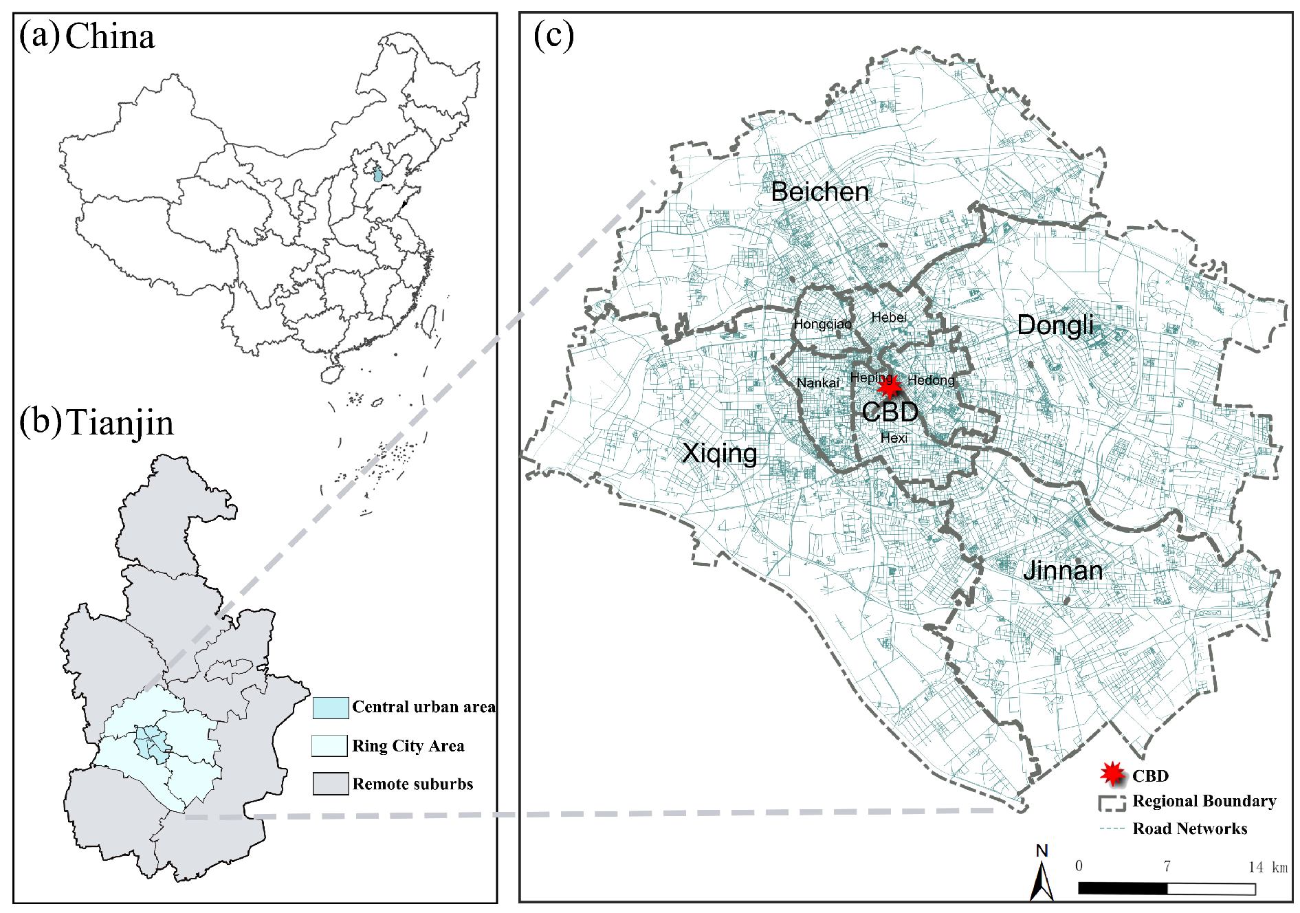
Figure 1. Overview of study area for the present study. (a) Tianjin is located in the north of China. (b) Tianjin overview. (c) Names of districts in the study area, CBD locations.
Ijgi 14 00391 g001
Figure 2. Research framework. (a) Data collection, (b) feature extraction, and (c) modeling and analysis. Arrows represent data flow between steps, and colors denote different components and relationships in the process.
Ijgi 14 00391 g002
Figure 3. Spatial distribution of (a) housing transaction price, (b) neighborhood attributes including amenities and service POIs, transportation stations, hospitals, and schools, (c) average housing price (RMB/m2) by municipal neighborhood boundary, and (d) LISA cluster analysis (hotspot) of price.Moran Scatter Plot: *** indicates statistical significance at the 0.001 level. The red line in the scatter plot represents the linear regression line for the spatial autocorrelation values.
Ijgi 14 00391 g003
Figure 4. Example of the BSVIs collection process. (a) Street view images were collocated based on OSM, and we established street view collection points at 50 m intervals.The green dots represent the locations of these collection points. (b) Boxed area in (a). (c) Panoramic street view of the points circled in (b).
Ijgi 14 00391 g004
Figure 5. Collecting perceptions. (a) Online survey system. (b) 300 Samples. (c) High/low score examples. (d) Score distribution histogram, with blue bars representing the frequency of each score level. The green and red lines indicate the mean and median scores.
Ijgi 14 00391 g005
Figure 6. Gini Importance and correlation analysis. (a) Important features in predicting five subjective perception scores. (b) Pearson correlation analysis of subjective perception scores. (c) Pearson correlation coefficient of the 7 objective indicators.
Ijgi 14 00391 g006
Figure 7. (a) Original SVI sample, (b) semantic segmentation results, (c) predicted subjective perception scores, and (d) aggregated objective perspective metrics. The radar chart displays scores and perspective metrics on a scale from 0 to 1, from the inside to the outside.
Ijgi 14 00391 g007
Figure 8. Spatial distribution of 7 street view spatial indicators.Spatial distribution of 7 street view spatial indicators. The colors range from More bad (lightest) to Very high(darkest), representing varying levels of each indicator.
Ijgi 14 00391 g008
Figure 9. Spatial distribution; 5 Perception scores. The colors range from More bad (lightest) to Very high (darkest), representing varying levels of each indicator.
Ijgi 14 00391 g009
Figure 10. Spatial Distribution of local SHAP Values for housing price determinants based on G-XGBoost. (a) Subjective perception. (b) Objective street scene indicators. (c) Location and Neighborhood attributes.
Ijgi 14 00391 g010
Figure 11. SHAP-based comparison of feature importance across different urban zones.
Ijgi 14 00391 g011
Figure 12. SHAP dependence plots of housing price drivers of subjective perception, objective street view, and neighborhood attributes to housing prices.
Ijgi 14 00391 g012
Table 1. Descriptive statistics of all variables.
VariableDescriptionMeanStdData Source
Dependent variable
PricesRMB (Chinese currency)/m2, original price26.58620.435Anjuke.com
Structural attributes
Property_TProperty type 1: Apartment house 0 for non-apartment house0.050.22Web scraping from
Anjuke.com
House_AgeAge of the building22.611.2
Year_BuiltYear of completion of the house200111.2
Floor_AreaFloor area ratio of the house1.740.73
Greening_RGreen floor area ratio of the house1.740.73
Building_TType of construction of the house, 1: multi-story 0 for non-multi-story0.340.48
Property_FProperty charges (RMB/m2/month)1.141.18
Locational attributes
Distance_tDistance to CBD (m)8694.16614.5Calculated in
QGIS
Neighborhood attributes
HubDistDistance to the nearest bus and metro station (m)196.9136.8Calculated in
QGIS
recreation_nNumber of recreational and commercial amenities within 1000 m25.419.45
school_nNumber of schools in 1000 m2424.5POI Data
hospital_nNumber of hospitals in 1000 m20.414.4
Subjective perceptions
EnclosureEnclosure perception0.670.06Predicted by ML
models with view
indices extracted
fromSVIs
HumanScaleHumanScale perception0.660.10
ComplexityComplexity perception0.700.05
ImageabilityImageability perception0.650.05
SafetySafety perception0.620.06
Objective view index
CoreStruct_ABuilding + Skyscraper view index0.460.15Scores derived
from combining
selected physical
feature view
indices
StreetSpace_B1Road + Sidewalk + Bridge view index0.280.08
TrafficInfra_B2Car + Bicycle + Minibike + Person view index0.080.03
Vegetation_C1Tree + Plant + Grass view index0.050.03
OpenNatural_C2Sky + Earth view index0.230.09
StreetFurn_DFence + Streetlight + Signboard + Awning + Ashcan view index0.020.01
ArchDetail_EWall view index0.0070.008
Table 2. Data summary of (a) view indices and (b) Gini Importance.
(a) Descriptive Summary(b) Gini Importance
SortView
Index
MeanStd.EnclosureHuman
Scale
ComplexityImageabilitySafety
1Building15.7%13.6%0.280.270.220.240.26
2Sky31.1%10.9%0.230.240.10.120.21
3Earth1.9%5.7%0.080.070.10.090.02
4Car7.2%4.7%0.070.090.10.110.08
5Sidewalk2.4%5.0%0.050.060.050.040.05
6Person0.7%0.3%0.020.060.30.40.01
7Minibike0.0%0.2%0.020.030.020.010.00
8Fence3.0%4.2%0.030.040.020.020.03
9Road28.3%9.2%0.020.020.040.070.10
10Skyscraper28.3%9.2%0.050.030.020.020.03
11Tree5.8%6.2%0.020.040.070.020.09
12Ashcan0.0%0.1%0.020.010.010.000.01
13Bicycle0.0%0.2%0.010.010.020.030.01
14Streetlight0.0%0.01%0.020.010.020.000.01
15Signoboard0.2%0.6%0.010.010.000.010.01
16Grass0.4%1.5%0.040.010.020.010.02
17Wall0.8%3.2%0.010.000.010.010.02
18Bridge0.7%3%0.000.000.000.010.01
19Plant0.7%2.0%0.000.000.000.000.01
20Awning0.0%0.1%0.000.010.000.010.01
21Van0.0%0.3%0.000.010.000.010.00
22Railing0.0%0.4%0.000.000.000.000.00
23Mountain0.0%0.1%0.000.000.000.000.00
24Fountain0.0%0.0%0.000.000.000.000.00
25Column0.0%0.1%0.000.000.000.000.00
26Ceiling0.1%2.2%0.000.000.000.000.00
27Windowpane0.0%0.0%0.000.000.000.000.00
28Chair0.0%0.0%0.000.000.000.000.00
29Sculpture0.0%0.0%0.000.000.000.000.00
30Booth0.0%0.0%0.000.000.000.000.00
Table 3. Performance and parameters of Random Forest models across perceptual dimensions.
PerceptionR2MAERMSEStd.
Dev.
Estimators
(Bootstrap)
Min Split
(Leaf)
Max Feature
(Depth)
Roy [64]
(2016)
Enclosure0.790.07890.09530.1694300 (False)2 (1)sqrt (20)Moderate
Human Scale0.630.09900.11090.1555100 (True)5 (2)sqrt (10)Bad
Complexity0.670.09550.11830.1700100 (False)10 (1)sqrt (10)Moderate
Imageability0.530.09110.11440.1765200 (False)2 (1)sqrt (30)Bad
Safety0.700.08330.12180.1754100 (True)2 (1)sqrt (10)Moderate
Note: Roy (2016) [64] classifies models with R 2 0.65 as Moderate, and R 2 0.80 as Good. Only Enclosure is close to the “Good” threshold but does not meet it.
Table 4. Regression performance and diagnostic results across different models.
Model 0Model 1Model 2
Attributes
Method
Baseline
OLS
Subjective
OLS
Objective
OLS
Adjusted R 2 (Pseudo R 2 )0.5390.5500.577
Moran’s I on Residual (p-value)0.01 ***0.01 ***0.01 ***
Robust LM (lag)601.947 ***576.633 ***648.214 ***
Robust LM (error)2174.761 ***2119.758 ***1944.270 ***
Note: p values are shown in parentheses; *** < 0.01 .
Table 5. Predictive performance of XGBoost Global and local models based on Geographical-XGBoost.
Model 0Model 1Model 2Model 3
Attributes
Method
Suburban
Ring Districts
Global Model
Central Urban
Districts
Global Model
Urban Core
(10 Districts)
Global Model
Urban Core
(10 Districts)
Local Model
Test R 2 0.5980.7100.7630.781
MAE (RMB)918.8383494.1256191.972
RMSE (RMB)2277.1176957.69010,139.574
Note: Model 3 is a local Geo-XGBoost model trained per observation; therefore, aggregate MAE and RMSE are not applicable.
Disclaimer/Publisher’s Note: The statements, opinions and data contained in all publications are solely those of the individual author(s) and contributor(s) and not of MDPI and/or the editor(s). MDPI and/or the editor(s) disclaim responsibility for any injury to people or property resulting from any ideas, methods, instructions or products referred to in the content.