Article

Automated Detection of Beaver-Influenced Floodplain Inundations in Multi-Temporal Aerial Imagery Using Deep Learning Algorithms

1
Department of Natural Resources and the Environment, University of Connecticut, Storrs, CT 06269, USA
2
Eversource Energy Center, University of Connecticut, Storrs, CT 06269, USA
3
Department of Earth Sciences, University of Connecticut, Storrs, CT 06269, USA
*
Author to whom correspondence should be addressed.
ISPRS Int. J. Geo-Inf. 2025, 14(10), 383; https://doi.org/10.3390/ijgi14100383
Submission received: 25 August 2025 / Revised: 16 September 2025 / Accepted: 25 September 2025 / Published: 30 September 2025

Abstract

Remote sensing provides a viable alternative for understanding landscape modifications attributed to beaver activity. The central objective of this study is to integrate multi-source remote sensing observations in tandem with a deep learning (DL) (convolutional neural net or transformer) model to automatically map beaver-influenced floodplain inundations (BIFI) over large geographical extents. We trained, validated, and tested eleven different model configurations in three architectures using five ResNet and five B-Finetuned encoders. The training dataset consisted of >25,000 manually annotated aerial image tiles of BIFIs in Connecticut. The YOLOv8 architecture outperformed competing configurations and achieved an F1 score of 80.59% and pixel-based map accuracy of 98.95%. SegFormer and U-Net++’s highest-performing models had F1 scores of 68.98% and 78.86%, respectively. The YOLOv8l-seg model was deployed at a statewide scale based on 1 m resolution multi-temporal aerial imagery acquired from 1990 to 2019 under leaf-on and leaf-off conditions. Our results suggest a variety of inferences when comparing leaf-on and leaf-off conditions of the same year. The model exhibits limitations in identifying BIFIs in panchromatic imagery in occluded environments. Study findings demonstrate the potential of harnessing historical and modern aerial image datasets with state-of-the-art DL models to increase our understanding of beaver activity across space and time.

1. Introduction

The North American beaver (Castor canadensis) is the largest semi-aquatic rodent in North America [1]. Beavers are ecosystem engineers which inhabit forested waterways and modify the landscape. Hydrological changes induced by beaver influence contribute to wetland formation and increasing biodiversity [2,3]. The maximum duration of beaver habitat colonization is unknown if suitable resources are present and predation pressure is low [4]. Beavers are enduring habitat loss and landscape fragmentation due to a worldwide increase in land development [5]. The decrease in core forested areas has led to loss of habitat as well as increased conflict with people. In some cases, the public and wildlife managers perceive beavers as a nuisance species. The dual perception presents a complex scenario for management strategies, as efforts to conserve a keystone species clash with the need to address human–beaver conflicts.
Beaver studies hinge on ground-based surveying methods for data collection [6]. Scalability, repeatability, and logistical challenges, coupled with intense labor and cost, stand as key limitations in conventional beaver survey methods [7]. Advanced remote sensing (RS) technologies (drone, aerial, satellite imaging), in conjunction with GIS-based mapping, offer more efficient, scalable, and accurate ways to monitor wildlife populations without compromising spatial granularity and geographical extent [8,9]. Aerial imagery is particularly valuable in ecological studies due to its higher spatial detail (~0.5 m or even finer) and spectral separability. State governments and national imaging programs in the U.S. such as the National Agriculture Imagery Program (NAIP) deploy sub-meter resolution imaging missions every 2–3 years and make data available in public domains [10]. In addition to modern multispectral images, historical grayscale aerial images dating back to the early 1930s play a critical role in an array of ecological studies, especially to understand how beavers have transformed the landscape over an ~80-year period [11]. Most regions in the U.S. lack geospatial maps delineating beaver habitats and resulting landscape alterations despite the luxury of having terabytes of aerial imagery hosted through public web portals. The utilization of large aerial image datasets in beaver studies and management activities is challenged by data volume, methodological limitations, and knowledge gaps [6]. Conventional image analysis algorithms often struggle to automatically extract information from high-resolution aerial images at landscape scale [12]. The demand is high for exploring sophisticated image analysis techniques, especially artificial intelligence (AI) algorithms in conjunction with high-performance computing resources in remote sensing of beaver habitats.
Deep learning (DL), a key branch of AI, has been showing unprecedented dominance in multiple application domains. Convolutional neural nets (CNNs) algorithms, a subset of DL techniques, have shown great promise in automated image analysis tasks [13]. Transformers which excel in natural language processing [14] are now emerging as powerful alternatives due to its innate capability in handling spatial and temporal dependencies [15]. Transformers implement a mechanism of self-attention, individually weighing the importance of each part of the input data [15]. Vision transformers (ViTs) have shown superior performances over CNNs in image classification, object detection, and segmentation tasks [16]. A considerable amount of wildlife studies have successfully integrated DL and multi-modal datasets (e.g., video data, still images, remote sensing images) models in individual animal detection [17,18], species identification [19,20], surveillance [19,21], behavioral analysis [22], habitat analysis [23,24], and animal censusing [25,26] tasks. Recent beaver studies have begun to recognize the value of integrating remote sensing with AI algorithms. Previous studies, except a few, are largely based on standard remote sensing analysis methods limited to moderate-resolution data and site-specific analysis. Zhang et al. 2023 [27] utilized moderate-resolution Sentinel-2 multispectral images, RadarSat-2 polarimetric data, and a digital elevation model (DEM) along with rule-based classification methods to map beaver ponds in Ontario, Canada. Jones et al. 2021 [8] employed manual image analysis to map beaver-induced landscape alterations in Northwestern Alaska using moderate-resolution (Sentinel-2, Landsat-8) images and high-spatial-resolution (Worldview-2) satellite images. Combining aerial LiDAR with optical images can help with identifying and reconstructing shifting patterns of surface hydrology associated with beaver ponds. Swift and Kennedy 2021 [28] used LiDAR and NAIP images, coupled with a geomorphone approach, to detect beaver impoundments and dams along the protected peatland in West Virginia. Several studies utilized unpiloted aerial systems to investigate thermal heterogeneity in beaver ponds [29]. Shallow machine learning algorithms, such as Random Forest, have been tasked to model suitable topographic and environmental conditions associated with successful beaver habitats [30]. Fairfax et al. 2023 [6] is one of the first studies which employed DL approaches to identify beaver dams from high-resolution satellite images. While their results are promising, one of the shortfalls is that the DL model was only trained to extract beaver dams. Other important structural and habitat features were overlooked because beaver disturbances extend beyond the construction of dams and associated ponds; the surrounding flooded landscape also needs to be identified to achieve a comprehensive assessment of beaver impact.
There is a pronounced deficiency in RS–AI-integrated beaver studies. We believe that this slow uptake is predominantly dictated by challenges associated with RS data volumes, veracity, semantic complexities, and computational shortfalls in running DL algorithms at scale. While a plethora of DL algorithms have been developed over the years, their performances and accuracies vary greatly. Model performance largely depends on the classification, detection, segmentation problem in hand, and the amount and quality of training data [13,31]. The direct translation of DL models from one domain to another is not always guaranteed. DL models that are pioneered in everyday tasks generally struggle to demonstrate the same level of performance when adapted to remote sensing applications due to fundamental differences in spectral, spatial, radiometric properties, seasonal variations, and imaging conditions [32]. A systematic investigation is thus required to identify the best-performing DL models. The overarching goal of our study is to close existing knowledge gaps and seamlessly integrate multi-modal remote sensing observations in tandem with a DL model to deepen our understanding of how beavers shape the New England region’s post-colonial-era forests over time. Our objectives are threefold; to (1) systematically conduct model ablation across CNNs and ViT with different encoders for beaver-inundation detection, (2) examine how image data types (multispectral and panchromatic) and seasonality affect model detection performances, and (3) apply a DL model at operational scale to generate statewide beaver activity maps from 1990 to 2019.

2. Methods

2.1. Study Area and Data

Our study area encompassed the state of Connecticut, United States (Figure 1). Land use of the state consisted of 59% forest, 19% developed, 8% turf/grass, 7% agriculture, and 7% other (barren, other grasses) in 2015 [33]. The state’s forested land had decreased by 466 km2, while developed land had increased by 403 km2, between 1985 and 2015 [33]. The expansion of developed land encroaching on forests threatens habitat availability for many wildlife species. Connecticut has a substantial beaver population as the Northeastern regions of the United States [34]. The extent of the state’s waterways and varying topography (Figure 1) provides ample habitat for the species.
In Connecticut, statewide aerial missions have been conducted since the early 1930s at varying time intervals (Table 1). Regular-interval (2 or 3 year) aerial imaging missions started in 2006 mainly through the National Agriculture Imagery Program (NAIP). Other statewide aerial data collections occurred during this period but were flown sporadically when funding was available. Image data from 1990 and 2004 are greyscale (panchromatic), all other imagery was collected with a multispectral (RGB or RGBNIR) sensor. The aerial imagery utilized in this study spanned twelve years, from 1990 to 2019, encompassing the entire state. Aerial surveys were conducted during varying times of day and across two seasons: winter (leaf-off) and summer (leaf-on), each offering unique observational conditions. Winter imagery was captured during the leaf-off period of the deciduous vegetation cycle. Leaf-on imagery was acquired during the peak growing season. The distribution of leaf-on to leaf-off imagery is uneven within the training dataset. Leaf-on images acquired by the NAIP dominate the timeseries images considered in the study relative to the leaf-off imaging missions (Table 1).

2.2. Modeling Workflow

Figure 2 indicates the key steps involved in the modeling workflow. A consistent protocol was established to ensure uniformity across image datasets from different years with varying resolutions and quality. We downloaded panchromatic and multispectral (Red (R), Green (G), Blue (B) (RGB), Near-Infrared (NIR)) aerial image scenes from the Connecticut Environmental Condition Online (CTECO) data portal. We resampled all statewide mosaics into 1 m resolution to maintain spatial resolution consistency across all years. The resampling process expedited run times of both DL model training and inference tasks. Each statewide mosaic was partitioned to smaller image tiles depending on DL architecture requirements. The semantic architectures utilized specify a (512 pxl (512 m) × 512 pxl (512 m)) tile size. YOLOv8, the instance segmentation architecture, specifies (640 pxl (640 m) × 640 pxl (640 m)) tile size. The tiling process resulted in a total of 1.09 TBs of imagery for all years. The tiles were augmented, then divided to create the three datasets, train (70%), validation (20%), and test (10%). Multiple augmentation strategies were implemented to inflate the dataset. Five copies were augmented from each original tile in the training dataset. Three architectures were tested with complementary encoder variations. Testing was performed on the highest-performing architecture to diagnose issues and conclude the effects of different training imagery.

2.3. Defining Beaver-Influenced Floodplain Inundation

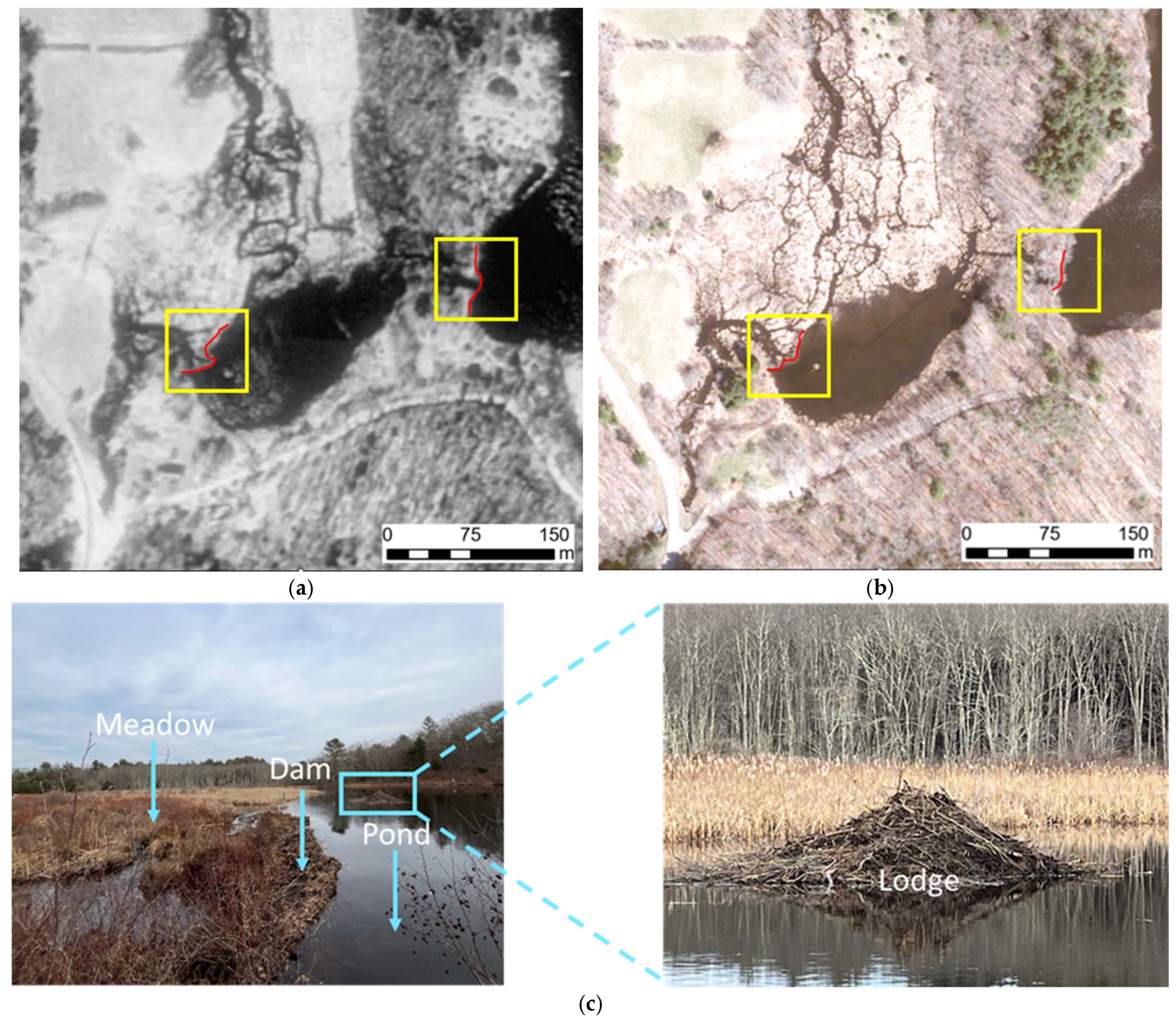
Beaver habitats were manually identified utilizing publicly accessible aerial imagery with spatial resolutions varying from ~0.8 m to 1 m (Table 1). Sub-meter resolution images capture sufficient details to detect and delineate beaver dams and the extent of environmental modifications. Beaver dams generate a distinct geomorphological signature on the landscape that facilitates detection. A river or stream carves a linear erosion pattern through the landscape in an undisturbed state [35]. The presence of a beaver dam disrupts the linear pattern, creating an asymmetrical accumulation of water. The accumulation of water results in the formation of a pond on one side of the dam, while the river continues both upstream and downstream of the obstruction [35]. Figure 3a,b depict a typical beaver habitat. The dam is evidenced by the pond formed due to the beavers’ intervention in the natural flow of the river. Figure 3a illustrates a beaver habitat identified from a leaf-off aerial image acquired in 2016. Beaver-engineered structures are visible, as seen within the outlined polygon at the coarsest resolution.
We utilized the pond and dam as two main visual cues to verify beaver habitats. Beaver ponds are defined as standing water bodies formed by beaver constructions and can vary in size depending on the extent of water accumulation post-obstruction [36]. Another indicator of beaver activity is the presence of beaver lodges (Figure 3) within ponds [37]. Employment of GIS-based identification methods allowed for the compilation of the training dataset, while negating the necessity for physical beaver habitat verification.
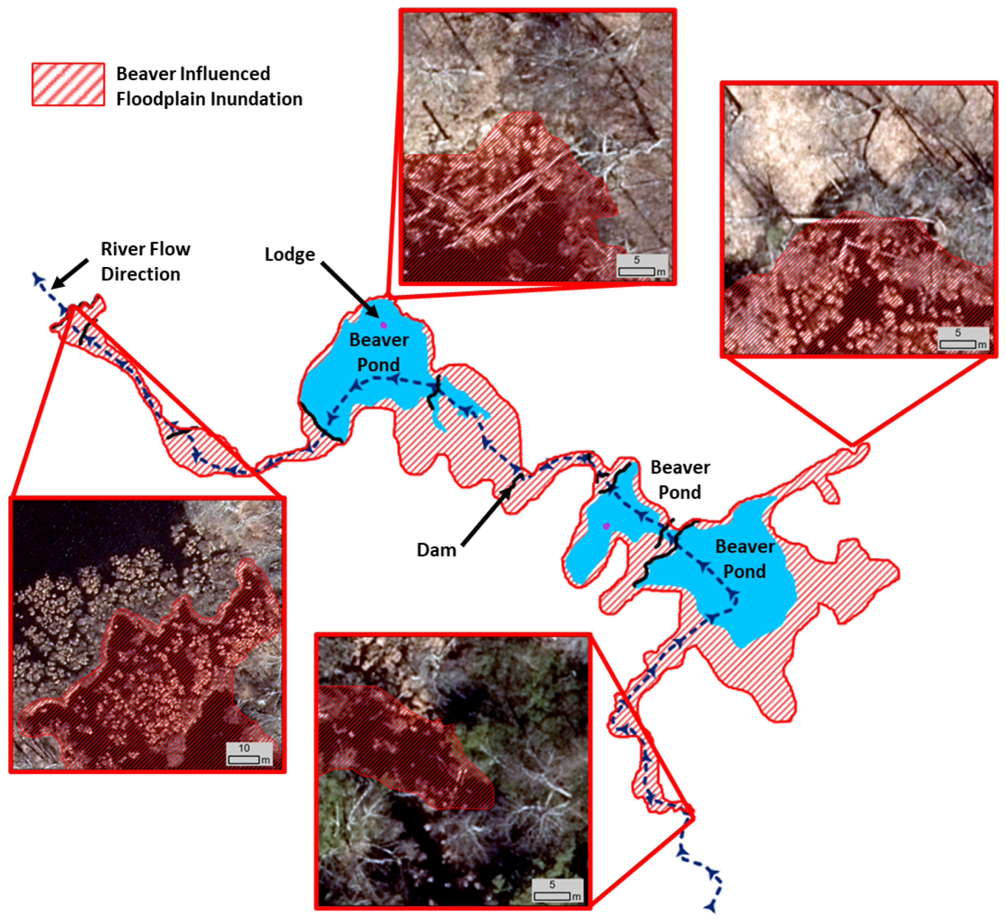
Identifying beaver habitats is primarily aimed at the field of wildlife biology and management. We wanted to assess the entire modification caused by the presence of a beaver colony. While some studies adapted terms such as beaver complex [6] and beaver territory [38,39] to describe a beaver habitat, there is a lack of consensus on an explicit definition and a distinctive anatomical description for a beaver habitat on the landscape. Dittbrenner et al. 2018 [38] defines beaver territory based on foraging ranges of the colony, typically 100 m to the lodge. Wang et al. 2019 [39] defines beaver territory from the farthest beaver-made structures. We define beaver-influenced floodplain inundation (BIFI) as land with standing water impounded though beaver obstruction(s) as detected at the time of RGB or panchromatic aerial imagery capture. Upstream extent is defined by the first impounded or diverted water pixel (1 m) that is not part of the undisturbed channel (before or after any tributaries), as inferred from visible channel structure in the captured imagery. Downstream extent is defined by the last visible beaver dam within the model’s inference window (512 m or 640 m) of contiguous pixel (1 m) standing impounded water pixels in the same channel, as observed in the captured imagery. Multiple dams and ponds may be included within BIFI if present within the same channel downstream or upstream of the inference window. BIFI is a remote sensing definition bound at the time of image capture and does not account for seasonal or external hydrological changes. There is a pronounced trade-off between annotation quality and quantity. Thus, adaptation of formal class definition for BIFIs helps guide the manual digitization task to produce a consistent and accurate training dataset. BIFI encapsulates one or more beaver habitats as the flooding from a beaver habitat creates part of the total BIFI (Figure 4). The border of the BIFI highlights the difference between the included inundated land and the visual appearance of dry land. A BIFI can incorporate multiple beaver ponds with multiple dams or a single habitat with one dam.

2.4. Compiling Training Dataset

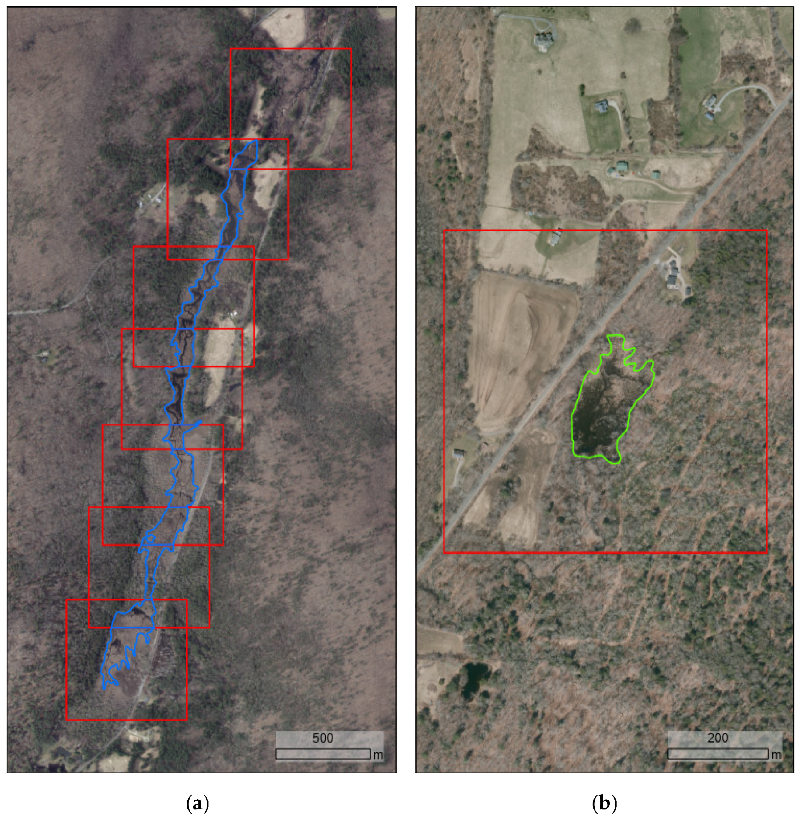
The final training dataset was compiled from 600 BIFIs from twelve years of RGB/Panchromatic aerial imagery. Each annotation required multiple additional tiles to ensure full cover where BIFIs extend beyond a 640 pxl × 640 pxl tile boundary. The border of a BIFI was delineated by the absence of any beaver structures for a distance exceeding 640 m. The 640 m criterion was based on the observation that multiple beaver colonies may coexist within a single riverine network. The operational definition of a BIFI’s boundary can vary across different studies. In this study we chose 640 m as the maximum distance between a single BIFI to coincide with the YOLOv8-recommended tile size. A BIFI with a distance larger than the tile size between beaver-influenced floodplain inundation could not be included in a single annotation. The scenario shown in Figure 5a depicts a BIFI that requires multiple tiles to properly encapsulate, while the BIFI shown in Figure 5b requires only one tile. Two datasets were made to correspond to the two required training dataset image size requirements. The semantic architectures (SegFormer and U-Net++) were trained on a separate ratio to the instance structure (YOLOv8). SegFormer and U-Net++ input 512 pxl × 512 pxl image tiles. The YOLOv8 architecture requires 640 pxl × 640 pxl image tiles. Two datasets with the same training data using different tile sizes were generated.
Deep learning models require a large variety (shape, size, direction) of training samples to accurately identify and classify targeted objects [40]. It is therefore advisable to have a training dataset that captures a wide array of variations in the target object, as well as diverse examples of potential backgrounds. Similar models identifying natural objects have upwards of 10,000 training samples to align with industry standards and enhance model accuracy [6]. Image augmentation techniques were employed to increase the heterogeneity of the targets of interest and to inflate the volume of the dataset. Beaver-influenced floodplain inundations can form in various orientations relative to the landscape. Training the model to recognize BIFIs from multiple angles theoretically improves its ability to detect BIFIs regardless of their orientation [41]. The instance training dataset includes 8463 annotations. After augmentation, the 640 pxl × 640 pxl dataset (38,083) was split into 70% training (35,544), 20% validation (1701), and 10% testing (838). The 512 pxl × 512 pxl dataset included 11,087 annotations. The training dataset (49,887) was split into 70% training (46,560), 20% validation (2229), and 10% testing (1098) after augmentation. Background or blank images that were added to the dataset after initial testing showed confusion with leaf-on imagery. Blank images do not contain object pixels, increasing regularization to the background class when included. Initial tests in leaf-on imagery showed high percentages of false positives. False positive images were included as blanks in the dataset from leaf-on imagery. All the model training, testing, and operational deployments were implemented on a workstation equipped with a hardware configuration of Intel(R) Core(TM) i9-10900X CPU @ 3.60 GHz with twin NVIDIA RTX A4500 GPUs.

2.5. Deep Learning Model Training

Two categories of deep learning segmentation models were tested in this study. SegFormer is a semantic segmentation transformer architecture. Transformers can capture long-range dependencies while being computationally efficient [42]. The Mixed Vision Transformer encoder is hierarchical, extracting multi-scale features. The SegFormer decoder fuses features for pixel-level predictions [42]. The entire model was trained with no frozen sections. Multiple model variants were tested: B0-Finetuned (~3.8 M parameters), B1-Finetuned (13.8 M parameters), B2-Finetuned (27.5 M parameters), B3-Finetuned (47.3 M parameters), and B4-Finetuned (64.1 M parameters). B0-Finetuned is typically used in small, lightweight tasks while B4-Finetuned is recommended for relatively complex tasks [42].
U-Net++ is a semantic CNN architecture that was trained on the training dataset. It is an improved version of the U-Net architecture featuring nested skip pathways to refine feature maps [43,44]. Skip connections allow for higher-accuracy semantic feature fusion and gradient flow. U-Net++ is flexible and is improved for complex segmentation. The entire model was trained with no frozen sections. Four encoders were tested; ResNet-18 (~11.7 M parameters), ResNet-32 (~21.8 M parameters), ResNet-50 (~25.6 M parameters), ResNet-101 (~44.5 M parameters) [43,44]. ImageNet was used as the decoder for all four model trains.
The You Only Look Once, version 8 (YOLOv8) is an instance segmentation CNN architecture. YOLOv8 has a reputation for accurate segmentation capabilities with a relatively simplistic training dataset (<10,000 annotations) [45,46]. The DL architecture divides an image into a grid containing pixel values. If the center of the object to be detected falls into a grid cell, that cell detects that object [40,46]. Confidence is scored for each inference depending on an earlier trained model depicting desired pixel values/surrounding values [40]. Multiple detections are made per grid cell, yet the algorithm filters by confidence scores to only include specified detections. Five model variants, YOLOv8n-seg (~3.2 M parameters), YOLOv8s-seg (~11.2 M parameters), YOLOv8m-seg (~25.9 M parameters), YOLOv8l-seg (~43.7 M parameters), and YOLOv8x-seg (~68.2 M parameters), were tested with YOLOv8.
Ten separate models were created from the three architecture types. Five SegFormer, four U-Net++, and five YOLOv8 models were constructed with the previously specified range of encoders (Table 2).
Loss metrics were observed during the training process to understand potential issues. Loss metrics identify different flaws that exist within the datasets. Through the calculation of loss errors in training, data can be assessed for later improvement [40]. Binary Cross Entropy Loss (BCEL) was used for both U-Net++ and SegFormer’s model trains. YOLOv8 uses a custom-built segmentation loss function which implements the logic of BCEL. The best epoch selected for each model was considered when validation loss was at its lowest.
B C E L y p r e d i c t i o n , y t r u e = [ y log y ^ + 1 y log 1 y ^ ]
We utilized standard accuracy metrics to assess the model performances on the hold-out test data including precision, recall, and F1 scores. Precision measures the model’s exactness, determining the proportion of true positive (TP) inferences out of all positive inferences (TP + FP) made by the model [45]. Recall assesses the model’s ability to identify all relevant instances, calculated as the number of true positive inferences divided by the sum of true positives and false negatives (FN) which are missed true BIFIs [45]. The F1 score is a harmonic mean of precision and recall, providing a single metric that balances both values [45]. F1 scores are especially useful when the distribution of the class categories is uneven. A model exhibiting high values in precision, recall, and F1 score is considered successful. All three metrics collectively offer a nuanced overview of the model’s ability to inference BIFIs accurately and reliably [45].
P r e c i s i o n = T P T P + F P R e c a l l = T P T P + F N
F 1 = r e c a l l     p r e c i s i o n r e c a l l   +   p r e c i s i o n     2
Certain model specifications were held constant between the different architecture trains. Patience was set to 10 epochs to conclude training when validation loss increases. Learning rate started at 1 × 10⁻⁴, then a cosine annealing derived from the learning rate scheduler was implemented.

2.6. Training Data Ablation

Imagery utilized in this study varies in the number of bands and acquisition dates. Three individual training data models (each containing a single imagery type) and one blended model (containing all imagery types) were generated to assess the impact mixing varying image types had on identifying BIFI. The three “unblended models” consisted of panchromatic leaf-off, RGB leaf-off, and RGB leaf-on imagery. Each model was tested on corresponding unseen imagery of the same dataset. The blended dataset consisting of all three imagery types (RGB leaf-off, RGB leaf-on, Panchromatic leaf-off) was tested on blended test data and the other three models’ test data for comparison.

2.7. Straight-Edge Post-Processing Methodology

A post-processing methodology was created and implemented on the highest-performing models’ inferences to correct errors caused by tile size, random image tiling, and images lacking context to delineate the BIFI. Straight edges of inference polygons greater than or equal to 50 pxl were identified in inferences. The direction of the straight edge was calculated, and another image tile was mosaicked to fill in the gap in context. The additional tile consisted of half of the previous tile and half of the data missed by the inference. The newly generated image had higher context in regions clipped by the tiling process. The mosaicked image was inferenced on by the same model creating a completed BIFI. Post-processing continued through successive iterations until all partial outputs were finalized. All inferencing was performed at 75% confidence.

2.8. Visual Quality and Map Accuracy Assessment

A pixel-based map accuracy assessment was performed to test overall performance on a region unseen by the model. Two regions were chosen for pixel-based map accuracy assessments. The first was the Ipswich watershed in Massachusetts (MA) comprising 401.4 km2. Ipswich served as an unseen region similar to the training dataset region (Connecticut). The imagery was collected in 2021 in leaf-on conditions in an aerial statewide flight. Ipswich, MA, imagery was resampled to 1 m to match the training data. We randomly selected 2000 pixels to be manually validated on inferences constructed from the model at 75% confidence. A visual inspection of inferences was conducted to determine each architecture’s ability to interpret BIFI. True positives, false positives, false negatives, and true negatives were assessed to analyze possible errors within each model. Interpretation based on the assessments led to further changes to the training dataset. The Umpqua watershed in Oregon served as an unseen region unique to the training dataset. The total area is 13,355 km2. The aerial imagery was collected in 2018 in leaf-on conditions. The density of BIFIs in the Oregon region is lower than that in New England, requiring a different analysis. Each inference was identified as a true or false positive. Analyzing a random set of 2000 pixels provided little to no BIFIs (<5). The alternative method assessed the model’s ability to identify the trained object in a unique region to the training data. All inferences were analyzed at 75% confidence to conclude if a true BIFI was detected. True and false positive percentages were recorded.

3. Results

3.1. Training Dataset Analysis

The hand-annotated beaver-influenced floodplain inundations (BIFI)s were graphed to summarize the temporal partitioning (Figure 6). Sixteen percent of hand annotations were based on panchromatic imagery, 58.2% were leaf-on imagery, and 25.8% were leaf-off imagery. The percentage of panchromatic images was relatively low, reflecting that panchromatic imagery was collected in two non-consecutive years and few BIFIs were present. Two panchromatic image scenes were utilized for a total of twelve years while the remainder were RGB or RGBNIR. Summer imagery, RGB leaf-on, constitutes the majority due to the amount of aerial flights occurring during the agricultural peak season captured by NAIP. Spring imagery was also collected in RGBNIR, but the difference in the forest canopy from both seasons changes the quality of imagery requiring separate analyses.

3.2. Model Performance

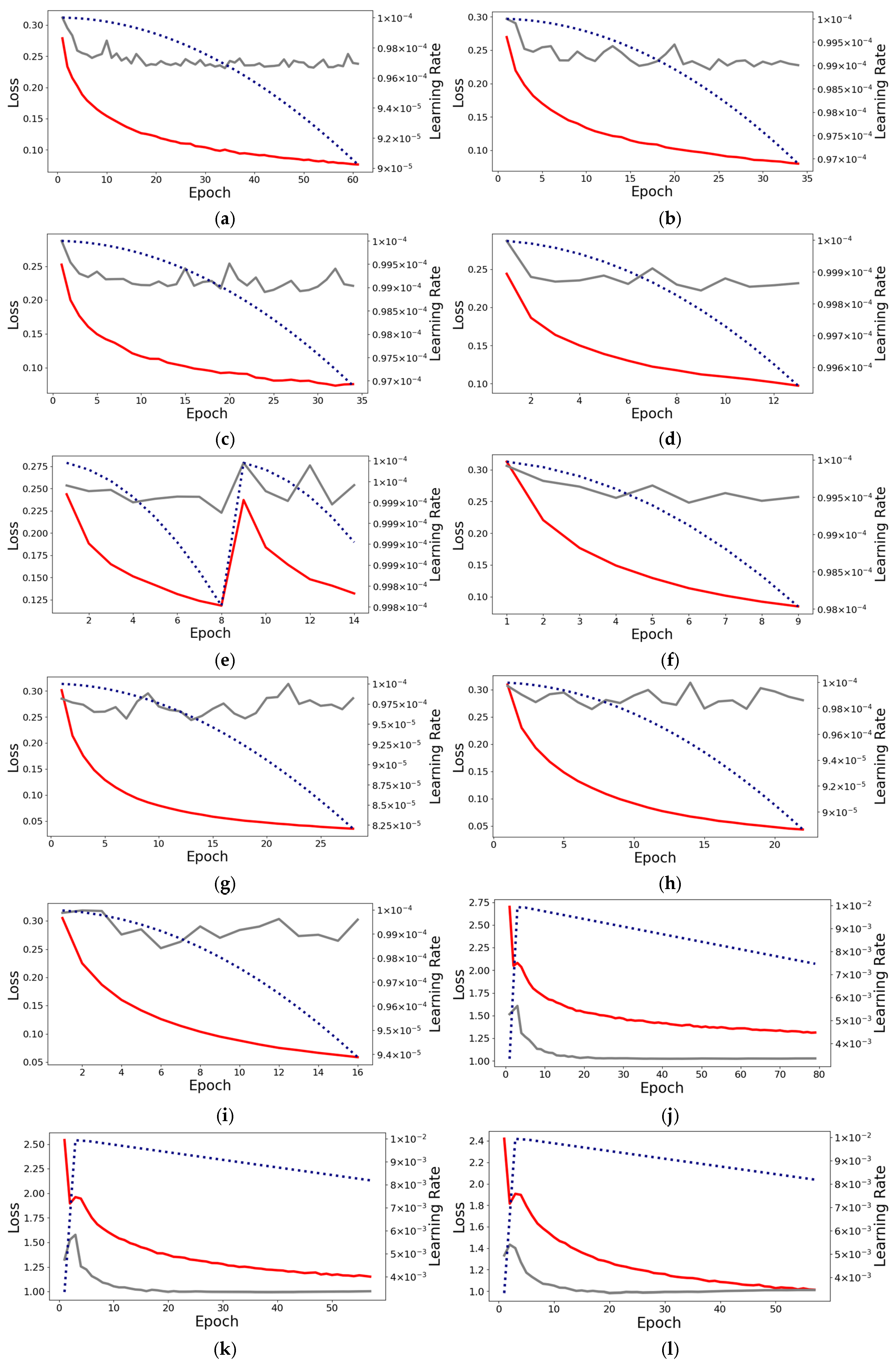
Loss metrics indicated details on model performance through the training process. The SegFormer model with encoder B2-Finetuned trained with the lowest validation loss of 0.21 at epoch 24 (Figure 7c). The highest-performing overall SegFormer model train was encoder B3-Finetuned at epoch 9 with a train loss of 0.11 and validation loss of 0.22. U-Net++ with ResNet-34 had the lowest train (0.07) and validation loss (0.24). U-NET++ with the ResNet-34 encoder had the highest overall F1 score at epoch 13 (Figure 7g). YOLOv8l-seg’s highest-performing model had a train loss measurement of 1.17 and validation loss of 0.97. The highest-performing epoch for YOLOv8l-seg was 25. The highest-performing models of each architecture were compared against one another, revealing the different loss values. The YOLOv8 configurations measured relatively high loss compared to the other architectures.
F1 model comparison on unseen test data revealed the performance of each model using the best epoch (Table 3). SegFormer B0-Finetuned displayed the weakest ability to recognize BIFI, with an average F1 of 0.5202. The highest-performing SegFormer encoder was B3-Finetuned, with an F1 of 0.6834. The lowest-performing U-Net++ encoder was ResNet-18, with an F1 of 0.7605. The highest-performing U-NET++ utilized the ResNet-34 encoder, with an F1 of 0.7802. YOLOv8l-seg was the highest-performing model, with a test F1 of 0.8059. All model results were compared to identify the highest-performing model across the test image dataset.

3.3. Training Data Ablation Analysis

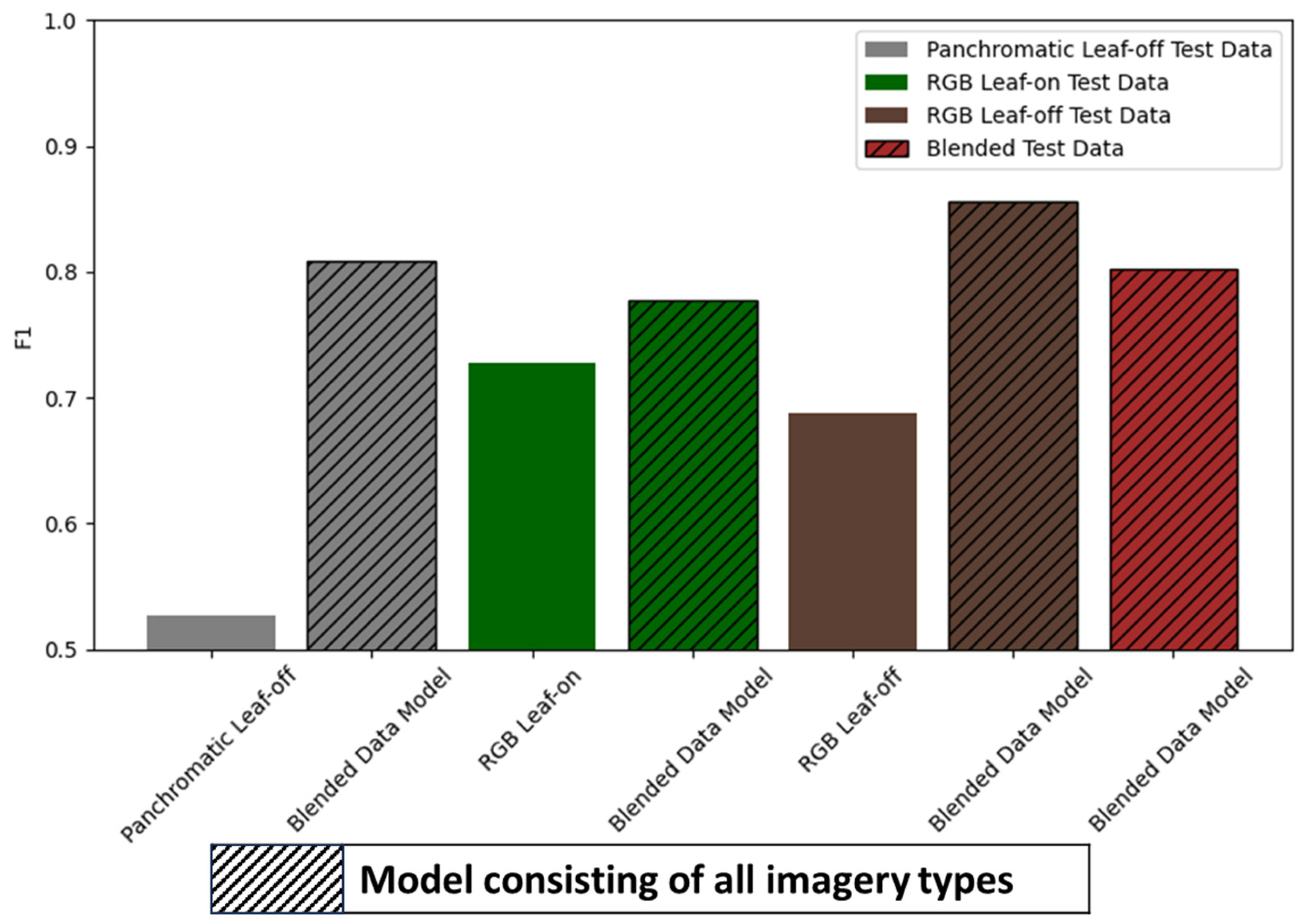
Figure 8 depicts the highest-performing model, YOLOv8l-seg, which was trained with a dataset split by data type (panchromatic leaf-off, RGB leaf-on, and RGB leaf-off). The panchromatic leaf-off dataset had the lowest-performing F1 (0.5275). The blended model performed 0.2816 F1 higher on panchromatic-only test data. RGB leaf-on F1 performed 0.0500 F1 lower on RGB leaf-on test data compared to the blended dataset. RGB leaf-off F1 performed 0.7271 on the RGB leaf-off-only test dataset, while the blended model performed 0.1673 higher F1. The blended dataset performed higher F1 when inferencing RGB leaf-off data when compared to blended test data.

3.4. Straight-Edge Post-Processing Method

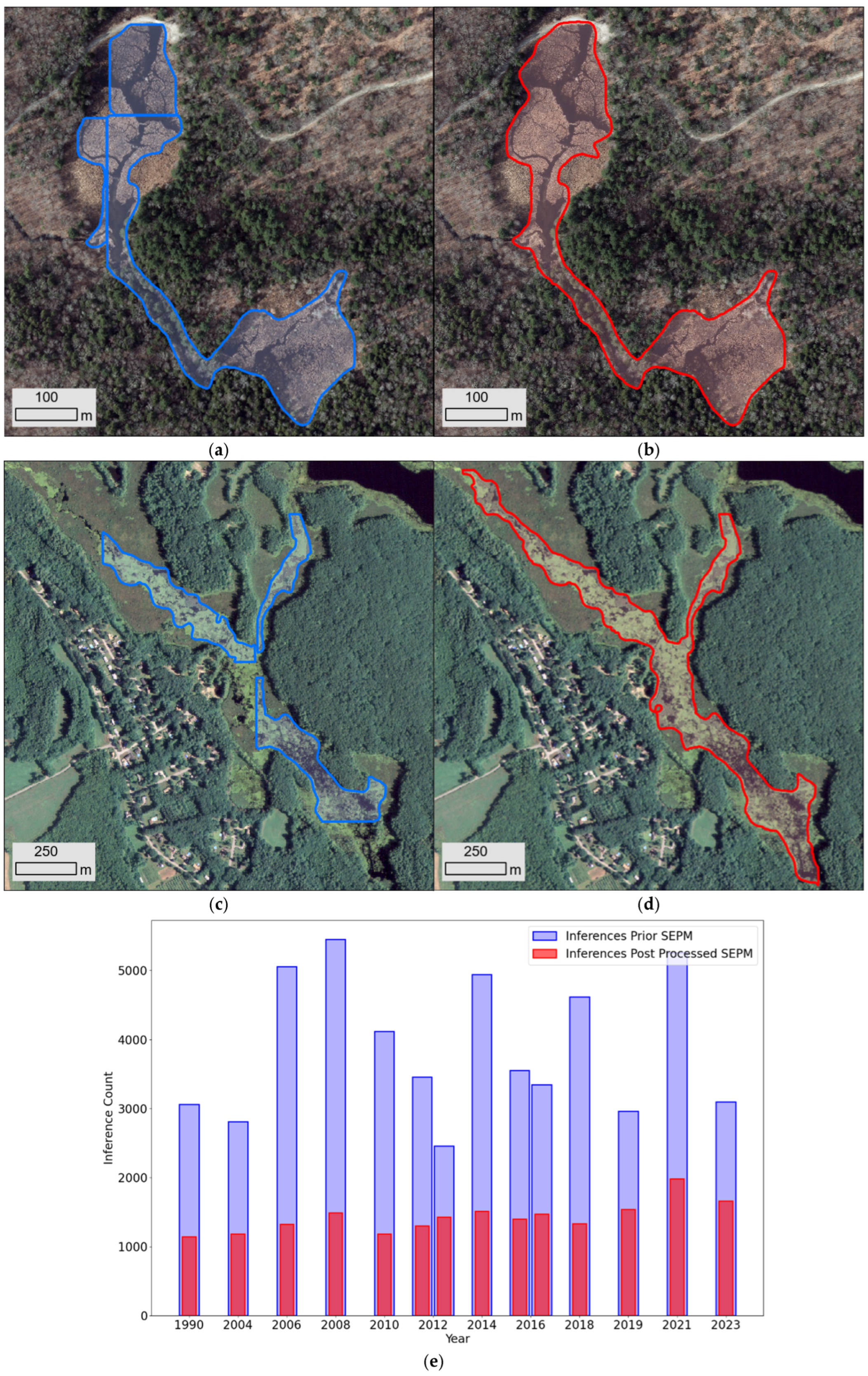
The results of the straight-edge post-processing method (SEPM) on total BIFI were recorded and compared against non-post-processed results to indicate utility. The average difference was 2448 with a minimum of 1025 (2012 leaf-on RGB) and a maximum of 3969 (2008 leaf-on RGB). Figure 9a shows leaf-off RGB inferences which missed portions of BIFI found in the post-processed BIFI (Figure 9b). Figure 9c exemplifies obstructions which prevented entire BIFI inferencing before the implementation of SEPM (Figure 9d). The post-processed BIFI (Figure 9d) connects the two portions of BIFI while expanding edges missed in the original inferencing method. Prior to SEPM implementation, the inference count was higher for all inferenced years. SEPM filled in the inference gaps, providing a more accurate count for definition.

3.5. Statewide Beaver-Influenced Floodplain Inundation Detection

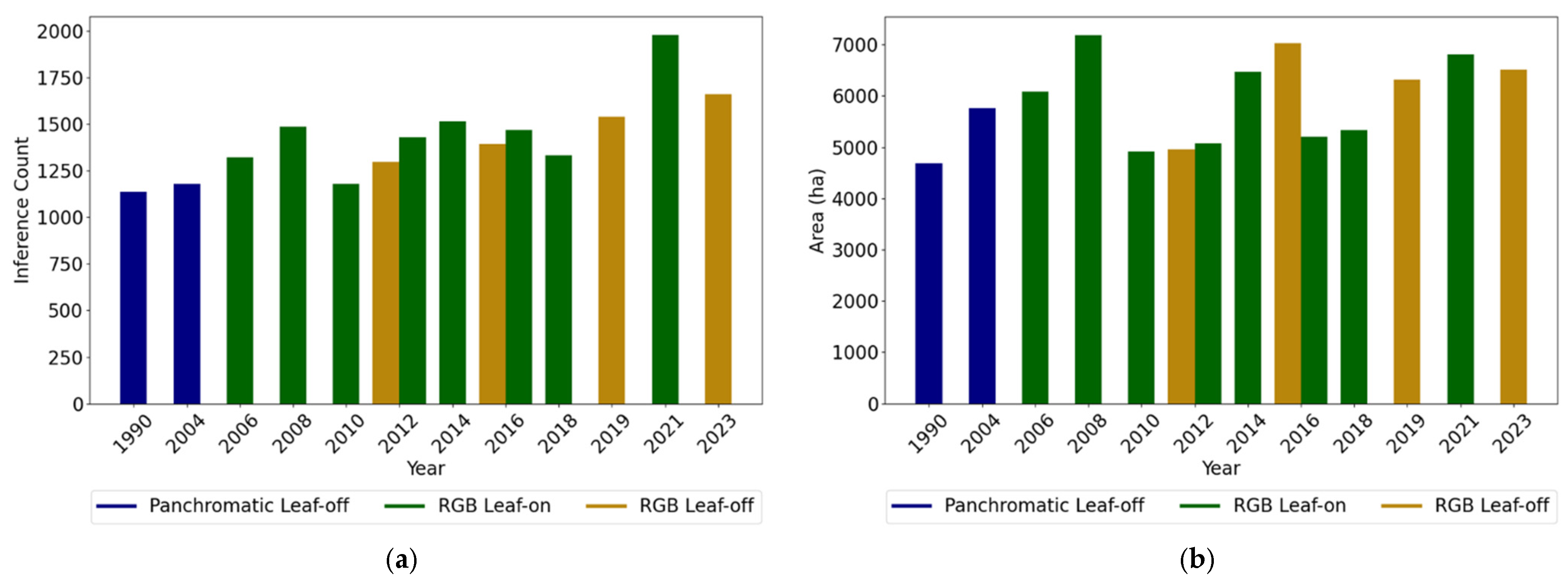
The model with the highest performance, YOLOv8l-seg, was deployed on 14 statewide captures of Connecticut aerial imagery for the localization of BIFIs. The output contained polygons delineating regions inundated by beaver activity, as specified in the investigation. The entirety of flood inundation was quantified and logged in hectares. Data from 1990 uncovers a notable trend: an increase in identified BIFIs, yet varying cumulative areas. The number of BIFIs and total modified area were graphed to further analyze patterns (Figure 10). The amount of BIFI inferences increased by 522 from 1990 to 2023. The 2021 RGB leaf-on had the higher number of inferences (1979). The lowest amount of inundated area was in 2010 with 4921 ha. The year 2008 had the largest amount of inundated area (7030 ha). A 5 km inland buffer zone was established along the Connecticut coastline to omit coastal false positives.
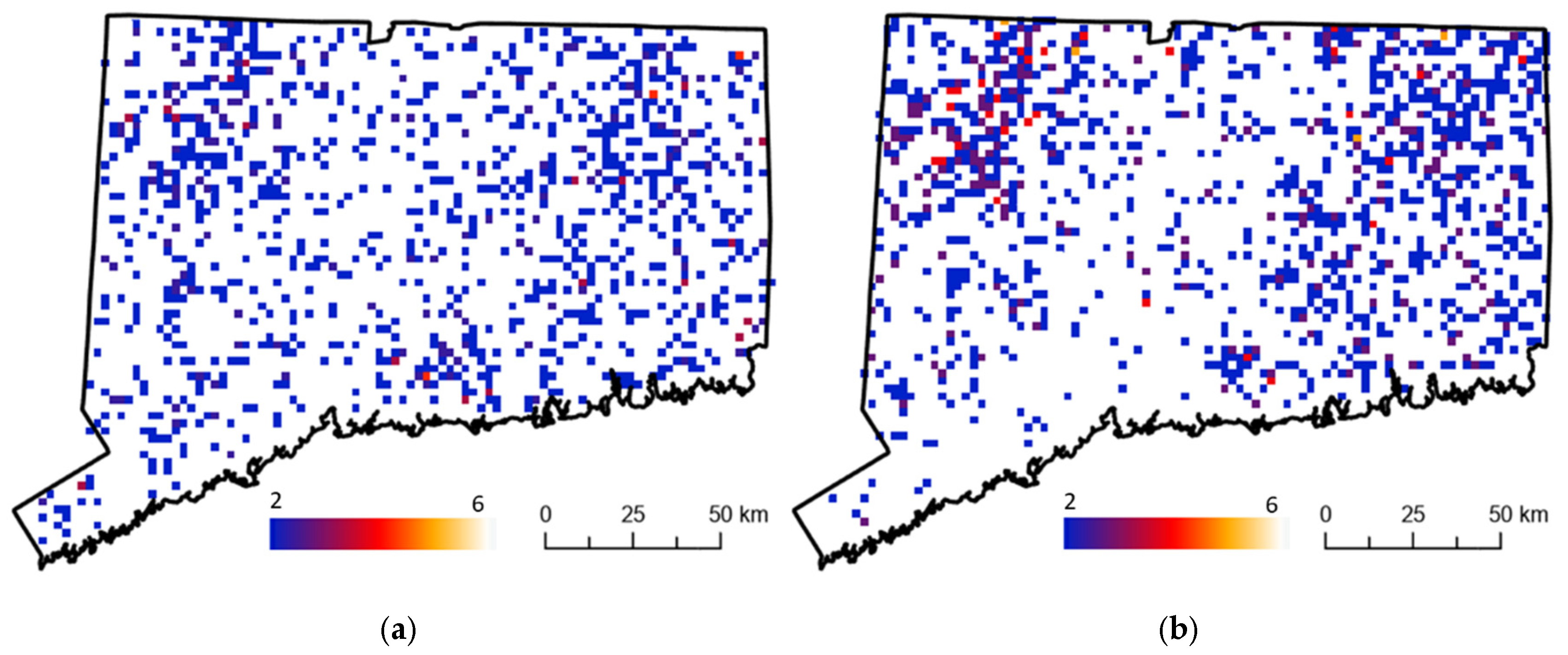
Density maps delineating the statewide-distribution of BIFI inferences were developed to further analyze the spatial distribution. Density maps employed graduated symbols across a 5 km2 grid to depict variations in BIFI density in 1990 and 2019. The 1990 map (Figure 11a) indicates a uniform distribution of inferences across the state. In 2019 (Figure 11b), there was a noticeable concentration of BIFIs within Northwestern Connecticut.

3.6. Visual Quality Assessment

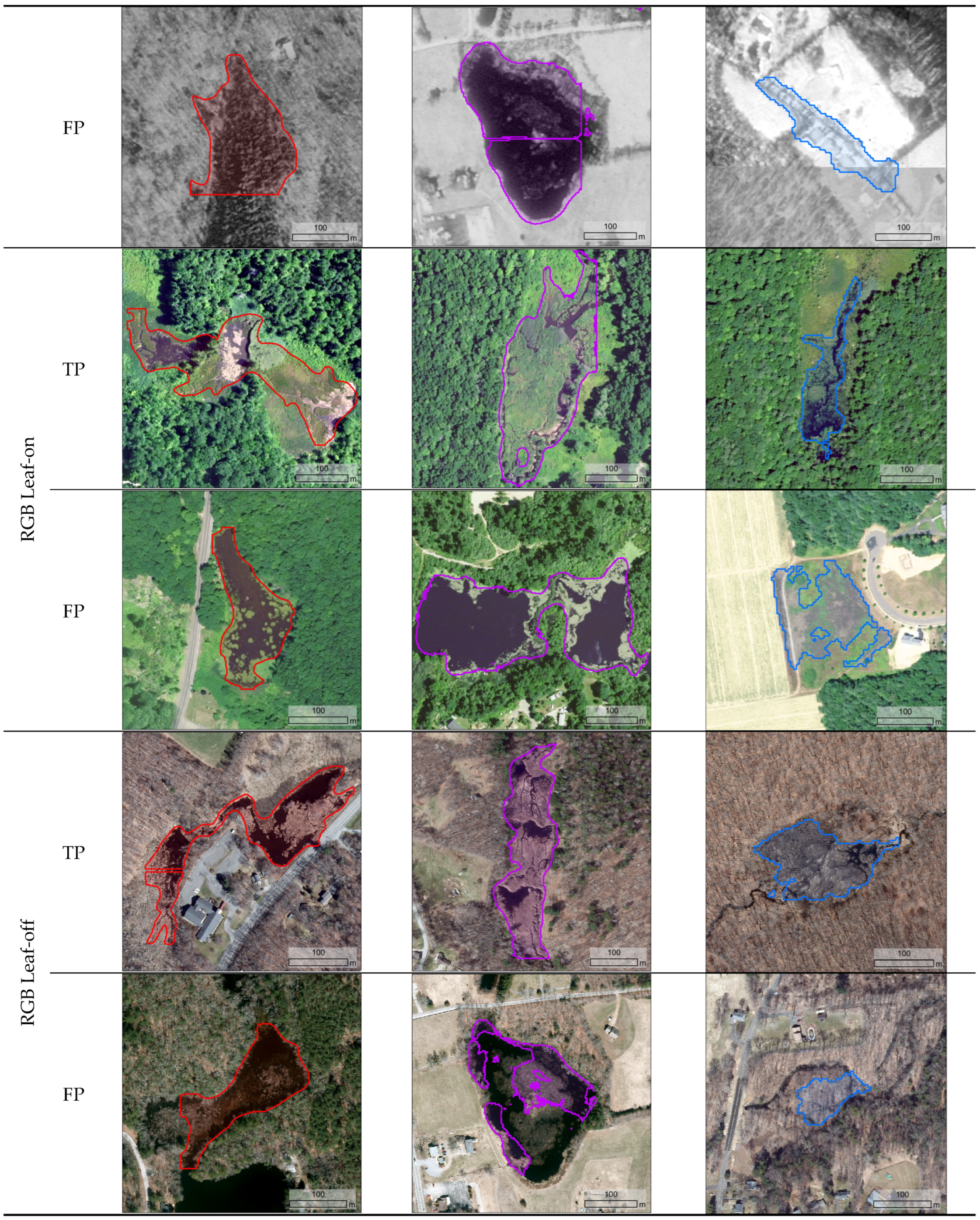
Inferences from each architecture’s highest-performing model were compared to determine the model performance on each imagery type within the training dataset (Figure 12). The YOLOv8-derived inferences created accurate boundaries within panchromatic leaf-off imagery capturing the entire BIFI. U-Net++ captured the entire BIFI but contained areas of over-segmentation where the dam meets the edge of the forest. The SegFormer model over-segmented and under-segmented BIFI throughout inferences. YOLOv8 and U-Net++ both captured segment waterbodies as false positives. The SegFormer model mistook buildings as BIFI in multiple instances. RGB leaf-on imagery showed improved boundary delineation relative to panchromatic leaf-off. The submergent vegetation caused some occlusion but, overall, the boundaries were successful in all true positives. False positives were similar for YOLOv8 and U-Net++ when compared to panchromatic imagery. Ponds with submergent vegetation confused the model, causing mistakes. All models performed the highest-accuracy boundary delineation with leaf-off imagery. Inferences were free of occlusion, capturing the full extent of the BIFI without including unaltered water ways. False positives occurred in small waterbodies with vegetation presence or in instances where river veining occurred without beaver modification.
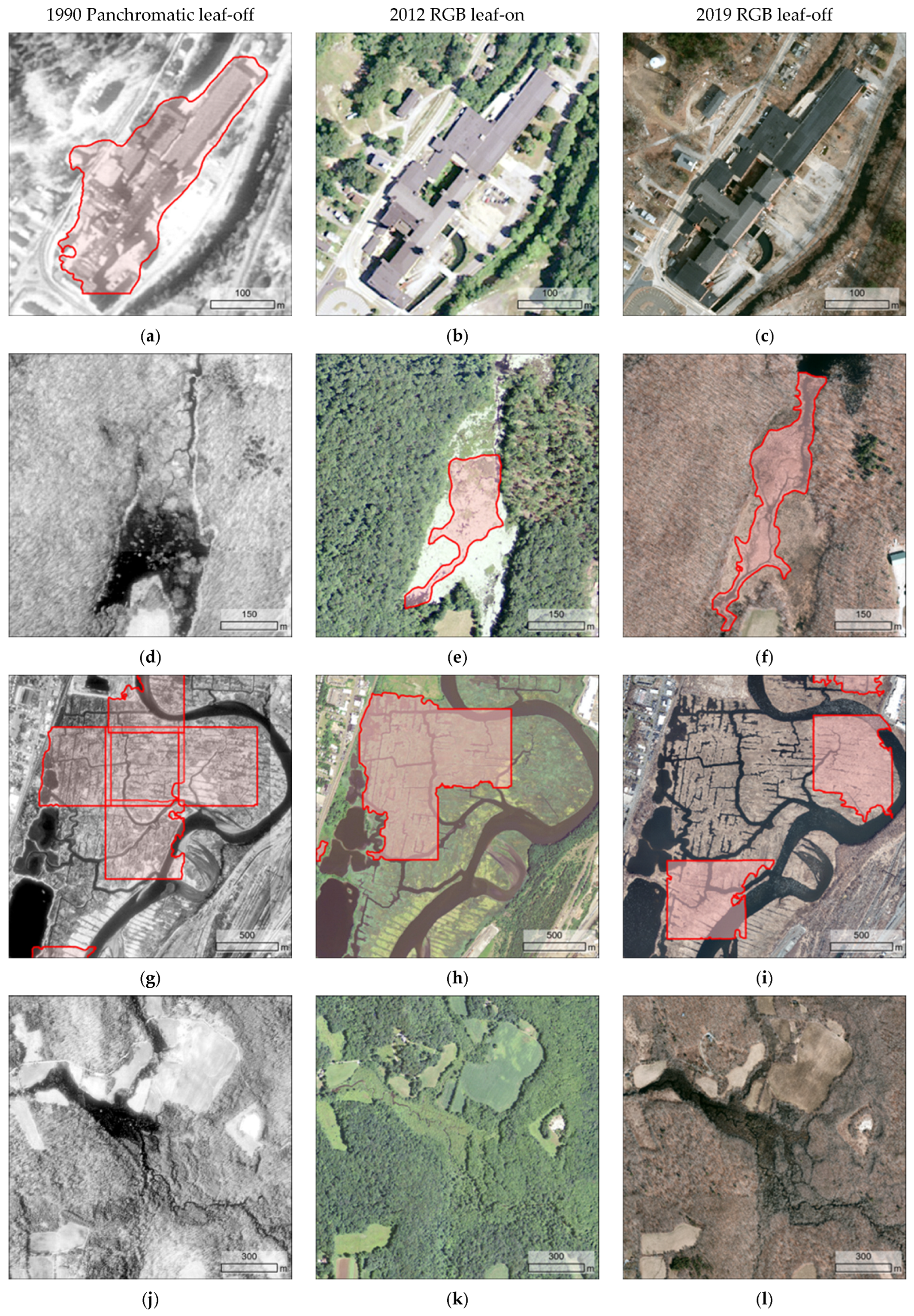
We corroborated quantitative analysis with thorough visual assessments to evaluate the quality of model detection and segmentation using the YOLOv8l-seg model. A set of example model inferences were chosen for three years, 1990, 2004, and 2019, for comparison. The BIFI denoted, as Figure 13a–c show, no signs of beaver activity in the 1990 image (Figure 13a). A beaver dam had been constructed by 2004, altering the flow of a previously uninterrupted stream (Figure 13b). The BIFI expanded in 2019 as the dams were positioned differently compared to 2004 (Figure 13c). The repositioning of dams at strategic locations had altered the morphology of the BIFI, increasing the flooded area between 2004 and 2019. The model had correctly identified this change by encapsulating the entire area of the BIFI in both Figure 13b,c. The BIFI shown in Figure 13d–f displays minimal change throughout the three periods. The number of dams in the 1990 image is slightly lower than in 2004 and 2019, yet their placement remains consistent. BIFIs can show no change over decades. The model correctly identified that no change had occurred and properly outlined the BIFI. The limitations of the model were apparent in cases where BIFI details were occluded. Although no BIFI was detected in 1990 (Figure 13g), evidence of beaver activity within the highlighted area appeared in 2004 (Figure 13h). The model missed the BIFI initially, then identified it in 2019 (Figure 13i) when the evidence became more pronounced. Beaver-influenced floodplain inundations with minimal landscape impact present a challenge for the model to confidently infer. Certain BIFIs do not grow in area over time in all scenarios. Beaver-influenced floodplain inundations that shrink in area over time were observed to test the model’s ability to accurately predict BIFI areas. A BIFI in 1990 (Figure 13k) was present with multiple dams. In 2004 (Figure 13l) a BIFI increased in area and the model accurately identified the change. In 2019 (Figure 13) the BIFI reduced in total area, reflecting the 1990 (Figure 13k) inference.
The issue of leaf-on imagery occlusion was further explored by comparing various BIFIs using both leaf-on and leaf-off imagery. A leaf-on inference collected from 2018 leaf-on imagery (Figure 14a) highlighted occlusions from deciduous trees and emergent aquatic vegetation. In 2019, leaf-off imagery (Figure 14b) of the inference on the same BIFI led to a larger depicted area. The juxtaposition of both inferences underscores the impact of occlusions in reducing the perceived area in leaf-on imagery when compared to the actuality in the leaf-off imagery (Figure 14c). The showcase of both inferences represented a challenge for the model, as it led to inaccuracies in estimating the total area of BIFI inferences during leaf-on imagery seasons. The occlusion-inaccuracy issue is further explored in another BIFI where no inference was made though evidence of beaver activity was present. The 2018 RGB leaf-on imagery identified a BIFI (Figure 14d) where no inference was made despite evidence of beaver activity. In 2019, RGB leaf-off image (Figure 14e) of the same BIFI is shown with the correct inference, validating the presence of beaver activity.
Issues with YOLOv8l-seg inferences were analyzed to detect the impact of different imagery types. Panchromatic inferences contained false positives of buildings that were not present in leaf-on or -off imagery (Figure 15a–c). Also, BIFIs were detected with higher difficulty when compared to later years (Figure 15d–f). Coastal false positives existed within all three types of imagery (Figure 15g–i). The model failed to pick up BIFIs throughout the three years of imagery that are not occluded and identifiable through human detection, showing inferencing challenges (Figure 15j,k).

3.7. Map Accuracy Assessment

The pixel-based map accuracy assessment in Massachusetts consisting of the Ipswich watershed showed 98.95% correctly inferenced pixels. The percentage object pixels (3.90%) and percent background pixels (96.1) showed a clear majority of background within the sampled region (Table 4). A higher percentage of false negatives (0.65) than false positives (0.40) were observed in the Ipswich analysis. The Umpqua River watershed, Oregon (OR) map accuracy assessment displayed a 99.9% accuracy of assessing background imagery. The assessment was flawed due to the density of sites requiring additional analysis (Table 5). An analysis of inferences of the Umpqua River watershed recorded a 13.27% true positive compared to 86.73% false positive.

4. Discussion

4.1. Training Dataset Analysis

The central goal of our study was to systematically investigate the performance of multiple deep learning architectures when applied to the beaver-influenced floodplain identification (BIFI) detection task. We explored how models react to perturbations in training data that are largely due to seasonal variations, vegetation phenology, and imaging sensors. Scalable model inference pipelines were also evaluated to assess the feasibility of producing regional BIFI maps from multi-temporal aerial imagery, including both historical and modern datasets. Our training dataset consisted of RGB leaf-off, RGB leaf-on, and panchromatic leaf-off images at a split of 58.2%, 25.8%, and 16%, respectively (Figure 6). When pooled, the imbalance in training samples, for example, under-representation of grayscale images, dictated fluctuations in DL model performances. The leaf-off image samples offered unobstructed views of BIFIs to the model trains whereas the deciduous canopy in leaf-on image samples that were annotated based on NAIP images tended to obscure important morphological characteristics of the BIFI. Panchromatic leaf-off imagery provided the advantages of limited occlusion, but at the expense of a limited number of training samples and spectral details. Emergent aquatic vegetation further complicated the manual annotation process by causing water bodies to be identified as terrestrial features, which introduced spatially inaccurate BIFI training samples to the training dataset. The occlusion issue present in the NAIP leaf-on imagery affected the boundary accuracy of most of the hand-annotated BIFI instances. Lack of visual cues due to canopy obstruction caused human analysts to generalize BIFI boundaries during the annotation process. This boundary fuzziness led to both over-estimation and under-estimation of actual spatial extent and geometry. BIFI boundary delineation inflates when at the periphery of BIFIs. Annotation uncertainty propagated throughout the model affected the final area calculations. Compared to leaf-off imagery, canopy obstructions in leaf-on images led to incomplete segmentation results across all years. Joshi and Witharana, 2025 [47] studied the effects of annotation uncertainty on model performance and the downstream results through their analysis of tree-canopy modeling. To test for variability in annotation, nine annotators were given a canopy annotation protocol to follow, then tasked to digitize thirty unique image patches. Comparison of peer annotations demonstrated high variability between the definition of the object of interest. Thus the variability in annotation due to canopy occlusion can cause large fluctuations in model performance, as demonstrated in the uncertainty analysis by Joshi and Witharana, 2025 [47]. Seasonality affected the level of inundation and/or area inferenced. BIFI area increased with inundation that occurred in the panchromatic and RGB leaf-off imagery due to winter accumulation. RGB leaf-on inference area was lower, potentially due to a recharge deficit from evaporation and evapotranspiration. Nathan and Bimber, 2023 [48] studied the effects of canopy occlusion on object-detection models. Detection of objects in areas of dense canopy produced false detections through large pixel clusters, augmenting the true target’s shape. Both the target visibility and precision of detections dropped as forest density increased. Detection in dense canopy without removing occlusion led to inaccurate detections and under-performance of the trained model. The concept of leaf-on forest-canopy occlusion is further examined in Waser et al., 2021 [49]. In this study they developed a workflow which incorporated Sentinel-1 and Sentinel-2 leaf-off and leaf-on imagery to map dominant leaf type. A U-Net model with an overall accuracy of ~0.97 demonstrated the potential to differentiate between broadleaf and coniferous tree species. Leaf-on and leaf-off imagery were included in the model. Seasonal variance provided backscatter to compensate for the hinderance present in leaf-on, summer imagery. Similar to the results of this study, we found leaf-on summer imagery presented multiple issues. Shadows and occlusions confuse models across different disciplines of research. The integration of leaf-on and leaf-off imagery potentially reduced model clarity, introducing confusion relative to a model trained exclusively on leaf-off imagery.

4.2. Model Performance

We trained multiple architectures and encoder combinations to identify the highest-performing combination to segment BIFIs. Through this comparison, clear differences were revealed in performance among the tested models (Figure 7, Table 3). The SegFormer encoder B3-Finetuned model outcompeted its counterpart SegFormer encoders. The SegFormer B0-Finetuned, B1-Finetunned, and B2-Finetuned encoders struggled to capture BIFI shape compared to SegFormer B3-Finetuned. However, B4-Finetuned quickly overfit (<10 epochs) because of the larger parameter capacity, compared to B0–B3, which assisted in memorizing training features before fully learning object boundaries [42]. SegFormer B3-Finetuned achieved the best SegFormer results with the highest F1 of 0.6834. U-Net++ with ResNet-50 and ResNet-101 also overfit in the first ten epochs. The high-parameter ResNet variants carry higher representational complexity, which can overfit small or noisy datasets [50]. U-Net++ with ResNet-34 trained with low loss while avoiding early overfitting, enabling more accurate delineation of BIFI boundaries (Figure 12). Overall, competing models failed to match the performance of the YOLOv8 models, which more accurately captured BIFI boundaries despite showing higher training loss than validation loss.
The YOLOv8 models showed higher train loss than validation loss during training, opposite to SegFormer and U-Net++ training. One possible reason for this behavior could be the fundamental differences among loss functions and how they penalize perturbations in training data. The default YOLOv8 loss fucntion consists of combined box regression, classification, and segmentation mask loss function. The YOLOv8 loss function decreases the probability of early overfitting through heavy penalization. The default YOLOv8 dataset augmentation strategy was altered to compare to competing model runs. The YOLOv8 default augmentation randomly selects percentages of the training data and augments on-the-fly. The SegFormer and the U-Net++architectures do not natively augment during training. We replicated, to the best of our ability, the augmentation represented in the default YOLOv8 architecture. We chose a proportion of the training to be augmented, copying the un-augmented data. The augmentation we applied may have overcomplicated the training data. The penalization of the YOLOv8 native loss function is critical for inaccurate segmentations. The complex augmentations may have caused the loss function to over-correct during the training process. Validation data was not augmented, which caused less confusion leading to lower loss. Competing model runs used binary cross-entropy loss, which caused less confusion leading to train loss lower than validation loss. The higher performance within the YOLOv8 architecture model trains may be attributed to YOLOv8’s ability to learn from small datasets. The noted higher performance may also be due to the type of segmentation performed. The YOLOv8 instance segmentation could increase inference quality compared to semantic in BIFIs.

4.3. Training Data Ablation Analysis

We further examined the influence of canopy occlusion on the training data through model ablation. Variations in seasonality and spectral resolution within the dataset prompted additional evaluation. The influence of such data integration on BIFI segmentation performance was unknown. To clarify the contribution of each imagery source, we carried out a training data ablation analysis, comparing models trained on individual imagery types with a model trained on the integrated dataset. Training data ablation analysis results (Figure 8) suggested the importance of each training data type through model comparison. The blended model (all data types included) outperformed each singular model when tested on test data containing solely each data type. The analysis suggested that the information gained from unique examples with different seasonality outweighs the confusion. Panchromatic and RGB leaf-off performed higher on the blended model than RGB leaf-on data. The contribution of training data to model performance has been examined in prior studies. Wang et al., 2018 [51] introduced a data-dropout method which removed unfavorable training samples. The data-dropout scheme defined a criterion for detecting training data which does not contribute to generalization. The criterion proposed demonstrated the importance of testing training data for contribution to model performance. In our study, we used multiple training data types with unknown effects to the segmentation of BIFI. The performed test has suggested the importance of all included training data types.

4.4. Straight-Edge Post-Processing Method

One of the fundamental challenges in DL-based remote sensing image analysis is the variation in object scale and size across the landscape. Unlike in everyday images where objects of interest are often captured under relatively uniform conditions, remote sensing imagery spans diverse spatial resolutions, ecological settings, and land cover types. Thus, the target object, for instance BIFI, can drastically differ depending on both its intrinsic size and its multiscale representation within the sensor’s field of view. When the target object is very small, it may occupy only a tiny fraction of the input image tile. This causes over-saturation of the background, leading to class imbalance in model training. On the other hand, when the target object is very large, it may dominate the image tile to the extent that contextual background information is lost. This scale variability complicates model generalization. A single class of object may appear with dramatically different pixel distributions depending on resolution, image tile size, and geographic context. The CNNs are designed to operate with fixed receptive fields, thus, they may fail to capture fine-grained details for small targets or lose global context for large ones. Consequently, detection performance deteriorates, with common errors including missed detections of small objects and fragmented classification of larger ones. This problem can be addressed at the model level (e.g., adaptation of FPN, dilated convolutions, transformers) or at the post-processing stage. We introduced a novel post-processing method (straight-edge post-processing methodology (SEPM)) to address incomplete or fragmented BIFI detections (Figure 9). The SEPM was able to refine partial and incomplete BIFI boundaries in a cyclic manner. SEPM detected straight edges, then used half of the previous image and an adjacent image to fix inferences lacking context. Traditional inferencing is limited by the size of input tiles and context within an image. Post-processing decreased the areas missed from context issues. The suggested SEPM methodology assisted in the identification of trends within the temporal inference set which were previously hidden. SEPM created a usable inference set for each year with refined statistics. Post-processing is performed across disciplines to increase segmentation performance. Pan et al., 2020 [52] introduced an end-to-end and localized post-processing methodology which improved classification results without training samples. The end-to-end evaluation identified misclassified areas requiring no ground-truth samples. An average improvement of 5% to 7% was recorded and end-to-end automation was maintained. Pan et al., 2020 [52] demonstrated the importance of post-processing methodologies on increasing model-output boundary delineation. In this study, we introduce a straight-edge post-processing methodology that refines BIFI boundaries while preserving end-to-end automation.

4.5. Statewide Beaver-Influenced Floodplain Inundation Detection

We ran the best-performing BIFI segmentation model across 33 years of Connecticut aerial imagery. The result was 14 statewide inference maps which revealed how BIFIs have changed in the Connecticut region across time (Figure 10a,b). The temporal assessment of BIFIs over time portrayed an increase in inferences over time. The positive trend potentially indicates an expanse of beavers within Connecticut. However, beaver population trends cannot be confirmed without further investigation. The data trends illustrated an increase in BIFI inferences which could be caused by multiple factors. An increase in BIFI area could cause a misrepresentation of count where the inference is improperly divided. Image context assisted in preventing false negatives which provided higher confidence in the model’s ability to inference. BIFI area varied throughout the temporal assessment and depended on multiple properties in the data. Panchromatic leaf-off data is affected by both the quality of imagery and the season in which the imagery was captured. Single-band imagery lacked the context (defined edges through color variations) that multi-band imagery displayed. The lack of detail within panchromatic imagery affected inference quality, as exemplified in the training data ablation analysis (Figure 8). Seasonality influenced the area inundated at the time of aerial imagery capture. Panchromatic and RGB leaf-off imagery were collected in the winter/spring within Connecticut’s water accumulation phase. BIFI area was generally higher in the leaf-off imagery due to increased water levels. Inundation increased in the accumulation phase which caused an increase in BIFI area in the spring season. RGB leaf-on imagery was captured within summer or the recharge deficit phase. Water levels were lower due to evaporations and evapotranspiration leading to a decrease in inferenced area. BIFI definition was used to infer the current flood inundation within the captured scene. The level of inundation changed in BIFIs due to seasonality as well as beaver influence. BIFI area measurement in a variety of seasons influenced the understanding of the landscape at the time of data collection. Seasonal variance data has led to conclusions of other hydrological or landscape processes.

4.6. Visual Quality Assessment

We wanted to understand where in Connecticut beavers prefer to dam. This species specifically selects sites to dam for water retention. Waterbody formation is typical within BIFIs, retaining large quantities of water. Damming, and resulting dam failures, can result in property damage and the degradation of roadways, with direct impacts on daily life. To better understand the preferences of beavers, we constructed Connecticut BIFI-density maps for each of the years inferenced. The density assessment of Connecticut BIFIs revealed portions of the state with potentially higher beaver activity. The spatial distribution of BIFIs within Connecticut aligned closely with documented patterns of beaver behavior and the state’s geographical characteristics (Figure 11). The analysis indicated a higher density of BIFIs in the forested Northern and Eastern extremities of the state. High-beaver-activity areas were characterized by their undisturbed natural landscapes and abundant water resources. Forested, rural areas provided ideal conditions for beavers, offering ample food supplies and suitable habitats for the construction of dams and lodges. The central region of Connecticut, known for its greater urbanization and landscape fragmentation, exhibited a lower density of BIFIs. Landscape-level spatial patterning of BIFIs underscores the impact of human activity on wildlife habitats. Increased urbanization and the resultant habitat fragmentation can deter the establishment of beaver colonies by limiting access to potential habitats. Identifying BIFI locations is imperative to inform conservation strategies and land management practices aimed at preserving and enhancing habitats suitable for beavers, thereby supporting ecological roles. Recognizing the influence of landscape characteristics on BIFI distribution aids in predicting potential areas of human–beaver conflict, facilitating the development of proactive measures to mitigate such issues. Information regarding landscape change contributes to a broader understanding of the interplay between wildlife species and the environments, highlighting the importance of maintaining ecological integrity. The insights gained from this study not only enhance our comprehension of beaver ecology in Connecticut but also serve as a valuable reference for ecological studies and wildlife management practices in similar regions. Long-term assessments of beaver habitats have demonstrated the role of key environmental factors in influencing beaver activity. Howard and Larson, 1985 [53] performed a stream-habitat classification system for beaver colonies. In this study, variables for the assessment of beaver habitat quality were measured. Sixty-two percent of the variables used to indicate beaver habitat quality were related to the presence of woody vegetation. Trees were shown to have a direct and positive effect on beaver-colony density. Similarly to this study, the density maps generated in our study indicated a similar relationship between forestry presence and BIFI density. The corroboration between the two studies provides further support for the results of the BIFI model.
Though high performance was achieved, the BIFI model contains inaccuracies. A common practice in computer vision model development is to visually inspect model outputs to gain perspective on shortcomings. The results can influence future training iterations, generating a higher performing model. Visual inspections on random inferences identified advantages and disadvantages of all competing architectures. Assessing boundary delineation corroborated the higher performance metrics seen in the YOLOv8-seg model results (Figure 12). YOLOv8 demonstrated a relatively higher understanding in delineating object boundaries successfully compared to the alternatively tested architectures. U-Net++ and SegFormer’s highest-performing models both demonstrated the ability to detect BIFIs, but the boundaries were flawed. The semantic models failed to learn the object boundary to the proficiency of the YOLOv8 model. As seen in Figure 12 and Figure 13, waterbodies cause false positives in some cases. This example showed data deficiency within the training dataset which caused confusion. Understanding model and dataset limitations emphasize areas of improvement for future iterations.
To further the assessment of seasonal effects on the BIFI model’s inferences, we visually assessed select inferences from each of the three imagery types. The model ablation analysis showed that including all imagery types in the training dataset increased model performance. Previous assessments of area estimations of leaf-off and leaf-on years show large variations in total area computed for the same period. Visual inspection of these irregularities proved useful for understanding the limitations of leaf-on imagery. The aerial imagery utilized in this study exhibited marked seasonal variations, particularly between leaf-off and leaf-on conditions (Figure 14). Leaf-off imagery provided an unobstructed view of the terrain, which led to speculations about its potential for increasing model efficiency compared to leaf-on imagery. This hypothesis is explored through an analysis of the spatial distribution of BIFIs across different seasons. Instances of false positives and negatives not only affected the accuracy in calculating the inundation but also in counting the number of BIFIs. Occlusions pose a challenge in remote sensing, particularly within the domain of deep learning. True and false positive analysis highlighted potential under-estimations or over-estimations in the model’s understanding of the total area modified by beaver activity. Model errors underscore the importance of refining model parameters and incorporating diverse types of imagery to enhance the accuracy of inferences. The need for continuous evaluation and adjustment of the model to account for the diverse challenges presented by different imagery types and environmental conditions is highlighted through errors. The understanding of the model’s performance across various temporal and environmental contexts is crucial for accurately mapping and monitoring BIFIs. The model also demonstrated variations in inference counts between leaf-on and leaf-off conditions. Imagery collected within a 10-month period differed in the hundreds, suggesting that the model’s efficacy was compromised by increased occlusion. In leaf-on conditions, smaller BIFIs were obscured, leading to a higher incidence of false negatives and a reduction in inferenced BIFI counts. The number of false positives increased due to submergent vegetation in man-made ponds simulating the appearance of a BIFI. The addition of blank images containing false positives and negatives partially negated the effects of occlusion, though few instances consistently occur.
We found, through ablation testing, YOLOv8l-seg to be the best-performing model. Though a high <0.80 F1 was achieved, the inferences were not without flaws. To further assess inferencing errors and misinterpreted boundaries, we visually inspected selected inferences (Figure 15). Buildings were a challenge in panchromatic imagery. The edges were mistaken for water by the models due to limited spectral information in single-band imagery. BIFIs were often classified as background due to a lack of detail in the imagery causing inaccurate counts and areas. The model potentially required more training data on panchromatic leaf-off imagery to reduce the proportion of false positives and negatives. Coastal areas caused false positives in all imagery types. Saltwater encroachment simulated the structure of a BIFI, confusing the model. Adding images of saltwater encroachment to the training dataset as background would potentially solve this issue. Less prominent BIFIs were missed by the model, which caused inaccurate metrics. Increasing the training data on less-prominent BIFIs would potentially solve this issue.
The insights derived from the model’s inferences regarding the location and area of BIFIs have profound implications across various fields of research. BIFI location has the potential of offering a multifaceted understanding of environmental and infrastructural dynamics. Researchers gained data on the creation and distribution of wetlands by mapping BIFIs, quantifying the occupied areas. Beaver-made wetlands are critical for biodiversity, water purification, and flood mitigation. The incorporation of a temporal dimension into the analysis further enriches our understanding. Temporal analyses can highlight trends in beaver-population dynamics, changes in habitat preferences, or shifts in wetland distribution due to environmental factors or human influence. The model has the potential to serve as a tool for identifying BIFIs that may pose risks to existing structures or could lead to future disrepair. Beaver dams flood roads, agricultural lands, and residential areas, potentially leading to severe damage. Early identification of BIFIs enables targeted maintenance and repair efforts. Preliminary detection reduces the risk of damage and facilitates the development of coexistence strategies that mitigate human–beaver conflicts. The spatial distribution of BIFIs corroborated the existing literature on beaver behavior and their interaction with the Connecticut landscape. The concentration of BIFIs in the forested, less-urbanized regions of the state reflects the beavers’ preference for habitats that offer abundant food sources and suitable conditions for dam-building. The lower density of BIFIs in more urbanized and fragmented central areas of Connecticut highlights the impact of human development on wildlife habitats. Understanding the geographic distribution of BIFIs is instrumental in conservation efforts, guiding the management of natural resources and the implementation of strategies to protect wetland ecosystems. The spatial and temporal data on BIFIs can inform environmental policy, land use planning, and conservation strategies, aiming to balance ecological preservation with human development needs. Also, the inferences provide a basis for engaging stakeholders in discussions about sustainable development, habitat conservation, and biodiversity protection. The model’s inferences offer a critical resource for enhancing our understanding of ecosystem engineering by beavers and its implications for environmental management, infrastructure maintenance, and the conservation of wetland habitats.

4.7. Map Accuracy Assessment

We developed the BIFI model for application in the Connecticut region but questioned its ability to generalize to other regions. Testing generalization is a common practice in computer vision to assess model performance on data unlike the training dataset. Assessing model performance indicates useability in different regions with varying backgrounds. The pixel-based map accuracy assessment provided context to the generalization of the model (Table 4, Table 5). In a similar region to the training data, the model performed well (98.95% accurate). The randomly sampled pixels consisted of a majority background. BIFIs consisted of a lower percentage of the watershed compared to all other features. The model’s understanding is showcased with a low percentage of false positives in the Ipswich MA assessment. The Umpqua River watershed assessment demonstrated the model’s inaccuracy with BIFIs from a different region. False positives were prevalent throughout the inferences. In future adaptations, the model would potentially require additional training data to successfully infer regions which differ from the training data. Further testing must be performed to assess the model’s ability to inference regions outside of Northeastern U.S.

5. Conclusions

In this study, we trained and tested multiple deep learning architectures (SegFormer, U-Net++, YOLOv8) to segment beaver-influenced floodplain inundations (BIFI)s from historical and modern aerial images. Operational deployment of the trained YOLOv8l-seg model produced the first state-wide multi-temporal BIFI maps for Connecticut. The study identified a greater concentration of beaver habitats in the state’s Northern and Eastern wooded areas. The model exhibits limitations in identifying BIFIs within panchromatic imagery and occluded environments. The findings demonstrate the potential of harnessing large historical and modern aerial image datasets with state-of-the-art DL models to increase our understanding of beaver disturbances across time. In future research, we aim to improve existing analysis pipelines to delineate individual beaver structures and habitat types within BIFIs.

Author Contributions

Conceptualization, Evan Zocco and Chandi Witharana; Methodology, Data Curation, Writing—Original Draft Preparation, Evan Zocco; Writing—Review and Editing, Chandi Witharana, Isaac M. Ortega and William Ouimet; Funding Acquisition, Isaac M. Ortega. All authors have read and agreed to the published version of the manuscript.

Funding

This work was supported by the United States Department of Agriculture McIntire-Stennis Capacity Grant # FY24-25 MC1027274.

Data Availability Statement

The original contributions presented in this study are included in the article. Further inquiries can be directed to the corresponding author.

Conflicts of Interest

The authors declare no conflicts of interest.

References

  1. Foster, D.R.; Motzkin, G.; Bernardos, D.; Cardoza, J. Wildlife dynamics in the changing New England landscape. J. Biogeogr. 2002, 29, 1337–1357. [Google Scholar] [CrossRef]
  2. Stringer, A.P.; Gaywood, M.J. The impacts of beavers Castor spp. on biodiversity and the ecological basis for their reintroduction to Scotland, UK. Mammal Rev. 2016, 46, 270–283. [Google Scholar] [CrossRef]
  3. Adam, E.; Mutanga, O.; Rugege, D. Multispectral and hyperspectral remote sensing for identification and mapping of wetland vegetation: A review. Wetl. Ecol. Manag. 2010, 18, 281–296. [Google Scholar] [CrossRef]
  4. Butler, D.R. Characteristics of beaver ponds on deltas in a mountain environment. Earth Surf. Process. Landf. 2012, 37, 876–882. [Google Scholar] [CrossRef]
  5. Parker, H.; Nummi, P.; Hartman, G.; Rosell, F. Invasive North American beaver Castor canadensis in Eurasia: A review of potential consequences and a strategy for eradication. Wildl. Biol. 2012, 18, 354–365. [Google Scholar] [CrossRef]
  6. Fairfax, E.; Zhu, E.; Clinton, N.; Maiman, S.; Shaikh, A.; Macfarlane, W.W.; Wheaton, J.M.; Ackerstein, D.; Corwin, E. EEAGER: A neural network model for finding beaver complexes in satellite and aerial imagery. J. Geophys. Res. Biogeosciences 2023, 128, e2022JG007196. [Google Scholar] [CrossRef]
  7. Burchsted, D.; Daniels, M.D. Classification of the alterations of beaver dams to headwater streams in northeastern Connecticut, U.S.A. Geomorphology 2014, 205, 36–50. [Google Scholar] [CrossRef]
  8. Jones, B.M.; Tape, K.D.; Clark, J.A.; Bondurant, A.C.; Ward Jones, M.K.; Gaglioti, B.V.; Elder, C.D.; Witharana, C.; Miller, C.E. Multi-Dimensional Remote Sensing Analysis Documents Beaver-Induced Permafrost Degradation, Seward Peninsula, Alaska. Remote Sens. 2021, 13, 4863. [Google Scholar] [CrossRef]
  9. Rogan, J.; Chen, D. Remote sensing technology for mapping and monitoring land-cover and land-use change. Prog. Plan. 2004, 61, 301–325. [Google Scholar] [CrossRef]
  10. U.S. Department of Agriculture, Farm Service Agency. National Agriculture Imagery Program (NAIP). 2023. Available online: https://www.fsa.usda.gov/programs-and-services/aerial-photography/imagery-programs/naip-imagery/ (accessed on 13 December 2023).
  11. Ellis, E.C.; Wang, H.; Xiao, H.S.; Peng, K.; Liu, X.P.; Li, S.C.; Ouyang, H.; Cheng, X.; Yang, L.Z. Measuring Long-Term Ecological Changes in Densely Populated Landscapes Using Current and Historical High Resolution Imagery. Remote Sens. Environ. 2006, 100, 457–473. [Google Scholar] [CrossRef]
  12. Bergado, J.R.; Persello, C.; Gevaert, C. A deep learning approach to the classification of sub-decimetre resolution aerial images. In Proceedings of the 2016 IEEE International Geoscience and Remote Sensing Symposium (IGARSS), Beijing, China, 10–15 July 2016; IEEE: New York, NY, USA; pp. 1516–1519. [Google Scholar]
  13. LeCun, Y.; Bengio, Y.; Hinton, G. Deep learning. Nature 2015, 521, 436–444. [Google Scholar] [CrossRef]
  14. Aleissaee, A.A.; Kumar, A.; Anwer, R.M.; Khan, S.; Cholakkal, H.; Xia, G.-S.; Khan, F.S. Transformers in remote sensing: A survey. Remote Sens. 2023, 15, 1860. [Google Scholar] [CrossRef]
  15. Parmar, N.; Vaswani, A.; Uszkoreit, J.; Kaiser, L.; Shazeer, N.; Ku, A.; Tran, D. Image transformer. In Proceedings of the International Conference on Machine Learning, (PMLR, 2018), Stockholm, Sweden, 10–15 July 2018; pp. 4055–4064. [Google Scholar]
  16. Kim, H.E.; Maros, M.E.; Miethke, T.; Kittel, M.; Siegel, F.; Ganslandt, T. Lightweight Visual Transformers Outperform Convolutional Neural Networks for Gram-Stained Image Classification: An Empirical Study. Biomedicines 2023, 11, 1333. [Google Scholar] [CrossRef] [PubMed]
  17. Sreedevi, K.L.; Edison, A. Wild animal detection using deep learning. In Proceedings of the 2022 IEEE 19th India Council International Conference (INDICON), Kochi, India, 24–26 November 2022; pp. 1–5. [Google Scholar] [CrossRef]
  18. Yousif, H.; Yuan, J.; Kays, R.; He, Z. Fast human-animal detection from highly cluttered camera-trap images using joint background modeling and deep learning classification. In Proceedings of the 2017 IEEE International Symposium on Circuits and Systems (ISCAS), Baltimore, MD, USA, 28–31 May 2017; pp. 1–4. [Google Scholar] [CrossRef]
  19. Chen, R.; Little, R.; Mihaylova, L.; Delahay, R.; Cox, R. Wildlife surveillance using deep learning methods. Ecol. Evol. 2019, 9, 9453–9466. [Google Scholar] [CrossRef] [PubMed]
  20. Wäldchen, J.; Mäder, P. Machine learning for image based species identification. Methods Ecol. Evol. 2018, 9, 2216–2225. [Google Scholar] [CrossRef]
  21. Nguyen, H.; Maclagan, S.J.; Nguyen, T.; Nguyen, T.P.; Flemons, P.; Andrews, K.; Ritchie, E.G.; Phung, D. Animal recognition and identification with deep convolutional neural networks for automated wildlife monitoring. In Proceedings of the 2017 IEEE International Conference on Data Science and Advanced Analytics (DSAA), Tokyo, Japan, 19–21 October 2017; IEEE: New York, NY, USA; pp. 40–49. [Google Scholar] [CrossRef]
  22. Rast W, Kimmig SE, Giese L, Berger A Machine learning goes wild: Using data from captive individuals to infer wildlife behaviours. PLoS ONE 2020, 15, e0227317. [CrossRef]
  23. Garcia-Quintas, A.; Roy, A.; Barbraud, C.; Demarcq, H.; Denis, D.; Lanco Bertrand, S. Machine and deep learning approaches to understand and predict habitat suitability for seabird breeding. Ecol. Evol. 2023, 13, e10549. [Google Scholar] [CrossRef]
  24. Leblanc, C.; Bonnet, P.; Servajean, M.; Chytrý, M.; Aćić, S.; Argagnon, O.; Bergamini, A.; Biurrun, I.; Bonari, G.; Campos, J.A.; et al. A deep-learning framework for enhancing habitat identification based on species composition. Appl. Veg. Sci. 2024, 27, e12802. [Google Scholar] [CrossRef]
  25. Kumar, S.; Satish, K.; Berger, H.; Zhang, L. WildlifeMapper: Aerial Image Analysis for Multi-Species Detection and Identification. In Proceedings of the IEEE/CVF Conference on Computer Vision and Pattern Recognition 2024, Seattle, WA, USA, 16–22 June 2024; pp. 12594–12604. [Google Scholar]
  26. Chabot, D.; Dillon, C.; Francis, C.M. An approach for using off-the-shelf object-based image analysis software to detect and count birds in large volumes of aerial imagery. Avian Conserv. Ecol. 2018, 13, 227–251. [Google Scholar] [CrossRef]
  27. Zhang, W.; Hu, B.; Brown, G.; Meyer, S. Beaver pond identification from multi-temporal and multi- sourced remote sensing data. Geo-Spat. Inf. Sci. 2023, 27, 953–967. [Google Scholar] [CrossRef]
  28. Swift, T.P.; Kennedy, L.M. Beaver-Driven Peatland Ecotone Dynamics: Impoundment Detection Using Lidar and Geomorphon Analysis. Land 2021, 10, 1333. [Google Scholar] [CrossRef]
  29. Jensen, A.M.; Neilson, B.T.; McKee, M.; Chen, Y. Thermal remote sensing with an autonomous unmanned aerial remote sensing platform for surface stream temperatures. In Proceedings of the 2012 IEEE International Geoscience and Remote Sensing Symposium 2012, Munich, Germany, 22–27 July 2012; pp. 5049–5052. Available online: https://ieeexplore.ieee.org/abstract/document/6352476 (accessed on 25 August 2025).
  30. Matechuk, L. Predictive Modelling of Beaver Habitats Using Machine Learning. Master’s Thesis, University of British Columbia, Vancouver, BC, Canada, 2024. Available online: https://open.library.ubc.ca/collections/ubctheses/24/items/1.0445073 (accessed on 25 August 2025).
  31. Shrestha, A.; Mahmood, A. Review of deep learning algorithms and architectures. IEEE Access 2019, 7, 53040–53065. [Google Scholar] [CrossRef]
  32. Zhang, L.; Zhang, L.; Du, B. Deep learning for remote sensing data: A technical tutorial on the state of the art. IEEE Geosci. Remote Sens. Mag. 2016, 4, 22–40. [Google Scholar] [CrossRef]
  33. Arnold, C.; Wilson, E.; Hurd, J.; Civco, D. 30 Years of Land Cover Change in Connecticut, USA: A Case Study of Long-Term Research, Dissemination of Results, and Their Use in Land Use Planning and Natural Resource Conservation. Land 2020, 9, 255. [Google Scholar] [CrossRef]
  34. Wilson, M.; Judy, M. Beavers in Connecticut: Their Natural History and Management; Connecticut Department of Environmental Protection Bureau of Natural Resources Wildlife Division: Hartford, CT, USA, 2001. [Google Scholar]
  35. Grudzinski, B.P.; Fritz, K.; Golden, H.E.; Newcomer-Johnson, T.A.; Rech, J.A.; Levy, J.; Fain, J.; McCarty, J.L.; Johnson, B.; Vang, T.K.; et al. A global review of beaver dam impacts: Stream conservation implications across biomes. Glob. Ecol. Conserv. 2022, 37, e02163. [Google Scholar] [CrossRef] [PubMed]
  36. Błȩdzki, L.A.; Bubier, J.L.; Moulton, L.A.; Kyker-Snowman, T.D. Downstream effects of beaver ponds on the water quality of New England first- and second-order streams. Ecohydrology 2011, 4, 698–707. [Google Scholar] [CrossRef]
  37. Hartman, G.; Törnlöv, S. Influence of watercourse depth and width on dam-building behaviour by Eurasian beaver (Castor fiber). J. Zool. 2006, 268, 127–131. [Google Scholar] [CrossRef]
  38. Dittbrenner, B.J.; Pollock, M.M.; Schilling, J.W.; Olden, J.D.; Lawler, J.J.; E Torgersen, C. Modeling intrinsic potential for beaver (Castor canadensis) habitat to inform restoration and climate change adaptation. PLoS ONE 2018, 13, e0192538. [Google Scholar] [CrossRef]
  39. Wang, G.; McClintic, L.F.; Taylor, J.D. Habitat selection by American beaver at multiple spatial scales. Anim. Biotelemetry 2019, 7, 10. [Google Scholar] [CrossRef]
  40. Jiang, P.; Ergu, D.; Liu, F.; Cai, Y.; Ma, B. A Review of YOLO Algorithm Developments. Procedia Comput. Sci. 2022, 199, 1066–1073. [Google Scholar] [CrossRef]
  41. Brazier, R.E.; Puttock, A.; Graham, H.A.; Auster, R.E.; Davies, K.H.; Brown, C.M.L. Beaver: Nature’s ecosystem engineers. WIREs Water 2021, 8, e1494. [Google Scholar] [CrossRef]
  42. Xie, E.; Wang, W.; Yu, Z.; Anandkumar, A.; Alvarez, J.M.; Luo, P. SegFormer: Simple and Efficient Design for Semantic Segmentation with Transformers. arXiv 2021, arXiv:2105.15203. [Google Scholar] [CrossRef]
  43. Zhou, Z.; Siddiquee, M.M.R.; Tajbakhsh, N.; Liang, J. U-NET++: A Nested U-Net Architecture for Medical Image Segmentation. In Deep Learning in Medical Image Analysis and Multimodal Learning for Clinical Decision Support; Springer: Berlin/Heidelberg, Germany, 2018; pp. 3–11. [Google Scholar]
  44. Zhou, Z.; Siddiquee, M.M.R.; Tajbakhsh, N.; Liang, J. U-NET++: Redesigning Skip Connections to Exploit Multiscale Features in Image Segmentation. In IEEE Transactions on Medical Imaging; IEEE: New York, NY, USA, 2019. [Google Scholar]
  45. Talaat, F.M.; ZainEldin, H. An improved fire detection approach based on YOLO-v8 for smart cities. Neural Comput. Appl. 2023, 35, 20939–20954. [Google Scholar] [CrossRef]
  46. Zhanchao Huang, J.; Wang, X.; Fu, X.; Yu, T.; Guo, Y.; Wang, R. DC-SPP-YOLO: Dense connection and spatial pyramid pooling-based YOLO for object detection. Inf. Sci. 2020, 522, 241–258. [Google Scholar] [CrossRef]
  47. Joshi, D.; Witharana, C. Vision transformer-based unhealthy tree crown detection in mixed northeastern us forests and evaluation of annotation uncertainty. Remote Sens. 2025, 17, 1066. [Google Scholar]
  48. Nathan, R.J.A.A.; Bimber, O. Synthetic aperture anomaly imaging for through-foliage target detection. Remote Sens. 2023, 15, 4369. [Google Scholar]
  49. Waser, L.T.; Rüetschi, M.; Psomas, A.; Small, D.; Rehush, N. Mapping dominant leaf type based on combined Sentinel-1/-2 data–Challenges for mountainous countries. ISPRS J. Photogramm. Remote Sens. 2021, 180, 209–226. [Google Scholar] [CrossRef]
  50. He, K.; Zhang, X.; Ren, S.; Sun, J. Deep Residual Learning for Image Recognition. In Proceedings of the IEEE Conference on Computer Vision and Pattern Recognition (CVPR), Las Vegas, NV, USA, 27–30 June 2016; pp. 770–778. [Google Scholar]
  51. Wang, T.; Huan, J.; Li, B. Data dropout: Optimizing training data for convolutional neural networks. In Proceedings of the 2018 IEEE 30th International Conference on Tools with Artificial Intelligence (ICTAI), Volos, Greece, 5–7 November 2018; IEEE: New York, NY, USA; pp. 39–46. [Google Scholar]
  52. Pan, X.; Zhao, J.; Xu, J. An end-to-end and localized post-processing method for correcting high-resolution remote sensing classification result images. Remote Sens. 2020, 12, 852. [Google Scholar]
  53. Howard, R.J.; Larson, J.S. A stream habitat classification system for beaver. J. Wildl. Manag. 1985, 49, 19–25. [Google Scholar] [CrossRef]
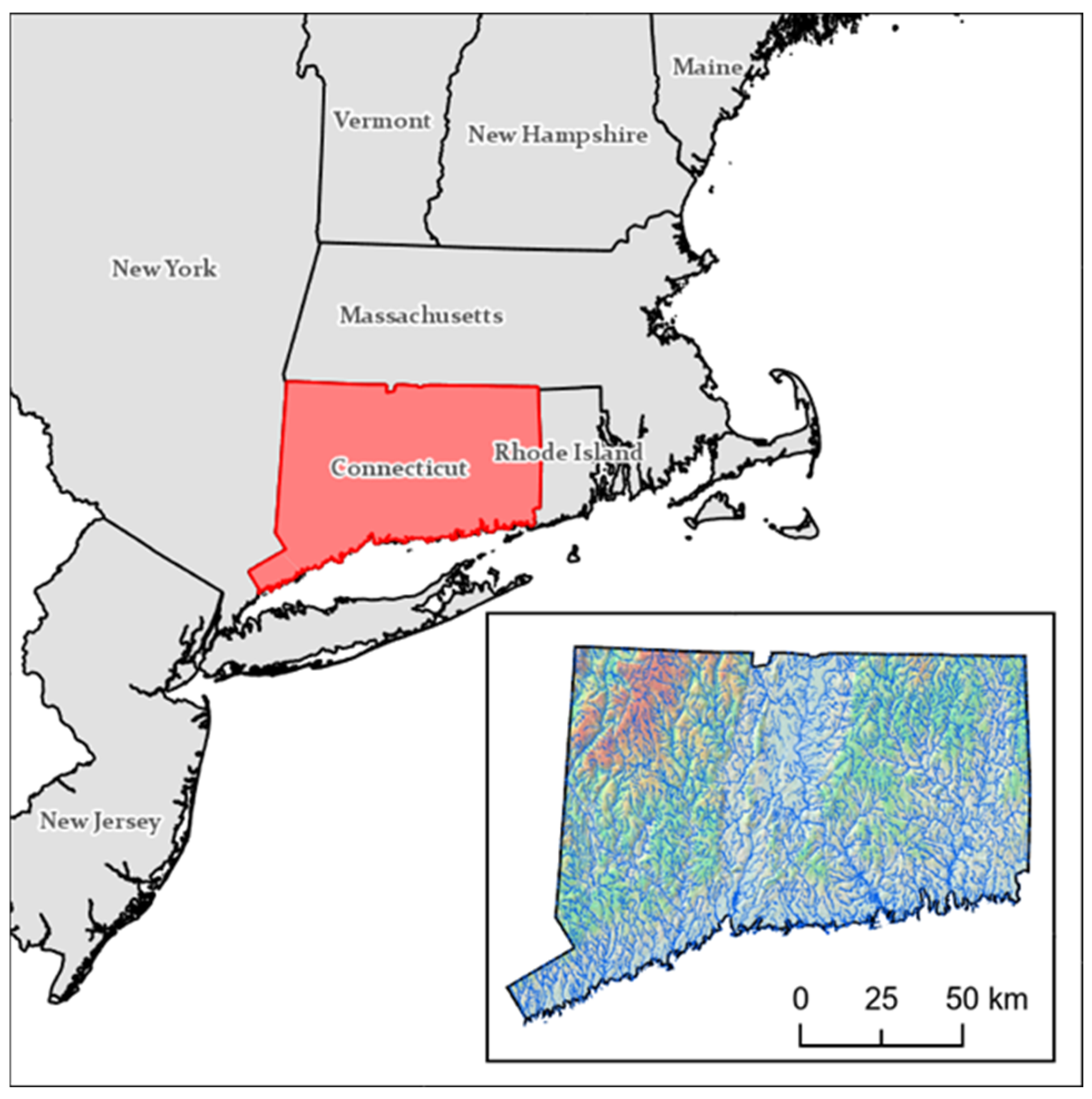
Figure 1. Map of the study area in Northeastern United States, highlighting the state of Connecticut (shaded in red). The inset map displays a hillshade elevation model of Connecticut overlaid with major river networks, illustrating the state’s varied topography and extensive hydrological features that contribute to habitat suitability for semi-aquatic species such as the beaver.
Ijgi 14 00383 g001
Figure 2. A generalized schematic of the beaver-influenced floodplain inundation modeling workflow. The workflow depicts the collection of training data images in the Data Collection/Preprocessing section. Collected images were fed into multiple deep learning configurations in the Deep Learning Ablation section. Using the highest-performing model, each type of training data type was used as training data in separate models. The highest-performing model and training data type was used to correct statewide temporal maps for Connecticut from 1990 to 2023.
Ijgi 14 00383 g002
Figure 3. Beaver habitat in Willington, Connecticut. (a) ~1 m resolution panchromatic aerial image acquired in 1990 under leaf-off condition (two beaver dams are shown as red line and yellow boxes); (b) ~0.7 m resolution multispectral aerial image acquired in 2016 under leaf-off condition (two beaver dams are shown in red); (b) Field photo of the same beaver habitat showing basic structural characteristics; (c) Zoomed-in view of the beaver lodge. Field photos were acquired in fall 2022.
Ijgi 14 00383 g003
Figure 4. A conceptual model of the beaver-influenced floodplain inundation (BIFI) (red crosshatch pattern). The model illustrates a spatially connected series of beaver ponds arranged in a cascading pattern along a stream network. BIFI represents the expansion of inundated floodplain area resulting from beaver dam construction, emphasizing the cumulative hydrological impact of multiple dams within a watershed. Edges throughout the BIFI are examined to show to edge of inundation.
Ijgi 14 00383 g004
Figure 5. Examples of beaver-influenced floodplain inundation (BIFI). (a) A spatially extensive BIFI spanning multiple overlapping aerial imagery tiles (red boxes), illustrating the cumulative effect of multiple beaver ponds across a broader floodplain. (b) A smaller, localized BIFI contained within a single image tile (red box), representing a more isolated beaver impact.
Ijgi 14 00383 g005
Figure 6. Distribution of the hand-annotated dataset across years and seasonal conditions. (a) Annual count of BIFI annotations from 1990 to 2019, categorized by image type and leaf condition: Panchromatic Leaf-off (blue), RGB Leaf-on (green), and RGB Leaf-off (yellow). (b) Proportion of total annotations by image type and leaf condition, highlighting the relative contribution of each imagery type to the full dataset.
Ijgi 14 00383 g006
Figure 7. Model architecture comparison using different encoder backbones and configurations across three segmentation architectures. (ad) SegFormer models with five encoder variants: B0-Finetuned, B1-Finetuned, B2-Finetuned, B3-Finetuned, and B4-Finetuned. (ei) U-Net++ models with four ResNet encoders: ResNet-18, ResNet-34, ResNet-50, and ResNet-101. (jn) YOLOv8-seg models with five configurations: YOLOv8n-seg, YOLOv8s-seg, YOLOv8m-seg, YOLOv8l-seg, and YOLOv8x-seg.
Ijgi 14 00383 g007aIjgi 14 00383 g007b
Figure 8. Training data ablation analysis comparing three imagery types, panchromatic leaf-off, RGB leaf-on, and RGB leaf-off. Each model is compared against the blended data model which is trained on the three imagery types. All models were trained using YOLOv8l-seg, which was the highest-performing model variant found in the ablation analysis.
Ijgi 14 00383 g008
Figure 9. Examples of straight-edge post-processing methodology (SEPM) correcting beaver-influenced floodplain inundation (BIFI) inferences: 2019 BIFI inference before SEPM (a); 2019 BIFI after SEPM (b); 2018 BIFI inference before SEPM (c); and 2018 BIFI after SEPM (d); Differences in BIFI inference count before and after SEPM is applied (e).
Ijgi 14 00383 g009
Figure 10. Inference count (a) and area (b) described over time annually. Winter (Leaf-off) and Summer (Leaf-on) years are differentiated for later discussion on the effects of occluded imagery on model performance.
Ijgi 14 00383 g010
Figure 11. Statewide beaver-influenced floodplain inundation density maps produced from 1990 (a) and 2019 (b) aerial images using the highest-performing YOLOv8l-seg model train. BIFI inferences were aggregated into 5 km2.
Ijgi 14 00383 g011
Figure 12. Beaver-influenced floodplain inundation inferences over the highest-performing models for each tested architecture (YOLOv8l-seg, U-Net++ ResNet-34, SegFormer B3-Finetuned). Inferences were made for three years; 1990 (panchromatic leaf-off), 2016 (RGB leaf-on), and 2019 (RGB leaf-off). For each year, true and false positive examples were found.
Ijgi 14 00383 g012aIjgi 14 00383 g012b
Figure 13. Beaver-influenced floodplain inundation inferences throughout Connecticut from 1990, 2004, and 2019. Four separate examples were present for each year with inferences in purple from the model. The first example (ac) identifies a BIFI where no beaver activity was present in 1990, and then a BIFI developed in 2004 and remained till 2019. The second example (df) identifies a BIFI where evidence of activity was present for each period and did not change in size. The third example (gi) identifies a BIFI where beaver activity was not present till 2004 but was not identified by the model. The fourth example (jl) shows a BIFI that was identified correctly, but the area increased then decreased over time.
Ijgi 14 00383 g013aIjgi 14 00383 g013b
Figure 14. RGB Leaf-on inferences using YOLOv8l-seg from 2018 imagery (a,d) is compared against RGB leaf-off inferences from 2019 (b,e) for two beaver-influenced floodplain inundations (purple) around Connecticut. Inferenced beaver-influenced floodplain inundation (BIFI) from RGB leaf-on (blue) and RGB leaf-off (red) imagery are shown in (c,f), respectively.
Ijgi 14 00383 g014
Figure 15. Inference quality assessment using the highest-performing YOLOv8l-seg model. Red regions represent outputs generated by the model. False positive at 75% confidence using panchromatic imagery (a). RGB leaf-on and RGB leaf-off imagery without false positive (b,c). False negative present in panchromatic leaf-off imagery (d). True positive present in RGB leaf-on and RGB leaf-off imagery (e,f). False positives present in panchromatic leaf-off (g), RGB leaf-on (h), and RGB leaf-off (i). False negative present in panchromatic leaf-off (j), RGB leaf-on (k), and RGB leaf-off (l).
Ijgi 14 00383 g015
Table 1. Summary of statewide historical and contemporary aerial imagery acquisitions for Connecticut from 1934 to 2019. The table includes key attributes for each dataset: acquisition year, leaf cycle at the time of capture, spatial resolution, georeferencing status, number and type of spectral bands, cloud cover, area imaged, data originators, and whether the imagery was utilized in this study.
Acquisition YearLeaf-On/OffSpatial Resolution (m)Georeferenced
(Yes/No)
Spectral BandsCloud CoverArea ImagedOriginatorsUsed in This Study?
1934Off1NPanchromaticn/aStatewideFairchild Aerial Survey, Inc. for the State Planning BoardNo
1951-52On1NPanchromaticn/aStatewideRobinson Aerial Surveys, Inc., for the U.S. Department of Agriculture, Agriculture Stabilization and Marketing ServiceNo
1965Off1NPanchromaticn/aStatewideKeystone Aerial Surveys, Inc., for the Department of Public WorksNo
1970Off1NPanchromaticn/aStatewideKeystone Aerial Survey, Inc. for the State Department of TransportationNo
1985-86Off1NPanchromaticn/aStatewideAero Graphics Corp., Bohemia, NYNo
1990Off1YPanchromaticn/aStatewideDEEP, U.S. Geological SurveyTraining
Inferencing
2004Off0.30YPanchromaticn/aStatewideDEEP, Aero-Metric, Inc.Training
Inferencing
2006On1YRGB10StatewideSDA-FSA-APFO Aerial Photography Field OfficeTraining
Inferencing
2008On1YRGB, NIR10StatewideUSDA-FSA-APFO Aerial Photography Field OfficeTraining
Inferencing
2010On1YRGB, NIR10StatewideUSDA-FSA-APFO Aerial Photography Field OfficeTraining
Inferencing
2012Off0.30YRGB, NIR0StatewidePhoto Science, State of Connecticut Department of Emergency Services and Public ProtectionTraining
Inferencing
2012On1YRGB, NIR10StatewideUSDA-FSA-APFO Aerial Photography Field OfficeTraining
Inferencing
2014On1YRGB, NIR10StatewideUSDA-FSA-APFO Aerial Photography Field OfficeTraining
Inferencing
2016Off0.08YRGB, NIR0StatewideThe Sanborn Map Company, State of Connecticut Department of Emergency Services and Public ProtectionTraining
Inferencing
2016On0.60YRGB, NIR10StatewideUSDA-FSA-APFO Aerial Photography Field OfficeTraining
Inferencing
2018On0.60YRGB, NIR10StatewideUSDA-FSA-APFO Aerial Photography Field OfficeTraining
Inferencing
2019Off0.15YRGB, NIR0StatewideQuantum Spatial Inc., State of Connecticut Department of Emergency Services and Public ProtectionTraining
Inferencing
2021On0.6YRGB, NIR-StatewideUSDA-FSA-APFO Aerial Photography Field OfficeInferencing
2023Off0.08YRGB, NIR-StatewideOffice of Policy and ManagementInferencing
2023On0.6YRGB, NIR-StatewideUSDA-FSA-APFO Aerial Photography Field OfficeNo
Table 2. All architecture combinations tested within the deep learning ablation to discover the highest-performing model combination for beaver-influenced floodplain inundation segmentation. Three different architectures, either semantic or instance, were paired with an encoder differing in the number of parameters.
ArchitectureModel VariantsParametersCitation
TransformerSemanticSegFormerB0-Finetuned3.4 MXie et al., 2021 [42]
SegFormerB1-Finetuned13.0 M
SegFormerB2-Finetuned25.0 M
SegFormerB3-Finetuned45.0 M
SegFormerB4-Finetuned60.0 M
Convolutional Neural NetsU-Net++ResNet-1811.7 MZhou et al., 2018 [43]
U-Net++ResNet-3421.8 M
U-Net++ResNet-5025.6 M
U-Net++ResNet-10144.6 M
InstanceYOLOv8YOLOv8n-Seg3.2 MUltralytics, 2023
YOLOv8YOLOv8s-Seg11.2 M
YOLOv8YOLOv8m-Seg25.9 M
YOLOv8YOLOv8l-Seg43.7 M
YOLOv8YOLOv8x-Seg68.2 M
Table 3. Results of model ablation study comparing three deep learning architectures with ten different encoder configurations. Performance metrics include precision, recall, F1-score, and Intersection over Union (IoU), recorded to evaluate segmentation accuracy across architectures and encoder variants.
ModelEpochsBIFI PrecisionBIFI RecallBIFI F1BIFI IoU
SegFormer B0-Finetuned610.64710.50810.52020.4191
SegFormer B1-Finetuned340.68980.68980.54250.4389
SegFormer B2-Finetuned340.69880.57530.58550.4825
SegFormer B3-Finetuned130.74170.69920.68340.5775
SegFormer B4-Finetuned140.69070.53920.55510.4527
U-Net++ ResNet-1890.80420.77060.76050.6650
U-Net++ ResNet-34290.81930.78860.78020.6942
U-Net++ ResNet-50220.79770.78280.75820.6628
U-Net++ ResNet-101160.80900.76330.75720.6625
YOLOv8n-seg420.77650.83500.78160.6983
YOLOv8s-seg570.79550.85500.80290.7225
YOLOv8m-seg200.79170.84860.79850.7211
YOLOv8l-seg250.79640.85770.80590.7259
YOLOv8x-seg210.79010.83420.79470.7210
Table 4. Pixel-based map accuracy results for Massachusetts Ipswich watershed and Oregon Umpqua watershed.
Ipswich, MAUmpqua River, Oregon
Percentage true positive3.250.00
Percentage false positive0.400.00
Percentage false negative0.650.10
Percentage true negative95.7099.90
Table 5. Inference analysis of Oregon Umpqua River watershed due to low density of beaver-influenced floodplain inundation in pixel-based map accuracy assessment.
Percentage true positive13.27
Percentage false positive86.73
Disclaimer/Publisher’s Note: The statements, opinions and data contained in all publications are solely those of the individual author(s) and contributor(s) and not of MDPI and/or the editor(s). MDPI and/or the editor(s) disclaim responsibility for any injury to people or property resulting from any ideas, methods, instructions or products referred to in the content.