Globally Optimal Relative Pose and Scale Estimation from Only Image Correspondences with Known Vertical Direction

Abstract

Installing multi-camera systems and inertial measurement units (IMUs) in self-driving cars, micro aerial vehicles, and robots is becoming increasingly common. An IMU provides the vertical direction, allowing coordinate frames to be aligned in a common direction. The degrees of freedom (DOFs) of the rotation matrix are reduced from 3 to 1. In this paper, we propose a globally optimal solver to calculate the relative poses and scale of generalized cameras with a known vertical direction. First, the cost function is established to minimize algebraic error in the least-squares sense. Then, the cost function is transformed into two polynomials with only two unknowns. Finally, the eigenvalue method is used to solve the relative rotation angle. The performance of the proposed method is verified on both simulated and KITTI datasets. Experiments show that our method is more accurate than the existing state-of-the-art solver in estimating the relative pose and scale. Compared to the best method among the comparison methods, the method proposed in this paper reduces the rotation matrix error, translation vector error, and scale error by 53%, 67%, and 90%, respectively.

1. Introduction

Estimating the relative pose from two views is a cornerstone in multi-view geometry problems which has been applied in many fields, such as visual odometry (VO) [1,2], structure from motion (SfM) [3,4], and simultaneous localization and mapping (SLAM) [5,6,7]. In addition, the camera sensor for indoor positioning is also an application [8,9,10]. The multi-camera system consists of multiple individual cameras fixed on a system. It has the advantages of a large field of view and high precision in relative pose estimation. Therefore, a large number of scholars have studied how to improve the accuracy, robustness, and efficiency of the relative pose estimation algorithm.

Compared with the standard pinhole camera, the multi-camera system lacks a single projection center. To solve this problem, Plücker lines are proposed to represent the light rays that pass through the multi-camera system [8]. This model is called the generalized camera model (GCM) [11], which describes the relationship between the Plücker lines and the generalized essential matrix. Generalized cameras are widely used in fields such as autonomous driving, robotics, and micro aerial vehicles. Pless proposed calculating the relative poses of multiple cameras using 17-point correspondences. Some methods have been developed on multi-camera relative pose estimation using the generic camera model [12,13,14,15,16,17]. However, these algorithms can estimate multi-camera poses only if the distances between all camera centers are known. This assumption limits the use of the generic camera model. In this paper, we focus on estimating the relative poses and scales of the generic camera model.

The relative pose and scale of the multi-camera system consist of a total of 7 degrees of freedom (DOFs), including 3 DOFs of the rotation matrix, 3 DOFs of translation vectors, and 1 DOF for scale, as shown in Figure 1. To improve the relative pose estimation of the camera and reduce the minimum number of required feature point pairs, an auxiliary sensor, such as an IMU, is often added [13,14,15,18,19,20]. An IMU can provide the yaw, pitch, and roll angles. The pitch and roll angles are more accurate than the yaw angle [21]. Therefore, we can use the pitch and roll angle provided by the IMU to reduce the degrees of freedom of the rotation matrix from 3 to 1. In this case, the relative pose and scale of the multi-camera system consist of a total of 5 degrees of freedom (DOFs). Thus, only five feature point pairs are needed to estimate the relative poses and scales of the camera [22].

Figure 1. The rotation matrix, translation vector, and scale are $R$, $t$, and $\mathrm{s}$, respectively.

Depending on the number of points required to solve the relative poses of a multi-camera system, solvers can be divided into minimum sample solvers and non-minimum sample solvers. When the distance between camera centers is known, a large number of scholars have used both minimum and non-minimum samples to solve for the relative poses of cameras. A constraint equation for the rotation matrix, translation vector, scale, and Plücker lines in the generic camera model is proposed in [22]. The minimum solution for a known vertical direction is also known. This method avoids 3D point noise in the calculation of relative poses and scale using the method with 2D-3D point correspondences. A simple heuristic global energy minimization scheme based on local minimum suppression is proposed in [23]. However, this method is not a closed-form solver.

This paper mainly focuses on globally optimal relative pose and scale estimation from 2D-2D point correspondences. Cameras and IMUs, such as mobile phones, unmanned aerial vehicles, and autonomous vehicles, are usually fixed together, so we assume the vertical direction is known. The main contributions of this paper are summarized below:

• A novel globally optimal solver to estimate relative pose and scale is proposed from N 2D-2D point correspondences (N > 5). This problem is transformed into a cost function based on the least-squares sense to minimize algebraic error.
• We transform the cost function to solve two unknowns in two equations, which are composed of the parameter of the relative rotation angle. The highest degree of rotation angle parameter is 16.
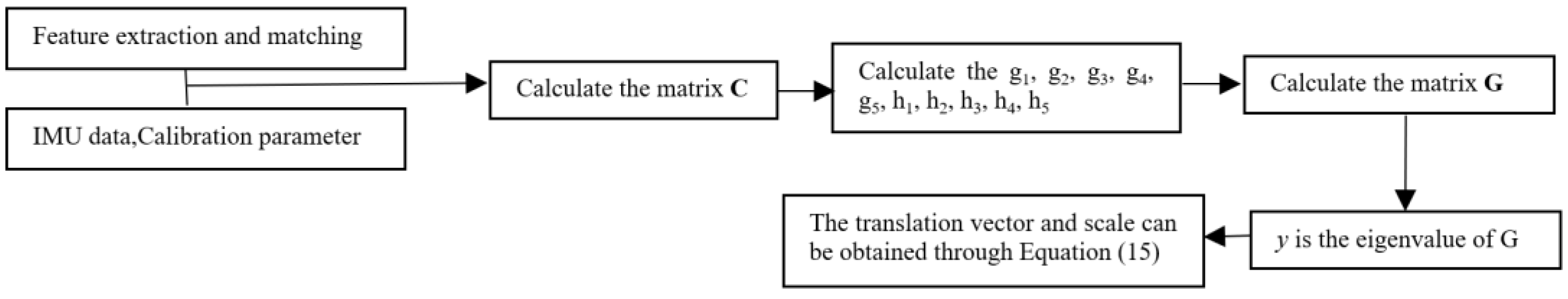
• We derive and provide a solver based on polynomial eigenvalues to calculate the relative rotation angle parameter. The translation vector and scale information are obtained from the corresponding eigenvectors.

The rest of this paper is organized as follows. We review the related work in Section 2. In Section 3, we introduce methodology, including the generalized epipolar constraint, problem description, and globally optional solver. We test the performance of the proposed method on synthetic and real-world data and discuss this in Section 4. The conclusions are presented in Section 5.

2. Related Work

Multi-camera relative pose estimation has received significant attention in academia and industry. The multi-camera model differs from the standard pinhole model due to the absence of a single center of projection in the multi-camera system.

Grossberg and Nayar introduced the generalized camera model [24]. To describe the lines sampled in space for each pixel in a multi-camera system, Pless proposed using Plücker lines to express light rays and provide the relationship between the Plücker vector, the rotation matrix, and the translation vector [11]. The generalized camera model proposed by Pless has been widely used in multi-cameras. Stewenius et al. proposed an estimation of the relative pose using six-point correspondences in a multi-camera system [12]. This solver generates 64 solutions using the Gröbner basis technique. However, this method runs slow when solving for relative pose. Li et al. proposed a linear solver using 17-point correspondences [16]. Based on this, Li et al. analyzed the degeneracy of the 17-point method and proposed a new solver [25]. Some solvers were proposed where the IMU provides the pitch angle and roll angle. Lee et al. proposed a solver to estimate the yaw angle by computing an eight-degree univariate polynomial using four-point correspondences [13]. Sweeney et al. transformed the relative pose estimation problem into a quadratic eigenvalue problem [15]. Liu also proposed the use of four-point correspondences to calculate the relative pose of the camera [14]. Guan et al. proposed four solutions using affine correspondences in a multi-camera system [26]. Kneip utilized the minimization of the algebraic error to build the objective function to solve the rotation matrix and then calculated the translation vector based on the eigenvalues and eigenvectors [17]. Zhao proposed a globally optimal solver by transforming the minimization of the sum of squares of residuals constructed from generalized epipolar constraints into quadratically constrained quadratic programming (QCQP) [27]. Ding proposed a novel globally optimal solver using polynomial eigenvalue when the vertical direction is known [18].

All of the above methods are based on the case where the internal scale between two multi-camera systems is known. However, the internal scale of each view is difficult to obtain or is ambiguous. So, it is necessary to estimate the scale information of the camera. Ventura et al. provided a minimal solver to estimate the absolute pose and scale of the generalized camera using four 2D-3D correspondences [24]. This solver produces eight solutions. Sweeney et al. proposed a globally optimal solver from four or more 2D-3D correspondences [28]. This method does not need iterations or initialization in the process of solving. The accuracy of pose and scale estimation using 2D-3D correspondence is greatly affected by the depth because this method relies on the accuracy of 3D. To reduce the influence of depth, some scholars propose using 2D-2D correspondence to calculate relative pose and scale.

Sweeney first proposed using 2D-2D correspondence to calculate the relative poses and scale between two generalized cameras. A constraint on the rotation matrix, translation vector, scale, and Plücker vector was presented. The authors provided two solvers (a quadratic eigenvalue solver and a closed-form solver) when the vertical direction is known based on five-point correspondences. Experiments showed that they are ill-conditioned and very unstable in quadratic eigenvalue solutions [22]. Kneip dropped the assumption of known vertical direction. Kneip transformed the relative pose and scale problem into a symmetric eigenvalue problem. The method computes the rotation matrix by direct search using a minimally suppressed heuristic global optimization method [23]. However, the method is not a closed-form solution. Recently, the solver of polynomial eigenvalue has been widely applied in the field of camera pose estimation [29,30,31,32].

3. Methodology

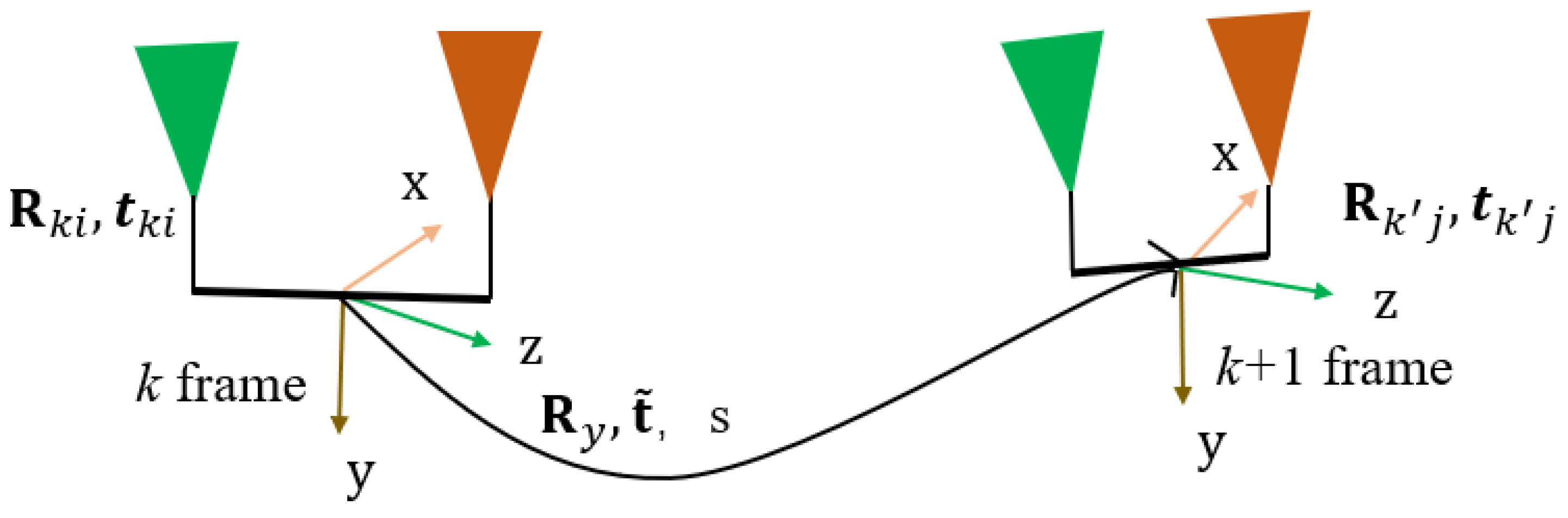
3.1. Epipolar Constraint

In a multi-camera system, we define a corresponding point pair $(x_{ki},x_{k^{\prime }j},R_{ki},R_{k^{\prime }j},t_{ki},t_{k^{\prime }j})$, where $x_{ki}$ is the normalized homogeneous coordinate of the $i$-th camera capture image in the $k$ frame and $x_{k^{\prime }j}$ is the normalized homogeneous coordinate of the $j$-th camera capture image in the $k+1$ frames. The rotation matrix and translation vector of the $i$-th camera in the $k$ frame are $R_{ki}$ and $t_{ki}$. The rotation matrix and translation vector of the $j$-th camera in the $k+1$ frame are $R_{k^{\prime }j}$ and $t_{k^{\prime }j}$ in Figure 2. $I_{ki}$ and $I_{k^{\prime }j}$ denote a pair of corresponding Plücker line vectors pointing at $k$ and $k+1$ frames. The Plücker line vector is written as follows:

$$I_{ki}=\left(\begin{array}{c}{f}_{ki}\\ t_{ki}\times f_{ki}\end{array}\right),\hspace{1em}{I}_{k^{\prime }j}=\left(\begin{array}{c}{f}_{k^{\prime }j}\\ t_{k^{\prime }j}\times f_{k^{\prime }j}\end{array}\right),$$

(1)

where $f_{ki}$ and $f_{k^{\prime }j}$ denote the direction vectors of the corresponding rays between the two generalized cameras. $f_{ki}$ and $f_{k^{\prime }j}$ are written as follows:

$$f_{ki}=\frac{(R_{ki}{x}_{ki})}{‖R_{ki}{x}_{ki}‖},\hspace{1em}\hspace{1em}{f}_{k^{\prime }j}=\frac{(R_{k^{\prime }j}{x}_{k^{\prime }j})}{‖R_{k^{\prime }j}{x}_{k^{\prime }j}‖}.$$

(2)

Figure 2. The rotation matrix and translation vector of the $i$-th camera in the $k$ frame are $R_{ki}$ and $t_{ki}$. The rotation matrix and translation vector of the $j$-th camera in the $k+1$ frame are $R_{k^{\prime }j}$ and $t_{k^{\prime }j}$. The rotation matrix, translation vector, and scale vector between aligned $k$ and $k+1$ are $R_y$, $\tilde{t}$, and $s$.

The generalized epipolar constraint is written as follows:

$$I_{k^{\prime }i}^T\left[\begin{array}{cc}E& R\\ R& 0\end{array}\right]I_{ki}=0,$$

(3)

where $R$ and $t$ represent the original rotation matrix and original translation vector, respectively. The essential matrix $E={\left[t\right]}_{\times }R$ and ${\left[t\right]}_{\times }$ represents the antisymmetric matrix of $t$.

$$f_{k^{\prime }j}^{T}E{f}_{ki}+f_{k^{\prime }j}^T(R{[t_{k^{\prime }j}]}_{\times }-{[t_{ki}]}_{\times }R)f_{ki}=0.$$

(4)

A large number of solvers have been proposed for this problem. The premise of applying these methods is then based on the assumption that scale information has been reconciled. In the application, the scale information is fuzzy, so the above methods are not available. Therefore, we mainly focus on the relative pose estimation when the scale is unknown. Equation (5) can be easily obtained according to Equation (4).

$$f_{k^{\prime }j}^{T}E{f}_{ki}+f_{k^{\prime }j}^T(Rs{[t_{k^{\prime }j}]}_{\times }-{[t_{ki}]}_{\times }R)f_{ki}=0,$$

(5)

where s represents the scale. Similar to Equation (3), Equation (5) can be expressed as follows:

$$I_{k^{\prime }j}^T\left[\begin{array}{cc}E& R\\ sR& 0\end{array}\right]I_{ki}=0.$$

(6)

A multi-camera system is usually coupled with the IMU, which can provide the roll (${\theta }_x$) and pitch (${\theta }_z$) angles. We define the Y-axis of the camera coordinate system to be parallel to the vertical direction, and the X-Z plane is orthogonal to the Y-axis. $R_{\mathrm{imu}}$ and $R_{\mathrm{imu}}^{\prime }$ are provided by the IMU at $k$ and $k+1$ frame, respectively.

$$R_{\mathrm{imu}}=R_x{R}_z,$$

(7)

where $R_x$ and $R_z$ can be written as follows:

$$R_x=\left[\begin{array}{ccc}1& 0& 0\\ 0& \cos \left({\theta }_x\right)& -\sin \left({\theta }_x\right)\\ 0& \sin \left({\theta }_x\right)& \cos \left({\theta }_x\right)\end{array}\right],\hspace{1em}\hspace{0.17em}{R}_z=\left[\begin{array}{ccc}\cos \left({\theta }_z\right)& -\sin \left({\theta }_z\right)& 0\\ \sin \left({\theta }_z\right)& \cos \left({\theta }_z\right)& 0\\ 0& 0& 1\end{array}\right].$$

(8)

The rotation matrix and translation vector between the aligned frames $k$ and $k+1$ are $R_y$ and $\tilde{t}$. The relationship between the original relative pose ($R$ and $t$) and the aligned relative pose ($R_y$ and $\tilde{t}$) can be expressed as follows:

$$R={(R_{\mathrm{imu}}^{\prime })}^T{R}_y{R}_{\mathrm{imu}},t={(R_{\mathrm{imu}}^{\prime })}^T\tilde{t},$$

(9)

where

$$R_y=\left[\begin{array}{ccc}\cos \left({\theta }_y\right)& 0& \sin \left({\theta }_y\right)\\ 0& 1& 0\\ -\sin \left({\theta }_y\right)& 0& \cos \left({\theta }_y\right)\end{array}\right],$$

(10)

where ${\theta }_y$ represents the rotation angle of the Y-axis. The rotation matrix $R_y$ can be rewritten with the Cayley parameterization as follows:

$$R_y=\frac{1}{1+y^2}\left[\begin{array}{ccc}1-y^2& 0& 2y\\ 0& 1& 0\\ -2y& 0& 1-y^2\end{array}\right],$$

(11)

where $y=\tan \frac{{\theta }_y}{2}$. In practical applications, ${\theta }_y$ = 180° is very rare [33].

By substituting Equation (9) into Equation (6), we can obtain

$${\left(\left[\begin{array}{cc}{R}_{\mathrm{imu}}^{\prime }& 0\\ 0& R_{\mathrm{imu}}^{\prime }\end{array}\right]I_{k^{\prime }j}\right)}^T\cdot \left[\begin{array}{cc}{\left[\tilde{t}\right]}_{\times }{R}_y& R_y\\ s{R}_y& 0\end{array}\right]\cdot \left(\left[\begin{array}{cc}{R}_{\mathrm{imu}}& 0\\ 0& R_{\mathrm{imu}}\end{array}\right]I_{ki}\right)=0.$$

(12)

By substituting Equation (1) into Equation (12), we can obtain

$${\left(\begin{array}{c}{R}_{\mathrm{imu}}^{\prime }{f}_{k^{\prime }j}\\ R_{\mathrm{imu}}^{\prime }(t_{k^{\prime }j}\times f_{k^{\prime }j})\end{array}\right)}^T\cdot \left[\begin{array}{cc}{\left[\tilde{t}\right]}_{\times }{R}_y& R_y\\ s{R}_y& 0\end{array}\right]\cdot \left(\begin{array}{c}{R}_{\mathrm{imu}}{f}_{ki}\\ R_{\mathrm{imu}}(t_{ki}\times f_{ki})\end{array}\right)=0.$$

(13)

3.2. Problem Description

Based on the constraint equation of Equation (13) in the previous section, Equation (13) can be rewritten as follows:

$${\underset{M}{\underbrace{\left(\begin{array}{c}{f}_{k^{\prime }j}\times {(R_{\mathrm{imu}}^{\prime })}^T{R}_y{R}_{\mathrm{imu}}{f}_{ki}\\ f_{k^{\prime }j}^T{\left[t_{k^{\prime }j}\right]}_{\times }{(R_{\mathrm{imu}}^{\prime })}^T{R}_y{R}_{\mathrm{imu}}{f}_{ki}\\ -f_{k^{\prime }j}^T{(R_{\mathrm{imu}}^{\prime })}^T{R}_y{R}_{\mathrm{imu}}\left[t_{ki}\right]f_{ki}\end{array}\right)}}}^T\left(\begin{array}{c}\tilde{t}\\ s\\ 1\end{array}\right)=0,$$

(14)

where the size of M is 5 × 1. Suppose there are N point correspondences. If $N=5$, Sweeney proposes the solver using 5-point correspondences in [22]. In this paper, we focus on non-minimal sample point correspondences ($N>5$). We can stack the constraints in each correspondence

$$M^T\left(\begin{array}{c}\tilde{t}\\ s\\ 1\end{array}\right)={(m_1\dots m_n)}^T\left(\begin{array}{c}\tilde{t}\\ s\\ 1\end{array}\right)=0,$$

(15)

We minimize the algebraic error based on the least-squares sense and establish the cost function

$${\arg }_{R_y,\tilde{t}}\min {\widehat{t}}^{T}C\widehat{t},$$

(16)

where $\widehat{t}={\left[\begin{array}{ccc}\tilde{t}& s& 1\end{array}\right]}^T$ and $C=M\times M^T$. Matrix C can be expressed as follows:

$$C=\left[\begin{array}{ccccc}{C}_{11}& C_{12}& C_{13}& C_{14}& C_{15}\\ C_{12}& C_{22}& C_{23}& C_{24}& C_{25}\\ C_{13}& C_{23}& C_{33}& C_{34}& C_{35}\\ C_{14}& C_{24}& C_{34}& C_{44}& C_{45}\\ C_{15}& C_{25}& C_{35}& C_{45}& C_{55}\end{array}\right].$$

(17)

The only unknown in matrix $C$ is $y$. Supposing ${\lambda }_{C,\min }$ is the smallest eigenvalue of matrix $C$, the optimization problem is expressed by

$$R_{\mathrm{y}}=\arg {\min }_{R_{\mathrm{y}}}{\lambda }_{C,\min }.$$

(18)

Based on the form of the eigenvalues, we can write

$$\det (C-\lambda I)=-{\lambda }^5+f_1{\lambda }^4+f_2{\lambda }^3+f_3{\lambda }^2+f_4\lambda +f_5,$$

(19)

where $\lambda$ is the eigenvalue of matrix $C$, and $I$ is a $5\times 5$ unit matrix. Specific expressions for $f_0$, $f_1$, $f_2$, $f_3$, and $f_4$ contain only the unknown $y$.

For convenience of narration, we use $\lambda$ instead of ${\lambda }_{G,\min }$. Based on the properties of eigenvalues, Equation (19) can be rewritten as follows:

$$-{\lambda }^5+f_1{\lambda }^4+f_2{\lambda }^3+f_3{\lambda }^2+f_4\lambda +f_5=0.$$

(20)

$\frac{\mathrm{d}\lambda }{\mathrm{d}s}=0$ is the necessary condition for $\lambda$ to be the smallest eigenvalue of $C$. We can obtain

$$\frac{d{f}_1}{d\lambda }{\lambda }^4+\frac{d{f}_2}{d\lambda }{\lambda }^3+\frac{d{f}_3}{d\lambda }{\lambda }^2+\frac{d{f}_4}{d\lambda }\lambda +\frac{d{f}_5}{d\lambda }=0.$$

(21)

Define $\alpha =1+y^2$. Then, we can obtain

$$f_1=\frac{g_1}{{\delta }^2},f_2=\frac{g_2}{{\delta }^4},f_3=\frac{g_3}{{\delta }^6},f_4=\frac{g_4}{{\delta }^7},f_5=\frac{g_5}{{\delta }^8},$$

(22)

$$\frac{d{f}_1}{dy}=\frac{h_1}{{\delta }^3},\frac{d{f}_2}{dy}=\frac{h_2}{{\delta }^5},\frac{d{f}_3}{dy}=\frac{h_3}{{\delta }^7},\frac{d{f}_4}{dy}=\frac{h_4}{{\delta }^8},\frac{d{f}_5}{dy}=\frac{h_5}{{\delta }^9},$$

(23)

where $g_1$, $g_2$, $g_3$, $g_4$, $g_5$, $h_1$, $h_2$, $h_3$, $h_4$, and $h_5$ are only polynomials of $y$. The highest degree of $y$ is shown in Table 1.

Table 1. Highest degree of variable $y$.

	${\mathit{g}}_1$	${\mathit{g}}_2$	${\mathit{g}}_3$	${\mathit{g}}_4$	${\mathit{g}}_5$	${\mathit{h}}_1$	${\mathit{h}}_2$	${\mathit{h}}_3$	${\mathit{h}}_4$	${\mathit{h}}_5$
Degree of $y$	4	8	12	14	16	4	8	12	14	16

Define $\beta =\delta \lambda$. Equations (20) and (21) can be rewritten as follows:

$$\left\{\begin{array}{l}-{\delta }^3{\beta }^5+{\delta }^2{\beta }^4{g}_1+\delta {\beta }^3{g}_2+{\beta }^2{g}_3+\beta g_4+g_5=0\hfill \\ {\delta }^2{\beta }^4{h}_1+\delta {\beta }^3{h}_2+{\beta }^2{h}_3+\beta h_4+h_5=0\hfill \end{array}\right..$$

(24)

We can rewrite Equation (24) as follows:

$$\left[\begin{array}{llllll}-{\delta }^3\hfill & {\delta }^2{g}_1\hfill & \delta g_2\hfill & g_3\hfill & g_4\hfill & g_5\hfill \\ 0\hfill & {\delta }^2{h}_1\hfill & \delta h_2\hfill & h_3\hfill & h_4\hfill & h_5\hfill \end{array}\right]\left[\begin{array}{l}{\beta }^5\hfill \\ {\beta }^4\hfill \\ {\beta }^3\hfill \\ {\beta }^2\hfill \\ \begin{array}{c}\beta \\ 1\end{array}\hfill \end{array}\right]=0.$$

(25)

3.3. Globally Optimal Solver

We can easily find two equations with 6 monomials in Equation (24). To equalize the number of equations and the number of monomials, the first equation of Equation (24) is equalized by ${\beta }^3$, ${\beta }^2$, and $\beta$, and the second equation is equalized by ${\beta }^4$, ${\beta }^3$, ${\beta }^2$, and $\beta$. We can obtain seven equations.

$$\left\{\begin{array}{l}-{\delta }^3{\beta }^6+{\delta }^2{\beta }^5{g}_1+\delta {\beta }^4{g}_2+{\beta }^3{g}_3+{\beta }^2{g}_4+\beta g_5=0\hfill \\ -{\delta }^3{\beta }^7+{\delta }^2{\beta }^6{g}_1+\delta {\beta }^5{g}_2+{\beta }^4{g}_3+{\beta }^3{g}_4+{\beta }^2{g}_5=0\hfill \\ -{\delta }^3{\beta }^8+{\delta }^2{\beta }^7{g}_1+\delta {\beta }^6{g}_2+{\beta }^5{g}_3+{\beta }^4{g}_4+{\beta }^3{g}_5=0\hfill \\ {\delta }^2{\beta }^5{h}_1+\delta {\beta }^4{h}_2+{\beta }^3{h}_3+{\beta }^2{h}_4+\beta h_5=0\hfill \\ {\delta }^2{\beta }^6{h}_1+\delta {\beta }^5{h}_2+{\beta }^4{h}_3+{\beta }^3{h}_4+{\beta }^2{h}_5=0\hfill \\ {\delta }^2{\beta }^7{h}_1+\delta {\beta }^6{h}_2+{\beta }^5{h}_3+{\beta }^4{h}_4+{\beta }^3{h}_5=0\hfill \\ {\delta }^2{\beta }^8{h}_1+\delta {\beta }^7{h}_2+{\beta }^6{h}_3+{\beta }^5{h}_4+{\beta }^4{h}_5=0\hfill \end{array}\right..$$

(26)

Based on Equations (24) and (26), we can easily obtain nine equations with nine monomials.

$$V_{9\times 9}{X}_{9\times 1}=0,$$

(27)

where $V$ is 9 × 9 and $X$ is 9 × 1.

$$V=\left(\begin{array}{ccccccccc}0& 0& 0& -{\delta }^3& {\delta }^2{g}_4& \delta g_3& g_2& g_1& g_0\\ 0& 0& -{\delta }^3& {\delta }^2{g}_4& \delta g_3& g_2& g_1& g_0& 0\\ 0& -{\delta }^3& {\delta }^2{g}_4& \delta g_3& g_2& g_1& g_0& 0& 0\\ -{\delta }^3& {\delta }^2{g}_4& \delta g_3& g_2& g_1& g_0& 0& 0& 0\\ 0& 0& 0& 0& {\delta }^2{h}_4& \delta h_3& h_2& h_1& h_0\\ 0& 0& 0& {\delta }^2{h}_4& \delta h_3& h_2& h_1& h_0& 0\\ 0& 0& {\delta }^2{h}_4& \delta h_3& h_2& h_1& h_0& 0& 0\\ 0& {\delta }^2{h}_4& \delta h_3& h_2& h_1& h_0& 0& 0& 0\\ {\delta }^2{h}_4& \delta h_3& h_2& h_1& h_0& 0& 0& 0& 0\end{array}\right),$$

(28)

$$X={\left[\begin{array}{lllllllll}{\beta }^8\hfill & {\beta }^7\hfill & {\beta }^6\hfill & {\beta }^5\hfill & {\beta }^4\hfill & {\beta }^3\hfill & {\beta }^2\hfill & \beta \hfill & 1\hfill \end{array}\right]}^T.$$

(29)

The elements of $V$ are univariate polynomials in $y$, and the highest degree of $y$ is 16. Equation (27) can be rewritten as follows:

$$(V_0+y{V}_1+\dots +y^{16}{V}_{16})X=0.$$

(30)

We define the matrix $B$, $J$, $L$.

$$B=\left[\begin{array}{cccc}0& I& \dots & 0\\ 0& 0& \dots & 0\\ \dots & \dots & \dots & I\\ -V_0& -V_1& \dots & -V_{15}\end{array}\right],J=\left[\begin{array}{cccc}I& 0& \dots & 0\\ 0& I& \dots & 0\\ \dots & \dots & \dots & 0\\ 0& 0& \dots & V_{16}\end{array}\right],L=\left[\begin{array}{l}X\hfill \\ yX\hfill \\ \dots \hfill \\ y^{15}X\hfill \end{array}\right].$$

(31)

Equation (30) can be rewritten as $BL=yJL$. The eigenvalue of $J^{-1}B$ is $y$. $J^{-1}B$ can be written as follows:

$$J^{-1}B=\left[\begin{array}{cccc}0& I& \dots & 0\\ 0& 0& \dots & 0\\ \dots & \dots & \dots & I\\ -V_{16}^{-1}{V}_0& -V_{16}^{-1}{V}_1& \dots & -V_{16}^{-1}{V}_{15}\end{array}\right].$$

(32)

where $V_0$, $V_1$, …, $V_{15}$ and $V_{16}$ are 9 × 9 matrices.

It is found that the matrix $V_{16}^{-1}$ is inaccurate because there are zero columns, resulting in $V_{16}$ being a singular matrix. Since $V_0$ is full rank, we define $z=\frac{1}{y}$, and Equation (30) can be rewritten as follows:

$$({\mathrm{z}}^{16}{V}_0+z^{15}{V}_1+z^{14}{V}_2+\dots +V_{16})X=0$$

(33)

where $z$ is the eigenvalue of matrix $G$.

$$G=\left[\begin{array}{cccc}0& I& \dots & 0\\ 0& 0& \dots & 0\\ \dots & \dots & \dots & I\\ -V_0^{-1}{V}_{16}& -V_0^{-1}{V}_{15}& \dots & -V_0^{-1}{V}_1\end{array}\right]$$

(34)

A method for reducing the size of the polynomial eigenvalue problem is proposed in [32]. Zero columns and corresponding zero rows of matrix $G$ are removed. The eigenvalues of matrix $G$ are calculated using Schur decomposition. The translation vector and scale can be obtained through Equation (15) when $y$ is known. The algorithm flow chart is shown in Figure 3.

Figure 3. Algorithm flow chart.

The method proposed in this paper is suitable for cameras and IMUs that are fixedly connected together. The specific steps of the algorithm are as follows: (1) The data input to the algorithm include feature point pairs, pitch and roll angles provided by the IMU, and calibration parameters. (2) Based on the input data, calculate the coefficients of each element of matrix C in Equation (17) with respect to the variable y. (3) Calculate g₁, g₂, g₃, g₄, g₅, h₁, h₂, h₃, h₄, and h₅ according to Equations (20)–(23). (4) Calculate matrix G according to Equation (34). (5) The eigenvalue of matrix G is the rotation parameter $y$, thus obtaining the rotation matrix. (6) The translation vector and scale are obtained by bringing the rotation matrix into Equation (15).

4. Experiments

In this section, we test the accuracy of the rotation matrix, translation vector, and scale on synthetic and real-world data. Since the solver proposed in this paper is a global optimization solver with a known vertical direction, we chose Sw [22] for comparison. The method proposed in this paper is called OURs.

$${\epsilon }_R=\arccos (\frac{\mathrm{trace}(R_{gt}{R}^T)-1}{2})$$

(35)

$${\epsilon }_t=2\frac{‖t_{gt}-t‖}{(‖t_{gt}‖+‖t‖)}$$

(36)

$${\epsilon }_{t,\mathrm{dir}}=\arccos \frac{t_{gt}^{T}t}{(‖t_{gt}‖+‖t‖)}$$

(37)

$${\epsilon }_s=\frac{|s-s_{gt}|}{s_{gt}}$$

(38)

where $R_{gt}$, $t_{gt}$, and $s_{gt}$ are the truth of rotation, translation, and scale, respectively. $R$, $t$, and $s$ are the evaluated values of rotation, translation, and scale, respectively.

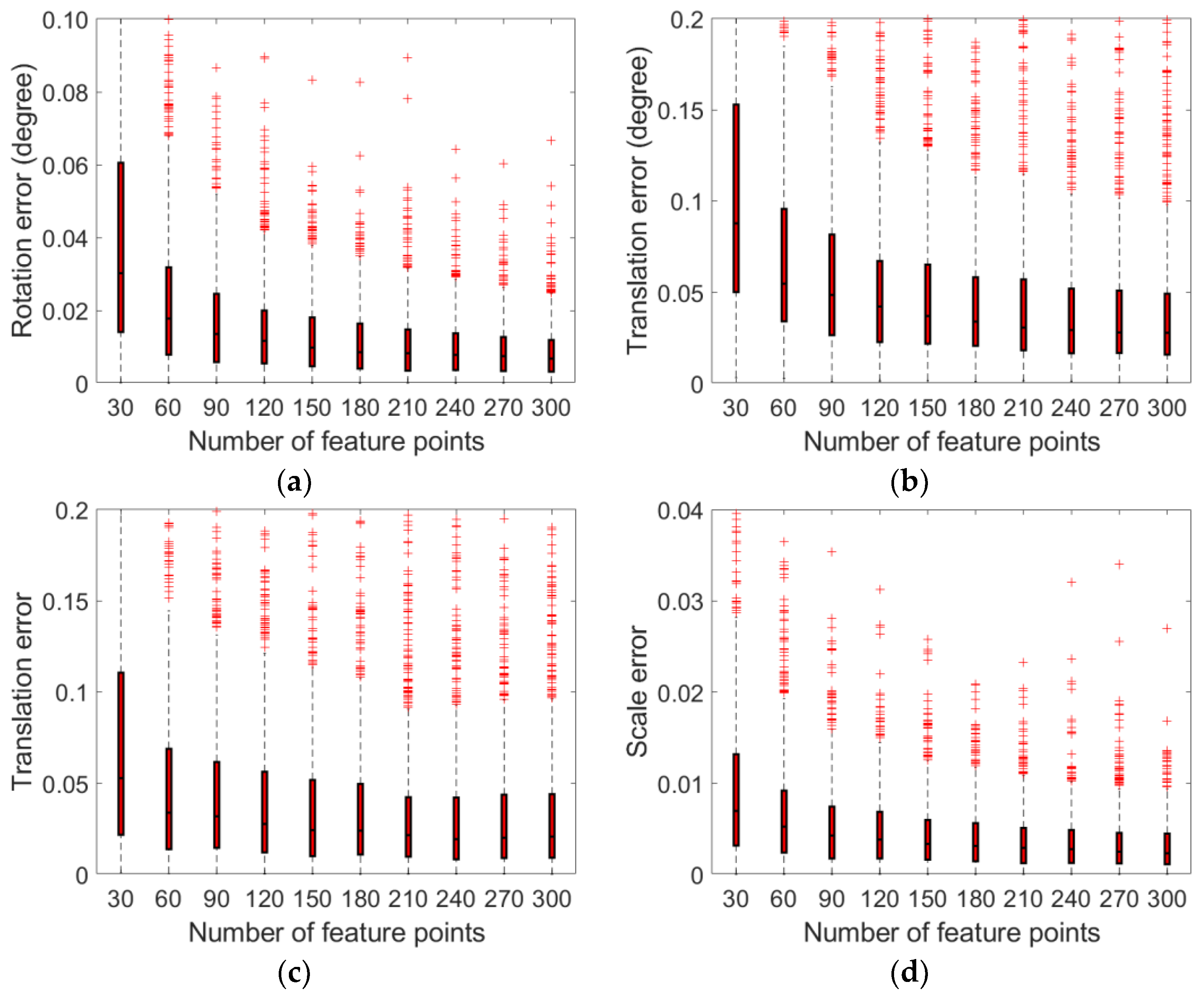
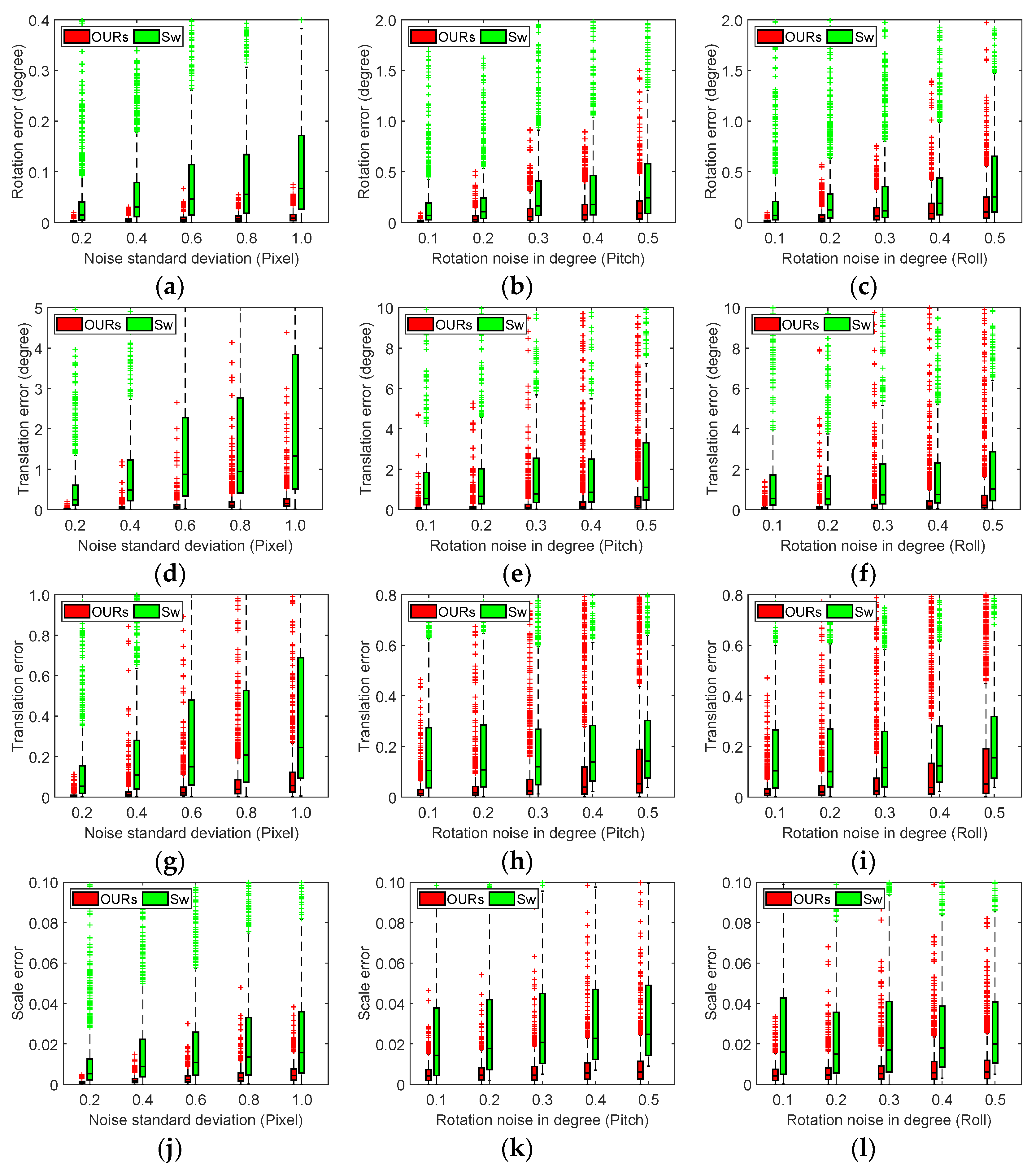
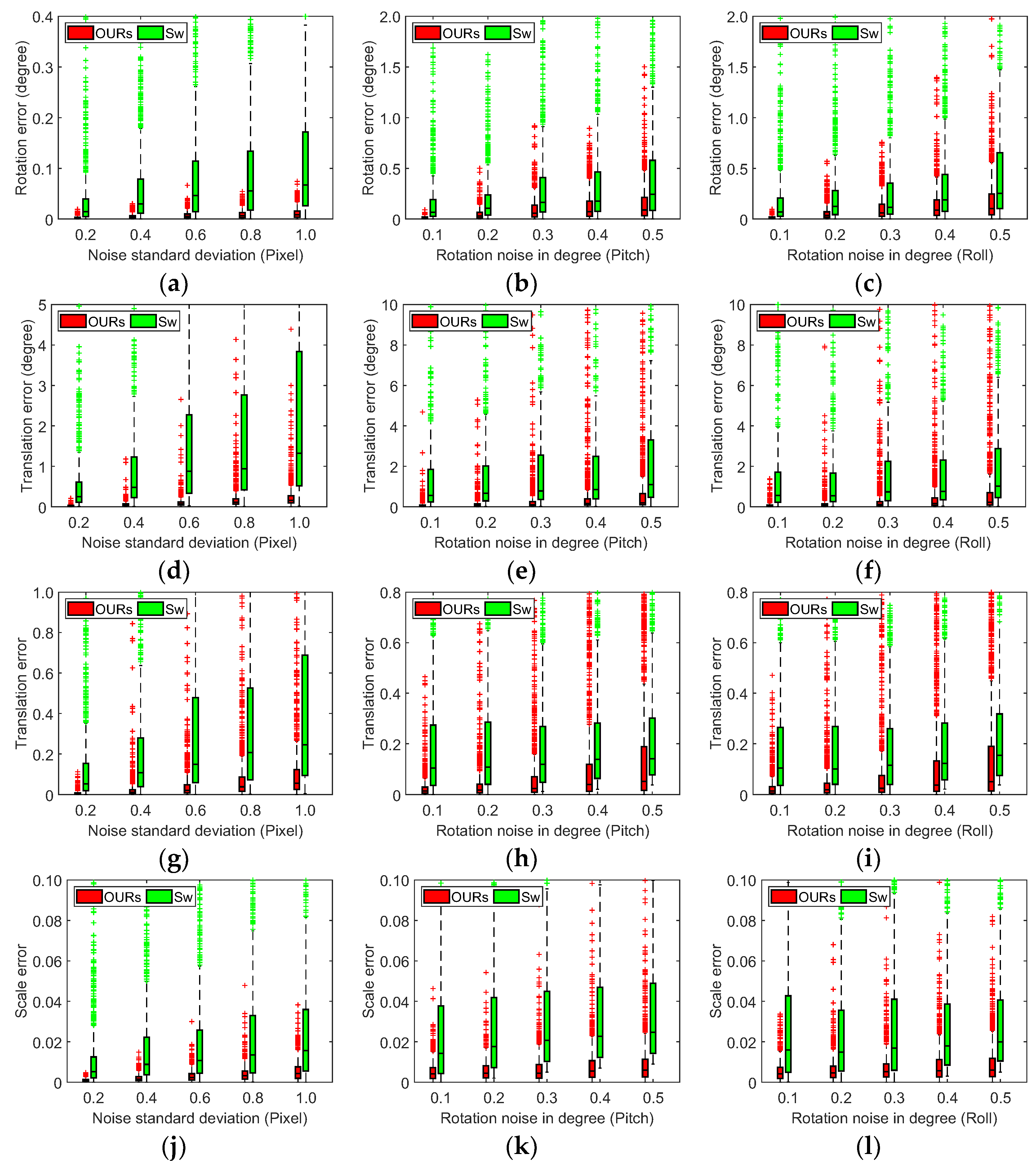
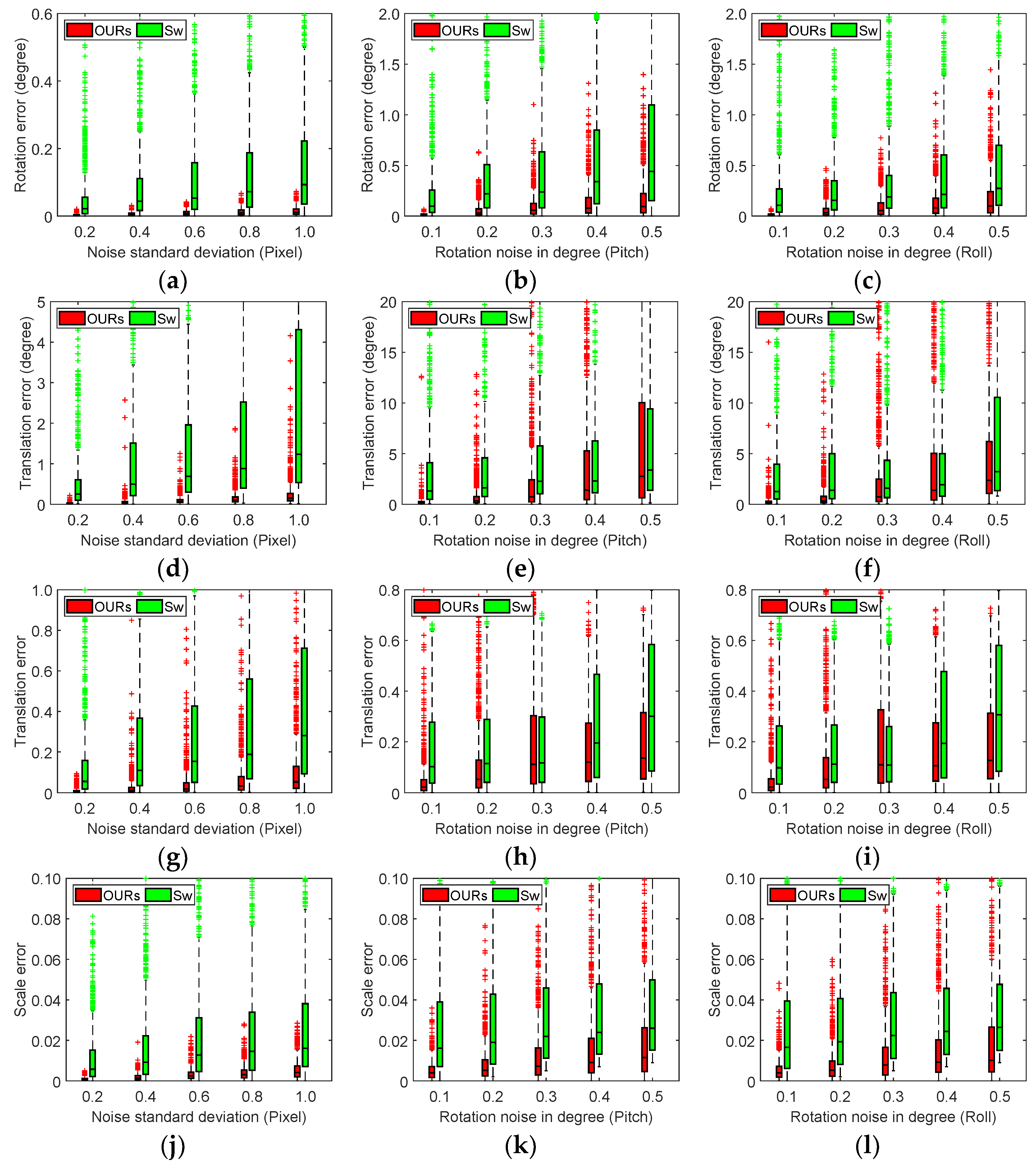
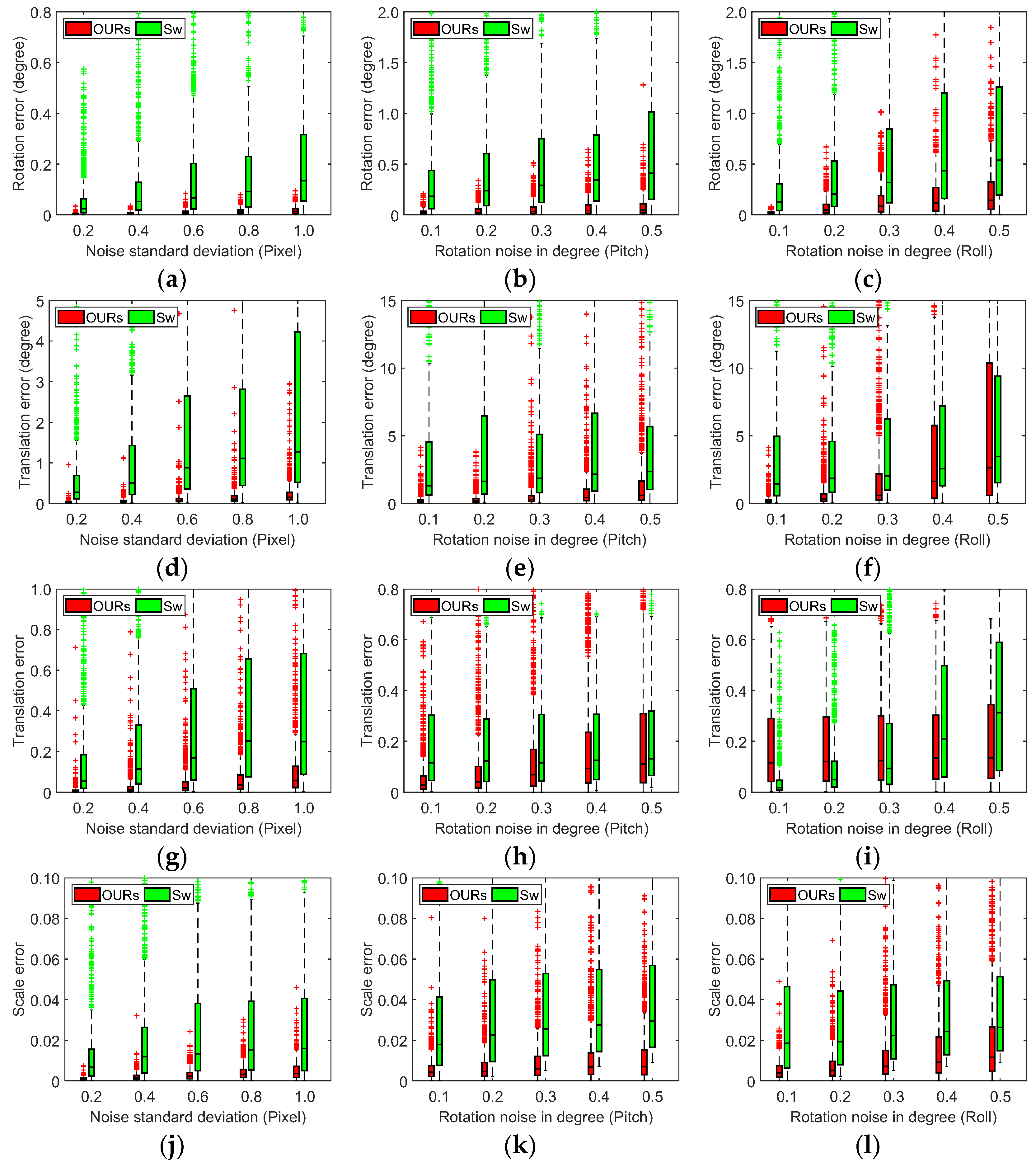
4.1. Experiments on Synthetic Data

To demonstrate the performance of the method proposed in this paper, we first perform experiments on a synthetic dataset. We randomly generate five cameras in space. Three hundred random 3D points are generated within a range of −5 to 5 m (X-axis), −5 to 5 m (Y-axis), and 5–20 m (Z-axis). The resolution of the image is 640 × 480 pixels, and the focal length of the camera is 400 pixels. We assume that the principal point is located at the center of the image at (320, 240) pixels. The scale $s$ is randomly generated in the range [0.5, 2]. Rotation matrices and translation vectors for the five cameras to the reference frame are randomly generated. We establish the frame of reference in the middle of the five cameras. The rotation angle between two adjacent reference frames ranges from −10° to 10°. The direction of the translation vector between two adjacent frames is also randomly generated, and the norm of the translation vector is between 1 and 2 m.

Parameter sensitivity analysis: Due to the fact that the solver proposed in this paper uses a non-minimum sample to estimate the relative pose of the camera and scale, we analyze the accuracy of the calculation by varying the number of points. We set the noise in the image to 1 pixel. The noise of the pitch angle and the noise of the roll angle are both zero degrees. Figure 4 shows the accuracy of rotation, translation, and scale estimation by OURs with different numbers of feature points. It is evident that as the number of points increases, the rotation error, translation error, and scale error estimated by the OURs method all decrease in Figure 4.

Figure 4. Effect of the number of feature points on the accuracy of rotation, translation, and scale estimation by the method proposed in this paper with different feature points. (a) Rotation error (degree); (b) translation error (degree); (c) translation error; (d) scale error.

Noise resilience: The solvers of Sw and OURs are tested with added image noise under four motions: random motion ($t={\left[\begin{array}{ccc}{t}_x& t_y& t_z\end{array}\right]}^T$), planar motion ($t={\left[\begin{array}{ccc}{t}_x& 0& t_z\end{array}\right]}^T$), forward motion ($t={\left[\begin{array}{ccc}0& 0& t_z\end{array}\right]}^T$), and sideways motion ($t={\left[\begin{array}{ccc}{t}_x& 0& 0\end{array}\right]}^T$). We add image noise ranging from 0 to 1 pixel. We added noise to the pitch angle and roll angle when adding noise to the IMU in the synthetic data. The noise of the image is fixed to 1 pixel when noise is added to the roll angle and pitch angle. The maximum noise of the roll angle and pitch angle is 0.5 degrees. Figure 5 shows the error values of the rotation matrix, translation vector, and scale calculated by OURs and Wu when the image noise, pitch angle noise, and roll angle are added under random motion. Figure 6 shows the error values of the rotation matrix, translation vector, and scale calculated by OURs and Wu when the image noise, pitch angle noise, and roll angle are added under planar motion. Figure 7 shows the error values of the rotation matrix, translation vector, and scale calculated by OURs and Wu when the image noise, pitch angle noise, and roll angle are added under sideways motion. Figure 8 shows the error values of the rotation matrix, translation vector, and scale calculated by OURs and Sw when the image noise, pitch angle noise, and roll angle are added under forward motion. The second column shows the calculation results of adding pitch angle noise. The third column shows the calculation results of adding roll angle noise. The first row represents the rotation matrix error. The second and third rows represent translation vector errors. The fourth row represents scale error. From Figure 5, Figure 6, Figure 7 and Figure 8, it can be observed that the method proposed in this paper yields rotation matrix errors, translation vector errors, and scale errors smaller than those estimated by the Sw method. The effectiveness of the proposed method is demonstrated through simulated data.

Figure 5. Estimating errors in the rotation matrix, translation vector, and scale information under random motion. The first column shows the calculation results of adding image noise. The second column shows the calculation results of adding pitch angle noise. The third column shows the calculation results of adding roll angle noise. The first, second, third and fourth rows represent the values of ${\epsilon }_R$, ${\epsilon }_t$, ${\epsilon }_{t,\mathrm{dir}}$ and ${\epsilon }_s$ respectively.

Figure 6. Estimating errors in the rotation matrix, translation vector, and scale information under planar motion. The first column shows the calculation results of adding image noise. The second column shows the calculation results of adding pitch angle noise. The third column shows the calculation results of adding roll angle noise. The first, second, third and fourth rows represent the values of ${\epsilon }_R$, ${\epsilon }_t$, ${\epsilon }_{t,\mathrm{dir}}$ and ${\epsilon }_s$ respectively.

Figure 7. Estimating errors in the rotation matrix, translation vector, and scale information under sideways motion. The first column shows the calculation results of adding image noise. The second column shows the calculation results of adding pitch angle noise. The third column shows the calculation results of adding roll angle noise. The first, second, third and fourth rows represent the values of ${\epsilon }_R$, ${\epsilon }_t$, ${\epsilon }_{t,\mathrm{dir}}$ and ${\epsilon }_s$ respectively.

Figure 8. Estimating errors in the rotation matrix, translation vector, and scale information under forward motion. The first column shows the calculation results of adding image noise. The second column shows the calculation results of adding pitch angle noise. The third column shows the calculation results of adding roll angle noise. The first, second, third and fourth rows represent the values of ${\epsilon }_R$, ${\epsilon }_t$, ${\epsilon }_{t,\mathrm{dir}}$ and ${\epsilon }_s$ respectively.

Random motion: When the image noise is 1 pixel, the average rotation matrix error calculated by the OURs method is 0.011°, with a median of 0.008° and a standard deviation of 0.010. The average rotation matrix error calculated by the Sw method is 0.197°, with a median of 0.06° and a standard deviation of 0.559. The average translation vector error calculated by the OURs method is 0.249°, with a median of 0.156° and a standard deviation of 0.374. The average translation vector error calculated by the Sw method is 6.927°, with a median of 1.323° and a standard deviation of 14.908. The average scale error calculated by the OURs method is 0.005, with a median of 0.004 and a standard deviation of 0.005. The average scale error calculated by the Sw method is 0.031, with a median of 0.015 and a standard deviation of 0.050. When the pitch noise is 0.5°, the average rotation matrix error calculated by the OURs method is 0.164°, with a median of 0.089° and a standard deviation of 0.224. The average rotation matrix error calculated by the Sw method is 0.624°, with a median of 0.245° and a standard deviation of 1.321. The average translation vector error calculated by the OURs method is 1.397°, with a median of 0.196° and a standard deviation of 4.239. The average translation vector error calculated by the Sw method is 5.562°, with a median of 1.099° and a standard deviation of 12.152. The average scale error calculated by the OURs method is 0.010, with a median of 0.006 and a standard deviation of 0.014. The average scale error calculated by the Sw method is 0.045, with a median of 0.025 and a standard deviation of 0.068. When the roll noise is 0.5°, the average rotation matrix error calculated by the OURs method is 0.183°, with a median of 0.103° and a standard deviation of 0.230. The average rotation matrix error calculated by the Sw method is 0.591°, with a median of 0.253° and a standard deviation of 1.136. The average translation vector error calculated by the OURs method is 2.051°, with a median of 0.221° and a standard deviation of 8.799. The average translation vector error calculated by the Sw method is 5.595°, with a median of 1.021° and a standard deviation of 12.733. The average scale error calculated by the OURs method is 0.010, with a median of 0.006 and a standard deviation of 0.012. The average scale error calculated by the Sw method is 0.037, with a median of 0.019 and a standard deviation of 0.052.

Planar motion: When the image noise is 1 pixel, the average rotation matrix error calculated by the OURs method is 0.015°, with a median of 0.012° and a standard deviation of 0.013. The average rotation matrix error calculated by the Sw method is 0.368°, with a median of 0.097° and a standard deviation of 1.134. The average translation vector error calculated by the OURs method is 0.194°, with a median of 0.093° and a standard deviation of 0.722. The average translation vector error calculated by the Sw method is 4.864°, with a median of 0.802° and a standard deviation of 12.211. The average scale error calculated by the OURs method is 0.005, with a median of 0.004 and a standard deviation of 0.005. The average scale error calculated by the Sw method is 0.0374, with a median of 0.016 and a standard deviation of 0.069. When the pitch noise is 0.5°, the average rotation matrix error calculated by the OURs method is 0.127°, with a median of 0.071° and a standard deviation of 0.156. The average rotation matrix error calculated by the Sw method is 0.883°, with a median of 0.357° and a standard deviation of 1.644. The average translation vector error calculated by the OURs method is 4.802°, with a median of 0.838° and a standard deviation of 11.473. The average translation vector error calculated by the Sw method is 7.813°, with a median of 1.847° and a standard deviation of 14.928. The average scale error calculated by the OURs method is 0.015, with a median of 0.008 and a standard deviation of 0.019. The average scale error calculated by the Sw method is 0.049, with a median of 0.030 and a standard deviation of 0.059. When the roll noise is 0.5°, the average rotation matrix error calculated by the OURs method is 0.156°, with a median of 0.090° and a standard deviation of 0.182. The average rotation matrix error calculated by the Sw method is 0.931°, with a median of 0.353° and a standard deviation of 1.897. The average translation vector error calculated by the OURs method is 5.271°, with a median of 1.006° and a standard deviation of 12.505. The average translation vector error calculated by the Sw method is 6.234°, with a median of 1.762° and a standard deviation of 12.573. The average scale error calculated by the OURs method is 0.019, with a median of 0.008 and a standard deviation of 0.020. The average scale error calculated by the Sw method is 0.046, with a median of 0.026 and a standard deviation of 0.065.

Sideways motion: When the image noise is 1 pixel, the average rotation matrix error calculated by the OURs method is 0.015°, with a median of 0.011° and a standard deviation of 0.012. The average rotation matrix error calculated by the Sw method is 0.295°, with a median of 0.093° and a standard deviation of 0.797. The average translation vector error calculated by the OURs method is 0.250°, with a median of 0.151° and a standard deviation of 0.373. The average translation vector error calculated by the Sw method is 6.638°, with a median of 1.231° and a standard deviation of 13.752. The average scale error calculated by the OURs method is 0.005, with a median of 0.004 and a standard deviation of 0.005. The average scale error calculated by the Sw method is 0.0374, with a median of 0.016 and a standard deviation of 0.076. When the pitch noise is 0.5°, the average rotation matrix error calculated by the OURs method is 0.160°, with a median of 0.094° and a standard deviation of 0.185. The average rotation matrix error calculated by the Sw method is 1.019°, with a median of 0.441° and a standard deviation of 1.708. The average translation vector error calculated by the OURs method is 9.559°, with a median of 2.765° and a standard deviation of 17.419. The average translation vector error calculated by the Sw method is 9.693°, with a median of 3.385° and a standard deviation of 15.701. The average scale error calculated by the OURs method is 0.020, with a median of 0.012 and a standard deviation of 0.024. The average scale error calculated by the Sw method is 0.044, with a median of 0.026 and a standard deviation of 0.058. When the roll noise is 0.5°, the average rotation matrix error calculated by the OURs method is 0.169°, with a median of 0.099° and a standard deviation of 0.198. The average rotation matrix error calculated by the Sw method is 0.732°, with a median of 0.274° and a standard deviation of 1.365. The average translation vector error calculated by the OURs method is 8.354°, with a median of 2.348° and a standard deviation of 12.123. The average translation vector error calculated by the Sw method is 10.764°, with a median of 3.230° and a standard deviation of 19.194. The average scale error calculated by the OURs method is 0.020, with a median of 0.010 and a standard deviation of 0.026. The average scale error calculated by the Sw method is 0.045, with a median of 0.026 and a standard deviation of 0.062.

Forward motion: When the image noise is 1 pixel, the average rotation matrix error calculated by the OURs method is 0.016°, with a median of 0.013° and a standard deviation of 0.015. The average rotation matrix error calculated by the Sw method is 0.421°, with a median of 0.135° and a standard deviation of 1.215. The average translation vector error calculated by the OURs method is 0.321°, with a median of 0.149° and a standard deviation of 1.325. The average translation vector error calculated by the Sw method is 7.156°, with a median of 1.27° and a standard deviation of 15.035. The average scale error calculated by the OURs method is 0.005, with a median of 0.004 and a standard deviation of 0.005. The average scale error calculated by the Sw method is 0.036, with a median of 0.016 and a standard deviation of 0.068. When the pitch noise is 0.5°, the average rotation matrix error calculated by the OURs method is 0.082°, with a median of 0.048° and a standard deviation of 0.104. The average rotation matrix error calculated by the Sw method is 0.965°, with a median of 0.411° and a standard deviation of 1.614. The average translation vector error calculated by the OURs method is 2.195°, with a median of 0.589° and a standard deviation of 5.921. The average translation vector error calculated by the Sw method is 9.442°, with a median of 2.364° and a standard deviation of 17.648. The average scale error calculated by the OURs method is 0.012, with a median of 0.007 and a standard deviation of 0.015. The average scale error calculated by the Sw method is 0.049, with a median of 0.029 and a standard deviation of 0.060. When the roll noise is 0.5°, the average rotation matrix error calculated by the OURs method is 0.229°, with a median of 0.141° and a standard deviation of 0.260. The average rotation matrix error calculated by the Sw method is 1.068°, with a median of 0.537° and a standard deviation of 1.639. The average translation vector error calculated by the OURs method is 11.024°, with a median of 2.628° and a standard deviation of 22.204. The average translation vector error calculated by the Sw method is 9.431°, with a median of 3.476° and a standard deviation of 14.699. The average scale error calculated by the OURs method is 0.020, with a median of 0.012 and a standard deviation of 0.024. The average scale error calculated by the Sw method is 0.046, with a median of 0.026 and a standard deviation of 0.068.

4.2. Experiments on Real-World Data

To further validate the effectiveness of the proposed method, the KITTI dataset was chosen for real data evaluation [31]. The KITTI dataset was jointly founded by the Karlsruhe Institute of Technology in Germany and the Toyota American Institute of Technology. It is currently the largest computer vision algorithm evaluation dataset in the world for autonomous driving scenarios. The raw dataset is divided into the categories ‘Road’, ‘City’, ‘Residential’, ‘Person’, and ‘Campus’. The car is equipped with GPS, an IMU, one 64-line 3D LiDAR, and two grayscale cameras. The KITTI dataset provides ground truth for 11 sequences (00–10). The pitch angle and roll angle can be extracted from the IMU sensor data. The intrinsic parameters of the camera and the rotation and translation between two cameras from the reference frame are given in the data document [34]. We utilized the SIFT algorithm to obtain corresponding feature point pairs. Figure 8 shows the results of feature extraction and matching using SIFT in the KITTI dataset. We selected one out of every five pairs of points for display in Figure 9.

Figure 9. Test image pair from KITTI dataset with feature detection.

Table 2 shows the error results of the rotation matrix, translation vector, and scale estimated by the OURs method and the Sw method on the KITTI dataset. From Table 2, we can see that the accuracy of the rotation matrix, translation vector, and scale estimated by the OURs method is significantly better than that of the Sw method. Table 3 shows the percentage by which the error calculated by the OURs method is reduced compared to the error calculated by the Sw method. For the rotation matrix, the OURs method computes the error on average about 53% less than the Sw method. The maximum error of the OURs method decreased by 71%, and the minimum decreased by 32%. For the translation vector, the OURs method computes the error on average about 67% less than the Sw method. The maximum error of the OURs method decreased by 73%, and the minimum decreased by 61%. For the scale, the OURs method computes the error on average about 90% less than the Sw method. The maximum error of the OURs method decreased by 95%, and the minimum decreased by 80%. The standard deviation of the rotation matrix estimated by the OURs method is 65% less than that of the Sw method. The standard deviation of the translation vector estimated by the OURs method is 51% less than that of the Sw method. The standard deviation of the scale estimated by the OURs method is 94% less than that of the Sw method.

Table 2. Rotation, translation, and scale error on KITTI sequence by the Sw method and the OURs method.

Seq	Sw			OURs
	${\mathit{\epsilon }}_{\mathbf{R}}$ (Degree)	${\mathit{\epsilon }}_{\mathbf{t},\mathbf{dir}}$ (Degree)	${\mathit{\epsilon }}_{\mathit{s}}$	${\mathit{\epsilon }}_{\mathbf{R}}$ (Degree)	${\mathit{\epsilon }}_{\mathbf{t},\mathbf{dir}}$ (Degree)	${\mathit{\epsilon }}_{\mathit{s}}$
00	0.1760	3.4598	0.0086	0.0847	1.3452	0.0012
01	0.2509	4.1682	0.0205	0.1042	1.5081	0.0008
02	0.1985	3.9163	0.0096	0.0965	1.2836	0.0010
03	0.1809	3.8168	0.0134	0.0754	1.0739	0.0009
04	0.1026	3.6274	0.0033	0.0590	1.0030	0.0003
05	0.2723	4.0362	0.0160	0.0801	1.2315	0.0008
06	0.1814	3.0784	0.0063	0.0664	1.0562	0.0003
07	0.0945	3.4602	0.0043	0.0452	1.1856	0.0008
08	0.1219	3.9419	0.0059	0.0833	1.0837	0.0012
09	0.2093	3.7111	0.0128	0.1133	1.2027	0.0011
10	0.1984	3.6022	0.0110	0.0864	1.3294	0.0008
AVG	0.1806	3.7107	0.0101	0.0813	1.2094	0.0008
MAX	0.2723	4.1682	0.0205	0.1133	1.5081	0.0012
MIN	0.0945	3.0784	0.0033	0.0452	1.0030	0.0003
SD	0.0537	0.2964	0.0050	0.0187	0.1443	0.0002
RMSE	0.1884	3.7225	0.0113	0.0835	1.2179	0.0008

Table 3. The percentage by which the error calculated by the OURs method is reduced compared to the error calculated by the Sw method.

Seq	Rotation (%)	Translation (%)	Scale (%)
00	52%	61%	86%
01	58%	64%	96%
02	51%	67%	90%
03	58%	72%	93%
04	42%	72%	91%
05	71%	69%	95%
06	63%	65%	95%
07	52%	66%	81%
08	32%	73%	80%
09	46%	68%	91%
10	56%	63%	93%
AVG	53%	67%	90%
MIN	32%	61%	80%
MAX	71%	73%	95%
SD	65%	51%	94%
RMSE	56%	67%	92%

To further verify the performance of the proposed method, we add the Kneip method [23], which is the latest method for estimating relative pose and scale from 2D-2D only without the use of an IMU. This method solves the relative pose and scale by using the non-minimum sample number. This method requires at least eight-point correspondences. The Kneip method transforms relative pose and scale estimation into a symmetric eigenvalue problem. A simple heuristic global energy minimization scheme based on local minimum suppression is used in the Kneip method. We added the Peter method [35], which requires a minimum of three 3D-3D correspondences to find the similarity. This is the orthogonal Procrustes approach. The 3D points are obtained by triangulating in each view.

Table 4 shows the rotation matrix errors, translation vector errors, and scale errors calculated by the Kneip method and the Peter method. As can be seen from Table 4, the average value, maximum value, minimum value, standard deviation, and root mean square error of the rotation matrix error estimated by the Kneip method are 0.8052°, 1.0643°, 0.5956°, 0.1340, and 0.8163. The average value, maximum value, minimum value, standard deviation, and root mean square error of the translation vector error estimated by the Kneip method are 5.1662°, 6.4101°, 4.2787°, 0.5699, and 5.1975. The average value, maximum value, minimum value, standard deviation, and root mean square error of the scale error estimated by the Kneip method are 0.0509, 0.0957, 0.0131, 0.0322, and 0.0603. The average value, maximum value, minimum value, standard deviation, and root mean square error of the rotation matrix error estimated by the Peter method are 1.8892°, 2.0592°, 1.7606°, 0.0894, and 1.8913. The average value, maximum value, minimum value, standard deviation, and root mean square error of the translation vector error estimated by the Peter method are 6.7648°, 9.8001°, 5.2621°, 1.2423, and 6.8779. The average value, maximum value, minimum value, standard deviation, and root mean square error of the scale error estimated by the Peter method are 0.0963, 0.1254, 0.0712, 0.0180, and 0.0979.

Table 4. Rotation, translation, and scale error on KITTI sequence by the Kneip method and the Peter method.

Seq	Kneip			Peter
	${\mathit{\epsilon }}_{\mathbf{R}}$ (Degree)	${\mathit{\epsilon }}_{\mathbf{t},\mathbf{dir}}$ (Degree)	${\mathit{\epsilon }}_{\mathit{s}}$	${\mathit{\epsilon }}_{\mathbf{R}}$ (Degree)	${\mathit{\epsilon }}_{\mathbf{t},\mathbf{dir}}$ (Degree)	${\mathit{\epsilon }}_{\mathit{s}}$
00	0.9147	6.4101	0.0204	1.9805	9.8001	0.0712
01	0.7057	5.0460	0.0913	1.7606	7.0888	0.1064
02	0.6269	4.9256	0.0258	1.8166	5.9685	0.0918
03	0.7856	4.9410	0.0835	1.8242	6.0235	0.1123
04	0.7901	4.7540	0.0298	1.7948	5.4217	0.0852
05	0.9512	6.0975	0.0957	1.9278	7.6275	0.1254
06	0.7506	4.2787	0.0277	1.9023	5.2621	0.0902
07	0.5956	5.0482	0.0157	1.7452	7.6125	0.0725
08	0.7816	5.1886	0.0130	1.8722	7.2626	0.0806
09	0.8919	5.2186	0.0816	1.9985	6.1282	0.1235
10	0.9643	4.9204	0.0758	2.0592	6.2176	0.1002
AVG	0.8052	5.1662	0.0509	1.8892	6.7648	0.0963
MAX	1.0643	6.4101	0.0957	2.0592	9.8001	0.1254
MIN	0.5956	4.2787	0.0131	1.7606	5.2621	0.0712
SD	0.1340	0.5699	0.0322	0.0894	1.2423	0.0180
RMSE	0.8163	5.1975	0.0603	1.8913	6.8779	0.0979

4.3. Discussion

The method proposed in this paper estimates the relative pose (4 DOFs) and scale from image correspondences. Therefore, the Sw method was chosen as the comparison method for the simulation experiment. From Figure 4, Figure 5, Figure 6 and Figure 7, it can be observed that the method proposed in this paper yields rotation matrix errors, translation vector errors, and scale errors smaller than those estimated by the Sw method. The effectiveness of the proposed method is demonstrated through simulated data. In the experiment on real data, to further verify the performance of the proposed method, we added the Kneip method and Peter method as comparison methods. The errors of the rotation matrix, translation vector, and scale calculated by our method are all smaller than those of the comparison method. The root mean square error of the rotation matrix estimated by the OURs method is 56% less than that of the Sw method. The root mean square error of the rotation matrix estimated by the OURs method is 90% less than that of the Kneip method. The root mean square error of the rotation matrix estimated by the OURs method is 96% less than that of the Peter method. The root mean square error of the translation vector estimated by the OURs method is 67% less than that of the Sw method. The root mean square error of the translation vector estimated by the OURs method is 77% less than that of the Kneip method. The root mean square error of the translation vector estimated by the OURs method is 82% less than that of the Peter method. The root mean square error of the scale estimated by the OURs method is 92% less than that of the Sw method. The root mean square error of the scale estimated by the OURs method is 98% less than that of the Kneip method. The root mean square error of the scale estimated by the OURs method is 99% less than that of the Peter method.

5. Conclusions

We propose a new globally optimal solver to estimate the relative pose and scale for a multi-camera system from only image correspondences with a known vertical direction. Firstly, we transformed the problem into a cost function based on the least-squares sense to minimize algebraic error. Based on the characteristic equation method and its first derivative equal to zero, two independent polynomial equations with two unknowns are provided. These two equations consist of the rotation angle parameter. We utilized the polynomial eigenvalue method to solve the rotation angle parameter. The translation vector and scale information were obtained based on the corresponding eigenvectors. We tested the superiority of the proposed method in relative pose and scale estimation on synthetic data and the KITTI dataset. Compared to the best method in the comparison methods, the method proposed in this paper reduced the rotation matrix error, translation vector error, and scale error by 53%, 67%, and 90%, respectively.

From Equation (14), it can be observed that the error sources of the proposed algorithm mainly come from the accuracy of feature extraction and matching, as well as the accuracy of the IMU. The measurement accuracy of the IMU is determined by the gyroscope. Our next task is to study how to enhance the accuracy of feature extraction and matching.

References

1. Zhang, J.; Xu, L.; Bao, C. An Adaptive Pose Fusion Method for Indoor Map Construction. ISPRS Int. J. Geo-Inf. 2021, 10, 800. [Google Scholar] [CrossRef]
2. Svärm, L.; Enqvist, O.; Kahl, F.; Oskarsson, M. City-scale localization for cameras with known vertical direction. IEEE Trans. Pattern Anal. Mach. Intell. 2016, 39, 1455–1461. [Google Scholar] [CrossRef] [PubMed]
3. Li, C.; Zhou, L.; Chen, W. Automatic Pose Estimation of Uncalibrated Multi-View Images Based on a Planar Object with a Predefined Contour Model. ISPRS Int. J. Geo-Inf. 2016, 5, 244. [Google Scholar] [CrossRef]
4. Raposo, C.; Barreto, J.P. Theory and practice of structure-from-motion using affine correspondences. In Proceedings of the IEEE Conference on Computer Vision and Pattern Recognition, Las Vegas, NV, USA, 27–30 June 2016; pp. 5470–5478. [Google Scholar]
5. Wang, Y.; Liu, X.; Zhao, M.; Xu, X. VIS-SLAM: A Real-Time Dynamic SLAM Algorithm Based on the Fusion of Visual, Inertial, and Semantic Information. ISPRS Int. J. Geo-Inf. 2024, 13, 163. [Google Scholar] [CrossRef]
6. Qin, J.; Li, M.; Liao, X.; Zhong, J. Accumulative Errors Optimization for Visual Odometry of ORB-SLAM2 Based on RGB-D Cameras. ISPRS Int. J. Geo-Inf. 2019, 8, 581. [Google Scholar] [CrossRef]
7. Mur-Artal, R.; Tardós, J.D. SLAM2: An open-source SLAM system for monocular, stereo, and RGB-D cameras. IEEE Trans. Robot 2017, 33, 1255–1262. [Google Scholar] [CrossRef]
8. Niu, Q.; Li, M.; He, S.; Gao, C.; Gary Chan, S.H.; Luo, X. Resource-efficient and Automated Image-based Indoor Localization. ACM Trans. Sens. Netw. 2019, 15, 19. [Google Scholar] [CrossRef]
9. Poulose, A.; Han, D.S. Hybrid Indoor Localization on Using IMU Sensors and Smartphone Camera. Sensors 2019, 19, 5084. [Google Scholar] [CrossRef] [PubMed]
10. Kawaji, H.; Hatada, K.; Yamasaki, T.; Aizawa, K. Image-based indoor positioning system: Fast image matching using omnidirectional panoramic images. In Proceedings of the 1st ACM International Workshop on Multimodal Pervasive Video Analysis, Firenze, Italy, 25–29 October 2010. [Google Scholar]
11. Pless, R. Using many cameras as one. In Proceedings of the IEEE Computer Society Conference on Computer Vision and Pattern Recognition, Madison, WI, USA, 18–20 June 2003; Volume 2, p. II-587. [Google Scholar]
12. HenrikStewénius, M.O.; Aström, K.; Nistér, D. Solutions to minimal generalized relative pose problems. In Proceedings of the Workshop on Omnidirectional Vision, Beijing, China, October 2005. [Google Scholar]
13. Hee Lee, G.; Pollefeys, M.; Fraundorfer, F. Relative pose estimation for a multi-camera system with known vertical direction. In Proceedings of the IEEE Conference on Computer Vision and Pattern Recognition, Columbus, OH, USA, 23–28 June 2014; pp. 540–547. [Google Scholar]
14. Liu, L.; Li, H.; Dai, Y.; Pan, Q. Robust and efficient relative pose with a multi-camera system for autonomous driving in highly dynamic environments. IEEE Trans. Intell. Transp. 2017, 19, 2432–2444. [Google Scholar] [CrossRef]
15. Sweeney, C.; Flynn, J.; Turk, M. Solving for relative pose with a partially known rotation is a quadratic eigenvalue problem. In Proceedings of the 2014 2nd International Conference on 3D Vision, Tokyo, Japan, 8–11 December 2014; Volume 1, pp. 483–490. [Google Scholar]
16. Li, H.; Hartley, R.; Kim, J. A linear approach to motion estimation using generalized camera models. In Proceedings of the IEEE Conference on Computer Vision and Pattern Recognition, Anchorage, AK, USA, 23–28 June 2008; pp. 1–8. [Google Scholar]
17. Kneip, L.; Li, H. Efficient computation of relative pose for multi-camera systems. In Proceedings of the IEEE Conference on Computer Vision and Pattern Recognition, Columbus, OH, USA, 23–28 June 2014; pp. 446–453. [Google Scholar]
18. Wu, Q.; Ding, Y.; Qi, X.; Xie, J.; Yang, J. Globally optimal relative pose estimation for multi-camera systems with known gravity direction. In Proceedings of the International Conference on Robotics and Automation, Philadelphia, PA, USA, 23–27 May 2022; pp. 2935–2941. [Google Scholar]
19. Guan, B.; Zhao, J.; Barath, D.; Fraundorfer, F. Minimal cases for computing the generalized relative pose using affine correspondences. In Proceedings of the IEEE/CVF International Conference on Computer Vision, Montreal, QC, Canada, 10–17 October 2021; pp. 6068–6077. [Google Scholar]
20. Guan, B.; Zhao, J.; Barath, D.; Fraundorfer, F. Relative pose estimation for multi-camera systems from affine correspondences. arXiv 2020, arXiv:2007.10700v1. [Google Scholar]
21. Kukelova, Z.; Bujnak, M.; Pajdla, T. Closed-form solutions to minimal absolute pose problems with known vertical direction. In Proceedings of the Asian Conference on Computer Vision, Queenstown, New Zealand, 8–12 November 2010; pp. 216–229. [Google Scholar]
22. Sweeney, C.; Kneip, L.; Hollerer, T.; Turk, M. Computing similarity transformations from only image correspondences. In Proceedings of the TEEE Conference on Computer Vision and Pattern Recognition, Boston, MA, USA, 7–12 June 2015; pp. 3305–3313. [Google Scholar]
23. Kneip, L.; Sweeney, C.; Hartley, R. The generalized relative pose and scale problem: View-graph fusion via 2D-2D registration. In Proceedings of the 2016 IEEE Winter Conference on Applications of Computer Vision, Lake Placid, NY, USA, 7–10 March 2016; pp. 1–9. [Google Scholar]
24. Grossberg, M.D.; Nayar, S.K. A general imaging model and a method for finding its parameters. In Proceedings of the Eighth IEEE International Conference on Computer Vision, Vancouver, BC, Canada, 7–14 July 2001; Volume 2, pp. 108–115. [Google Scholar]
25. Kim, J.H.; Li, H.; Hartley, R. Motion estimation for nonoverlap multicamera rigs: Linear algebraic and L∞ geometric solutions. IEEE Trans. Pattern Anal. Mach. Intell. 2009, 32, 1044–1059. [Google Scholar]
26. Guan, B.; Zhao, J.; Barath, D.; Fraundorfer, F. Minimal solvers for relative pose estimation of multi-camera systems using affine correspondences. Int. J. Comput. Vision 2023, 131, 324–345. [Google Scholar] [CrossRef]
27. Zhao, J.; Xu, W.; Kneip, L. A certifiably globally optimal solution to generalized essential matrix estimation. In Proceedings of the IEEE/CVF Conference on Computer Vision and Pattern Recognition, Seattle, WA, USA, 13–19 June 2020; pp. 12034–12043. [Google Scholar]
28. Sweeney, C.; Fragoso, V.; Höllerer, T.; Turk, M. gdls: A scalable solution to the generalized pose and scale problem. In Proceedings of the 13th European Conference, Zurich, Switzerland, 6–12 September 2014; pp. 16–31. [Google Scholar]
29. Bujnak, M.; Kukelova, Z.; Pajdla, T. 3d reconstruction from image collections with a single known focal length. In Proceedings of the IEEE 12th International Conference on Computer Vision, Kyoto, Japan, 29 September–2 October 2009; pp. 1803–1810. [Google Scholar]
30. Fitzgibbon, A.W. Simultaneous linear estimation of multiple view geometry and lens distortion. In Proceedings of the 2001 IEEE Computer Society Conference on Computer Vision and Pattern Recognition, Kauai, HI, USA, 8–14 December 2001; Volume 1, p. I. [Google Scholar]
31. Ding, Y.; Yang, J.; Kong, H. An efficient solution to the relative pose estimation with a common direction. In Proceedings of the 2020 IEEE International Conference on Robotics and Automation, Paris, France, 31 May–31 August 2020; pp. 11053–11059. [Google Scholar]
32. Kukelova, Z.; Bujnak, M.; Pajdla, T. Polynomial eigenvalue solutions to minimal problems in computer vision. IEEE Trans. Pattern Anal. Mach. Intell. 2011, 34, 1381–1393. [Google Scholar] [CrossRef]
33. Larsson, V.; Astrom, K.; Oskarsson, M. Efficient solvers for minimal problems by syzygy-based reduction. In Proceedings of the IEEE Conference on Computer Vision and Pattern Recognition, Honolulu, HI, USA, 21–26 July 2017; pp. 820–829. [Google Scholar]
34. Geiger, A.; Lenz, P.; Stiller, C.; Urtasun, R. Vision meets robotics: The kitti dataset. Int. J. Robot Res. 2013, 32, 1231–1237. [Google Scholar] [CrossRef]
35. Schonemann, P. A generalized solution of the orthogonal Procrustes problem. Psychometrika 1966, 31, 1–10. [Google Scholar] [CrossRef]
Disclaimer/Publisher’s Note: The statements, opinions and data contained in all publications are solely those of the individual author(s) and contributor(s) and not of MDPI and/or the editor(s). MDPI and/or the editor(s) disclaim responsibility for any injury to people or property resulting from any ideas, methods, instructions or products referred to in the content.
Article Metrics
Citations
Article Access Statistics
Multiple requests from the same IP address are counted as one view.