Abstract
This paper presents a comprehensive review of the accessibility measures and models used in land use and transportation planning, highlighting their evolution and recent applications. It categorizes the accessibility measures into passive and active, detailing their theoretical foundations and examining the differences between behavioral and non-behavioral models. By synthesizing the literature, this paper proposes a conceptual classification framework that integrates various accessibility measures. We aim to provide a structured classification of the accessibility measures, dividing them into various levels and grouping them into macro-areas and methodologies. This approach allows for the adaptation of the accessibility measures based on the specific study context, considering the hypotheses made beforehand and the relevant parameters for different scenarios. The findings emerging from the proposed classification framework highlight two opposite ways to measure accessibility: on the one hand, by considering the physical distance between locations, in terms of both spatial separation and proximity; on the other hand, by capturing individuals’ preferences and attitudes toward reaching goods, services or activities and then measuring the “perceived” accessibility. We underscore the necessity of considering both approaches in planning processes to create equitable and sustainable urban environments. This structured classification aims to guide researchers and planners in selecting appropriate tools tailored to specific contexts and needs, which means choosing the most appropriate accessibility measure to use, depending on the characteristics of the case being examined and the specific needs of the project.
1. Introduction
Tobler’s first law of geography (1970) easily expresses the spatial dependence between places and human activities by which “everything is related to everything else, but near things are more related than distant things”. This principle, known as distance decay, underlines the importance of proximity in any spatial interaction study. An important contribution to spatial analysis was made in 1820 by von Thünen, who explored the distribution of human activities to determine the optimal location for facilities, depending on the effective interaction with job, market and residential places. The relationship between transportation and the spatial development of cities has been systematically examined starting from the 1950s. The analysis of travel distances, density of locations and frequencies of travel was key to understanding and bounding urban sprawl. Land-use studies, applied to commercial, industrial, or residential areas, are in fact instrumental in determining the functional fabric of cities, shaping the landscape where diverse human activities unfold.
Every developing city necessitates specific planning of transport systems to bridge efficiently locations and facilities. Following this path, accessibility has been defined in many ways. Hansen [1] defined accessibility as a “measure of opportunities for spatial interactions” created by the distribution of transport systems, whereas Ben-Akiva and Lerman [2] defined it as “the benefits provided by a transportation land-use system” [3], p. 2.
A well-mapped distribution of accessibility can result in beneficial and accurate planning, favoring efficient resource allocation and the development of initiatives within some areas. The interaction between private choices in the transportation system, which shape the accessibility of both single neighborhoods and extended areas, and the land uses of territories may be represented by a feedback cycle [4]. This means that the measure of accessibility is particularly sensitive to the balance between demand and supply, i.e., to alterations within the land-use system (e.g., urbanization and congestion of specific areas) in response to users’ utilization of opportunities, such as different available modal choices. Therefore, alterations in the service levels within a wider area will affect the accessibility of single places and enhance or decrease the presence of opportunities in specific locations, affecting the accessibility from any other destination.
The observation of the regularities of specific parameters has led to mathematical models used to fit, at best, the distribution of travel frequencies. In a broader context, the frequencies are often proportional to the sizes of locations and inversely proportional to the travel costs, expressed as the disutility for the user, such as the travel time, distance or ease of running away, posing an analogy with Newton gravitational law. Accessibility is then an index representing the closeness of a specific area to all other activities in a region and, reasoning based on the literal meaning of the word, evaluating accessibility means assessing how a system or an environment allows users to interact with services or relevant areas.
Over the years, accessibility has been evaluated using different approaches, some of which are based on mathematics and physics, others on social and economic studies, making it possible to classify the measures according to conceptual assumptions.
Some relevant reviews and acknowledgments have meant organizing or grouping different kinds of measures, in most cases agreeing on a general framework of methodologies. As Ingram [5] identified two main types of indicators, integral measures and relative measures, Morris et al. [6] divided the integral ones into spatial separation measures and composite measures, these last ones leading to potential types. Baradaran and Ramjerdi [7] listed a set of five approaches: travel cost approach, gravity or opportunity approach, constraints-based approach, utility-based approach, and composite approach. Geurs and van Wee [8] looked at four main accessibility measures: infrastructure-based, location-based, utility-based, and person-based measures. Cascetta et al. [9,10] focused instead on the differences between behavioral and non-behavioral models, both analyzed from the aggregate and disaggregate points of view, for the case of cost-based and opportunity-based models.
2. Materials and Methods
Starting from the previously reviewed accessibility measures, we try to find a link between them and so to build a conceptual map (Figure 1, Figure 2 and Figure 3). The models will be specified, showing subsequent cases of study.

Figure 1.
Conceptual map of the accessibility measures reviewed from the literature. Main division into active measures and passive measures.

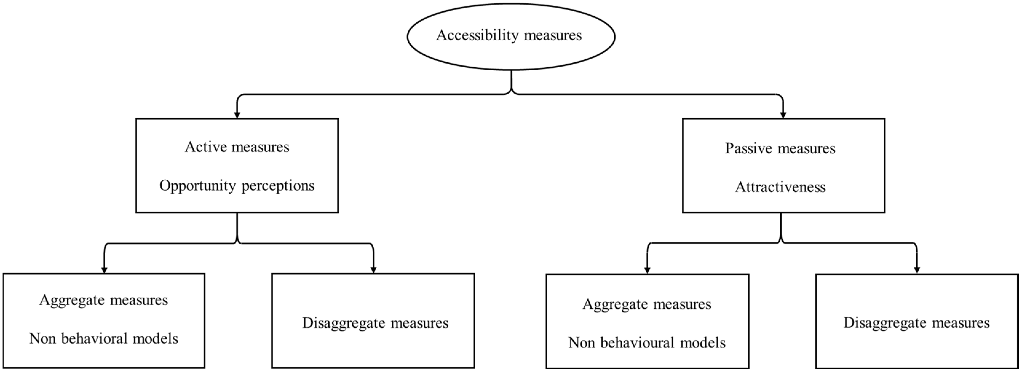
Figure 2.
Conceptual map of the accessibility measures reviewed from the literature. Description of passive measures.
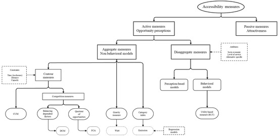
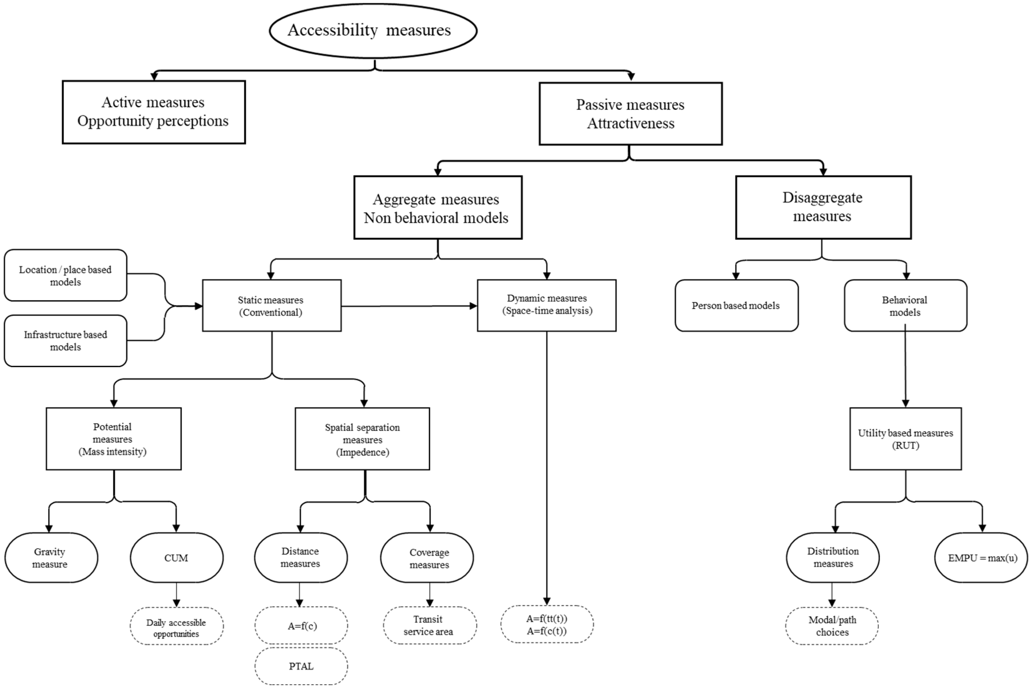
Figure 3.
Conceptual map of the accessibility measures reviewed from the literature. Description of active measures.
The proposed framework is made of three main levels. By the first, a distinction is made between active and passive accessibility, by which it is possible to separate two homonymous classes of accessibility measures. However, many of the methods allow a dual interpretation, so that it is possible to shift from one to the other typology of measure by adjusting the mathematical formulation, i.e., considering the origin that was the destination before. A second level concerns aggregate and disaggregate measures, leading to non-behavioral and behavioral models, respectively, since aggregate measures result from the integration of data collected from various sources in order to formulate relationships that connect objectively quantifiable spatial and temporal data, suggesting a detachment from behavioral evaluations. On the other hand, the disaggregated measures are not provided by the integration of experimental data and therefore do not intend to link objective or physical structures, so they are more inherent to behavioral evaluations (Figure 1). The third level means showing how to properly allocate the accessibility measures and mathematical models developed in the relevant literature. Conceptual maps of the accessibility measures reviewed from the literature are described in detail for passive measures (Figure 2) and for active measures (Figure 3).
In the following sections, we report an extensive literature review of the previous research focusing on passive (Section 3) and active accessibility measures (Section 4) as classified in the conceptual maps shown in Figure 1, Figure 2 and Figure 3.
To analyze the literature and identify accessibility measures and approaches, we used studies sourced from Scopus (https://www.scopus.com), Web of Science (https://www.webofscience.com), and ResearchGate (https://www.researchgate.net) from January to October 2024. Particularly, articles were filtered by keywords related to transportation, accessibility, sustainability, livability, GIS, spatial analysis, and walkability. In this review, only records labeled as “article” published in peer-reviewed journals in the English language were considered. This search yielded 249 results, and then after a thorough screening, we finally considered about 70 articles.
3. Passive Measures
A clarification of passive (and conversely also active) accessibility is given by Cascetta et al. [10], who define it as the total number of potential users available to move to a destination, as well as the ease recorded by a zone to be reached from all the potential users coming from all the other zones, i.e., the ability of a point of interest (e.g., wider neighborhoods, centroids or single facilities) to develop a peculiar attractiveness through the availability of services or infrastructures (e.g., transit stations or paths) around it [11]. Because of the strong reference to the geographic localization of the zone, seen as the destination zone of all the trips, this shape of accessibility can also be referred to as place accessibility [9]. This leads to the calculation methodologies of aggregated and integral data, which apply various conceptions of binding the involved opportunities with the assumed weights depending on locations or infrastructures features, and disaggregated measures, coming from the collection of hitched records used to model and predict human behavior (Figure 2).
3.1. Aggregate Measures—Non-Behavioral Models
Since Ingram [5] operates a distinction between integral and relative measures of accessibility, the first ones are defined as the degree of interconnection between a particular reference location and all the others in the study area. An integral measure is assumed to be derived by an analytic process that sums up opportunities capturing the weighting effects of impedance functions or parameters. This process of data aggregation typically results in conventional measures that take into consideration only one referring destination locality, ignoring the user behavior that, as an alternative, evaluates the utility of a trip among a group of potential travels, as well as perceptions or temporal limitations, even effective or alleged [12]. However, it is always possible to identify a finite pattern of opportunities to be taken into consideration and therefore a sort of intrinsic constraint.
Place-based models and infrastructure-based models are then the main conceptions related to the conventional measures, the originally built type of measures, also referred to as static measures because they define a value of accessibility that does not change during time or through space.
Place-based models are supposed to individuate locations that are external to the one considered the center of the analyzed system or the place whose accessibility value is required to be calculated.
Infrastructure-based models focus on the quality and performance of the transport network. They are generally recalled to group simple indicators, such as the congestion rate, total time lost and operating speed [13], which become simple to understand for both researchers and policymakers. However, they do not directly measure the attractiveness due to the presence of services and facilities, and this exclusion is not always assessed as a useful point of view. For example, most large city inner areas present high travel costs and time dispersion because of congestion; therefore, they should be marked by very poor accessibility, but they present higher levels of potential accessibility to jobs compared to suburbs [14]. Consequently, although these measures represent a well-defined panorama of contingent benefits for users, they cannot be used to predict future urban development or sprawl.
3.1.1. Static Measures: Potential Accessibility
A static measure of accessibility is provided by accounting for generalized indicators that are assumed to not vary temporally, considering either a single day or an extended time. When considering some objective features of places, facilities, or infrastructures, the available services may be seen to have a mass intensity able to generate a gravitational effect on users and land-use strategies [15]. Although, in many cases, it may be necessary to establish whether a research topic concerns a potential value, i.e., the theoretical maximum number of accesses, or an observed value, which presupposes investigations and studies of services and facilities [16], a static measure may nevertheless result in the application of a generalized model, as in the case of Hansen’s gravitational model [1], which leads to gravity measures, or a simple summation of opportunities or their users, as in the case of the cumulative opportunity method (CUM) [5], which is generally more suitable when considering smaller case studies.
Gravity measures are the mainstream expression of potential accessibility, considering the joint effect of a proper weight of each location and a weighting cost function, so that smaller or more distant opportunities provide a lower influence [8]. As the generic definition of accessibility is the ease with which a facility/opportunity can allow access to be used, the interpretation will be that of a passive measure, focusing on the centrality of the object that has to be reached. The main form is as follows:
where Ai is a measure of accessibility to a group of zones i from opportunities O in zones j, dij is the travel costs depending on the distance between i and j, and α is the cost sensitivity parameter. Since the travel cost factor must represent a distance decay function, the parameter α is negative and both the parameter and the function should be carefully chosen using the most recent empirical data on spatial travel behavior in the study area.
Gravity-like formulations are applied in several studies, admittedly with different weighting functions. One of the most used is the exponential function, which gives its name to a class of measures (exponential gravity-based measures) able to describe very well the land-use decay patterns. The measure has the following form, described by [1]:
where Oj will represent job locations or places to reach for a specific purpose inside the analyzed zone , receiving users from all the emitting zones , or the pure number of users incoming to .
It is worth remembering that, while it may be necessary to individuate a peculiar area in which a finite number of activities exist and for which it is possible to assess a more precise travel cost function, for many cases, it may be better to not impose any specific constraint around the analyzed centroid, as it is possible to individuate places or facilities external to the principal study area able to develop a shorter, but sometimes relevant, influence or attraction.
The cumulative opportunities method (CUM) [5] is an alternative solution for evaluating the attractiveness of a zone simply by counting the number of opportunities reached or reachable within a specified time threshold. The threshold might be seen as a boundary described by a function, which specifies the conditions for distinguishing between staying inside or outside a constraint.
where may represent the following:
- the number of inhabitants or job locations to reach into the considered zone ;
- the pure number of incoming travelers or incoming trips in the zone ;
- represents a selecting function to establish if the opportunity has to be accounted for or not, depending on a time constraint, being or the travel time range.
Due to its ease of applicability, it is a transparent and communicable measure [17]. Papa and Bertolini [18] explain that this type of measure does not acknowledge the gradual diminishing attractiveness of opportunities located farther away because of the lack of a weighting function. However, it can be applied at various levels with different time functions or constraints to understand how a zone becomes more or less attended by visitors coming for different purposes. Even if a threshold comes from specific considerations about the desired model (15 min, 20 min, 30 min), it is a common choice to take a 30 min frame, according to the approximate average time of work and study journeys [19].
3.1.2. Static Measures: Spatial Separation Measures
The physical distance between the origins of trips and the destinations may depend on contingent conditions that modify users’ path or mode choices, and therefore the trip length and time [20]. However, the level of separation between locations remains a very intuitive and simple indicator of the connectivity within a region. Curtis and Scheurer [21] explain that the spatial separation model can be categorized as an infrastructure-based measure, which does not take into account the behavioral aspects of travel choices. This implies that all opportunities are equally desirable, regardless of the time spent on traveling or the type of opportunity, creating a problem of the arbitrary selection of the isochrones (or isodistances) of interest and the lack of differentiation between opportunities adjacent to the origin and those just within the isochrones of interest. Thus, the measures are not very useful as input in social and economic evaluations of land-use and transport changes.
It is possible to divide two groups of spatial separation measures: those that account for geographical distances, travel times, monetary costs, or a combination of them [7] and those evaluating the range of an area covered by a service [22].
Distance measures rely on the quantification of the physical proximity between locations. The most simple and intuitive relation is [23]:
where dij is the shortest travel distance between centroids of zones or locations i and j. The strong limitation of this measure consists of the acknowledgement of the positions of opportunities since there might be a misunderstanding due to the accumulation of distances. If a place is reached by multiple users and trips, its cumulate accessibility increases, but being served by less users or trips that are further away produces the same cumulate value. Therefore, the interpretation of the relative value and the integral measure must be clarified depending on how large the model’s catchment area is.
A simple variation of the previous relation is [24]:
where Sij is a measure of the spatial separation, which may also be the travel time, and it may include weighting factors and exponents. For example, from Leake and Huzayyin [23]:
where tij is the minimum travel time between centroids i and j.
Measurements in this case are very easy, but they obviously completely neglect the quality of the paths and so the land-use distribution or the effective individual perception. They might be useful when locations are mainly straight-connected, as in simple neighborhoods or in models linking few facilities, ensuring that the accessibility calculation is inversely proportional to the distance and that it is corrected at most by factors linked to the travel mode or time dispersions due to access/egress to infrastructures. Moreover, the parameters are considered to not vary over time. They are easy to calculate for all the paths and user classes, such as in-vehicle time, access/egress times, waiting time or frequency of travel. Some studies prefer to evaluate distances in terms of the time used on the shortest path, especially when the trip is logically assumed to be the most efficient between a set of chances, e.g., reaching as quickly as possible job places or health services [25].
Bhat et al. [26] present a neat review of other formulations. It is worth remembering the following relation:
This is called the “Euclidean expression” [20]. Ek represents the mean expenditure per household on good k; and dij is the Euclidean distance to an activity in j in which the good k is available.
From Leake and Huzayyin [23], is the number of zones in the area, dij is the Euclidean distance between i and j centroids, and aij is the shortest travel distance between centroids.
From Ingram [5], is the average squared distance between all the points, and dij is the Euclidean distance between i and j centroids.
Again from Leake and Huzayyin [23], is the number of public transit routes serving zone i, is the length of route r (km) passing through zone i, and is the frequency of public transit (veh/h) operating over route r in zone i:
where N is the number of buses operating daily, T is the headway of the bus, and Tmax the longest operation time among all the buses serving the area i.
There are then accessibility indicators that use combinations of the distance measures. This is the case for the public transport accessibility level (PTAL) used to evaluate the number of transit access points within a maximum access time [27]. The model considers 8- or 12-minutes’ walk catchment areas, adding different waiting times depending on the reliability factors. The access times are then converted into frequencies, which are used to calculate the accessibility indexes (AI) for the single and compressive modes.
where the total access time (TAT) is determined by the summation of a waiting time (WT) and an average time (AWT), a function of the frequency of transit service. The final accessibility index accounts for the maximum and the relative equivalent doorstep frequencies (EDF).
Coverage measures evaluate the extent to which an area is covered by a service, or the degree of encompassing the needs of transport among a certain territory. These methods do not use any specific mathematical model, but they analyze networks with GIS software throughout the so-called service area tools (SAT) or time-based transit service area (TTSA). They incorporate and show on maps the total trips of transit services, so that it is possible to show all the locations that a passenger can reach within a proper time budget [22]. Ultimately, it is a combined application of the Hansen-type measures and the distance measures, thus providing an indicator of passive accessibility that takes into account how far a destination is touched and reached by passengers, following a few main steps: (i) defining an access time to transit stops for passengers and finding all the accessible terminals; (ii) finding all the accessible routes; (iii) calculating passengers’ in-vehicle time; (iv) identifying all the possible stops to disembark nearby the destination; (v) identifying portions of the travelable network for passengers with a remaining travel time budget; and (vi) producing a TTSA map showing the availability of opportunities.
3.1.3. Dynamic Measures
It has been said that the accessibility models that rely on the average values of access ease during the day are considered “static measures”, since the score for a specific location is assumed to be contingent and to not vary temporally. In some cases, this may not describe, at best, the level of access for different population groups and activity purposes, nor reflect real networks’ performances at different times of the day, made of peaks of traffic and free-flow patterns. For this reason, recent advances in spatial geography and transport engineering depict dynamic scenarios, recognizing that travel conditions can vary throughout a defined time span.
For example, Moya-Gómez and García-Palomares [28] aim to calculate the variation in accessibility every 15 min on a typical mid-week day. The intrinsic consideration is that, to evaluate accessibility from this point of view, it is necessary to define which static measures it is worthwhile to use and replicate. A static type of impedance may be defined by an adapted CUM:
where cij represents the impedance of traveling between two zones i and j, and aij is a binary variable that indicates whether an arc e is used or not, so that ce is the impedance of the arc e. The dynamic impedance, experienced for each instant t, is then described as:
where the parameters are referred to the instant m in which the arc is used and the instant t of beginning of the travel. The model wants to express that the shortest path possible is not always the same, so in typical GIS software multiple time-layers may be useful to show these dynamic phenomena.
The space–time analysis becomes one important concept in the formulation of dynamic measures, since when it is about to describe individuals’ multitude of roles, it is impossible to divide space coordinates from time coordinates. Hägerstrand [29] proposes a three-dimensional prism model, whose projection on the plane, called potential path area (PPA) or potential path space (PPS), represents and delimits the geographically constrained area containing the desired locations.
The prism can take on complex geometric shapes, but in its most simplified representation, it takes the form of two mirrored cones, for which the vertices fall on the starting point of the journeys and show the maximum time budget from that point. Kwan [12] explains that some of the main static indicators are involved into the potential path area theory [30], within which it is possible to define the number of opportunities, the length of networks, and the weighted number of opportunities, measuring gravity-based accessibility. The PPS design may be explicated as the “time availability” of an opportunity placed at location d. For Kwan [12], the total potential path for a transit service is:
where is the ending available time for the origin i, with the travel distance between origin and opportunity k and the velocity average value, and the starting time in the farest deadline j, diminished as the travel time from k to j. This formulation may be easily adapted, even to express the constraint if the destination k coincides with the center of the model, then overlapping the constraints from every origin to the same centroid destination, as a passive accessibility model.
Cascetta et al. [10] adapt the expression as follows:
where is a first potentially available event and is a final potentially available event for a same destination d, so that the potential path space will be defined by the interval between the instant (i.e., the starting time of the availability plus the necessary time to reach the destination d), and the instant (i.e., the final time of the last available opportunity minus the time to reach the destination). As the authors argue, since not every opportunity can have the same time constraint, even when placing a common restriction for including all of them, this analysis should only be applied at the scale of disaggregate models. As the PPA describes the availability of opportunities located at a certain distance, it is much more fitting as an active accessibility analysis than a passive one.
Kim and Kwan [31] show a GIS-based elaboration of the space–time prism, allowing them to calculate some accessibility measures with software and graphical help, where certain measures consider the pure geometric calculation of the PPA and the volume of the prism, ignoring the real uneven spatial distribution of opportunities or their time availability. Other measures account for the effective number of opportunities distributed inside the prism, either counting them as a cumulative measure or evaluating the volume of the prism shaping the time distribution with a realistic time function; others consider the uneven spatial distribution of opportunities, respecting the time availability of them singularly.
3.2. Disaggregate Measures
Common data collection methods are generally meant to combine the individual measurements to view the county statistics as a whole. Nevertheless, single data may be analyzed into specific hierarchies to obtain a closer look at relevant features. Therefore, talking about opportunities, spotted with or without geographical constraints, they can be singularly accounted for and divided into sub-categories. Categorizing them singularly or in groups, looking, for example, to users’ jobs or social classes, or to places’ street quality, and then not directly making them depend on a specific zone, distance or time, can reveal inequalities in their distribution [10].
Disaggregated measures may have a higher complexity of calculation, interpretation and communicability. However, they can express the availability of social and economic opportunities for individuals, even if their applications are often restricted to relatively small regions. Because of this analysis at the individual level, they are potentially useful for describing users’ trips through person-based measures, i.e., units based on their social characteristics [8].
The assumptions about user attributes and choice mechanisms lead to measures classified as behavioral. Behavioral models attempt to explain the decision-making processes of individuals, focusing on the net benefits obtained through voluntary choices of paths and travel modes. Therefore, they rely on capturing user preferences born from several evaluations of utility in making a trip. Utility measures are then the main core of behavioral models, expressing the total benefit associated with choosing an alternative, representing it in terms of probabilities.
Cascetta et al. [9] link behavioral models with disaggregate measures, defining accessibility through three levels of disaggregation:
The first equation identifies a relative measure depending on Pi(o), the population of a user’s class i at location o, and on the probability of finding the destination d in a set of choices (CS) for which an activity s is together available and perceived by a user as satisfactory. The second equation explicates the integral measure given by accounting for all the trips’ origins, so that a prime value of passive accessibility looks at the receiving destination d as collecting travelers from all the available sites and still categorizing them based on classes i. The third equation collects every user from every class, scope of travel, and origin, cumulating all the trips incoming to the same destination or centroid d.
3.2.1. Person-Based Measures
An accessibility measure based on people’s characteristics has a strong correlation with the individual freedom and willingness to perform an activity. For this reason, accessibility should be seen as the degree of deriving the maximum user benefit, eventually accounting for the socio-economic and physical restrictions that prevent travel. Person-based measures are considered very robust, since they can model large data populations, assessing their heterogeneity with precise constraints.
However, there are two main limitations. The first concerns the actual amount of data that case studies can take into account. As the population of data rises, it is possible to obtain more precise percentages from samples, but it is less easy to visualize the inevitable spreads linked to a large number of factors, and it becomes more necessary to pay attention to how spatial and personal variations in travel behavior can vary, depending on the analyzed portion of the population [19]. Hence, the second problem. While it is important to estimate individual preferences to travel, it is also necessary to ignore some characteristics (as age, gender, income, etc.) in order to achieve higher communicability, sometimes masking the inequity that exists within different socio-economic groups [32].
3.2.2. Behavioral Models—Utility-Based Measures
As has been said before, utility-based measures focus on the individual level, giving outcomes concerning short-term behavioral responses. It is useful to remember that long-term responses or patterns are actually foreseen with aggregate measures frameworks.
Utility-based measures can be divided into two types: one relying on the random utility theory (RUT) and another based on the doubly constrained entropy model [8]. The first uses the logsum, which is a summation of logarithmic values:
where Ai represents the maximum expected utility and Vk is the components, meaning various types of travel cost (distance, time, money, etc.). The unease of this approach is that varying Vk makes incompatible versions of Ai without the application of the pondered correction coefficients that compare and convert the parameters into economic values. Therefore, it is not often used to calculate accessibility. On the other hand, the benefit is that the formulation is simply derivable, so that allows calculations of user surplus.
The second approach depends on the spatial interaction model for trip distribution [33]:
in which Tij is the distribution of travel generated from each origin to each destination , constrained by the balancing factors Ai and Bj, depending on the inverse of a transport cost measure Cij, weighted by a sensitivity parameter .
Martínez and Araya [34] adapt the previous formulation, obtaining the following:
which truly represent the expected benefits per generated trips (Ai), attracted trips (Aj), and travel between two zones i and j (Aij). The advantage, in this case, consists of including competition effects in the measure.
4. Active Measures
Active accessibility measures evaluate the ease with which an activity can be reached by potential users, i.e., the ability of a user to reach relevant activities and opportunities consequent to the active choice of beginning a trip [35]. Therefore, accessibility measures evaluated from this perspective can reflect either the unconditioned necessity of reaching a place, independently of the behavior of the user, or consider the influence of the contour environment among users’ preferences. Methodologically, active accessibility accounted for without precise user behavior can be defined as an aggregate unit; accessibility accounted for when considering user behavior instead follows a disaggregate model (Figure 3).
4.1. Aggregate Measures—Non-Behavioral Models
Aggregate measures may be accounted for as descriptive measures, which belong to a class of non-behavioral models, since they reach for the functional relations between opportunities’ summation count and a consumptive parametrical indicator, not directly depending on customers’ preference considerations. They can be defined by simple category indexes or divided into generalized gravity-based measures or contour measures.
Some studies have seen a better analysis of these measures when applied to smaller scales, although active accessibility is defined by the active travel choices of both resident and non-resident workers in all kinds of neighborhoods, densely and non-densely inhabited [36,37].
4.1.1. Category Indexes
Category indexes represent the proportion of individuals within a particular group who are likely to engage in a specific activity, among a broader population of individuals in various roles. Since this indicates the likelihood or propensity of individuals within a specific category to undertake a particular trip among a set of activities, a category index can serve as a measure of the traffic flow in a trip generation model, belonging to the non-behavioral models.
They are generally used to make predictions about the traffic demand in mobility systems, allowing estimation of the origins–destinations matrixes based on the average number of travels made from users of category starting from an origin , in a precise time interval , for a scope [2]. The traffic flow can be then expressed as follows:
where is the overall number of users starting their trip from the same origin , and the factor expresses the proportion of them considered to be of the same category.
The models of category regression are a specification of non-behavioral emission models. They express the average value as a function, often linear, of variables relating to a same origin:
in which are generally average socio-economic variables, such as users’ income or number of owned cars, or they can include service-level attributes of specific areas.
4.1.2. Gravity-Based Measures
As said before, Hansen’s generalized gravity-based model [1] can measure the accessibility as a potential developed by a single or group of destinations among one or a set of origins, analogous to Newton’s gravitational effect:
- Oj represent opportunities located in external places , which may be job locations or places reached by users starting their trip from the emitting point “i”, or pure number of users going to .
- is the impedance factor that must always be calibrated, so as to make it inversely proportional to the travel distances or costs.
As active measures, gravity measures can either be the sum of the equivalent perceived opportunities reachable from a centroid or the effectively reached ones, always depending on an impedance factor. One of the strengths of this measurement is that unreachable destinations do not introduce anomalous values, so their opportunities are not taken into account. Reachable ones are those falling into a range, which can refer to some standard study cases, such as 15 min, 20 min or 30 min travel. However, when using a gravity measure, the definition of the traffic and road systems are more relevant than the effective zonal boundary for two reasons. First, there may be opportunities in the border regions that may strongly influence the accessibility values, so that it is preferable to never set an absolute geographic constraint [16]. Second, the traveled distances always depend on the transit mode of users, if by feet, car, rail or other, and even on the quality of the chosen paths, so that it may be more reasonable to think in terms of the employed times, unless it is possible to define purely univocal space–time relationships.
When analyzing a case of study, it is also important to precisely define the kind of interested targets, because different classes of opportunities present a peculiar distribution. For example, Shen [38] shows that job accessibility in inner cities neighborhoods, called central business districts (CBDs), may be signified by inequalities due to the uneven distribution of desired locations.
This means that there can exist a certain model ineffectiveness in communicating the availability of opportunities. In fact, while it is mainly considered the “supply side”, there are less focuses on the “demand side”, which has to be covered by accounting for both the total potential users that can make a trip, as people converging on a precise location, and users actively deciding to reach for it. This shape of accessibility indicator is expressed with gravity-deducted formulations as follows:
where:
- is the accessibility of people moving from location to destinations by travel mode ;
- are the opportunities located in destination places ;
- is the weighted travel demand of people moving to with travel modes ;
- is the number of people living in location and traveling by mode to seek opportunities;
- and are, respectively, the supply and demand functions of cost;
- and may eventually identify same travel modes, while and stand for the same origins.
An interesting case of study is depicted by Borghetti et al. [11] selecting walking areas in a 15-minute range (isochrone constraint), in which they detect different types of reachable amenities (hospitals, post offices, schools, supermarkets, pharmacies, libraries, theatres and cinemas, pubs, coffee bars, restaurants and EV charging points). A major number of available services around a transit rail station produce for it a higher level of attractiveness, weighted with an opportune exponential gravity-like function, so that the active measure can consist of the usage of those places around the point of interest and not of the point of interest itself.
A geographical definition of study areas is provided by Geertman and Ritsema Van Eck [39] and Gutiérrez et al. [40] formulating an average distance indicator based on an interpretation of the potential model. Since the transport systems’ efficiency is linked to the reaching time for key places and the gross product of job places, the average influence area will be defined by an iso-temporal buffer, increasing as the weights of the single spotted destinations grow. The so-called weighted average travel time (WATT) takes the form of:
where:
- is the proportional amount of population traveling from to ;
- is the measure of the travel distance between the origin and the referring centroid of a set of alternatives ;
- identifies the mass attraction, the total number of users, going to the area ;
- is the number of users specifically going to the activity .
- So that:
Cao et al. [41] show, in a case where the access to job locations is almost direct from the transit stop and the transportation services are evenly distributed on the territory, that the WATT indicator may be simplified to:
Obviously, the local accessibility does not depend on an average distance indicator, because of the lack of a distance decay factor. But when the total study area spreads to overly wide spaces, it becomes important to think about land development based on shorter buffers, proportional to activities’ localization [40].
4.1.3. Contour Measures
Geurs and van Wee [8] assume contour measures to be a derivation of distance measures when considering more than two possible destinations for the same origin and within a given travel time, distance or total cost. However, they do not suppose any intrinsic competition between the possibilities to reach one or the other destination; neither do they take individuals’ perceptions or preferences into account, meaning that all the opportunities intrinsically have the same chance to be picked.
The fixed constraints used to account for the reachable opportunities are mostly about:
- boundaries that can be reached within the same travel time, i.e., isochrones;
- boundaries that are equidistant from the origin point, i.e., isodistances;
- paths that allow the same or equivalent capacities for the same typologies of travelers.
Cao et al. [41] indicate this class of indicators to rely on the same application procedure of the CUM from Ingram [5], so that it is possible to define the daily accessible cities, the number of cities reachable from one origin within a specific travel time, or the daily accessible population, the amount of population that can be reached for a regional demand effect. The same aforementioned relationship, declined for active accessibility, will be:
with as the accessibility of a starting location , accounted for as the summation of the partial accessibility values depending on the single travel modes , those being the cumulation of reachable opportunities allocated in external zones, accounted for considering a constraint function.
Generally, the “daily accessibility” indicators consider a range of 3–4 h as the maximum admissible travel time to go and return within the day, to carry out a general activity or reach for economic activities in different cities [42]. Moreover, a distance constraint is generally less useful in urban environments due to the presence of road intersections and route disconnection points, so that the straight-line or Euclidean distances are rarely taken in consideration, unless for very small trips with linear space–time dependence.
When there is a mismatch between the spatial distribution of the population and the opportunities, or in general between the distribution of the demand and supply for a service, accessibility measures should consider competition effects. Several authors adopt different approaches to solve this issue [8]:
(1) Using a quotient of opportunities, dividing those defining the supply by the number of demand potential users [43], or considering the supplied opportunities and effectively reached ones, within a settled constraint [44].
(2) Using balancing dependent factors, with iterative procedures [45,46].
The first case is a solution also mentioned previously, when talking about applications of gravity-based measures. However, when considerations regarding the weight of individual opportunities are omitted, and when temporal or geographical constraints are deemed to be of greater relevance, a class of measures defined as the floating catchment area (FCA) arises.
As in the beginning they were used to evaluate job accessibility [47], they have been useful indicators in the GIS environment. The mainly used version of this measure is become the two-step floating catchment area (2SFCA) identified by the following formulations [44]:
where is the supply-to-demand ratio, calculated for each supply point j, dividing the number of supplied opportunities by the number of travelers , weighted by an impedance function . The impedance function is assessed to be a standardized Gaussian function, chosen because of its relatively slow decay rate near the origin, considering it to gradually vary as follows:
In a different study, cases have been proposed for modified constructions of the model, such as from Hu and Downs [48], who propose a supply-to-demand ratio defined as follows:
in which indicates the residential locations, is the number of workers and is a weighted Gaussian function.
However, there is always a limitation to consider when proposing a contour, consisting of which amenities to include in the analysis. In fact, travel distances may vary by person, their well-being, age, gender and culture, as well as by their trip purposes [49,50]. Threshold-based measures may introduce an “edge effect”, meaning that someone living outside a boundary, but very close to the edge, has not the same access as one living inside the constraint but also near the border. Therefore, using a single travel time for all the destinations may not suit a consistent evaluation of the accessibility. For this reason, the solutions with balancing factors generally referred to as double constrained models (DCMs) represent an accessibility measure ensuring that the magnitude of the flow originating from a zone must be equal to the number of reached activities [8].
The double constrained spatial interaction model (DCSI), proposed by Wilson [45] is expressed by the following mutually balanced formulations:
in which:
- is the number of encountered opportunities (job places) in destination locations ;
- is the balancing factor for the opportunities;
- is the number of demanding travels or travelers originating from locations ;
- is the balancing factor for the demand side;
- is the travel cost to reach destinations from , weighted by a sensitivity parameter .
4.2. Disaggregate Measures
It has been said previously that disaggregate measures exclude the integration of weighted opportunities over space or time. Since active measures focus on the individual decisions to engage in trips, disaggregate active measures need models and formulations that can help to quantify the impact of inter-dependent variables on trip-making choices. Generally, those variables are related to attributes mixed between the socio-economic characteristics of social groups, the quality level of a certain service and the quantitative measurements among alternatives.
When considering the active decision to begin a trip, it has to be clarified how a user perceives the attraction of activities located in a distant place and then which personal evaluations are performed about what is “worthy to be reached” [7]. Because of this, in many cases, it is necessary to refer to perception-based models. People may perceive different amounts of interest toward same destinations, regardless the objective or physical separation expressed through gravity measures, or they can assume a more or less realistic separation between origins and destinations, depending on their ability to objectively evaluate the urban space. The notation of perceived accessibility is linked to “the ease to live with the help of transport systems” [51], p. 258 although, according to Vitman-Schorr et al. [52], perceived accessibility is also influenced by non-transport factors such as social participation, safety feeling and effective security. It is often very useful to examine perceptions with structural equation models (SEMs), which may use regression models to reveal hidden mathematical patterns between several variables and perspectives [53,54,55].
Accessibility measures can also be obtained by behavioral models, where the will by which a choice occurs, considering it more convenient than others, is modeled through the user’s utility maximization, as described by RUT. Therefore, behavioral models generally lead to utility-based measures [10].
4.2.1. Perception-Based Models
Empirical knowledge of accessibility focuses on objective place-based measures [56], which allow us to take individual heterogeneity into account only to a limited extent [57]. Individual behavior is more highly sensitive to individual perceptions than objective accessibility measurements [58]. Curl [59] argues that using objective measures of spatial accessibility could obscure the inequities in accessibility that occur due to differences in perceptions of accessibility among individuals.
Current studies lean toward the idea that focusing on an individual user’s subjective perceptions is a more effective way to understand and evaluate accessibility. A user-centric approach pays attention to the specific traits of people, as they express different preferences depending on how they experience their own satisfaction in perceiving services’ features. Without capturing the lived experience of accessibility, it is not possible to assess the potential positive outcomes of accessibility, such as social inclusion and well-being [51].
Perceived accessibility is a subjective approach to assessing accessibility based on individuals’ preferences and attitudes as well as awareness of the level of ease of reaching and using transport systems, goods or services and activities [51]. Assessing the derived benefits of accessibility involves directly evaluating “how easy it is to live a satisfactory life with help of the transport system” using self-reported evaluations of accessibility [51], p. 258. Therefore, perceived accessibility is based “on peoples’ assessments of how the transport systems facilitate and enable them to perform the activities and live the lives they want, covering assessments of whole-trip experiences” [60], p. 2.
Pot et al. [61] define perceived accessibility as “the perceived potential to participate in spatially dispersed opportunities” (p. 2). It refers to an individual’s subjective assessment of the ease with which he or she can reach activity locations, and it differs from the so-called “objective” spatial elements that determine accessibility, being influenced by personal experiences, socio-economic factors and perceptions of the environment. As argued by Pot et al. [62], this involves assessing the level of participation in activities according to the perceived accessibility based on one’s needs, desires and abilities (accessibility-derived utility). Consequently, lower (higher) levels of participation may still correspond to high (low) self-reported levels of perceived accessibility.
Perceived analysis is based on survey or reported data [63]. A perceived approach is used in limited research studies [58,64,65,66]. Jamei et al. [67] propose a systematic review concerning the interpretations of perceived accessibility in the transportation field, the evaluation methods and the main influencing factors.
Using data from a self-administered survey in the Netherlands, Pot et al. [68] examine individual factors that explain the differences between the accessibility of daily activities calculated from spatial data and the perceived levels of accessibility in rural areas. An et al. [69] measure the perceived overall accessibility through a multicriteria subjective evaluation of individuals’ ability to reach regular destinations, services, and activities. Lukina et al. [70] analyze the difference between perceived (PA) and objective (OA) transport accessibility in the administrative districts of the Moscow metropolis (Russia). Ryan et al. [71] compare the perceived and measured accessibility between different age groups and travel modes in Perth (Australia).
The constructions that can explain the impact of attributes’ perceptions on choices are SEMs, generally more capable than regression models of solving problems of the correlation between latent variables due to the fact that simple regression models are just meant to find quick and relatable relationships that cannot incorporate sets of quality variables, hence underestimating the effect of a specific attribute in a built environment [54,72]. Moreover, van der Vlugt et al. [58] investigate the relations between travel attitudes, socio-demographic factors, objective walking accessibility, perceived walking accessibility and walking behavior by using the SEM approach. Chen et al. [73] analyze how individuals’ personal characteristics and neighborhood environment features influence the perceived accessibility of different types of activities by dockless bike-sharing in Beijing (China).
4.2.2. Behavioral Models—Utility-Based Measures
Mobility choices generally regard all the phases as composing a four-stage model: if starting a trip from an origin, what destination to pick, with what modality and on what path to travel. Evaluating every traveler separately, therefore accounting their behavior under a disaggregate point of view, accessibility is defined as a combined probability of reaching any of the destination starting from an origin [10]:
where:
- is the integral active accessibility for an individual of class (e.g., students or workers) that moves for a purpose activity ;
- is the total number of destinations;
- is the perceived choice set of locations accessible from an origin to individuals of the same class who begin a trip for the same activity scope ;
- is the probability to find a destination in a perceived choice set ;
- is the set of effectively available locations from the origin , spotted in a given spatio-temporal constraint;
- is the probability of finding a desired destination in the assessed constraint.
Generally, the adopted utility-based models belong to discrete choice models. The main formulation assessing how a user can make a choice is given by:
representing that the probability of picking an alternative inside a set of alternatives is due to the probability of expressing a utility higher than the utility of any other choice . Utility is composed of two contributions: the systematic value of a choice and the uncertainty value, so that:
The simplest discrete choice model is the multinomial logit model; a logit utility formulation evaluates the socio-economic conditions of users and the number of perceived services.
5. Discussion
The accessibility measures proposed in previous research (Section 3 and Section 4) are summarized in Table 1 under passive accessibility measures and in Table 2 as active accessibility measures. In each table, the pros and cons of applying the accessibility measures are highlighted.

Table 1.
Passive accessibility measures: pros and cons.
Table 2.
Active accessibility measures: pros and cons.
As shown in Table 1, passive accessibility measures are adequate for smaller case studies with a realistic representation of the spatial and temporal constraints. They ensure easy applications and simple calibrations of sensitivity parameters.
On the contrary, as reported in Table 2, active accessibility measures are needed prevalently for data disaggregation and then calibrations of the sensitivity parameters for specific cases. Their limited applicability is linked to the sample representativeness.
The main trends in terms of the accessibility measures are focused on users’ subjective perceptions of the travel experiences and satisfaction with service aspects, depending on their socio-economic characteristics, thus providing the concept of “perceived accessibility”.
6. Conclusions
Accessibility is a critical index representing the closeness of specific areas to various activities within a region. Evaluating how transport systems or environments facilitate interaction with services and relevant areas is important because opportunities are linked to the availability of activities within a region.
Accessibility has been evaluated using different approaches over time. Starting from the accessibility measures reported in the literature review, we derived an overview including measures based both on mathematics and physics and on social and economic studies. Consequently, we proposed a classification framework made up of three main levels. By the first, a distinction between active and passive accessibility is introduced. Active accessibility measures are defined as the ease with which users from the same origin can reach specific sets of opportunities distributed across the area. Passive accessibility refers to the potential number of users who can reach a destination, evaluating the ease with which a single destination can be accessed by users coming from different origins.
Secondly, we distinguished between behavioral and non-behavioral measures. Behavioral (non-aggregate) measures focus on individual user experiences and preferences, utilizing models that account for subjective evaluations and decision-making processes. Non-behavioral (aggregate) measures are discussed as descriptive indicators that aggregate data across various sources, providing a broader view of accessibility without delving into individual user behavior.
Measuring accessibility distances is crucial too, as the framework introduced in its third level considers how distances can be perceived differently by users, affecting their decision-making regarding travel. Distances are regarded as either a spatial or a temporal dimension, representing a metric that separates an origin from a destination. Evaluating this metric enables the understanding of the impedance a traveler may face in undertaking a specific journey. Impedance is then a core factor, representing the resistance or difficulty in reaching a destination.
Experimental evidence on accessibility mainly focuses on objective place-based measures, although individual behavior is more sensitive to individual perceptions than objective measures of accessibility. Future research directions are, therefore, oriented toward users’ subjective perceptions and perceived accessibility. People express different preferences according to their specific characteristics and the way they experience their satisfaction in perceiving the characteristics of services. In such a way, perceived accessibility is a subjective evaluation based on individuals’ preferences and attitudes as well as their awareness of the level of ease of reaching and using transport systems, goods or services and activities.
Studies on perceived accessibility have recently come to the forefront of the research [51,59,61,62,68], suggesting that traditional measures may not fully capture accessibility as experienced by individuals. These studies revealed a significant mismatch between the perceived and objective measures of accessibility. Therefore, further research is needed in this field of investigation.
Moreover, while the relationship between perceived accessibility and travel behavior has been well established, there is less knowledge regarding the relationship between travel behavior and accessibility as perceived by users. In a very recent study, Mehdizadeh and Kroesen [74] find that travel mode use has a larger impact on perceived mode-specific accessibility than the reverse. From a policy perspective, this implies that efforts to correct misperceptions about the accessibility of transport modes could still have a positive impact on individuals’ decisions to choose a public transport or active modes.
Author Contributions
Conceptualization, Gabriella Mazzulla; methodology, Gabriella Mazzulla and Carlo Giuseppe Pirrone; formal analysis, Gabriella Mazzulla and Carlo Giuseppe Pirrone; investigation, Gabriella Mazzulla and Carlo Giuseppe Pirrone; writing—original draft preparation, Gabriella Mazzulla and Carlo Giuseppe Pirrone; writing—review and editing, Gabriella Mazzulla and Carlo Giuseppe Pirrone; visualization, Carlo Giuseppe Pirrone; supervision, Gabriella Mazzulla. All authors have read and agreed to the published version of the manuscript.
Funding
This research was funded under the National Recovery and Resilience Plan (NRRP), Mission 4 Component 1 Investment 3.4—Call for tender No. 118 of 3.2.2023 of Italian Ministry of University and Research funded by the European Union—Next Generation EU, CUP H23C23001670005, grant n. 39-034-05-DOT1305040-10705.
Data Availability Statement
No new data were created.
Conflicts of Interest
The authors declare no conflicts of interest. The funders had no role in the design of the study; in the collection, analyses, or interpretation of data; in the writing of the manuscript; or in the decision to publish the results.
References
- Hansen, W.G. How Accessibility Shapes Land Use. J. Am. Inst. Plan. 1959, 25, 73–76. [Google Scholar] [CrossRef]
- Ben-Akiva, M.; Lerman, S.R. Disaggregate travel and mobility choice models and measures of accessibility. In Behavioural Travel Modelling; Hensher, D., Stopher, P., Eds.; Routledge: London, UK, 1979; pp. 654–679. [Google Scholar]
- Sharma, G.; Patil, G.R. Public transit accessibility approach to understand the equity for public healthcare services: A case study of Greater Mumbai. J. Transp. Geogr. 2021, 94, 103123. [Google Scholar] [CrossRef]
- Wegener, M.; Fuerst, F. Land-Use Transport Interaction: State of the Art. SSRN Electron. J. 2004, 1–119. [Google Scholar] [CrossRef]
- Ingram, D.R. The concept of accessibility: A search for an operational form. Reg. Stud. 1971, 5, 101–107. [Google Scholar] [CrossRef]
- Morris, J.M.; Dumble, P.L.; Wigan, M.R. Accessibility indicators for transport planning. Transp. Res. Part A 1979, 13, 91–109. [Google Scholar] [CrossRef]
- Baradaran, S.; Ramjerdi, F. Performance of Accessibility in Europe. J. Transp. Stat. 2001, 4, 31–48. [Google Scholar]
- Geurs, K.T.; van Wee, B. Accessibility evaluation of land-use and transport strategies: Review and research directions. J. Transp. Geogr. 2004, 12, 127–140. [Google Scholar] [CrossRef]
- Cascetta, E.; Cartenì, A.; Montanino, M. A New Measure of Accessibility based on Perceived Opportunities. Procedia-Soc. Behav. Sci. 2013, 87, 117–132. [Google Scholar] [CrossRef]
- Cascetta, E.; Cartenì, A.; Montanino, M. A behavioral model of accessibility based on the number of available opportunities. J. Transp. Geogr. 2016, 51, 45–58. [Google Scholar] [CrossRef]
- Borghetti, F.; Colombo, C.G.; Longo, M.; Mazzoncini, R.; Cesarini, L.; Contestabile, L.; Somaschini, C. 15-min station: A case study in north Italy city to evaluate the livability of an area. Sustainability 2021, 13, 10246. [Google Scholar] [CrossRef]
- Kwan, M.P. Space-time and integral measures of individual accessibility: A comparative analysis using a point-based framework. Geogr. Anal. 1998, 30, 191–216. [Google Scholar] [CrossRef]
- Butcher, L.; Codd, F.; Harker, R. Transport Policy in 2010: A Rough Guide; Research Paper 10/28; House of Common Library: London, UK, 2010. [Google Scholar]
- Linneker, B.J.; Spence, N.A. Accessibility Measures Compared in an Analysis of the Impact of the M25 London Orbital Motorway on Britain. Environ. Plan. A 1992, 4, 1137–1154. [Google Scholar] [CrossRef]
- Hanson, S.; Schwab, M. Accessibility and Intraurban Travel. Environ. Plan. A Econ. Space 1987, 19, 735–748. [Google Scholar] [CrossRef]
- Wang, J.; Du, F.; Huang, J.; Liu, Y. Access to hospitals: Potential vs. observed. Cities 2020, 100, 102671. [Google Scholar] [CrossRef]
- Bertolini, L.; le Clercq, F.; Kapoen, L. Sustainable accessibility: A conceptual framework to integrate transport and land use plan-making. Two test-applications in the Netherlands and a reflection on the way forward. Transp. Policy 2005, 12, 207–220. [Google Scholar] [CrossRef]
- Papa, E.; Bertolini, L. Accessibility and Transit-Oriented Development in European metropolitan areas. J. Transp. Geogr. 2015, 47, 70–83. [Google Scholar] [CrossRef]
- Páez, A.; Scott, D.M.; Morency, C. Measuring accessibility: Positive and normative implementations of various accessibility indicators. J. Transp. Geogr. 2012, 25, 141–153. [Google Scholar] [CrossRef]
- Guy, C.M. The Assessment of Access to Local Shopping Opportunities: A Comparison of Accessibility Measures. Environ. Plan. B 1983, 10, 219–238. [Google Scholar] [CrossRef]
- Curtis, C.; Scheurer, J. Planning for sustainable accessibility: Developing tools to aid discussion and decision-making. Prog. Plan. 2010, 74, 53–106. [Google Scholar] [CrossRef]
- Cheng, C.-L.; Agrawal, A.W. TTSAT: A New Approach to Mapping Transit Accessibility. J. Public Transp. 2010, 13, 55–72. [Google Scholar] [CrossRef]
- Leake, G.R.; Huzayyin, A. Accessibility measures and their suitability for use in trip generation models. Traffic Eng. Control 1979, 20, 566–572. [Google Scholar]
- Chang, H.S.; Liao, C.H. Exploring an integrated method for measuring the relative spatial equity in public facilities in the context of urban parks. Cities 2011, 28, 361–371. [Google Scholar] [CrossRef]
- Chen, X.; Jia, P. A Comparative Analysis of Accessibility Measures by the Two-Step Floating Catchment Area (2SFCA) Method. Int. J. Geogr. Inf. Sci. 2019, 33, 1739–1758. [Google Scholar] [CrossRef]
- Bhat, C.; Handy, S.; Kockelman, K.; Mahmassani, H.; Chen, Q.; Weston, L. Development of an Urban Accessibility Index: Formulations, Aggregation, and Application; Research Project 7-4938, Research Report Number 4938-4; Center for Transportation Research, University of Texas: Austin, TX, USA, 2000. [Google Scholar]
- Adhvaryu, B.; Chopde, A.; Dashora, L. Mapping public transport accessibility levels (PTAL) in India and its applications: A case study of Surat. Case Stud. Transp. Policy 2019, 7, 293–300. [Google Scholar] [CrossRef]
- Moya-Gómez, B.; García-Palomares, J.C. Working with the daily variation in infrastructure performance on territorial accessibility. The cases of Madrid and Barcelona. Eur. Transp. Res. Rev. 2015, 7, 20. [Google Scholar] [CrossRef]
- Hägerstrand, T. What about people in Regional Science? Pap. Reg. Sci. Assoc. 1970, 24, 6–21. [Google Scholar] [CrossRef]
- Miller, H.J. Modelling accessibility using space-time prism concepts within geographical information systems. Int. J. Geogr. Inf. Syst. 1991, 5, 287–301. [Google Scholar] [CrossRef]
- Kim, H.M.; Kwan, M.P. Space-time accessibility measures: A geocomputational algorithm with a focus on the feasible opportunity set and possible activity duration. J. Geogr. Syst. 2003, 5, 71–91. [Google Scholar] [CrossRef]
- Marwal, A.; Silva, E. Literature review of accessibility measures and models used in land use and transportation planning in last 5 years. J. Geogr. Sci. 2022, 32, 560–584. [Google Scholar] [CrossRef]
- Williams, C.W.L. Travel Demand Models, Duality Relations and User Benefit Analysis. J. Reg. Sci. 1976, 16, 147–166. [Google Scholar] [CrossRef]
- Martínez, F.; Araya, C. Transport and Land Use Benefits under Location Externalities Transport and Land Use Benefits under Location Externalities. Environ. Plan. A 2000, 32, 1611–1624. [Google Scholar] [CrossRef]
- Vale, D.S.; Saraiva, M.; Pereira, M. Active accessibility: A review of operational measures of walking and cycling accessibility. J. Transp. Land Use 2016, 9, 209–235. [Google Scholar] [CrossRef]
- Cervero, R.; Rood, T.; Appleyard, B. Job Accessibility as a Performance Indicator: An Analysis of Trends and Their Social Policy Implications in the San Francisco Bay Area. 1995. Available online: https://escholarship.org/uc/item/6mp941d9 (accessed on 15 July 2024).
- Cui, B.; Boisjoly, G.; El-Geneidy, A.; Levinson, D. Accessibility and the journey to work through the lens of equity. J. Transp. Geogr. 2019, 74, 269–277. [Google Scholar] [CrossRef]
- Shen, Q. Location characteristics of inner-city neighborhoods and employment accessibility of low-wage workers. Environ. Plan. B Plan. Des. 1998, 25, 345–365. [Google Scholar] [CrossRef]
- Geertman, S.; Ritsema Van Eck, J.R. GIS and models of accessibility potential: An application in planning. Int. J. Geogr. Inf. Syst. 1995, 9, 67–80. [Google Scholar] [CrossRef]
- Gutiérrez, J.; Gonzalez, R.; Gomez, G. The European high-speed train network: Predicted effects on accessibility patterns. J. Transp. Geogr. 1996, 4, 227–238. [Google Scholar] [CrossRef]
- Cao, J.; Liu, X.C.; Wang, Y.; Li, Q. Accessibility impacts of China’s high-speed rail network. J. Transp. Geogr. 2013, 28, 12–21. [Google Scholar] [CrossRef]
- Gutiérrez, J. Location, economic potential and daily accessibility: An analysis of the accessibility impact of the high-speed line Madrid-Barcelona-French border. J. Transp. Geogr. 2001, 9, 229–242. [Google Scholar] [CrossRef]
- van Wee, B.; Hagoort, M.; Annema, J.A. Accessibility measures with competition. J. Transp. Geogr. 2001, 9, 199–208. [Google Scholar] [CrossRef]
- Luo, W.; Wang, F. Measures of spatial accessibility to health care in a GIS environment: Synthesis and a case study in the Chicago region. Environ. Plan. B Plan. Des. 2003, 30, 865–884. [Google Scholar] [CrossRef] [PubMed]
- Wilson, A. Entropy in Urban and Regional Modelling; Pion: Billerica, MA, USA, 1970. [Google Scholar]
- Geurs, K.T.; Ritsema van Eck, R.J. Accessibility Measures—Review and Applications; National Institute of Public Health and the Environment: Bilthoven, The Netherlands, 2001. [Google Scholar]
- Wang, F. Modeling Commuting Patterns in Chicago in a GIS Environment: A Job Accessibility Perspective. Prof. Geogr. 2000, 52, 120–133. [Google Scholar] [CrossRef]
- Hu, Y.; Downs, J. Measuring and visualizing place-based space-time job accessibility. J. Transp. Geogr. 2019, 74, 278–288. [Google Scholar] [CrossRef]
- Schaap, N.; Harms, L.; Kansen, M. Cycling and Walking: The Grease in Our Mobility Chain; KiM Netherlands Institute for Transport Policy Analysis: Apeldoorn, The Netherlands, 2016. [Google Scholar]
- Logan, T.M.; Hobbs, M.H.; Conrow, L.C.; Reid, N.L.; Young, R.A.; Anderson, M.J. The x-minute city: Measuring the 10, 15, 20-minute city and an evaluation of its use for sustainable urban design. Cities 2022, 131, 103924. [Google Scholar] [CrossRef]
- Lättman, K.; Olsson, L.E.; Friman, M. Development and test of the perceived accessibility scale (PAC) in public transport. J. Transp. Geogr. 2016, 54, 257–263. [Google Scholar] [CrossRef]
- Vitman-Schorr, A.; Ayalon, L.; Khalaila, R. Perceived Accessibility to Services and Sites Among Israeli Older Adults. J. Appl. Gerontol. 2019, 38, 112–136. [Google Scholar] [CrossRef] [PubMed]
- van Kesteren, E.J. Structural Equations with Latent Variables; John Wiley & Sons: Hoboken, NJ, USA, 1992. [Google Scholar]
- Cao, X.J.; Næss, P.; Wolday, F. Examining the effects of the built environment on auto ownership in two Norwegian urban regions. Transp. Res. Part D Transp. Environ. 2019, 67, 464–474. [Google Scholar] [CrossRef]
- Liu, Y.; Ding, X.; Ji, Y. Enhancing Walking Accessibility in Urban Transportation: A Comprehensive Analysis of Influencing Factors and Mechanisms. Information 2023, 14, 595. [Google Scholar] [CrossRef]
- Lättman, K.; Olsson, L.E.; Friman, M. A new approach to accessibility—Examining perceived accessibility in contrast to objectively measured accessibility in daily travel. Res. Transp. Econ. 2018, 69, 501–511. [Google Scholar] [CrossRef]
- Curl, A.; Nelson, J.D.; Anable, J. Same question, different answer: A comparison of GIS-based journey time accessibility with self-reported measures from the National Travel Survey in England. Comput. Environ. Urban Syst. 2015, 49, 86–97. [Google Scholar] [CrossRef]
- van der Vlugt, A.L.; Curl, A.; Scheiner, J. The influence of travel attitudes on perceived walking accessibility and walking behaviour. Travel Behav. Soc. 2022, 27, 47–56. [Google Scholar] [CrossRef]
- Curl, A. The importance of understanding perceptions of accessibility when addressing transport equity: A case study in Greater Nottingham, UK. J. Transp. Land Use 2018, 11, 1147–1162. [Google Scholar] [CrossRef]
- Chau, H.W.; Gaisie, E.; Jamei, E.; Chan, M.; Lättman, K. Perceived Accessibility: Impact of Social Factors and Travel Modes in Melbourne’s West. Appl. Sci. 2024, 14, 6399. [Google Scholar] [CrossRef]
- Pot, F.J.; van Wee, B.; Tillema, T. Perceived accessibility: What it is and why it differs from calculated accessibility measures based on spatial data. J. Transp. Geogr. 2021, 94, 103090. [Google Scholar] [CrossRef]
- Pot, F.J.; Heinen, E.; Tillema, T. Sufficient access? Activity participation, perceived accessibility and transport-related social exclusion across spatial contexts. Transportation 2024. [Google Scholar] [CrossRef]
- Merlin, L.A.; Jehle, U. Global Interest in Walking Accessibility: A Scoping Review. Transp. Rev. 2023, 43, 1021–1054. [Google Scholar] [CrossRef]
- Boakye-Dankwa, E.; Barnett, A.; Pachana, N.A.; Turrell, G.; Cerin, E. Associations Between Latent Classes of Perceived Neighborhood Destination Accessibility and Walking Behaviors in Older Adults of a Low-Density and a High-Density City. J. Aging Phys. Act. 2019, 27, 553–564. [Google Scholar] [CrossRef] [PubMed]
- Erath, A. Modelling for Walkability: Understanding pedestrians’ preferences in Singapore. In Environmental Science, Engineering, Geography; IVT, ETH Zurich: Zurich, Switzerland, 2015. [Google Scholar] [CrossRef]
- Iacono, M.; Krizek, K.; El-Geneidy, A. Access to Destinations: How Close Is Close Enough? Estimating Accurate Distance Decay Functions for Multiple Modes and Different Purposes. In Environmental Science, Engineering, Geography; Minnesota Department of Transportation: Saint Paul, MN, USA, 2008. [Google Scholar]
- Jamei, E.; Chan, M.; Chau, H.W.; Gaisie, E.; Lättman, K. Perceived Accessibility and Key Influencing Factors in Transportation. Sustainability 2022, 14, 10806. [Google Scholar] [CrossRef]
- Pot, F.J.; Koster, S.; Tillema, T. Perceived accessibility in Dutch rural areas: Bridging the gap with accessibility based on spatial data. Transp. Policy 2023, 138, 170–184. [Google Scholar] [CrossRef]
- An, Z.; Mullen, C.; Guan, X.; Ettema, D.; Heinen, E. Shared micromobility, perceived accessibility, and social capital. Transportation 2024. [Google Scholar] [CrossRef]
- Lukina, A.V.; Sidorchuk, R.R.; Mkhitaryan, S.V.; Stukalova, A.A.; Skorobogatykh, I.I. Study of Perceived Accessibility in Daily Travel within the Metropolis. Emerg. Sci. J. 2021, 5, 868–883. [Google Scholar] [CrossRef]
- Ryan, M.; Lin, T.; Xia, J.; Robinson, T. Comparison of perceived and measured accessibility between different age groups and travel modes at Greenwood Station, Perth, Australia. Eur. J. Transp. Infrastruct. Res. 2016, 16, 406–423. [Google Scholar] [CrossRef]
- Zhang, W.; Zhao, Y.; Cao, X.J.; Lu, D.; Chai, Y. Nonlinear effect of accessibility on car ownership in Beijing: Pedestrian-scale neighborhood planning. Transp. Res. Part D Transp. Environ. 2020, 86, 102445. [Google Scholar] [CrossRef]
- Chen, Z.; van Lierop, D.; Ettema, D. Perceived accessibility: How access to dockless bike-sharing impacts activity participation. Travel Behav. Soc. 2022, 27, 128–138. [Google Scholar] [CrossRef]
- Mehdizadeh, M.; Kroesen, M. Does perceived accessibility affect travel behavior or vice versa? Alternative theories testing bidirectional effects and (in)consistency over time. Transp. Res. Part A 2025, 191, 104318. [Google Scholar] [CrossRef]

Disclaimer/Publisher’s Note: The statements, opinions and data contained in all publications are solely those of the individual author(s) and contributor(s) and not of MDPI and/or the editor(s). MDPI and/or the editor(s) disclaim responsibility for any injury to people or property resulting from any ideas, methods, instructions or products referred to in the content. |
© 2024 by the authors. Published by MDPI on behalf of the International Society for Photogrammetry and Remote Sensing. Licensee MDPI, Basel, Switzerland. This article is an open access article distributed under the terms and conditions of the Creative Commons Attribution (CC BY) license (https://creativecommons.org/licenses/by/4.0/).