Multi-Scale Effects of Supply–Demand Changes in Water-Related Ecosystem Services Across Different Landscapes in River Basin

Abstract

To promote sustainable hierarchical management, it is essential to understand the complex relationships within and underlying causes of supply–demand changes in water-related ecosystem services (WESs) across different spatial scales and landscape patterns. Consequently, the Optimal Parameters-based Geographical Detector (OPGD) and Multi-Scale Geographically Weighted Regression (MGWR) are used to analyze the factors influencing changes in WESs supply–demand. The findings indicate that (1) at the macroscale, population size, and economic activity are the main driving factors, while at the microscale, precipitation becomes the primary factor influencing fluctuations in WESs supply–demand. (2) Furthermore, over time, the influence of social factors becomes increasingly significant. (3) The explanatory power of a single factor typically increases as it interacts with other factors. (4) Abundant precipitation helps in the generation and maintenance of WESs, but intense human activities may have negative impacts on them. Therefore, we have made significant progress in identifying and analyzing the natural and human-induced driving forces affecting changes in WESs by deeply integrating long-term multi-source remote sensing data with the OPGD and MGWR models.

1. Introduction

Ecosystem services (ESs) are a range of benefits that ecosystems provide to humans, both directly and indirectly. They play a crucial role in promoting sustainable development by supplying essential resources and services, facilitating the coordinated development of the economy, society, and the environment, and ultimately supporting the achievement of global sustainable development goals [1]. These benefits emphasize the inseparable interconnectedness of humans and ecosystems, serving as fundamental links between human society and the natural world. These connections underscore the importance of protecting and sustaining these vital services for the continued survival of life on Earth [2]. However, human activities significantly impact ecosystem resilience and resistance due to the rapid acceleration of urbanization and population growth, which may lead to a decline in the capacity of ecosystems to provide essential services [3]. On the other hand, severe weather events—such as rising temperatures, uneven precipitation distribution, and heavy downpours—have also seriously harmed and disrupted ecosystems’ ability to adapt and function [4]. Growing ecological challenges have emerged from this supply–demand mismatch, which has become a significant contributor to environmental problems in many regions [5,6,7]. As vital components of ESs, water-related ecosystem services (WESs) play a significant role in enhancing both the natural environment and human well-being [8,9,10]. The supply capacity of WESs has inevitably been diminished due to significant changes in land use and cover (LULC) on the Earth’s surface, resulting from human activities and economic growth [11]. This leads to decreased soil carbon storage [12], unstable biodiversity [13], inadequate water purification [14], and increased soil erosion [15]. Consequently, the study of the supply–demand relationship of WESs has gained significant attention in academic circles due to its crucial role in formulating more rational and scientific intervention measures or policies, implementing effective ecosystem conservation plans, and advancing ecological compensation schemes.

The supply capacity of WESs has inevitably been weakened due to substantial changes in LULC on the Earth’s surface caused by human activities and economic growth [16]. This leads to decreased soil carbon storage [17], unstable biodiversity [18], inadequate water purification (WP) [19], and increased soil erosion [20]. Consequently, research into the supply-and-demand relationship of WESs has garnered significant attention in academic circles due to its critical role in formulating more rational and scientifically sound intervention measures or policies, implementing effective ecosystem conservation plans, and advancing ecological compensation schemes [21]. To identify LULC policy options that align with regional ESs supply–demand, Jain et al. [22] developed a multi-method retrospective model that integrates normative visions with exploratory LULC and ESs modeling. In the context of economic growth and urbanization, Wang et al. [23] analyzed the spatio-temporal patterns and shifts in the supply–demand of ESs and discussed their interactions. Guan et al. [24] identified the features of spatial coupling variations in the supply–demand of ESs between 1985 and 2015. Xu et al. [25], using a typical arid region as a case study, integrated participatory surveys to assess the magnitude of ESs demand and examined the supply–demand linkages of various ESs from the perspectives of multiple stakeholders. However, the socio-economic characteristics of ecosystem supply–demand relationships can only be considered at federal, provincial, or county levels through model development. This approach cannot quantify the geographical linkages between ecosystem supply–demand on natural attributes. Additionally, field surveys are limited in their ability to capture ecosystem supply–demand linkages in small or specific areas, making them insufficient for assessing spatial linkages over larger regions.

Most existing research presents only static data on the supply–demand linkages of ESs based on geographical patterns, and there remains room for improvement in the accuracy of these data. The dynamic nature of ESs can be reflected in variations in their supply–demand. Including the spatial features of these changes may provide a more comprehensive understanding of the relationship between energy supply–demand. Additionally, there are regional and spatial connections between the supply–demand of ESs [26]. The correlation levels between changes in supply–demand may fluctuate due to the geographical instability of natural environments and socio-economic conditions in different areas. In some cases, employing global spatial analysis techniques can result in a vague representation of the data. Research into the characteristics of shifts in the supply–demand of WESs still has notable information gaps. Therefore, zoning based on the spatial patterns of variations in WESs supply–demand is a valuable approach. This method allows spatial units within each region to visualize changes in WESs supply–demand, helping to accurately describe the correlation between these changes.

Based on actual demands, researchers have assessed WESs across various geographical scales to obtain clear information for their management [27,28]. However, the issue of scale is complex because supply–demand scales are not always consistent [29,30,31]. Generally, a variety of ecological scales—including vegetation, landscape, and ecosystem levels—are involved in the provision of WESs [32,33]. The demand for WESs is driven by various social and organizational scales, such as individuals, households, administrative units, and global trends [34,35,36]. A scale mismatch occurs when the scale of social organizations that utilize or manage the ecological environment does not align with the scale of natural environmental changes. This can lead to conflicts, inefficiencies, or oversights in policy decision-making [37]. In other words, depending on the assessment’s observational scale, the interactions and spatial patterns of the mismatch between the supply–demand of WESs may vary [38]. While many studies have focused on the supply–demand of WESs, much of this research is limited to a single geographical scale, such as cities, watersheds, or arid regions [39,40]. This focus overlooks the spatial dependency in the interactions between the supply–demand of WESs over a range of periods and scales [41]. The matching types observed at a single scale can be misleading for understanding the supply–demand connections of ESs and may not serve as valid references for other scales, a fact acknowledged by only a few researchers [42,43]. For instance, Baró et al. [44] found that the supply–demand of ESs in Berlin, Germany, were mismatched at the neighborhood level but aligned at the municipal level. Liu et al. [45] noted an increasing discrepancy between the supply and the demand for energy-related products in the Yangtze River Economic Belt, with some regions experiencing a surplus rather than a deficit. In summary, conducting ecological environment evaluations at various administrative levels—including county, township, province, and city—facilitates the implementation of policies at the appropriate scale. At the microscale, grid evaluation units can help disentangle administrative and spatial disparities in ecological restoration and conservation. However, capturing the hierarchical signals of regional ecosystem management remains challenging, as no studies have yet assessed changes in the supply–demand of WESs across different administrative and grid sizes.

Different scales influence the supply–demand patterns, matching status, and driving forces of WESs. These forces also reflect various scale properties and spatial features [46]. Numerous studies have employed diverse techniques to evaluate the spatiotemporal changes in the supply–demand characteristics of ESs [47]. Research methods such as Geographical Detector (Geo-Detector), Partial Least Squares Structural Equation Modeling (PLS-SEM), Ordinary Least Squares (OLS), Random Forest Regression (RFR), and Geographically Weighted Regression (GWR) are among those used to analyze driving processes [48,49,50]. Among these approaches, the Geo-Detector method is particularly effective at accurately identifying and interpreting the driving factors influencing the system of interest [51]. This model can reveal the interactions between driving variables and Ess, as well as the inherent processes linking them, without requiring a linear assumption. However, the geographic statistical units of ESs and the methods used for determining driving variables significantly impact the results, depending on the scale and zoning method applied in the research. Previous studies often relied on empirical scaling of geographical data, using the Jenks Natural Breaks approach to divide explanatory variables—a method that is influenced by human subjectivity and lacks precision [52]. The spatial variance partitioning technique (Optimal Parameters-based Geographical Detector, OPGD) calculates geographical variation across and within sub-regions, allowing for the division of explanatory variables into sub-regions and assessing the strength of the driving factors [53]. This approach is particularly useful for examining the spatiotemporal features of and potential driving forces behind changes in the supply–demand of WESs, as it effectively addresses the Modifiable Areal Unit Problem (MAUP) and the impact of driving variable division. While multivariate analyses can provide insights into the effects of various driving factors on changes in ecosystem supply–demand, the results of ordinal analyses typically reveal driving mechanisms only from a global statistical perspective, lacking spatial explicitness in the ecological processes involved.

Thus, it has become increasingly important to examine how to monitor these occurrences locally and to incorporate more precise geographical information. For instance, OLS is often used to model the spatial correlations between multiple independent variables and the dependent variable under diverse geographic conditions. However, this modeling approach fails to account for spatial heterogeneity, particularly in ecological systems that inherently exhibit spatial non-stationarity [54]. GWR addresses this limitation by quantifying various spatial correlations at multiple locations from a local perspective using its regression parameters, effectively filling the gap left by global regression methods [55]. By allowing variable coefficients to fluctuate at different geographical locations, the GWR model expands upon traditional regression frameworks and successfully addresses spatial heterogeneity [56,57]. A constant spatial scale proves ineffective, as the spatial processes underlying geographical phenomena are inherently diverse. Moreover, the fixed bandwidth used by the GWR approach for different variables can result in biased parameter estimates [58]. The most recent iteration of GWR, Multiscale Geographically Weighted Regression (MGWR), offers advantages for characterizing the geographically diverse relationships between response variables and explanatory factors. It takes into account the varying spatial scales of distinct surface characteristics. To better understand the features of changes in WESs supply–demand at both local and global scales, it is crucial to investigate the combined approach of OPGD and MGWR and to conduct a thorough analysis of the landscape changes brought about by these potential causes. While previous research has empirically analyzed and explored the supply–demand for ESs with varying degrees of success across different areas, theories, and techniques, there has been limited systematic research on the processes, scale impacts, and causes of dynamic variations in WESs supply–demand. This gap complicates the ability of policymakers to develop effective hierarchical management strategies that operate at multiple levels and consider socio-ecological feedback when allocating resources.

The Yangtze River Basin (YRB) is a major environmental asset and a biodiversity gene bank for China, characterized by rapid urbanization and significant ecological support capacities [59]. However, recent decades have seen the emergence of environmental degradation issues in the YRB due to the swift increase in urbanization [60]. This study quantitatively identifies the spatial structure of WESs supply–demand in the YRB from 2000 to 2020 at the basin level. When zoning the area ecologically, the geographical features of the variations in WESs supply–demand are taken into account. The driving forces behind these variations in different environments are investigated using OPGD and MGWR. Understanding the cross-scale dynamics of ecosystem supply–demand changes is essential for guiding the development of sustainable ecosystems and implementing effective solutions. Consequently, the YRB serves as a case study in this research, which aims to achieve the following goals: (1) to evaluate the spatial mismatch pattern of changes in WESs supply–demand at three grid scales and the county level; (2) to analyze the scale effects of driving factors on the spatial changes in WESs supply–demand through comparisons across various regions; and (3) to ascertain the focused, effective, and localized impact of different decision-making levels on stratified WESs management.

2. Materials and Methods

2.1. Study Area

The YRB is located between 90°33′ E–122°25′ E and 24°30′ N–35°45′ N in central China (Figure 1). Covering an area of approximately 1.8 million km², it is the largest river basin in China and the third largest in the world, accounting for roughly 18.8% of the country’s total land area [61]. The YRB encompasses three distinct climatic zones: the central subtropical monsoon, the southwest tropical monsoon, and the cold zone of the Qinghai–Tibet Plateau. Alpine meadows and natural grasslands dominate the upstream regions, while the midstream areas are characterized by various types of woodland vegetation. The downstream regions are primarily agricultural. This diversity in landscapes supports a wide range of plant species [62]. The YRB experiences erratic temporal and geographical distributions of precipitation, with an average annual rainfall ranging from 300 to 2400 mm. Rainfall patterns, which are primarily concentrated in May, June, and September, are influenced by the terrain and water vapor transport pathways. The typical temperature ranges from 4 to 24 °C [63]. The multi-year average temperature is higher in the southeast than in the northwest, and there is a decreasing trend in precipitation from the southeast to the northwest. The region’s topography, which alternates between mountainous, hilly, and plain terrains, contributes significantly to the geomorphic variations within the YRB. As a result, numerous geomorphic types have emerged, including the Sichuan Basin, the Dongting Lake Plain, and the Yangtze River Delta. The YRB has a substantial impact on China’s economy, culture, and natural resources, making it one of the nation’s most significant, diverse, and expansive river basins. It serves as a crucial site for grain production, acts as an ecological green barrier, and is a vital strategic water source for China. However, in recent years, the basin has increasingly experienced drought disasters. The rapid urbanization of the region has diminished ecosystems’ ability to provide essential functions, exacerbating the conflict between societal growth and environmental preservation.

2.2. Data Description

Table 1. Primary sources of information and data for this investigation.

Data Type	Period	Spatial Resolution	Data Sources
LULC data	2000, 2010, 2020	30 m	Resource and Environment Science and Data Centre (RESDC, http://www.resdc.cn/, DOI: 10.12078/2018070201), accessed on 3 April 2024
Digital elevation model (DEM)	—	30 m	Geospatial data cloud platform (http://www.gscloud.cn/), accessed on 4 April 2024
Slope	—	30 m	Using DEM data, the required terrain information was extracted through ArcGIS 10.6.1 software. Accessed on 3 March 2024
Soil data	—	1 km	RESDC
Meteorological data (temperature, precipitation, evapotranspiration)	2000, 2010, 2020	1 km	China Daily Surface Climate dataset (V3.0) (http://data.cma.cn), accessed on 3 April 2024
Normalized difference vegetation index (NDVI)	2000, 2010, 2020	250 m	https://modis.gsfc.nasa.gov/data/, accessed on 21 March 2024
Nighttime-light dataset	2000, 2010, 2020	1 km	https://data.tpdc.ac.cn/, accessed on 19 March 2024
Population	2000, 2010, 2020	1 km	Statistical Yearbook in China, accessed on 12 March 2024
Gross domestic product (GDP)	2000, 2010, 2020	1 km	Statistical Yearbook in China, accessed on 12 March 2024
Water consumption	2000, 2010, 2020	—	Water resources bulletin, accessed on 12 March 2024

presents a multi-source data collection used for a geographic quantitative study of WESs supply–demand. This dataset includes spatial and statistical information for the years 2000, 2010, and 2020. The spatial data encompass various types, such as soil characteristics, LULC, digital elevation model (DEM), normalized difference vegetation index (NDVI), nighttime light, and meteorological data. The statistical data include parameters like nitrogen content, water usage, population, and gross domestic product (GDP). We projected the geographic data using the Krasovsky_1940_Albers coordinate system, resampling it to a pixel resolution of 500 m × 500 m with ArcGIS 10.6.1 software.

2.3. Framework of This Study

This study investigates the supply–demand of WESs in the YRB from 2000 to 2020, focusing on their evolutionary characteristics, as well as their temporal and geographical trends. To better understand the dynamic relationships between fluctuations in WESs supply–demand across various landscape patterns and the characteristics of the influencing variables, this research considers both natural ecosystems and socio-economic systems. Figure 2 (see Section 2.4) presents a framework established based on the socio-ecological conditions in China and the theoretical framework of ecosystems. The methodology consists of five steps aimed at exploring the causes of similarities or discrepancies in WESs supply–demand across different scales and extended periods. (1) Selection of Key WESs: Important WESs, such as nitrogen export, soil conservation, and water yield (WY), were identified. Appropriate geographic scales for analysis were established, including county-level scale and grid data at 1 km, 3 km, and 12 km (see Section 2.4). (2) Spatial Quantification: The spatial quantification of water output, soil conservation (SC), and nitrogen export was conducted at a 500 m scale for the years 2000, 2010, and 2020 using ecological models and nighttime light pixel proportion techniques. These quantitative results were then aggregated to larger scales (county-level, 1 km, 3 km, and 12 km grids), with supply–demand values for WESs generated using an equal weight overlay approach (see Section 2.5 and Section 2.6 for details). (3) Geographical Distribution Analysis: From a multi-scale perspective, we determined geographical distribution maps of hot and cold spots for variations in WESs supply–demand using the bivariate Moran’s I index. We analyzed the geographical patterns of nine categories of WESs supply–demand imbalances and their homogeneous zones by comparing the spatiotemporal changes in WESs supply–demand between 2000 and 2010 and from 2010 to 2020 (see Section 2.7 for details). (4) Investigation of Influencing Processes: We examined the underlying processes influencing variations in WESs supply–demand at four different scales using the OPGD method. To further explore the regional variability of these driving factors, we also employed the MGWR approach. (5) Development of a Decision-Making Framework: based on our findings, we developed a comprehensive framework for ecological environment management strategies tailored to various river basin, county, provincial, and finer management scales.

2.4. Selection of the Critical WESs and Scales

(1) Selection of WESs: The provision of clean freshwater from upstream headwaters is one of the primary environmental services that watersheds offer to human communities [64]. However, LULC changes, along with climate change, can significantly affect a basin’s ability to manage the hydrological cycle, as well as regulate the quantity and quality of water. For instance, deforestation, urbanization, and agricultural expansion may lead to increased water consumption, reduced infiltration, and deteriorating water quality. Moreover, shifts in climate patterns could cause more frequent and intense droughts and floods. These changes could profoundly impact the ESs that watersheds provide, particularly the source of clean water [65]. One of the most vital ESs offered by watersheds is water filtration. This service involves the use of natural processes to remove pollutants and improve water quality, making it suitable for various uses, including human consumption. WP services are critical to maintaining the health of aquatic ecosystems and supporting human well-being [66]. Given the significant role of WESs in the YRB, this study focuses on three specific WESs: WY, SC, and WP.

(2) Examination of Scale Selection: One of the key decision-making dimensions for ecological preservation and spatial planning is the county level [67]. At this scale, it is crucial to balance urban development with the protection of WESs to reduce the conflict between human activities and the natural environment, fostering their harmonious coexistence. Striving for this balance moves us closer to the goal of sustainable, green development by establishing a new kind of human–water relationship [68]. In May 2022, the General Offices of the State Council and the Communist Party of China Central Committee issued the “Opinions on Promoting Urbanization Construction with Counties as Important Carriers”. This document clearly outlines that counties will be the primary focus of future urbanization efforts in China, aiming to raise the overall development level of counties as key implementation units. At the same time, the 1 km grid, a fundamental ecological unit, has been widely used to evaluate the supply–demand of WESs at various scales, including cities, provinces, and urban agglomerations [69]. In China, ecosystem conservation and restoration efforts are typically carried out at the national, provincial, and county levels [70,71,72], with limited attention paid to more localized management at the township level. Additionally, management actions often do not align with the actual scope of ecological changes [73]. At the same time, the research scale of WESs in suburban basins and areas near cities (demand–supply) in different regions is relatively small, and the data require refinement. Currently, the data cannot be obtained and will not be considered for the time being [74]. Therefore, policymakers should consider the true extent of WESs, rather than being constrained by administrative boundaries, when designing management strategies [75,76]. To obtain data at different grid scales, we created 3 km, 5 km, 10 km, 12 km, and 15 km grids using the ‘Create Fishnet’ tool [77]. Preliminary analyses revealed differences in the distribution of supply–demand across scales. For example, the average township size in the YRB is approximately 8.6 km² for the 3 km grid and 146 km² for the 12 km grid. Furthermore, the 3 km grid is often used as the basic ecological unit for national ecological evaluations [78,79]. In summary, the final scale selection for this study included county-level grids, as well as 1 km, 3 km, and 12 km grids, to better align the evaluation scale with management needs [80,81].

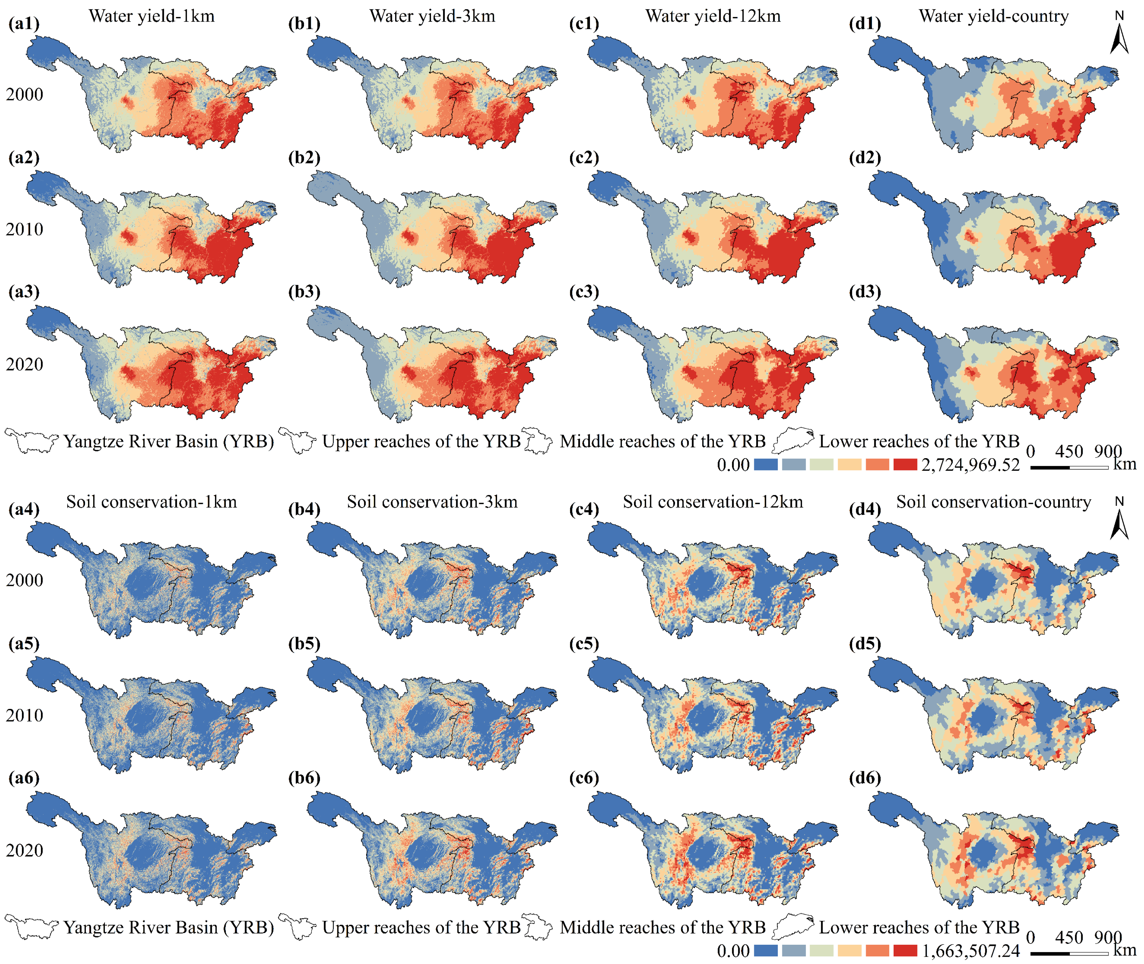
2.5. Quantifying WESs Supply

WY supply. The supply of WY was determined using the InVEST model’s yearly WY module. This module uses evapotranspiration and precipitation to estimate the WY of ecosystems, based on the theory of water balance [82].

$$SW{Y}_{(i,j)}=\left(1-{\displaystyle \frac{AE{T}_{(i,j)}}{P_{(i,j)}}}\right)\cdot P_{(i,j)}$$

(1)

where SWY_(i,j) represents the annual WY supply (mm) of pixel j in the year i, AET_(i,j) is the yearly actual evapotranspiration (mm), P_(i,j) is the annual precipitation (mm).

Supply of SC. Use the InVEST model’s sediment delivery ratio module to calculate the supply of SC. The difference between prospective and actual soil erosion was used to calculate SC using the universal soil loss equation [83].

$$\begin{array}{l}{K}_x=\left\{0.2+0.3\exp \left[-0.0256SAN(1-SIL/100)\right]\right\}\times {\left[SIL/(CLA+SIL)\right]}^{0.3}\\ \times \left\{1-0.25C/(C+e^{3.72-2.95C})\right\}\times \left(1-0.7SN1/(S{N}_1+e^{-5.51+22.9S{N}_1})\right)\end{array}$$

(2)

$$R_x=0.0534P_x^{1.6548}$$

(3)

$$RKL{S}_x=R_x\cdot K_x\cdot L{S}_x$$

(4)

$$USR{L}_x=R_x\cdot K_x\cdot L{S}_x\cdot C_x\cdot P_x$$

(5)

$$S{C}_x=RKL{S}_x-USL{E}_x$$

(6)

$$S{C}_x=R_x\cdot K_x\cdot L{S}_x\cdot \left(1-C_x\cdot P_x\right)$$

(7)

where SC_x is the supply of SC at pixel x; RKLS_x represents average annual potential soil erosion; USLE_x is the average actual yearly soil erosion; R_x is rainfall erosivity of the n-th year (MJ·mm/(hm²·h)); K_x is the soil erosion coefficient; LS_x is the field topography coefficient; C_x is the planting and management coefficient x; and P_x is the coefficient of the supporting conservation measures. In the soil particle classification standard, SAN, SIL, and CLA represent the sand, silt, and clay contents. SN₁ is calculated as 1 minus SAN divided by 100. C signifies the organic carbon content. P_x is the rainfall in the nth year (mm).

WP supply. WP services are measured by nitrogen export. The nutrient delivery ratio module in the InVEST model represents the quantity of NE.

$$N\_\exp or{t}_i=loa{d}_i-ND{R}_i+load$$

(8)

where N_export_i is the nutrient (nitrogen) export (NE) on pixel i, load_i is the modified nutrient load, and NDR_i is the nutrient delivery ratio.

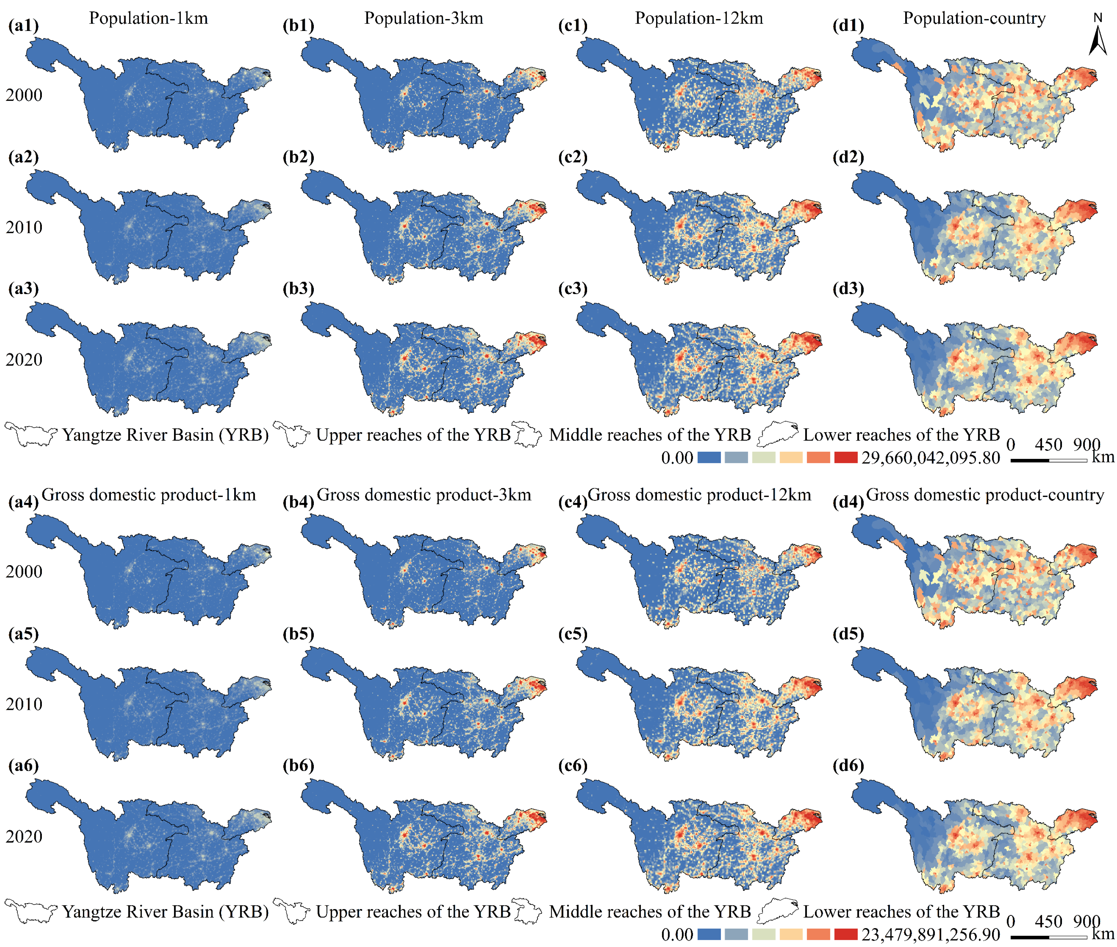
2.6. Quantifying WESs Demand

WY demand. Water resource consumption is regarded as the WY demand [84].

$$DPO{P}_{(i,j)}={\displaystyle \frac{NL{D}_{(i,j)}}{{\displaystyle {\sum }_{j=1}^{n}NL{D}_{(i,j)}}}}\cdot PO{P}_i$$

(9)

$$DGD{P}_{(i,j)}={\displaystyle \frac{NL{D}_{(i,j)}}{{\displaystyle {\sum }_{j=1}^{n}NL{D}_{(i,j)}}}}\cdot GD{P}_i$$

(10)

$$DW{Y}_{(i,j)}=DPO{P}_{(i,j)}\cdot P_i+DGD{P}_{(i,j)}\cdot G_i+DCR{O}_{(i,j)}\cdot C_i$$

(11)

where DWY_(i,j) represents the demand of WY (mm), Dpop_(i,j), and DGDP_(i,j) are the amounts of water consumed by domestic population, DCRO_(i,j) is cropland area, NLD_(i,j) was the pixel value for nighttime light, POP_i and GDP_i are the ith year values, and P_i, G_i, and C_i are per capita household water consumption, water consumption per RMB 10,000 GDP and per mu cropland irrigation consumption in the year i, respectively. Water consumption data were sourced from the China Water Resources Bulletin. Population and GDP contributions are calibrated for the ith year according to the corresponding year’s population and GDP. This study mainly considers residential and industrial water demand to calculate water demand. Therefore, rivers near industrial and residential areas may have high water demand due to the high water consumption in these places. At the same time, considering that unused land has little demand for living and production, the water demand for wasteland may be small.

SC demand. The net quantity of soil that humans seek to control and collect is referred to as actual soil erosion. Consequently, real soil erosion should be used to indicate the need for SC.

$${SC}_{dx}=USR{L}_x=R_x\cdot K_x\cdot L{S}_x\cdot C_x\cdot P_x$$

(12)

where SC_d is the demand of SC at pixel x.

WP demand. The permissible nitrogen concentration for each sub-catchment is determined by taking the goal value of the water-quality-related nitrogen concentration standard. The permissible nitrogen content for each grid is determined by multiplying the standard value of allowable nitrogen concentration by the WY; this is also known as the NE demand.

$$N\_deman{d}_i=SWY\cdot c$$

(13)

where N_demand_i is the NE demand, Y_i represents the WY (m³), c is the nitrogen concentration standard value (mg/L). Since high NE can put pressure on WP, NE can be used as a negative indicator of WP services [85].

2.7. Quantification of WESs Supply–Demand Change

Hot (Cool) Spots Identification: Hot (cool) areas do not necessarily indicate statistically significant high (low) values. The Getis-Ord Gi* tool on the ArcGIS platform has been widely applied in ecological and socio-economic environmental studies as an effective method for evaluating global clustering [86]. This tool identifies statistically significant spatial clusters of high and low values, represented as hot and cold spots [87]. In this study, the Getis-Ord Gi* hot (cold) spot analysis was employed to explore the spatial clustering and dispersal characteristics of changes in WESs supply–demand across the YRB. The tool provides insights into the geographic distribution of areas where significant concentrations of either high or low values are found, highlighting regions of interest for further ecological and resource management strategies. The basic formula for this analysis is as follows:

$$G_i^{*}={\displaystyle \frac{{\displaystyle {\sum }_{j=1}^n{w}_{ij}{x}_j-\overline{X}{\displaystyle {\sum }_{j=1}^n{w}_{ij}}}}{S\sqrt{\frac{\left[n{\displaystyle \sum _{j=1}^n{w}_{ij}^2}-{\left({\displaystyle \sum _{j=1}^n{w}_{ij}}\right)}^2\right]}{n-1}}}}$$

(14)

$$\overline{X}={\displaystyle \frac{{\displaystyle \sum _{j=1}^n{x}_j}}{n}}$$

(15)

$$S=\sqrt{{\displaystyle \frac{{\displaystyle \sum _{j=1}^n{x}_j^2}}{n}}-{(\overline{X})}^2}$$

(16)

where $G_i^{*}$ is the statistically significant z-score for the ith river basin, x_j is the attribute value of element j, w_ij is the spatial weight between the ith and jth river basin, and n is the total number of plaques.

2.8. OPGD Model and Identification of Dominant Factors

The GD is a statistical technique used to measure the collinearity among multiple independent factors about a dependent variable within a specific region. It helps identify geographically stratified heterogeneity and the driving forces behind distinct natural geographies. [88] This approach necessitates the discretization of continuous variables, with the q statistic [89] employed to assess the effects of this discretization. Historically, settings were manually configured, which could introduce bias. To address this, we utilize five discretization methods: quantile breakpoints, natural breakpoints, standard deviation breakpoints, and equal interval breakpoints. Using the R environment (R version 4.2.3), we calculate the q value for each continuous factor. To determine the optimal variable explanatory power, we examine interval numbers ranging from 3 to 20 classes [90,91]. We then select the combination of parameters (number of intervals and classification technique) that yields the highest q value for spatial discretization. The OPGD model aims to enhance accuracy and stability in detection results by optimizing model parameters through an algorithm. Using the optimized parameters from the GDM factor detection, we identify the forces influencing the distribution characteristics of the ecological system balance pattern in the YRB. The following is the equation for this process:

$$q=1-{\displaystyle \frac{SSW}{SST}}=1-{\displaystyle \frac{{\displaystyle {\sum }_{h=1}^L{N}_h{\sigma }_h^2}}{N{\sigma }^2}}$$

(17)

where q represents the explanatory power value of the independent variable for WESs supply–demand changes, SSW and SST are the variances of the sub-area for the specific factor and the total variance of all areas, respectively, h denotes the number of categories, N_h and N represent the number of evaluation units in layer h and the entire study area, respectively, and σ_h² and σ² indicate the variances of the layer and the entire study area, respectively. The q value usually ranges between −1 and 1; the larger the q value, the more significant the spatial heterogeneity of the WESs balance [92].

As shown in

Table 2. An evaluation metric for the supply–demand drivers in WESs.

Types	Sub-Types	Driving Factors	Code
Ecological factors	Terrain	Average elevation (m)	DEM
		Terrain slope	Slope
	Meteorological	Annual average precipitation (mm)	PRE
		Annual average temperature (mm)	TEM
	Vegetation	Normalized differential vegetation index	NDVI
Social factors	Population	Population density (person/km2)	POP
	Economy	Economic density (104 yuan/km2)	GDP
	Land use and land cover type	Forest land proportion (%)	FLP
		Construction land proportion (%)	COP
		Water bodies proportion (%)	WBP

, terrain, climate, vegetation, population, economics, and LULC types significantly influence the relationship between changes in ecosystem supply–demand and their spatial patterns [93,94]. Altitude and slope, as key topographical features, affect the capacity of WESs to modify supply–demand, as well as the geographical distribution of human activities [95]. Meteorological factors, such as precipitation and temperature, can alter biophysical processes and ecological systems [96]. Research shows that areas with substantial discrepancies in the NDVI provide diverse regulatory functions [97,98]. GDP and population are critical indicators of socioeconomic development [99], while LULC changes directly impact variations in WESs supply–demand [100]. Considering the natural and socioeconomic context of the YRBs, we identified 11 driving factors based on two principles: (1) data accessibility; (2) non-collinearity of variables.

2.9. Multi-Scale Geographically Weighed Regression

The benefit of MGWR is that it can take into account the diverse spatial scales of different variables on the surface in addition to capturing the geographically heterogeneous relationships between response and explanatory factors. The MGWR model is deployed and calculated using the following modeling process:

$$y_i={\displaystyle {\sum }_{j=0}^m{\beta }_{bwj}(u_i,v_i)x_{ij}+{\epsilon }_i}$$

(18)

where y_i represents ESs, x_ij represents selected driving factors, (u_i,v_i) are the locations of different samples, ${\beta }_{bwj}$ in b_wj refers to the bandwidth used to calibrate the jth conditional relationship, ${\epsilon }_i$ is the random error term.

3. Results

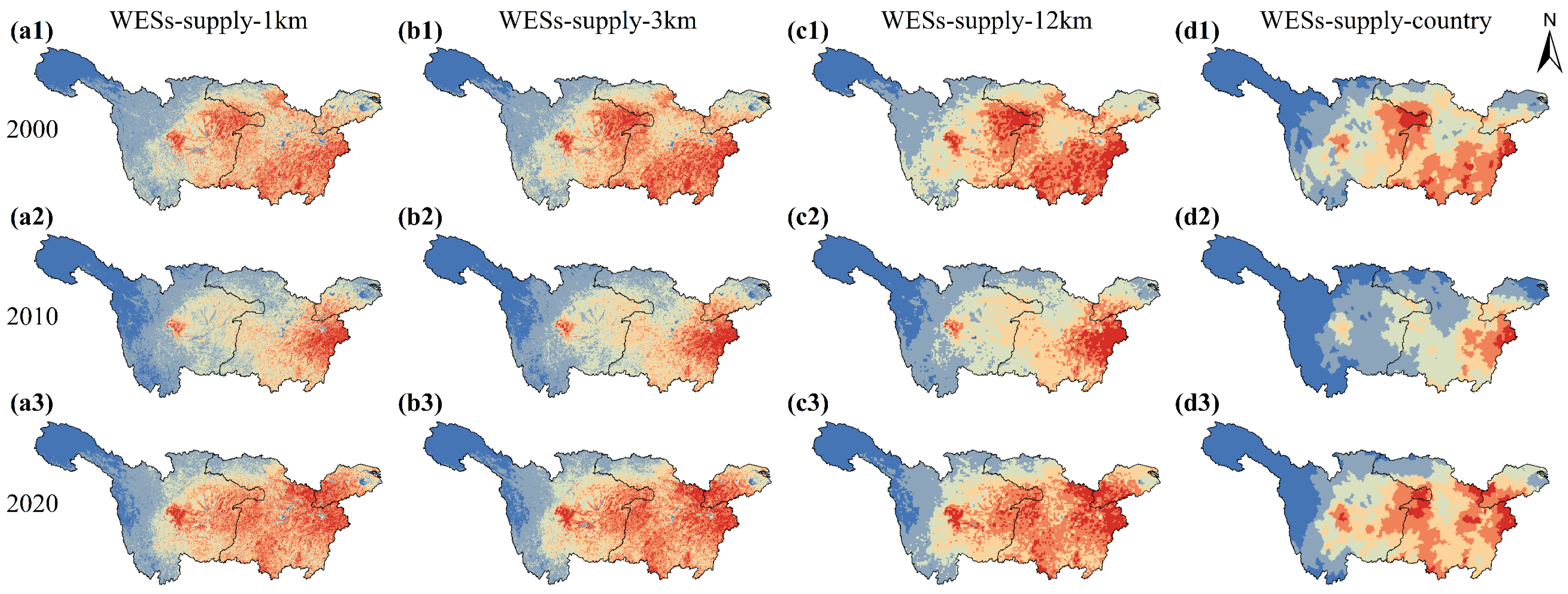
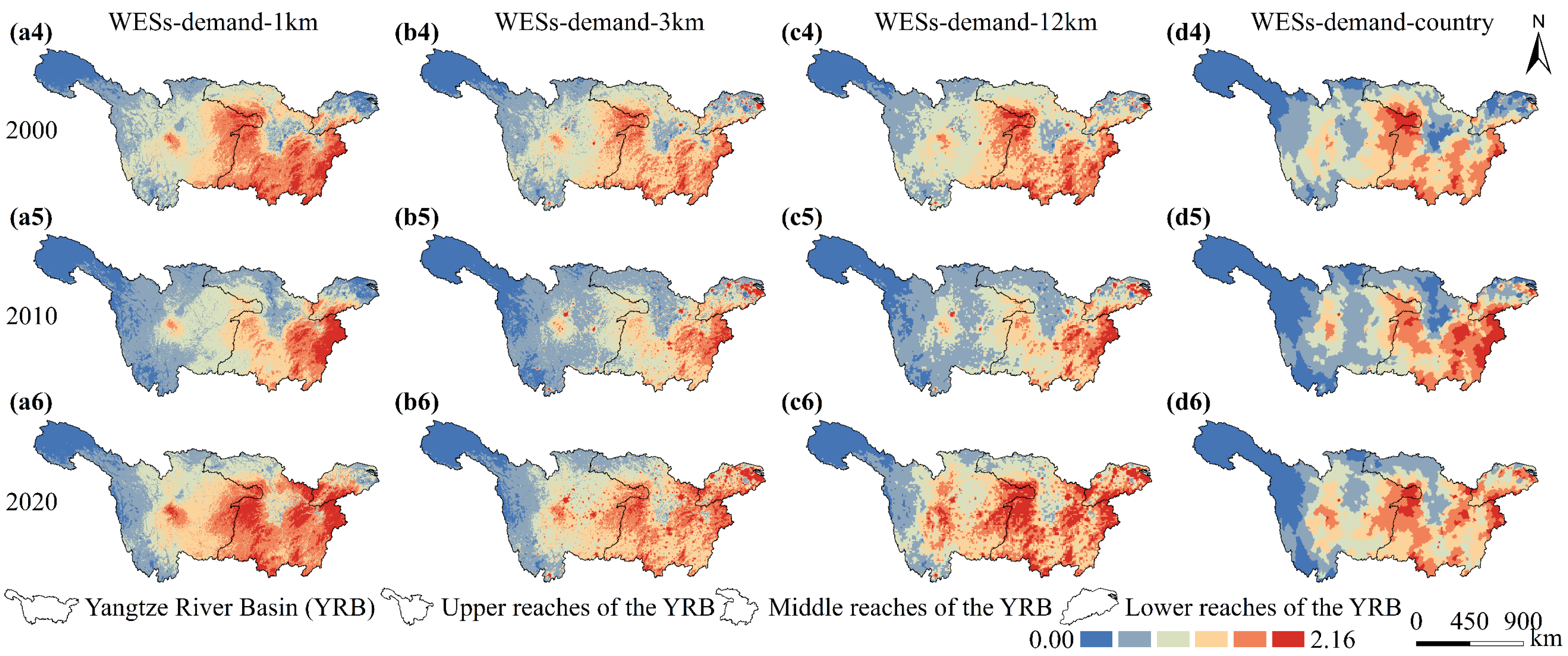
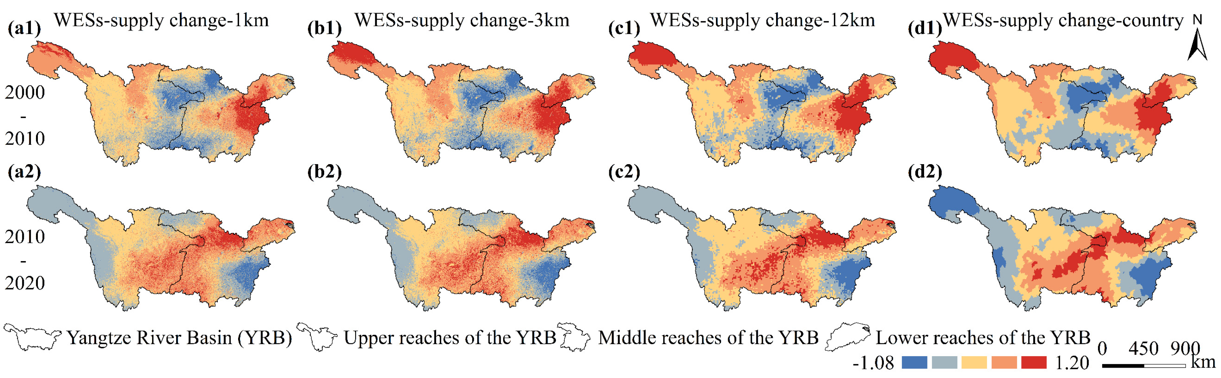
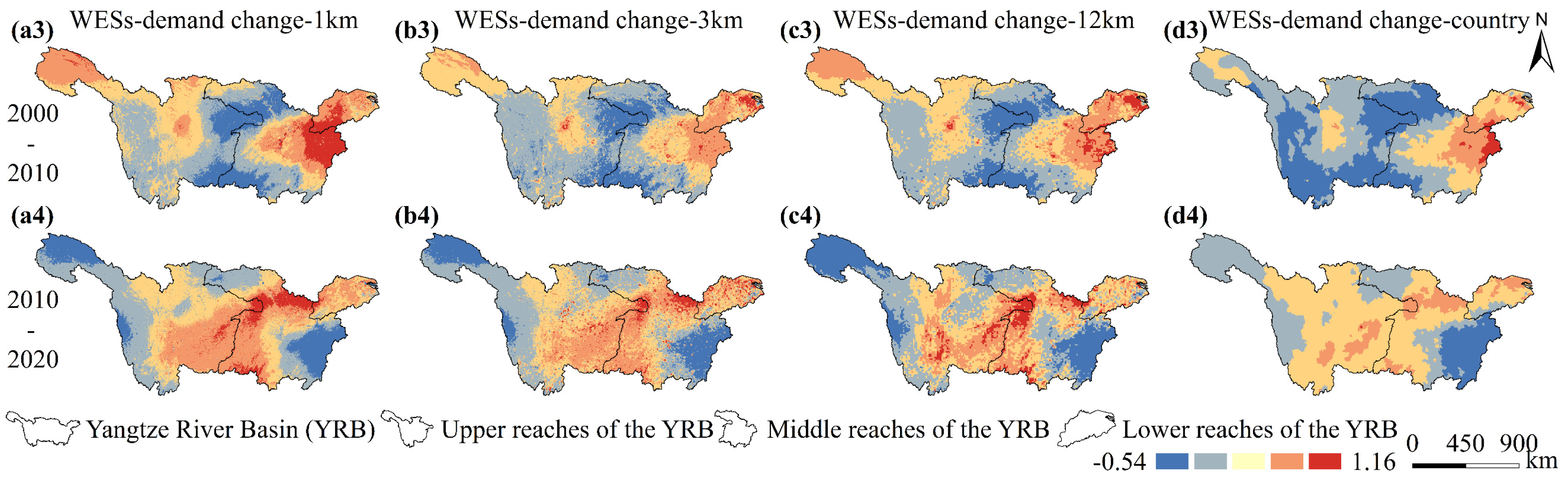
3.1. Spatial Patterns Evolution of WESs Supply–Demand Across Scales

An analysis of the temporal and geographical dynamics of various WESs from 2000 to 2020 reveals that most high-volume water supply locations are situated in the southeast of the middle reaches of the YRB (Figure 3). These high-water-supply areas have been expanding annually, with their volume increasing from 1183.40 billion m³ in 2000 to 1341.54 billion m³ in 2020. The geographical distribution aligns closely with precipitation patterns and exhibits a clustered nature. The upper reaches of the YRB contain the majority of the high-value soil retention zones, while the lower reaches are predominantly characterized by low-value areas. From 2000 to 2020, the value of high-value soil retention areas rose annually from 50.89 billion tons to 56.47 billion tons. Overall, the geographical distribution of soil retention largely reflects forest land characteristics. Additionally, the middle reaches of the YRB host most of the high-value nitrogen export zones, whereas the lower reaches are primarily associated with low-value sectors. Between 2000 and 2020, the area classified as high-value for nitrogen export increased by 1.69 billion tons, indicating a trend of progressive expansion.

A closer examination of the temporal and spatial dynamics of various WESs from 2000 to 2020 reveals a strong correlation between GDP and population distribution in the YRB. The high-value areas are predominantly concentrated in the middle and lower reaches of the YRB, with a particularly noticeable concentration in the lower reaches (Figure 4). Between 2000 and 2020, the lower reaches had an average population of 10,381,726, while the middle reaches recorded the highest GDP, averaging RMB 40.47 billion during the same period. Additionally, the area used for farming decreased, totaling 2281.157 km², of which 3.76% was allocated to residential development. The demand for soil retention is projected to rise annually, increasing from 63.48 billion tons in 2000 to 75.63 billion tons in 2020, closely aligning with the regional distribution of soil retention. Similarly, the need for WP is also growing, rising from 563,000 tons in 2000 to 624,000 tons in 2020, reflecting changes in water volume and the spatial distribution of demand.

Figure 5 presents the assessment of WESs supply across four scales in the YRB from 2000 to 2020. The eastern part of the middle reaches is home to the highest-value areas for WESs supply–demand, which are particularly concentrated in Shangrao City (Jiangxi Province), encompassing Yanshan, Yushan, and surrounding regions, as well as Leshan City (Sichuan Province), which includes Shawan, Shizhong, and adjacent areas. In the central section of the YRB, the supply–demand for high-value WESs significantly declined between 2000 and 2010; however, from 2010 to 2020, there was a notable increase in high-value locations. Throughout the lower regions of the YRB, both production and demand for high-value WESs exhibited consistent yearly growth from 2000 to 2020. Additionally, the geographical variability of WESs supply diminishes as the study scale increases, with high-value locations increasingly gravitating toward the center.

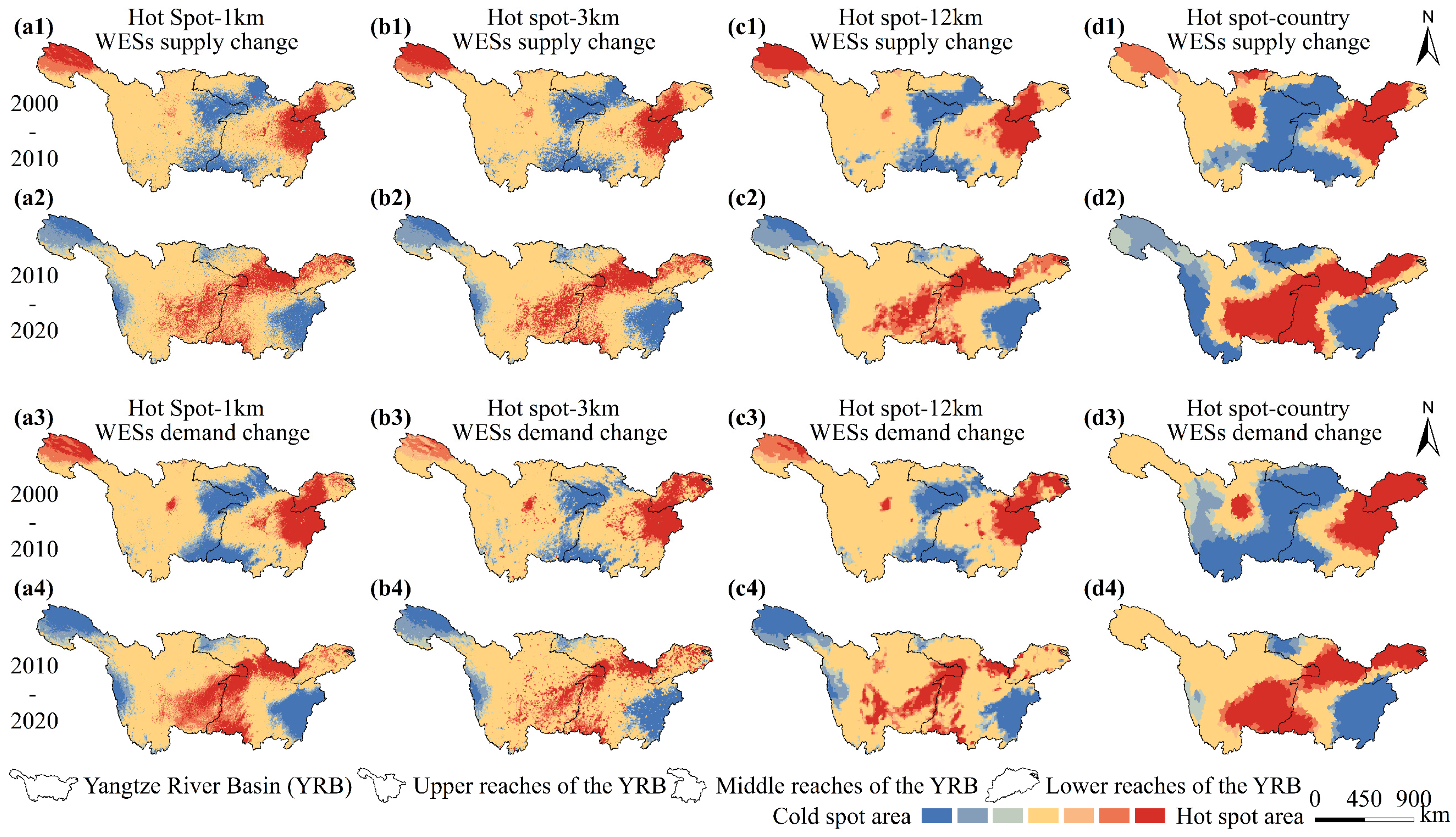
3.2. Similarities or Discrepancies in Space Between WESs Supply–Demand Fluctuations Across Several Scales

This study examined the regional patterns of changes in WESs supply–demand in the YRB between 2000 and 2020 (Figure 6). The data indicate that the area with increasing WESs supply accounted for 13.92% of the total area from 2000 to 2010 and 89.88% from 2010 to 2020. In terms of demand, the region experiencing rising demand represented 17.30% of the total demand between 2000 and 2010, increasing to 90.24% between 2010 and 2020. Notably, both supply–demand have continued to rise in the lower areas of the YRB. Analyzing the spatial aggregation features of supply–demand changes in WESs can facilitate further spatial zoning and management. There has been a significant reduction in both WESs supply and WESs demand in the southeastern part of the YRB, which stands out as a definite cold spot. In contrast, the lower sections of the YRB exhibit notable hot spot locations.

A comparison of variations in WESs supply changes among hot spot regions (three intervals), non-significant areas (one interval), and cold spot areas (three intervals) was conducted by superimposing the cold and hot spots with the changes in WESs supply–demand (Figure 7). These three categories are distinct and should not be combined, as the data reveal significant disparities in the variations of WESs supply–demand.

Using the aforementioned principles, the geographical pattern of changes in WESs supply–demand was overlaid, resulting in the categorization of 49 distinct types of WESs supply–demand variations (Figure 8). Significant changes in supply–demand between 2000 and 2020 were primarily concentrated in the lower regions of the YRB, especially in Jiangsu Province (Nanjing, Changzhou), Anhui Province (Chuzhou), and the middle reaches of Hubei Province (Huanggang, Wuhan). During this period, the middle reaches of the YRB in Shaanxi Province (Hanzhong, Shangluo) and Jiangxi Province (Ganzhou, Yingtan) experienced low supply–demand changes. Areas with minimal changes were also found in the upper reaches of the YRB in Sichuan Province (Bazhong, Dazhou), Guizhou Province (Zunyi, Bijie), and the middle reaches of Hubei Province (Shiyan, Jingmen) from 2010 to 2020. As the scale shifts from fine to coarse, the area of clusters characterized by high supply–high demand changes and low supply–low demand changes increases.

3.3. Socioecological Driving Forces of WESs Supply–Demand Changes at Multiple Scales

The data presented in

Table 3. The shares (q value) of the variables affecting the supply–demand of WESs.

Scale	1 km		3 km		12 km		County
Year	2000–2010	2010–2020	2000–2010	2010–2020	2000–2010	2010–2020	2000–2010	2010–2020
Pre	0.3190	0.4087	0.2993	0.3992	0.2458	0.3572	0.2094	0.2523
Tem	0.1492	0.1643	0.1972	0.2868	0.2266	0.3235	0.1785	0.2077
Ndvi	0.1182	0.1326	0.1192	0.1337	0.1581	0.1725	0.0879	0.1095
Cop	0.0014	0.0086	0.0099	0.0191	0.0336	0.0486	0.2166	0.2307
Clp	0.0215	0.0191	0.0672	0.1070	0.0615	0.1354	0.0614	0.0935
Flip	0.0207	0.0053	0.1253	0.0931	0.1179	0.0529	0.1301	0.0578
WBP	0.0264	0.0044	0.0339	0.0051	0.0867	0.0032	0.1867	0.0414
POP	0.0179	0.0216	0.0514	0.0996	0.1149	0.1960	0.2260	0.2685
GDP	0.0177	0.0211	0.0500	0.0990	0.1186	0.1931	0.2211	0.2708
DEM	0.1438	0.1619	0.2525	0.2519	0.2473	0.2374	0.2378	0.2012
Slope	0.0482	0.0027	0.0691	0.0250	0.0627	0.0504	0.0594	0.0556

indicate that the factors influencing the variations in WESs supply–demand within the YRB differ significantly in both intensity and type across various scales. At finer scales, climate and the DEM are the primary variables affecting WESs supply–demand fluctuations. In contrast, when examining urbanization at coarser scales, socioeconomic variables such as population, GDP, and urban area emerge as the key drivers of changes in WESs supply–demand. The impact of climate change, particularly precipitation, on WESs supply–demand variations decreases as the scale increases. Conversely, socioeconomic factors related to urbanization—such as GDP, population density, and available construction area—gain importance and become more significant at larger scales, especially at the county level. Additionally, socioeconomic variables exert the most multiplicative effect on changes in WESs supply–demand over time.

The mutual inspection findings reveal that “dual-factor enhancement” is the predominant form of interaction between two factors, suggesting that complex interactions among multiple factors contribute to the geographical heterogeneity of WESs supply–demand variations in the YRB. With a determination coefficient (q value) exceeding 0.3190, the interactive effect of precipitation with other variables significantly influences WESs supply–demand variations at finer scales. The interaction between topographic and climatic conditions and variations in WESs supply–demand is particularly noteworthy. With a q value of 0.4232, which surpasses the maximum value of any single factor’s impact, the interactive effects of socioeconomic factors related to urbanization combined with natural factors (such as topography and precipitation) gradually emerge as the most influential drivers of WESs supply–demand changes as the scale becomes coarser. This suggests that the impacts of these interactions on changes in WESs supply–demand are greater than those of individual components.

The data presented in

Table 4. The contributions (q value) of factors influencing WESs supply–demand.

			Pre	Tem	NDVI	Cop	Clp	Flip	WBP	POP	GDP	DEM	Slope
1 km	2000–2010	YRBU	0.5723	0.385	0.3521	0.0019	0.1871	0.0667	0.0191	0.0044	0.0032	0.4264	0.0349
		YRBM	0.3633	0.2107	0.0209	0.0065	0.006	0.0022	0.0297	0.0122	0.0127	0.1913	0.0249
		YRBL	0.3348	0.0024	0.0449	0.0625	0.0687	0.0584	0.0180	0.1007	0.1002	0.0421	0.0698
	2000–2020	YRBU	0.5233	0.2107	0.3209	0.0075	0.006	0.0022	0.0297	0.0062	0.0067	0.4913	0.0249
		YRBM	0.3557	0.1289	0.0186	0.0118	0.0166	0.0064	0.0038	0.0143	0.0141	0.1998	0.0038
		YRBL	0.2316	0.0293	0.0187	0.0815	0.0542	0.0163	0.0703	0.1144	0.1141	0.0368	0.0108
3 km	2000–2010	YRBU	0.5769	0.3166	0.325	0.0043	0.2084	0.1647	0.0196	0.0244	0.0278	0.3606	0.0836
		YRBM	0.3363	0.2753	0.0462	0.0172	0.0343	0.1211	0.0377	0.031	0.0321	0.1682	0.0536
		YRBL	0.2995	0.2323	0.0381	0.0783	0.1171	0.0878	0.0247	0.1557	0.1509	0.0379	0.0939
	2000–2020	YRBU	0.5187	0.4118	0.3918	0.015	0.2559	0.1547	0.024	0.0908	0.0887	0.4524	0.0608
		YRBM	0.3241	0.3247	0.0298	0.0244	0.0341	0.1374	0.0073	0.0929	0.093	0.1363	0.0278
		YRBL	0.2767	0.0909	0.0373	0.0928	0.1443	0.0681	0.0463	0.1674	0.171	0.0482	0.0365
12 km	2000–2010	YRBU	0.5733	0.4119	0.4629	0.0285	0.2811	0.3299	0.0845	0.0984	0.1166	0.4409	0.1518
		YRBM	0.3212	0.2934	0.0502	0.0542	0.0382	0.0274	0.085	0.1226	0.1257	0.2038	0.0778
		YRBL	0.2979	0.2316	0.0548	0.1332	0.0339	0.1095	0.0309	0.2675	0.2696	0.1293	0.0931
	2000–2020	YRBU	0.5372	0.4571	0.4773	0.0841	0.3541	0.2792	0.0569	0.1523	0.1504	0.5131	0.0949
		YRBM	0.3086	0.3503	0.0253	0.1161	0.0375	0.0361	0.0077	0.1733	0.1776	0.0609	0.0491
		YRBL	0.2877	0.1585	0.0202	0.2296	0.0587	0.0291	0.0288	0.2630	0.2757	0.0503	0.0539
County	2000–2010	YRBU	0.3352	0.2592	0.227	0.1154	0.1751	0.1988	0.0485	0.1152	0.1216	0.3433	0.2271
		YRBM	0.2673	0.2350	0.1104	0.1668	0.0496	0.0646	0.2312	0.1796	0.1997	0.1981	0.165
		YRBL	0.1814	0.2247	0.2098	0.2219	0.1094	0.1667	0.1189	0.3328	0.3366	0.1087	0.1373
	2000–2020	YRBU	0.3172	0.2790	0.2205	0.1296	0.1554	0.1631	0.0211	0.1669	0.1689	0.3490	0.2415
		YRBM	0.2518	0.2510	0.1521	0.1800	0.0767	0.0646	0.0407	0.2364	0.2345	0.1972	0.0781
		YRBL	0.1361	0.2194	0.1429	0.2351	0.1404	0.0963	0.1361	0.3497	0.3597	0.1008	0.1620

YRBU: the upper reaches of the YRB; YRBM: the middle reaches of the YRB; YRBL: the lower reaches of the YRB.

indicate that the degree of impact from various factors changes across different periods and scales for distinct basins. At the same time and scale, the influence of climate variables (temperature and precipitation) and the DEM on variations in WESs supply–demand gradually diminishes from the higher to the middle, and finally to the lower reaches of the YRB. Conversely, the impact of urbanization-related socioeconomic variables, such as population, building area, and economic factors, steadily increases. As economic growth and urbanization progress, the influence of meteorological variables (temperature and precipitation) on WESs supply–demand across basins decreases, while the significance of socioeconomic variables associated with urbanization (such as building area, GDP, and population) rises. Additionally, the DEM and climate change have a more pronounced impact on WESs supply–demand fluctuations at smaller scales. In the lower reaches of the YRB, the influence of construction land surpasses that of climatic factors at the county level, where socioeconomic factors related to urbanization become the primary drivers of WESs supply–demand changes, especially at coarser scales.

The mutual inspection results further reveal that topography and climate are the main variables affecting fluctuations in WESs supply–demand in the upper and middle reaches of the YRB. In the lower reaches, climate and urbanization-related socioeconomic variables are the primary forces influencing these variations. Furthermore, the influence of urbanization-related socioeconomic and climatic variables on changes in WESs supply–demand intensifies at coarser scales.

3.4. The Main Forces Impacting the Supply–Demand of WESs Expressed Spatially

This study uses the MGWR model for analysis to investigate the regional heterogeneity of the effects of anthropogenic and natural influences on the ecological environment. To get rid of duplicate variables, a covariance test on the explanatory variables is required before using the MGWR model. In this study, we find the Variance Inflation Factor (VIF) for each variable using the RStudio (Version 4.3.2) software’s Car package. There are no duplicate variables as each factor’s VIF value is less than 10.

To find the model that fits the data the best, we compared the MGWR model with the OLS model. The Residual Sum of Squares (RSS), modified R2, R2, and Akaike Information Criterion (AIC) are among the diagnostic measures. Model performance is measured by the Corrected Akaike Information Criterion (AICc), where a lower AICc value denotes greater performance [101,102]. Of the models that were examined, the GWR model suited the data better than the OLS model, as evidenced by its lower RSS and AICc values as well as higher R2 and modified R2 values.

The DEM mostly harms variations in WESs supply–demand (Figure 9). Slope mostly has a beneficial impact on variations in WESs supply–demand. Rainfall affects WESs supply–demand fluctuations in both positive and negative ways, contributing 60.91% and 39.09% of the YRB, respectively. Temperature significantly affects how WESs supply–demand fluctuate. The supply–demand fluctuations in WESs, which account for 44.58% and 55.42% of the YRB, respectively, are positively and adversely impacted by the NDVI. Positive and negative effects on changes in WESs supply–demand are accounted for by the COP area, which accounts for 49.27% and 50.73% of the YRB, respectively. FLP mostly has a negative effect on changes in WESs supply–demand. WBP mostly has a beneficial impact on changes in WESs supply–demand. Population growth primarily has a negative influence on changes in WESs supply–demand, but economic growth primarily has a positive impact.

4. Discussion

4.1. The Supply–Demand Patterns and Connections of WESs Vary at Different Sizes

The supply capacity of the ecosystem, demand patterns and the dynamic equilibrium between supply–demand have all been significantly impacted by the geographical variability of socio-ecological elements and their divergences at various levels. Consequently, ESs show complex spatiotemporal fluctuations at different scales. To promote the harmonious development of ecology and civilization, it is essential to delve into the supply–demand dynamics of WESs at various scales and incorporate them into the environmental decision-making process. In certain developed counties or smaller patches, supply–demand mismatches persist even though some isolated provinces and counties can become self-sufficient in important WESs. Consequently, ongoing optimization and increased focus on finer management levels are necessary for the ecological and environmental management of the YRB. When examined at a finer grid size, deficit patches typically enlarge from central cities into outlying regions.

Rather than being evenly distributed, some studies have demonstrated that WESs show a significant degree of agglomeration within different landscapes [103]. WESs often show more intricate spatial patterns at the microscale; however, as the scale grows, the effects of spatial aggregation cause these patterns to become more uniform at the macroscale [104]. As a result, there are notable variations in the county size, but overall, the supply–demand spatial patterns across the three grid scales in the YRB are rather comparable. This result is in line with studies performed in Quebec, Canada, where there was significant variance with larger sizes but equivalent geographic patterns of ESs supply at lower scales. Additionally, it was noted by Baró et al. [105] that there is a greater similarity in supply–demand patterns across township and cell scales as compared to county sizes. However, all scales exhibit the prevalence of spatial mismatch types (e.g., H-L and L-H), which is in line with the results of different research [106]. The results show that there are ecological fluxes because of the way in which supply–demand are distributed geographically. This emphasizes how important it is to concentrate management efforts when developing conservation or restoration plans in regions where there are mismatches. Scale effects result from changes in the composition of LULC under various assessment scales, which have a substantial impact on the geographical patterns and matching relationships of supply–demand for WESs. Each observation unit at the finer grid sizes usually shows just one type of LULC, and the strong demand for WESs frequently results in a deficit in the building land grid. However, as the scale grows, the LULC kinds inside each unit gradually become more diverse, and the amount of ecological land areas that may supply WESs, including woods, grasslands, and water bodies, rises in the vicinity of building sites. This phenomenon emphasizes how important it is to show spatial patterns and supply–demand relationships at different scales. This helps to avoid overestimating the supply capacity of WESs at finer scales because of averaging effects, and it also helps to understand overall trends at coarser scales. It is noteworthy that when we proceed to coarser scales, the supply–demand dynamics of WESs inside the YRB tend to become less concentrated. This issue occurs because discrete clusters may be exposed to interpolation or truncation on the map as a result of the so-called “shaving” effect when data are aggregated to larger sizes [107]. To sum up, by utilizing the benefits of various scales, a multi-scale evaluation of WESs supply–demand may offer more accurate assistance for spatial decision-making.

4.2. Impact of Human and Natural Factors on WESs

Climate variables are the primary drivers of WESs, as indicated by the OPGD model at the fine scale. According to single-factor tests, PRE (0.3639) and TEM (0.1568) have the greatest impact on the spatiotemporal differentiation of WESs in the YRB at this scale. This is consistent with previous research [108] that shows PRE and TEM as the primary drivers of regional spatiotemporal differentiation of WESs. On the other hand, PRE and DEM become dominant variables influencing the spatiotemporal variance of WESs in the YRB when the scale moves to coarser levels. The primary drivers of the spatiotemporal differentiation of WESs at the county level are human activities, such as GDP and POP. In keeping with these results, our multi-year comparisons show that human factors have had a greater influence on WESs over time, which is consistent with the viewpoints presented by Chen et al. [109]. Unusual variations in WY and SC are the consequence of changes in surface runoff and sediment transport brought about by the growth of urban impervious surfaces. The demand for WESs has increased dramatically along with the acceleration of urbanization and fast population development, placing a significant strain on ecosystems. For instance, Wu et al.‘s research [110] shows that Shanghai’s WESs value has been trending lower in tandem with the city’s economic and demographic expansion. Close to the city center, there is an acceleration of the fall in the value of WESs, particularly in light of the increasing urbanization of the region. The interaction of different influencing variables increases the overall effect of those elements on WESs. At various times, aspect, NDVI, and EVP alone have less of an impact on WESs; but when combined with meteorological variables such as TEM and PRE, they strengthen their explanatory ability. For example, when the TEM factor and PRE are combined, their synergistic impact is significantly greater than when they are used alone (TEM ∩ PRE = PRE). The fluctuations in WESs (PRE ∩ POP > POP, TEM ∩ POP = POP) are influenced by the interplay between human activity and environmental factors. These interactions often amplify the impacts of human activity. This outcome is consistent with the opinions stated by Birk and colleagues [111]. The MGWR model provides more sophisticated geographical visualization and clarifies the methods by which primary driving variables impact WESs more precisely than OLS and GWR. The MGWR model’s coefficients not only show the geographical heterogeneity relationships between the driving elements that finally lead to the selection of WESs, but they also offer crucial information for local ecological planning. Additionally, the spatial balance between the natural supply and the societal demand on the local biological environment is greatly enhanced by this approach.

Studies have shown that in river basins, human influences negatively impact WESs. According to this research, human activities harm WESs more severely the more intense they are. However, via the use of techniques like afforestation that save water and soil, humans may actively increase the supply of WESs [112]. As a result, we must strictly limit human involvement, wisely distribute watershed land resources, improve the effectiveness of LULC, and further hone its structure. For example, certain vacant properties in and around cities can be developed into green areas. The terrain’s slope affects WESs in both favorable and unfavorable ways. An elevated coefficient might be strongly linked to the complex impacts of terrain distortion on water-evaporation systems. By influencing the natural supply and social demand of ecosystems, geomorphological factors control the geographical pattern of ecosystem supply–demand coordination. For instance, slope and elevation have a direct impact on biophysical parameters, including temperature, evapotranspiration, moisture content, and soil type, which eventually causes the spatial variability of WESs. PRE has a beneficial effect on WESs, and earlier research has also shown that precipitation significantly improves WESs. Overall, from east to west, PRE’s beneficial effects on WESs progressively decrease. It is possible to implement several effective and regionally focused ecological protection strategies in light of the study findings presented above. In the higher reaches of the YRB, for instance, encouraging the establishment of drought and water-resistant plant species can both improve the quality of WESs and satisfy human demand for recreational spaces.

4.3. Policy Impacts

The environmental carrying capacity and economic growth tendencies of each region must be completely taken into account while developing financial plans and putting ecological protection measures into action. In the basin, increasingly large areas are being set aside for urbanization at the same time as the availability of water resources is declining. The population’s constant growth is progressively overtaking the natural environment, and water shortage has emerged as a major barrier to basin development. Furthermore, while urbanization has promoted economic expansion, environmental problems have also resulted from it. The main causes of harm to regional ecosystems are pollution emissions and the ecological effects of LULC [113]. On the other hand, ecological-degradation-related environmental problems might also somewhat impede urban growth [114].

The results of this research indicate that natural processes continue to be the dominant forces behind the geographical patterns of ecosystem changes in the basin, even though human actions may also have an impact on the sustainability of basin ecosystems. The ecology has been negatively impacted by the growth of megacities, which has increased environmental strain. Consequently, initiatives to drive the basin’s future growth should place a high priority on preserving the environment, carrying out land restoration initiatives like “converting agriculture to forest” in strategic locations and actively supporting green development. The coordinated development of the environment, society, and economy; the creation of a socioeconomic structure that is environmentally friendly and serves the public interest; and the achievement of sustainable development—the peaceful coexistence of the environment and the economy—should be the main goals of environmental protection initiatives.

4.4. Comparisons with Previous Studies

This study distinguishes itself from previous research on ESs supply–demand by utilizing long-term multi-source remote sensing data to validate and summarize the mechanisms influencing various landscape watersheds across multiple spatial scales. It clarifies the factors driving the evolution of WESs supply–demand and their spatial heterogeneity, providing a scientific foundation for ecological protection measures at different scales. Furthermore, by integrating the OPGD and MGWR models, this research addresses gaps in prior studies regarding the driving factors influencing the spatial heterogeneity of WESs. Through enhanced spatial representation, it offers a thorough analysis of the key driving factors affecting the supply–demand of these ecosystems, deepening the understanding of these influences across diverse watershed characteristics.

Compared to existing research on the supply–demand of WESs, this study’s primary innovation lies in its scientific rigor, comparability, suitability, replicability, clarity, and objectivity, allowing for a systematic exploration of the evolution and driving mechanisms of WESs supply–demand at both macro and local scales. First, this study selects essential factors and scales related to WESs, providing a solid scientific foundation for the research. Second, while previous supply–demand assessments have often been difficult to compare and validate, this study observes varying degrees of impact from natural and anthropogenic factors on WESs across different temporal and spatial scales through long-term sequential changes and multi-scale, multi-regional comparisons. Third, the OPGD method utilizes the highest q-value combinations of categorical parameters to discretize continuous variables, effectively overcoming human subjectivity while enhancing the quantitative analysis of driving mechanisms in WESs. Fourth, the MGWR method employed helps to visually demonstrate the effects of driving factors on WESs across different spatial scales. Lastly, the methodological framework of this study exhibits strong adaptability and portability, proving that OPGD and MGWR can be applied to the analysis of WESs in other research areas.

4.5. Limitations and Prospects

While this study’s evaluation of the mismatch between WESs supply–demand across various geographical scales has provided valuable insights into ecosystem sustainability, several issues remain unresolved. This study relied on population density to determine WESs demand; however, this approach did not adequately account for the preferences of different demographic groups (e.g., individuals of varying age groups and those in different geographical locations) due to the lack of more precise socio-economic data. Therefore, comprehensive research that considers regional variations is necessary to develop a more accurate and scientific method for evaluating WESs demand, as well as to establish a more extensive database to ensure the reliability of these evaluations. Future studies should explore diverse methods for recognizing ecological fluxes.

5. Conclusions

This research leverages long-term, multi-scale remote sensing datasets and integrates the OPGD and MGWR analytical frameworks to explore the intricate effects of various sub-basins on WESs across multiple basin scales. Furthermore, it compares regional disparities based on robust scientific hypotheses. The findings reveal that, on a panoramic scale, the overall WESs have exhibited a consistent upward trajectory during the examined years. From 2000 to 2020, total WY increased by 158.1352 billion m³; SC rose by 55.79 billion tons; and NE grew by 0.55 million tons. Through meticulous comparative analysis of long-term driving forces, it becomes evident that natural factors, particularly precipitation, exert a more significant influence on WESs at smaller scales compared to anthropogenic factors. As the research scale expands, the influence of human factors, such as GDP, gradually surpasses that of natural factors. Moreover, the growth rate of human factors over time outpaces that of climate change. Notably, a pattern emerges where the explanatory power of a single factor tends to increase when it interacts with other factors. Additionally, it is observed that the positive impact of natural factors on the southern part of the watershed decreases from east to west. Conversely, the negative effects of human factors are particularly pronounced in densely populated areas in the southern part of the watershed, indicating an uneven spatial distribution. These research results demonstrate that integrating long-term multi-scale remote sensing data with OPGD and MGWR models is an effective and practical approach for uncovering the driving forces behind changes in WESs supply–demand in complex geographical environments.

References

1. Bennett, E.M.; Baird, J.; Baulch, H.; Chaplin-Kramer, R.; Fraser, E.; Loring, P.; Morrison, P.; Parrott, L.; Sherren, K.; Winkler, K.J.; et al. Ecosystem services and the resilience of agricultural landscapes. In Advances in Ecological Research; Academic Press: Cambridge, MA, USA, 2021; Volume 64, pp. 1–43. [Google Scholar] [CrossRef]
2. Zhang, C.; Li, J.; Zhou, Z. Ecosystem service cascade: Concept, review, application and prospect. Ecol. Indic. 2022, 137, 108766. [Google Scholar] [CrossRef]
3. Zhang, Y.; Hu, W.; Liu, T.; Liu, F.; Li, S.; Zhang, S. Integrating ecosystem integrity and ES supply–demand process to explore ecological connectivity in Wuhan metropolitan area, China. Ecol. Indic. 2024, 163, 112128. [Google Scholar] [CrossRef]
4. Jiang, W.; Tan, Y. Overview on failures of urban underground infrastructures in complex geological conditions due to heavy rainfall in China during 1994–2018. Sustain. Cities Soc. 2022, 76, 103509. [Google Scholar] [CrossRef]
5. Angell, L.C.; Klassen, R.D. Integrating environmental issues into the mainstream: An agenda for research in operations management. J. Oper. Manag. 1999, 17, 575–598. [Google Scholar] [CrossRef]
6. Watson, V. ‘The planned city sweeps the poor away…’: Urban planning and 21st century urbanisation. Prog. Plan. 2009, 72, 151–193. [Google Scholar] [CrossRef]
7. Wu, J. Urban ecology and sustainability: The state-of-the-science and future directions. Landsc. Urban Plan. 2014, 125, 209–221. [Google Scholar] [CrossRef]
8. Gao, J.; Li, F.; Gao, H.; Zhou, C.; Zhang, X. The impact of land-use change on water-related ecosystem services: A study of the Guishui River Basin, Beijing, China. J. Clean. Prod. 2017, 163, S148–S155. [Google Scholar] [CrossRef]
9. Pettinotti, L.; de Ayala, A.; Ojea, E. Benefits from water related ecosystem services in Africa and climate change. Ecol. Econ. 2018, 149, 294–305. [Google Scholar] [CrossRef]
10. Li, J.; Zhou, K.; Xie, B.; Xiao, J. Impact of landscape pattern change on water-related ecosystem services: Comprehensive analysis based on heterogeneity perspective. Ecol. Indic. 2021, 133, 108372. [Google Scholar] [CrossRef]
11. Jiang, Y.; Ouyang, B.; Yan, Z. Multiscale Analysis for Identifying the Impact of Human and Natural Factors on Water-Related Ecosystem Services. Sustainability 2024, 16, 1738. [Google Scholar] [CrossRef]
12. Spangenberg, J.H. Biodiversity pressure and the driving forces behind. Ecol. Econ. 2007, 61, 146–158. [Google Scholar] [CrossRef]
13. Gobinath, R.; Ganapathy, G.P.; Gayathiri, E.; Salunkhe, A.A.; Pourghasemi, H.R. Ecoengineering practices for soil degradation protection of vulnerable hill slopes. In Computers in Earth and Environmental Sciences; Elsevier: Amsterdam, The Netherlands, 2022; pp. 255–270. [Google Scholar] [CrossRef]
14. Shannon, M.A.; Bohn, P.W.; Elimelech, M.; Georgiadis, J.G.; Mariñas, B.J.; Mayes, A.M. Science and technology for water purification in the coming decades. Nature 2008, 452, 301–310. [Google Scholar] [CrossRef] [PubMed]
15. Trivedi, P.; Wallenstein, M.D.; Delgado-Baquerizo, M.; Singh, B.K. Microbial modulators and mechanisms of soil carbon storage. In Soil Carbon Storage; Academic Press: Cambridge, MA, USA, 2018; pp. 73–115. [Google Scholar] [CrossRef]
16. Kumar, P.; Brondizio, E.; Gatzweiler, F.; Gowdy, J.; de Groot, D.; Pascual, U.; Reyers, B.; Sukhdev, P. The economics of ecosystem services: From local analysis to national policies. Curr. Opin. Environ. Sustain. 2013, 5, 78–86. [Google Scholar] [CrossRef]
17. Lyu, R.; Clarke, K.C.; Zhang, J.; Feng, J.; Jia, X.; Li, J. Spatial correlations among ecosystem services and their socio-ecological driving factors: A case study in the city belt along the Yellow River in Ningxia, China. Appl. Geogr. 2019, 108, 64–73. [Google Scholar] [CrossRef]
18. Wang, L.; Chen, C.; Xie, F.; Hu, Z.; Zhang, Z.; Chen, H.; He, X.; Chu, Y. Estimation of the value of regional ecosystem services of an archipelago using satellite remote sensing technology: A case study of Zhoushan Archipelago, China. Int. J. Appl. Earth Obs. Geoinf. 2021, 105, 102616. [Google Scholar] [CrossRef]
19. MacAlister, C.; Mahaxay, M. Mapping wetlands in the Lower Mekong Basin for wetland resource and conservation management using Landsat ETM images and field survey data. J. Environ. Manag. 2009, 90, 2130–2137. [Google Scholar] [CrossRef]
20. Milder, J.C.; Hart, A.K.; Dobie, P.; Minai, J.; Zaleski, C. Integrated landscape initiatives for African agriculture, development, and conservation: A region-wide assessment. World Dev. 2014, 54, 68–80. [Google Scholar] [CrossRef]
21. Brown, G.; Fagerholm, N. Empirical PPGIS/PGIS mapping of ecosystem services: A review and evaluation. Ecosyst. Serv. 2015, 13, 119–133. [Google Scholar] [CrossRef]
22. Jain, M.; Korzhenevych, A.; Basu, A.M. Integrating spatial development with infrastructure provision along an envisioned transport corridor: A conceptual framework and its application to India. Land Use Policy 2021, 104, 105364. [Google Scholar] [CrossRef]
23. Wang, J.; Zhai, T.; Lin, Y.; Kong, X.; He, T. Spatial imbalance and changes in supply and demand of ecosystem services in China. Sci. Total Environ. 2019, 657, 781–791. [Google Scholar] [CrossRef]
24. Guan, Q.; Hao, J.; Ren, G.; Li, M.; Chen, A.; Duan, W.; Chen, H. Ecological indexes for the analysis of the spatial–temporal characteristics of ecosystem service supply and demand: A case study of the major grain-producing regions in Quzhou, China. Ecol. Indic. 2020, 108, 105748. [Google Scholar] [CrossRef]
25. Xu, Z.; Wei, H.; Dong, X.; Liu, Y.; Xue, H. Evaluating the ecological benefits of plantations in arid areas from the perspective of ecosystem service supply and demand-based on emergy analysis. Sci. Total Environ. 2020, 705, 135853. [Google Scholar] [CrossRef]
26. Sun, X.; Tang, H.; Yang, P.; Hu, G.; Liu, Z.; Wu, J. Spatiotemporal patterns and drivers of ecosystem service supply and demand across the conterminous United States: A multiscale analysis. Sci. Total Environ. 2020, 703, 135005. [Google Scholar] [CrossRef] [PubMed]
27. Xu, X.; Chen, M.; Yang, G.; Jiang, B.; Zhang, J. Wetland ecosystem services research: A critical review. Glob. Ecol. Conserv. 2020, 22, e01027. [Google Scholar] [CrossRef]
28. Zhu, Z.; Wang, K.; Lei, M.; Li, X.; Li, X.; Jiang, L.; Gao, X.; Li, S.; Liang, J. Identification of priority areas for water ecosystem services by a techno-economic, social and climate change modeling framework. Water Res. 2022, 221, 118766. [Google Scholar] [CrossRef]
29. McNie, E.C. Reconciling the supply of scientific information with user demands: An analysis of the problem and review of the literature. Environ. Sci. Policy 2007, 10, 17–38. [Google Scholar] [CrossRef]
30. Sorrell, S. Reducing energy demand: A review of issues, challenges and approaches. Renew. Sustain. Energy Rev. 2015, 47, 74–82. [Google Scholar] [CrossRef]
31. Xu, Z.; Peng, J.; Dong, J.; Liu, Y.; Liu, Q.; Lyu, D.; Qiao, R.; Zhang, Z. Spatial correlation between the changes of ecosystem service supply and demand: An ecological zoning approach. Landsc. Urban Plan. 2022, 217, 104258. [Google Scholar] [CrossRef]
32. Mereta, S.T.; Boets, P.; Bayih, A.A.; Malu, A.; Ephrem, Z.; Sisay, A.; Endale, H.; Yitbarek, M.; Jemal, A.; De Meester, L.; et al. Analysis of environmental factors determining the abundance and diversity of macroinvertebrate taxa in natural wetlands of Southwest Ethiopia. Ecol. Inform. 2012, 7, 52–61. [Google Scholar] [CrossRef]
33. Li, J.; Xie, B.; Gao, C.; Zhou, K.; Liu, C.; Zhao, W.; Xiao, J.; Xie, J. Impacts of natural and human factors on water-related ecosystem services in the Dongting Lake Basin. J. Clean. Prod. 2022, 370, 133400. [Google Scholar] [CrossRef]
34. Saleth, R.M.; Dinar, A. Institutional changes in global water sector: Trends, patterns, and implications. Water Policy 2000, 2, 175–199. [Google Scholar] [CrossRef]
35. Goldman, M. How “Water for All!” policy became hegemonic: The power of the World Bank and its transnational policy networks. Geoforum 2007, 38, 786–800. [Google Scholar] [CrossRef]
36. Ison, R.; Röling, N.; Watson, D. Challenges to science and society in the sustainable management and use of water: Investigating the role of social learning. Environ. Sci. Policy 2007, 10, 499–511. [Google Scholar] [CrossRef]
37. Green, B. The flaws of policies requiring human oversight of government algorithms. Comput. Law Secur. Rev. 2022, 45, 105681. [Google Scholar] [CrossRef]
38. Geijzendorffer, I.R.; Martín-López, B.; Roche, P.K. Improving the identification of mismatches in ecosystem services assessments. Ecol. Indic. 2015, 52, 320–331. [Google Scholar] [CrossRef]
39. Yang, S.; Bai, Y.; Alatalo, J.M.; Wang, H.; Jiang, B.; Liu, G.; Chen, J. Spatio-temporal changes in water-related ecosystem services provision and trade-offs with food production. J. Clean. Prod. 2021, 286, 125316. [Google Scholar] [CrossRef]
40. Wang, Y.; Wang, H.; Zhang, J.; Liu, G.; Fang, Z.; Wang, D. Exploring interactions in water-related ecosystem services nexus in Loess Plateau. J. Environ. Manag. 2023, 336, 117550. [Google Scholar] [CrossRef] [PubMed]
41. Bagstad, K.J.; Johnson, G.W.; Voigt, B.; Villa, F. Spatial dynamics of ecosystem service flows: A comprehensive approach to quantifying actual services. Ecosyst. Serv. 2013, 4, 117–125. [Google Scholar] [CrossRef]
42. He, G.; Zhang, L.; Wei, X.; Jin, G. Scale effects on the supply–demand mismatches of ecosystem services in Hubei Province, China. Ecol. Indic. 2023, 153, 110461. [Google Scholar] [CrossRef]
43. Xue, C.; Xue, L.; Chen, J.; Tarolli, P.; Chen, X.; Zhang, H.; Qian, J.; Zhou, Y.; Liu, X. Understanding driving mechanisms behind the supply-demand pattern of ecosystem services for land-use administration: Insights from a spatially explicit analysis. J. Clean. Prod. 2023, 427, 139239. [Google Scholar] [CrossRef]
44. Baró, F.; Haase, D.; Gómez-Baggethun, E.; Frantzeskaki, N. Mismatches between ecosystem services supply and demand in urban areas: A quantitative assessment in five European cities. Ecol. Indic. 2015, 55, 146–158. [Google Scholar] [CrossRef]
45. Liu, H.; Xiao, W.; Zhu, J.; Zeng, L.; Li, Q. Urbanization intensifies the mismatch between the supply and demand of regional ecosystem services: A large-scale case of the Yangtze River Economic Belt in China. Remote Sens. 2022, 14, 5147. [Google Scholar] [CrossRef]
46. Wang, L.J.; Gong, J.W.; Ma, S.; Wu, S.; Zhang, X.; Jiang, J. Ecosystem service supply–demand and socioecological drivers at different spatial scales in Zhejiang Province, China. Ecol. Indic. 2022, 140, 109058. [Google Scholar] [CrossRef]
47. Qi, F.; Liu, J.; Gao, H.; Fu, T.; Wang, F. Characteristics and spatial–temporal patterns of supply and demand of ecosystem services in the Taihang Mountains. Ecol. Indic. 2023, 147, 109932. [Google Scholar] [CrossRef]
48. Sarstedt, M.; Ringle, C.M.; Hair, J.F. Partial least squares structural equation modeling. In Handbook of Market Research; Springer International Publishing: Cham, Switzerland, 2021; pp. 587–632. [Google Scholar] [CrossRef]
49. Li, M.; Abuduwaili, J.; Liu, W.; Feng, S.; Saparov, G.; Ma, L. Application of geographical detector and geographically weighted regression for assessing landscape ecological risk in the Irtysh River Basin, Central Asia. Ecol. Indic. 2024, 158, 111540. [Google Scholar] [CrossRef]
50. Zargari, S.A.; Khorshidi, N.A.; Mirzahossein, H.; Heidari, H. Analyzing the effects of congestion on planning time index–Grey models vs. random forest regression. Int. J. Transp. Sci. Technol. 2023, 12, 578–593. [Google Scholar] [CrossRef]
51. Zhu, L.; Meng, J.; Zhu, L. Applying Geodetector to disentangle the contributions of natural and anthropogenic factors to NDVI variations in the middle reaches of the Heihe River Basin. Ecol. Indic. 2020, 117, 106545. [Google Scholar] [CrossRef]
52. Anchang, J.Y.; Ananga, E.O.; Pu, R. An efficient unsupervised index based approach for mapping urban vegetation from IKONOS imagery. Int. J. Appl. Earth Obs. Geoinf. 2016, 50, 211–220. [Google Scholar] [CrossRef]
53. Zhao, X.; Tan, S.; Li, Y.; Wu, H.; Wu, R. Quantitative analysis of fractional vegetation cover in southern Sichuan urban agglomeration using optimal parameter geographic detector model, China. Ecol. Indic. 2024, 158, 111529. [Google Scholar] [CrossRef]
54. Jiang, H.; Hu, H.; Li, B.; Zhang, Z.; Wang, S.; Lin, T. Understanding the non-stationary relationships between corn yields and meteorology via a spatiotemporally varying coefficient model. Agric. For. Meteorol. 2021, 301, 108340. [Google Scholar] [CrossRef]
55. Wang, J.; Wang, S.; Li, S. Examining the spatially varying effects of factors on PM2.5 concentrations in Chinese cities using geographically weighted regression modeling. Environ. Pollut. 2019, 248, 792–803. [Google Scholar] [CrossRef] [PubMed]
56. Gao, Y.; Zhao, J.; Han, L. Exploring the spatial heterogeneity of urban heat island effect and its relationship to block morphology with the geographically weighted regression model. Sustain. Cities Soc. 2022, 76, 103431. [Google Scholar] [CrossRef]
57. Punzo, G.; Castellano, R.; Bruno, E. Using geographically weighted regressions to explore spatial heterogeneity of land use influencing factors in Campania (Southern Italy). Land Use Policy 2022, 112, 105853. [Google Scholar] [CrossRef]
58. Miller, J.; Franklin, J.; Aspinall, R. Incorporating spatial dependence in predictive vegetation models. Ecol. Model. 2007, 202, 225–242. [Google Scholar] [CrossRef]
59. Yang, H.; Feng, Q.; Zhu, J.; Liu, G.; Dai, Y.; Zhou, Q.; Xia, S.; Wu, Z.; Zhang, Y. Towards sustainable futures: A review of sediment remediation and resource valorization techniques. J. Clean. Prod. 2024, 3, 140529. [Google Scholar] [CrossRef]
60. Zhang, K.; Yang, X.; Xu, M.; Lin, Q.; Kattel, G.; Shen, J. Confronting challenges of managing degraded lake ecosystems in the Anthropocene, exemplified from the Yangtze River Basin in China. Anthropocene 2018, 24, 30–39. [Google Scholar] [CrossRef]
61. Li, P.; Yu, Z.; Jiang, P.; Wu, C. Spatiotemporal characteristics of regional extreme precipitation in Yangtze River basin. J. Hydrol. 2021, 603, 126910. [Google Scholar] [CrossRef]
62. McConnachie, M.M.; Shackleton, C.M.; McGregor, G.K. The extent of public green space and alien plant species in 10 small towns of the Sub-Tropical Thicket Biome, South Africa. Urban For. Urban Green. 2008, 7, 1–3. [Google Scholar] [CrossRef]
63. Guan, Y.; Zhang, X.; Zheng, F.; Wang, B. Trends and variability of daily temperature extremes during 1960–2012 in the Yangtze River Basin, China. Glob. Planet. Chang. 2015, 124, 79–94. [Google Scholar] [CrossRef]
64. Green, P.A.; Vörösmarty, C.J.; Harrison, I.; Farrell, T.; Sáenz, L.; Fekete, B.M. Freshwater ecosystem services supporting humans: Pivoting from water crisis to water solutions. Glob. Environ. Chang. 2015, 34, 108–118. [Google Scholar] [CrossRef]
65. Davies, J.M.; Mazumder, A. Health and environmental policy issues in Canada: The role of watershed management in sustaining clean drinking water quality at surface sources. J. Environ. Manag. 2003, 68, 273–286. [Google Scholar] [CrossRef] [PubMed]
66. Sandifer, P.A.; Sutton-Grier, A.E.; Ward, B.P. Exploring connections among nature, biodiversity, ecosystem services, and human health and well-being: Opportunities to enhance health and biodiversity conservation. Ecosyst. Serv. 2015, 12, 1–5. [Google Scholar] [CrossRef]
67. Hou, Y.; Li, B.; Müller, F.; Fu, Q.; Chen, W. A conservation decision-making framework based on ecosystem service hotspot and interaction analyses on multiple scales. Sci. Total Environ. 2018, 643, 277–291. [Google Scholar] [CrossRef] [PubMed]
68. Yang, S.; Pan, Z.; Lou, H.; Li, C.; Zhang, J.; Zhang, Y.; Yi, Y.; Gong, J.; Luo, Y.; Zhi, M.; et al. Reconstruction of the water cycle process reveals the 600-year evolution of the human-water relationship in Tunpu, China. J. Hydrol. 2023, 617, 128927. [Google Scholar] [CrossRef]
69. Cai, G.; Xiong, J.; Wen, L.; Weng, A.; Lin, Y.; Li, B. Predicting the ecosystem service values and constructing ecological security patterns in future changing land use patterns. Ecol. Indic. 2023, 154, 110787. [Google Scholar] [CrossRef]
70. Pan, X.; Xu, L.; Yang, Z.; Yu, B. Payments for ecosystem services in China: Policy, practice, and progress. J. Clean. Prod. 2017, 158, 200–208. [Google Scholar] [CrossRef]
71. Li, Z.; Ning, K.; Chen, J.; Liu, C.; Wang, D.; Nie, X.; Hu, X.; Wang, L.; Wang, T. Soil and water conservation effects driven by the implementation of ecological restoration projects: Evidence from the red soil hilly region of China in the last three decades. J. Clean. Prod. 2020, 260, 121109. [Google Scholar] [CrossRef]
72. Liu, T.; Yu, L.; Chen, X.; Wu, H.; Lin, H.; Li, C.; Hou, J. Environmental laws and ecological restoration projects enhancing ecosystem services in China: A meta-analysis. J. Environ. Manag. 2023, 327, 116810. [Google Scholar] [CrossRef]
73. Link, J.S.; Ihde, T.F.; Harvey, C.J.; Gaichas, S.K.; Field, J.C.; Brodziak, J.K.; Townsend, H.M.; Peterman, R.M. Dealing with uncertainty in ecosystem models: The paradox of use for living marine resource management. Prog. Oceanogr. 2012, 102, 102–114. [Google Scholar] [CrossRef]
74. Stefanidis, S.; Proutsos, N.; Alexandridis, V.; Mallinis, G. Ecosystem Services Supply from Peri-Urban Watersheds in Greece: Soil Conservation and Water Retention. Land 2024, 13, 765. [Google Scholar] [CrossRef]
75. Schulte-Hostedde, B.; Walters, D.; Powell, C.; Shrubsole, D. Wetland management: An analysis of past practice and recent policy changes in Ontario. J. Environ. Manag. 2007, 82, 83–94. [Google Scholar] [CrossRef] [PubMed]
76. Westerink, J.; Jongeneel, R.; Polman, N.; Prager, K.; Franks, J.; Dupraz, P.; Mettepenningen, E. Collaborative governance arrangements to deliver spatially coordinated agri-environmental management. Land Use Policy 2017, 69, 176–192. [Google Scholar] [CrossRef]
77. Rezaei, S.; Behrens, T.G. Spatial analysis of transportation networks: A review of methods and tools. J. Transp. Geography. 2014, 28, 144–157. [Google Scholar] [CrossRef]
78. Fletcher, R.J.; McCleery, R.A.; Greene, D.U.; Tye, C.A. Integrated models that unite local and regional data reveal larger-scale environmental relationships and improve predictions of species distributions. Landsc. Ecol. 2016, 31, 1369–1382. [Google Scholar] [CrossRef]
79. Ørka, H.O.; Jutras-Perreault, M.C.; Næsset, E.; Gobakken, T. A framework for a forest ecological base map–an example from Norway. Ecol. Indic. 2022, 136, 108636. [Google Scholar] [CrossRef]
80. Zhao, S.; Liu, Y.; Zhang, R.; Fu, B. China’s population spatialization based on three machine learning models. J. Clean. Prod. 2020, 256, 120644. [Google Scholar] [CrossRef]
81. Wan, H.; Ganguli, S.; Jain, M.; Anderson, D.; Mohankumar, N.M.; Wilson, K. Areal interpolation of population projections consistent with different SSPs from 1-km resolution to block level based on USA Structures dataset. Comput. Environ. Urban Syst. 2023, 105, 102024. [Google Scholar] [CrossRef]
82. Casagrande, E.; Recanati, F.; Rulli, M.C.; Bevacqua, D.; Melia, P. Water balance partitioning for ecosystem service assessment. A case study in the Amazon. Ecol. Indic. 2021, 121, 107155. [Google Scholar] [CrossRef]
83. Zhao, J.; Yang, Z.; Govers, G. Soil and water conservation measures reduce soil and water losses in China but not down to background levels: Evidence from erosion plot data. Geoderma 2019, 337, 729–741. [Google Scholar] [CrossRef]
84. Li, C.; Jiang, T.T.; Luan, X.B.; Yin, Y.L.; Wu, P.T.; Wang, Y.B.; Sun, S.K. Determinants of agricultural water demand in China. J. Clean. Prod. 2021, 288, 125508. [Google Scholar] [CrossRef]
85. Li, T.; Wang, H.; Fang, Z.; Liu, G.; Zhang, F.; Zhang, H.; Li, X. Integrating river health into the supply and demand management framework for river basin ecosystem services. Sustain. Prod. Consum. 2022, 33, 189–202. [Google Scholar] [CrossRef]
86. Mahboubi, P.; Parkes, M.; Stephen, C.; Chan, H.M. Using expert informed GIS to locate important marine social-ecological hotspots. J. Environ. Manag. 2015, 160, 342–352. [Google Scholar] [CrossRef] [PubMed]
87. Xu, H.; Croot, P.; Zhang, C. Discovering hidden spatial patterns and their associations with controlling factors for potentially toxic elements in topsoil using hot spot analysis and K-means clustering analysis. Environ. Int. 2021, 151, 106456. [Google Scholar] [CrossRef]
88. He, Q.; Yan, M.; Zheng, L.; Wang, B. Spatial stratified heterogeneity and driving mechanism of urban development level in China under different urban growth patterns with optimal parameter-based geographic detector model mining. Comput. Environ. Urban Syst. 2023, 105, 102023. [Google Scholar] [CrossRef]
89. Tsai, C.J.; Lee, C.I.; Yang, W.P. A discretization algorithm based on class-attribute contingency coefficient. Inf. Sci. 2008, 178, 714–731. [Google Scholar] [CrossRef]
90. Luo, T.; Zeng, J.; Chen, W.; Wang, Y.; Gu, T.; Huang, C. Ecosystem services balance and its influencing factors detection in China: A case study in Chengdu-Chongqing urban agglomerations. Ecol. Indic. 2023, 151, 110330. [Google Scholar] [CrossRef]
91. Jiang, Y.; Ouyang, B.; Yan, Z. Spatial Correlation between the Changes in Supply and Demand for Water-Related Ecosystem Services. ISPRS Int. J. Geo-Inf. 2024, 13, 68. [Google Scholar] [CrossRef]
92. Li, Z.; Quiring, S.M. Investigating spatial heterogeneity of the controls of surface water balance in the contiguous United States by considering anthropogenic factors. J. Hydrol. 2021, 601, 126621. [Google Scholar] [CrossRef]
93. Liu, C.; He, N.P.; Zhang, J.H.; Li, Y.; Wang, Q.F.; Sack, L.; Yu, G.R. Variation of stomatal traits from cold temperate to tropical forests and association with water use efficiency. Funct. Ecol. 2018, 32, 20–28. [Google Scholar] [CrossRef]
94. Song, Y.; Wang, J.; Ge, Y.; Xu, C. An optimal parameters-based geographical detector model enhances geographic characteristics of explanatory variables for spatial heterogeneity analysis: Cases with different types of spatial data. GIScience Remote Sens. 2020, 57, 593–610. [Google Scholar] [CrossRef]
95. Zhang, Z.; Song, Y.; Archer, N.; Wu, P. Spatial disparity of urban performance from a scaling perspective: A study of industrial features associated with economy, infrastructure, and innovation. GIScience Remote Sens. 2023, 60, 2167567. [Google Scholar] [CrossRef]
96. Wu, J.; Wang, G.; Chen, W.; Pan, S.; Zeng, J. Terrain gradient variations in the ecosystem services value of the Qinghai-Tibet Plateau, China. Glob. Ecol. Conserv. 2022, 34, e02008. [Google Scholar] [CrossRef]
97. Thenkabail, P.S.; Lyon, J.; Huete, A. Hyperspectral vegetation indices and their relationships with agricultural crop characteristics. Remote Sens. Environ. 2016, 152, 159–179. [Google Scholar] [CrossRef]
98. Zhu, Z.; Woodcock, C.E. Continuous field of tree crowns using multiple-view stereo and hyperspectral data. Remote Sens. Environ. 2014, 145, 135–145. [Google Scholar] [CrossRef]
99. Maestas, N.; Mullen, K.J.; Powell, D. The effect of population aging on economic growth, the labor force, and productivity. Am. Econ. J. Macroecon. 2023, 15, 306–332. [Google Scholar] [CrossRef]
100. Gaur, S.; Singh, R. A Comprehensive Review on Land Use/Land Cover (LULC) Change Modeling for Urban Development: Current Status and Future Prospects. Sustainability 2023, 15, 903. [Google Scholar] [CrossRef]
101. Shi, P.; Ge, F. A comparison of different thermal performance functions describing temperature-dependent development rates. J. Therm. Biol. 2010, 35, 225–231. [Google Scholar] [CrossRef]
102. Cao, Y.; DeWalt, R.E.; Robinson, J.L.; Tweddale, T.; Hinz, L.; Pessino, M. Using Maxent to model the historic distributions of stonefly species in Illinois streams: The effects of regularization and threshold selections. Ecol. Model. 2013, 259, 30–39. [Google Scholar] [CrossRef]
103. Cushman, S.A.; McGarigal, K.; Neel, M.C. Parsimony in landscape metrics: Strength, universality, and consistency. Ecol. Indic. 2008, 8, 691–703. [Google Scholar] [CrossRef]
104. Jarrah, M.; Mayel, S.; Tatarko, J.; Funk, R.; Kuka, K. A review of wind erosion models: Data requirements, processes, and validity. Catena 2020, 187, 104388. [Google Scholar] [CrossRef]
105. Baró, F.; Gómez-Baggethun, E.; Haase, D. Ecosystem service bundles along the urban-rural gradient: Insights for landscape planning and management. Ecosyst. Serv. 2017, 24, 147–159. [Google Scholar] [CrossRef]
106. Liu, S.; Ma, L.; Yao, Y.; Cui, X. Man-land relationship based on the spatial coupling of population and residential land–A case study of Yuzhong County in Longzhong Loess Hilly Region, China. Land Use Policy 2022, 116, 106059. [Google Scholar] [CrossRef]
107. Amara-Ouali, Y.; Fasiolo, M.; Goude, Y.; Yan, H. Daily peak electrical load forecasting with a multi-resolution approach. Int. J. Forecast. 2023, 39, 1272–1286. [Google Scholar] [CrossRef]
108. Wang, S.; Liu, Z.; Chen, Y.; Fang, C. Factors influencing ecosystem services in the Pearl River Delta, China: Spatiotemporal differentiation and varying importance. Resour. Conserv. Recycl. 2021, 168, 105477. [Google Scholar] [CrossRef]
109. Chen, Z.; Wang, W.; Forzieri, G.; Cescatti, A. Transition from positive to negative indirect CO2 effects on the vegetation carbon uptake. Nat. Commun. 2024, 15, 1500. [Google Scholar] [CrossRef] [PubMed]
110. Wu, D.; Zheng, L.; Wang, Y.; Gong, J.; Li, J.; Chen, Q. Characteristics of urban expansion in megacities and its impact on water-related ecosystem services: A comparative study of Chengdu and Wuhan, China. Ecol. Indic. 2024, 158, 111322. [Google Scholar] [CrossRef]
111. Birk, S.; Chapman, D.; Carvalho, L.; Spears, B.M.; Andersen, H.E.; Argillier, C.; Auer, S.; Baattrup-Pedersen, A.; Banin, L.; Beklioğlu, M.; et al. Impacts of multiple stressors on freshwater biota across spatial scales and ecosystems. Nat. Ecol. Evol. 2020, 4, 1060–1068. [Google Scholar] [CrossRef]
112. Xu, Y.; Lu, Y.G.; Zou, B.; Xu, M.; Feng, Y.X. Unraveling the enigma of NPP variation in Chinese vegetation ecosystems: The interplay of climate change and land use change. Sci. Total Environ. 2024, 912, 169023. [Google Scholar] [CrossRef] [PubMed]
113. Fang, Z.; Ding, T.; Chen, J.; Xue, S.; Zhou, Q.; Wang, Y.; Wang, Y.; Huang, Z.; Yang, S. Impacts of land use/land cover changes on ecosystem services in ecologically fragile regions. Sci. Total Environ. 2022, 831, 154967. [Google Scholar] [CrossRef]
114. Zhou, Y.; Li, Y.; Liu, Y. The nexus between regional eco-environmental degradation and rural impoverishment in China. Habitat Int. 2020, 96, 102086. [Google Scholar] [CrossRef]
Figure 1. Geospatial distribution map of the YRB. (a) The location of the YRB within China, (b) elevation map of the YRB, and (c) LULC types of YRB.
Ijgi 13 00394 g001
Figure 2. A methodology for impact analysis is used to evaluate changes in the supply–demand mismatches of WESs at various sizes.
Ijgi 13 00394 g002
Figure 3. Supply patterns of WESs in the YRB in terms of space. (ad) represent the display diagrams of different factors in different years.
Ijgi 13 00394 g003aIjgi 13 00394 g003b
Figure 4. Supply patterns of WESs in the YRB in terms of space. (ad) represents the display diagrams of different factors in different years.
Ijgi 13 00394 g004aIjgi 13 00394 g004b
Figure 5. Supply–demand dynamics for WESs in space. (ad) represents the display diagrams of different factors in different years.
Ijgi 13 00394 g005aIjgi 13 00394 g005b
Figure 6. Changes in the supply–demand of WESs in space. (ad) represent the display diagrams of different factors in different years.
Ijgi 13 00394 g006aIjgi 13 00394 g006b
Figure 7. Ecological zoning according to shifts in WESs supply–demand. (ad) represent the display diagrams of different factors in different years.
Ijgi 13 00394 g007
Figure 8. Ecological zoning according to shifts in WESs supply–demand.
Ijgi 13 00394 g008
Figure 9. The spatial distribution of the natural and human component regression coefficients for the supply–demand of WESs.
Ijgi 13 00394 g009