Urban Spatiotemporal Event Prediction Using Convolutional Neural Network and Road Feature Fusion Network

Abstract

The security challenges faced by smart cities are attracting more attention from more people. Criminal activities and disasters can have a significant impact on the stability of a city, resulting in a loss of safety and property for its residents. Therefore, predicting the occurrence of urban events in advance is of utmost importance. However, current methods fail to consider the impact of road information on the distribution of cases and the fusion of information at different scales. In order to solve the above problems, an urban spatiotemporal event prediction method based on a convolutional neural network (CNN) and road feature fusion network (FFN) named CNN-rFFN is proposed in this paper. The method is divided into two stages: The first stage constructs feature map and structure of CNN then selects the optimal feature map and number of CNN layers. The second stage extracts urban road network information using multiscale convolution and incorporates the extracted road network feature information into the CNN. Some comparison experiments are conducted on the 2018–2019 urban patrol events dataset in Zhengzhou City, China. The CNN-rFFN method has an R² value of 0.9430, which is higher than the CNN, CNN-LSTM, Dilated-CNN, ResNet, and ST-ResNet algorithms. The experimental results demonstrate that the CNN-rFFN method has better performance than other methods.

1. Introduction

Urbanization has brought about significant sustainability challenges in urban construction [1,2,3]. The process of urbanization has also brought about significant social changes and has created many problems for urban management [4,5]. In urban safety management, predicting the occurrence of disasters reduces the loss of life and property. Accurate street case prediction can help police officers enforce crime prevention behaviors, and traffic accident prediction can maintain road safety interventions and road traffic conditions [6,7,8].

Spatiotemporal events are events that occur at a specific time and place of interest to specific stakeholders [9]. Spatiotemporal event prediction is a multivariate time series prediction task, which is an important and critical cycle in smart city construction and can be widely used in urban traffic management, disaster monitoring, etc. [10]. Predicting spatiotemporal events is extremely challenging because the occurrence of events is deter-mined by various contextual factors. These contextual features include geographical features and temporal attributes, among others [11,12,13]. A number of classical regression-based modelling approaches and traditional machine learning models were initially used in the spatiotemporal prediction task. In recent years, deep learning methods have achieved impressive performance in spatiotemporal prediction [14,15,16]. Among them, deep learning models based on convolutional neural networks (CNNs) have been widely used to solve this problem [17,18].

In real-life scenarios, the occurrence of urban spatiotemporal events is influenced by many external factors, such as roads and pedestrian flows. However, many previous methods fail to the impact of external information on the prediction and do not integrate information from different scales. Therefore, to improve the accuracy of urban spatiotemporal event prediction while considering the influence of urban road networks on spatiotemporal events, we propose a feature fusion approach. The information of the urban road network is extracted using multiscale convolution, and the extracted road network feature information is incorporated into the CNN. Road networks are mined to different degrees by different layers to improve the efficiency of urban spatiotemporal event prediction. Our contributions are summarized as follows.

• In this paper, an urban spatiotemporal event prediction method based on CNN and FFN is proposed. It is useful in urban safety management due to its ability to predict the occurrence of events in advance and thus reduce disaster losses.
• The prediction is initially performed by constructing feature map construction using a CNN and an optimization search operation is conducted on the size of the feature map and the structure of the CNN. Then, an innovative FFN is used to extract urban road network information using multiscale convolution and incorporate the extracted road network feature information into the CNN.
• Experiments are conducted using the urban patrol dataset of Zhengzhou City in China and the proposed method is compared with other advanced methods. The experimental results demonstrate the effectiveness of this method in urban spatiotemporal event prediction.

The rest of this paper is structured as follows: Section 2 reviews the current state of research related to spatiotemporal forecasting. Section 3 introduces the design ideas and theoretical basis of the urban spatiotemporal event prediction model. In Section 4, the experimental results are analyzed in this paper to prove the feasibility and effectiveness of the method. Finally, the conclusions and future research directions of this paper are given in Section 5.

2. Related Work

Spatiotemporal forecasting was first modelled using basic time series methods, such as ARIMA and the Kalman filter [19,20,21]. These methods are widely used in urban crime prediction, traffic prediction, etc. [22,23]. Chen et al. used ARIMA to make short-term predictions of property crime in a city [24]. Chamlin et al. conducted a bivariate ARIMA analysis of crime data [25]. Alghamdi et al. used the ARIMA model to predict traffic flow in California, USA [26]. Okutani et al. proposed a model for predicting short-term traffic flow using Kalman filter theory [27]. These methods studied the time series of each individual location and were further followed by learning models using a variety of data, such as spatial information and external contextual information [28]. For example, machine learning algorithms such as random forests and decision trees are widely used [29,30]. Yao et al. used a random forest algorithm to construct a model and add covariates to make predictions based on historical data [31]. Cheng et al. proposed a random forest prediction model for the prediction of the number of road traffic accidents [32]. Nasridinov et al. constructed a decision tree-based crime prediction classification model, thus helping public security departments discover crime patterns and predict future trends in crime [33]. Khan et al. used gradient boosting decision trees for urban crime prediction and demonstrated the effectiveness of this algorithm by analyzing crime data from the city of San Francisco [34].

In recent years, deep learning models have provided a new method of capture that has been very successful in areas such as computer vision. Graph neural networks (GNNs) are widely used in urban traffic flow prediction [35]. Geng et al. proposed a graph neural network approach based on a spatiotemporal gated attention model for traffic flow prediction [36]. Chen et al. proposed an approach combining attention mechanisms and graph neural networks for more effective traffic flow prediction [37]. GNNs typically construct graphical inputs of individuals and their local surroundings to predict specific actions of individuals in space and time. Spatial correlations can be captured in the model by convolutional structures. Fatih et al. used a convolutional neural network at the temporal level for spatiotemporal crime prediction [38]. It is computed along the temporal dimension through a temporally layered structure and employs a channel projection approach to capture different crime events. Yanhui et al. proposed the use of long short-term memory (LSTM) and convolutional neural network (CNN) models to predict crime locations [39]. The CNN model is used to extract the location features of key suspects and analyze their spatial correlations, and the LSTM model is used to maintain temporal continuity and obtain future locations. Haque et al. proposed a model that uses a (CNN) and migration learning to identify crime situations [40].

Table 1. Previous research on urban spatiotemporal events.

Study	Methodology	Pros	Cons
Alghamdi et al. [26]	ARIMA	Simple modelling	Many parameters
Okutani et al. [27]	Kalman filtering	Simple modelling	Computational complexity
Yao et al. [31]	Decision tree	Simple modelling	High stochasticity
Khan et al. [34]	Random forest	High accuracy and robustness	Observations not intuitive
Geng et al. [36]	Graph neural network	Long-term forecasting	Overfitting risk
Haque et al. [40]	Convolutional neural network	Multiscale feature extraction	Overfitting risk

summarizes previous research on urban spatiotemporal events.

Streets are important elements of cities, and there are many studies on urban spatiotemporal prediction that incorporate street data. Andersson et al. proposed a prediction model for crime rates using a CNN for the task of crime rating through street image analysis and automatic crime rate prediction [41]. In addition, street images are used to classify street crime into four crime rate levels. The test is carried out in an area of Chicago, USA using a CNN [42]. However, few studies have been conducted combining road network data. In this paper, we construct a feature fusion network based on a road network and combine it with a CNN to construct a prediction model for spatiotemporal prediction.

3. Methodology

Deep learning methods are applied to the prediction of urban spatiotemporal events, which can realize dynamic monitoring in smart city management and improve the efficiency of dealing with urban safety events.

In this study, a spatiotemporal event prediction method called CNN-rFFN, based on a CNN and road feature fusion network, is proposed, and the flowchart is shown in Figure 1. This method is divided into two main modules: feature map construction and neural network-based prediction. In the next subsections, these two modules will be introduced in detail.

Based on the current data, the impact of time length and time-dependent modelling approaches on prediction performance is analyzed. That is, data of different time periods were used to construct feature maps and modelling. Based on the prediction results, it can be seen that there is an effect of time length on the model performance, so the optimal time length is selected, while the prediction results show that there is almost no correlation between the prediction tasks in this paper for time-dependent modelling. The effect of different scale features on the prediction performance is considered spatially and the effect of different deep neural networks on the model prediction performance is analyzed. Finally, the prediction model is optimized by fusion of different scale features considering the effect of external features on the prediction performance.

3.1. Feature Map Construction

In this paper, a method for feature map construction is proposed. The raw data are first preprocessed to remove noise, outliers, and redundancies [43]. Then, the images are encoded according to time and space for regional event data, and the images are divided into n× square matrices according to regions. Each pixel point of the image corresponds to a certain latitude and longitude range. The event records within the latitude and longitude range of each pixel point are counted according to 1 day, and the obtained values are mapped into the pixel points to construct the feature map. The steps for feature map construction are shown below.

Step 1: From the dataset latitude and longitude, we can obtain the latitude and longitude maximum and minimum values. The range of x is obtained according to the maximum value and minimum value of longitude, and the range of y is obtained according to the maximum value and minimum value of dimension.

$$x_{min}\le x\le x_{max}$$

(1)

$$y_{min}\le y\le y_{max}$$

(2)

Step 2: We divide x and y into an n × n square matrix A according to the same distance of the interval. We count violation cases based on the latitude and longitude range of each square in the square matrix. When a city event exists in this range interval, the counter of that square is increased by 1; it is increased by 0 if no event exists.

Step 3: By iterating through different latitudes and longitudes in a day in step 2, we obtain a numerical matrix B of city event statistics of size n × n. The values in the matrix represent the number of events recorded in the day.

Step 4: After finishing the statistics of one day’s event records, the n × n matrix B is normalized and mapped to RGB images of n × n pixel size, and finally, the violation feature map is obtained.

The matrix is normalized to the following:

$$b_i^{*}={\displaystyle \frac{b_i-b_{min}}{b_{max}-b_{min}}}$$

(3)

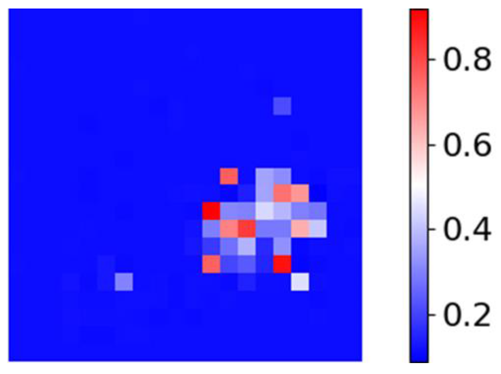
For example, from the dataset for the day 15 January: The dataset consists of date, location longitude, location dimension y and type of event. We imagine Zhengzhou city as a plane as shown below and map each area of Zhengzhou city to a 20 × 20 map according to its latitude and longitude. Through the steps of constructing the feature map, the feature map of violation cases in Zhengzhou City can be obtained, as shown in Figure 2.

3.2. Architecture of the Neural Network

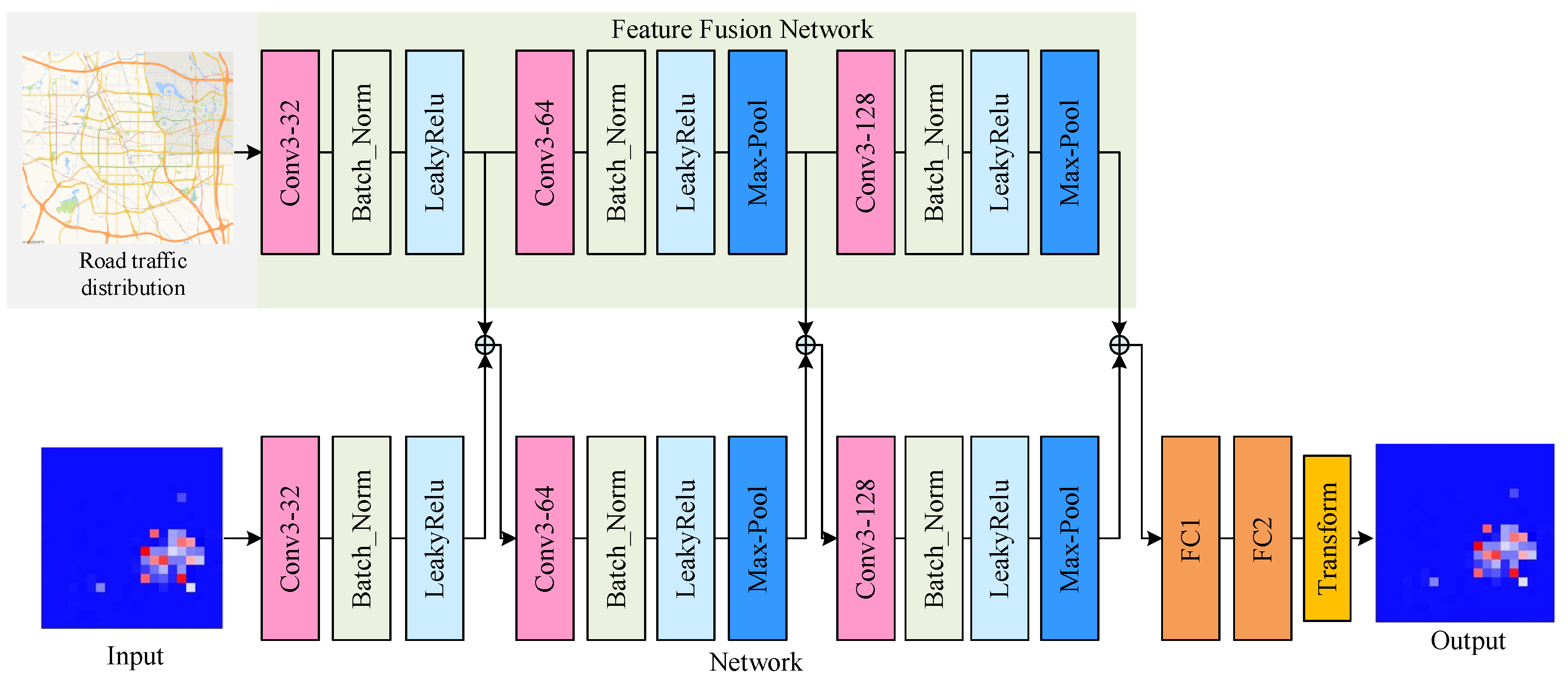
The prediction model proposed in this paper first uses a CNN for prediction, and the optimal depth of the convolutional layers is sought. Then, multiscale extraction feature fusion is achieved by using road network images as fusion features and extracting different scale features of the road network through multiscale convolution. The architecture graph of the neural network is shown in Figure 3. The specific details are presented in the convolutional neural network and feature fusion network below.

3.3. CNN

A class of neural networks that contain convolutional computations and have a deep structure. It was proposed by the mechanism of biological perceptual wilderness and is specifically designed to process neural networks with lattice-like structured data [44,45,46].

The overall architecture of CNN has four parts in total: an input layer, convolutional layer, pooling layer, and fully connected layer [47,48]. The CNN implements image processing as follows: the input layer reads in an image that has uniform size, and each neuron in each layer takes as input a set of small local nearest neighbors of the previous layer. The feature maps are then obtained by convolution operations, and at each position, the units from different feature maps obtain their own different types of features [49,50]. The convolutional layer is followed by a pooling layer connected to perform a reduced sampling operation [51,52]. The alternating distribution of convolution and pooling layers results in a progressive increase in the number of feature maps and a gradual decrease in resolution [53,54].

Each output mapping can combine the convolution with multiple input mappings [55].

$$X_j^l=f\left(\sum _{i\in M_j}{X}_i^{l-1}\times b_j^l\right)$$

(4)

where $M_j$ denotes the set of selected input mappings, the input mapping is i, the output feature is j and the output feature mapping is k, the convolution layer is l, and the additional bias is b.

The subsampling layer produces a downsampled version of the input map.

$$X_j^l=f\left({\beta }_j^{l}down\left(X_j^{l-1}\right)+b_j^l\right)$$

(5)

where down ( ) denotes a subsampling function, the multiplicative deviation is β, and the additive deviation is b.

The network selects which input maps to compute to obtain the output map j.

$$X_j^l=f\left(\sum _{i=1}^{N_{in}}{\alpha }_{ij}\left(X_i^{l-1}\times \right)+b_j^l\right)$$

(6)

Constraints need to be satisfied.

$$\sum _i{\alpha }_{ij}=1$$

(7)

$$0\le {\alpha }_{ij}\le 1$$

(8)

where ${\alpha }_{ij}$ denotes the weight of input mapping i given in forming output mapping j.

In this paper, a CNN is used as the main prediction network and the structure of the CNN is optimized by the depth of the convolutional layers. A multiscale feature extraction method is used to mine the information of urban road network, and the extracted information at different scales is fused. The fused information is finally used to predict the distribution of urban spatiotemporal events.

3.4. FFN

In this paper, a feature fusion network is proposed to integrate road network features with spatiotemporal event information through the following steps:

The first step is to process the road network image features, setting the image pixel size to be the same as the main network input feature image pixel size.

The second step is to construct a road network feature extraction model with the same convolutional layer structure as the main prediction model.

The third step is to fuse the different scales of road network information extracted by the fusion feature model into the main prediction model.

In the fourth step, the output of the first convolutional layer of the feature fusion model and the output of the first convolutional layer of the main prediction model are directly summed for feature fusion to obtain the fused features.

The fifth step is the road network feature extraction model. The first layer convolution output is used as its second layer convolution input for deep extraction of road network features. The second layer of convolutional input to the main prediction model is the features fused in step 4, using this convolutional layer for deep mining of features fused with road information.

The sixth step is to fuse the output of the second convolutional layer of the road feature extraction model with the output of the second convolutional layer of the main prediction model and use the fused features as the input of the third convolutional layer of the main prediction model.

In the seventh step, the input of the fully connected layer of the main prediction model is the fusion of the output of the convolution of the third layer of the road feature extraction model and the output of the convolution of the third layer of the main prediction model. The two fully connected layers are used to reduce the dimensionality of the data, and finally the one-dimensional output is converted to a two-dimensional distribution through dimensional transformation to achieve the prediction of the spatial crime distribution in the city at the next moment.

4. Case Study

4.1. Source of the Experimental Data

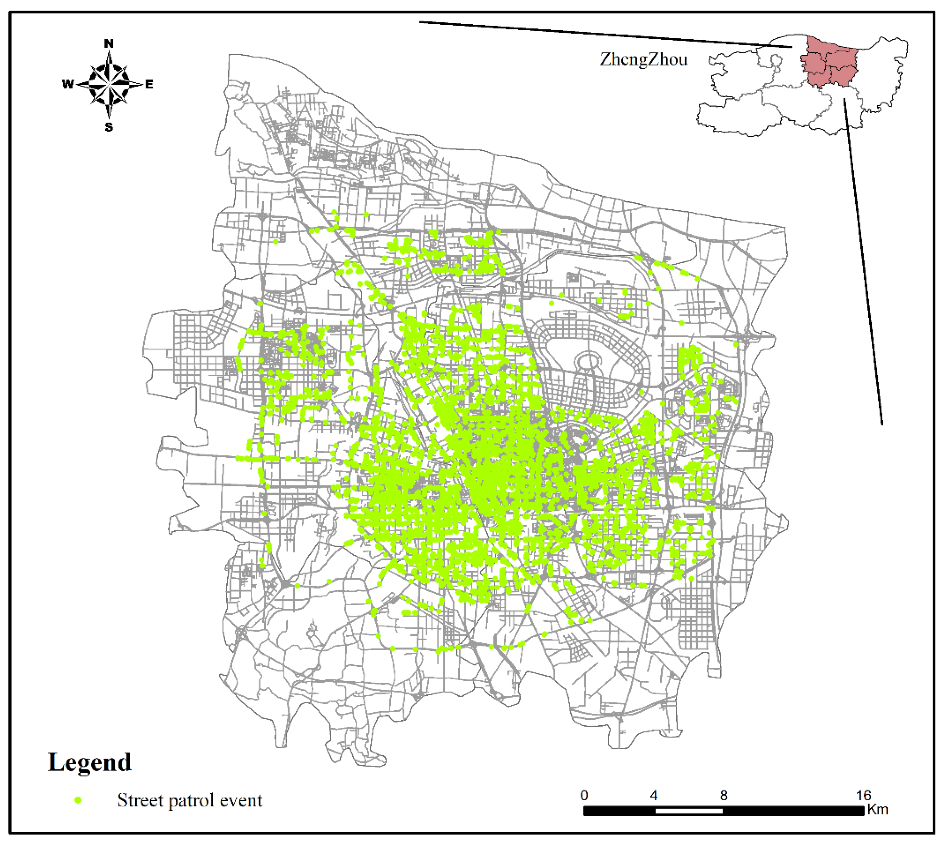
The coverage area of the urban patrol system in Zhengzhou City was used as the study area. The coverage area is currently approximately 567 km², including the five administrative districts within the East 4th Ring Road, South 4th Ring Road, West 4th Ring Road, and the 4th Ring Road surrounded by Dahe Road, as well as the aviation port economic comprehensive experimental zone. Within the study area, the street patrol data in Zhengzhou City were analyzed in conjunction with the 2018 road network data for the urban area, with datasets including specific dates, location longitude x, and location dimension y. The road network of Zhengzhou is illustrated in Figure 4, and sample data attribute information is shown in

Table 2. Attribute information of data.

Object-ID	Time	Coordinate_x	Coordinate_y
1	17 December 2018	482,484.9	3,801,871
2	28 December 2018	482,564.4	3,803,236
3	17 November 2018	482,561.8	3,803,244
4	6 November 2018	482,562.4	3,803,248
5	6 December 2018	482,565.2	3,803,429
6	14 November 2018	482,562.6	3,803,430
7	12 November 2018	482,579.4	3,803,439
8	10 December 2018	482,575.2	3,803,517
9	1 November 2018	482,608.4	3,803,613
10	21 December 2018	482,613.3	3,803,657

below.

This study is an analysis of a single day of patrol events. For example, there are 6098 street patrols records on 15 January 2018. The street patrol events are mainly in old urban areas like Erqi District and Guancheng District. The street patrol data are visualized on a map, as shown in Figure 5 below.

4.2. Experimental Details

Our model, called CNN-rFFN, was trained using the AdamW optimizer, with the batch size set to 30 and the number of iterations set to 1000. We applied the technique of exponentially decaying the learning rate with an initial learning rate of 0.0001. The specific network structure parameters for CNN-rFFN are shown in

Table 3. Network structure parameters for CNN-rFFN.

Name	Detail
CNN layer 1	input_size = 3, hidden_size = 32, kernel_size = 3, stride = 1, padding = 1, dropout = 0.5.
CNN layer 2	input_size = 32, hidden_size = 64, kernel_size = 3, stride = 1, padding = 1, dropout = 0.5, maxpool.
CNN layer 3	input_size = 64, hidden_size = 128, kernel_size = 5, stride = 1, padding = 1, dropout = 0.5, maxpool.
Feature fusion CNN layer 1	input_size = 3, hidden_size = 32, kernel_size = 3, stride = 1, padding = 1, dropout = 0.5.
Feature fusion CNN layer 2	input_size = 32, hidden_size = 64, kernel_size = 3, stride = 1, padding = 1, dropout = 0.5, maxpool.
Feature fusion CNN layer 3	input_size = 64, hidden_size = 128, kernel_size = 5, stride = 1, padding = 1, dropout = 0.5, maxpool.
Full connected layer (FC3)	in_features = 9 × 9 × 128, out_features = 64 × 64
Full connected layer (FC3)	in_features = 64 × 64, out_features = 40 × 40
Output layer(out)	out_features = 40 × 40
Batch_size	30
Optimiser	AdamW
Loss function	Huberloss
Activation function	LeakyRelu
Epochs	1000
Learning rate	0.001

below.

4.3. Result Analysis

We evaluate the effectiveness of the proposed algorithms in this section. The prediction performance of each algorithm is measured using four metrics, namely, the root mean square error (RMSE), the mean absolute error (MAE), the mean absolute percentage error (MAPE), and the R-squared (R²). The definitions are as follows:

$$RMSE={\displaystyle }{\left({\displaystyle \frac{1}{n}}{\sum }_{i=1}^n{\left(X_{t+T}-{\widehat{X}}_{t+T}\right)}^2\right)}^{{\displaystyle \frac{1}{2}}}$$

(9)

$$MAE=\left({\displaystyle \frac{1}{n}}{\sum }_{i=1}^n\left|X_{t+T}-{\widehat{X}}_{t+T}\right|\right)$$

(10)

$$MAPE={\displaystyle \frac{1}{n}}{\sum }_{i=1}^n{\displaystyle \frac{\left|X_{t+T}-{\widehat{X}}_{t+T}\right|}{\left|X_{t+T}\right|}}$$

(11)

$$R^2=1-{\displaystyle \frac{{\sum }_{i=1}^n{\left(X_{t+T}-{\widehat{X}}_{t+T}\right)}^2}{{\sum }_{i=1}^n{\left({\overline{X}}_{t+T}-{\widehat{X}}_{t+T}\right)}^2}}$$

(12)

For the three metrics RMSE, MAE, and MAPE, the lower the value is, the better the model performance. For the metric $R^2$, the higher the value is, the better the model fits [56,57].

4.4. Finding the Optimal Number of CNN Layers

The convolutional neural network used in this method requires optimization of the number of convolutional layers. The feature dimension is set to 20*20, and the convolutional layers are divided into one-layer convolution, two-layer convolution, three-layer convolution, and four-layer convolution. The test was repeated for different numbers of layers, and the average RMSE, MAE, and MAPE of the test set were calculated as the evaluation metric. The table of evaluation metrics for the number of convolutional layers of the predicted event distribution is shown in

Table 4. Convolutional layer evaluation metrics.

Layer	MAPE	MAE	RMSE	R2
1	0.0557	0.0099	0.0407	0.7910
2	0.0642	0.0111	0.0396	0.6610
3	0.0274	0.0061	0.0376	0.9131
4	0.0320	0.0068	0.0380	0.8437

. The optimal number of convolution layers is determined to be three layers based on the metrics in the table.

In order to discover the optimal number of layers of the convolutional neural network more visually, randomly selected times from the dataset are used to validate the predictive performance of the model. In order to increase the credibility of the visualization performance, two sets of time visualizations are provided, as shown in Figure 6.

Each subplot in Figure 5 has two subplots, from top to bottom, of ground truth and predicted results. Observation of Figure 5 reveals that the colors in the heat map of predicted cases are darker than the true values when the number of convolution layers are one, two, and four. This indicates that the predicted number of cases is more than the true number of cases in this region and there is an error with the true distribution. The event prediction accuracy is highest when the number of convolution layers is three.

4.5. Finding the Optimal Number of Size of Feature Map

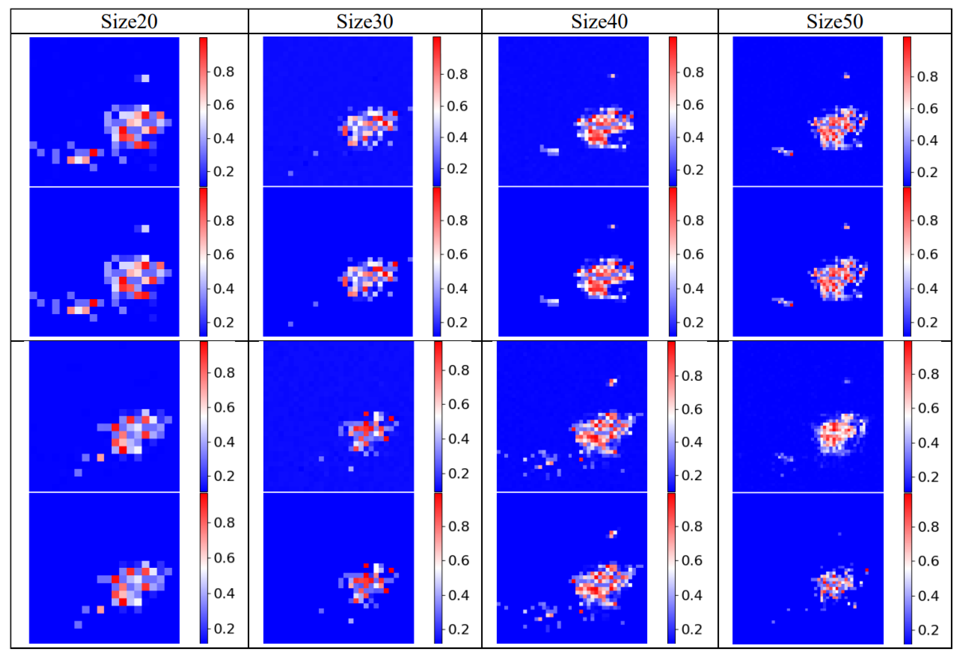
This method requires optimization of the size of the constructed feature map, which is divided into 20 × 20, 30 × 30, 40 × 40, and 50 × 50 squares. We tested this iteratively by using different feature map sizes. The averages of the RMSE, MAE, and MAPE of the test set are calculated as evaluation metrics to determine the optimal feature map size. The table of evaluation indicators for the size of the feature map of the predicted event distribution is shown in

Table 5. Evaluation metrics for feature map size.

Size	MAPE	MAE	RMSE	R2
20	0.0303	0.0069	0.0385	0.8848
30	0.0436	0.0092	0.0388	0.7772
40	0.0379	0.0072	0.0348	0.9036
50	0.0434	0.0079	0.0374	0.8279

, and analysis of the table values shows that the feature map size is optimal at 40 × 40.

In order to discover the optimal feature map size more intuitively, randomly selected times from the dataset are used to show the predictive performance of the model. To increase the confidence in the visualization performance, two sets of time visualizations are provided, as shown in Figure 7. In each subfigure, the ground truth and prediction results are shown in order from top to bottom. Observation of the visualized image reveals that the event prediction accuracy is highest when the feature map is 40 × 40.

5. Discussions

5.1. Impact of the Time Factor

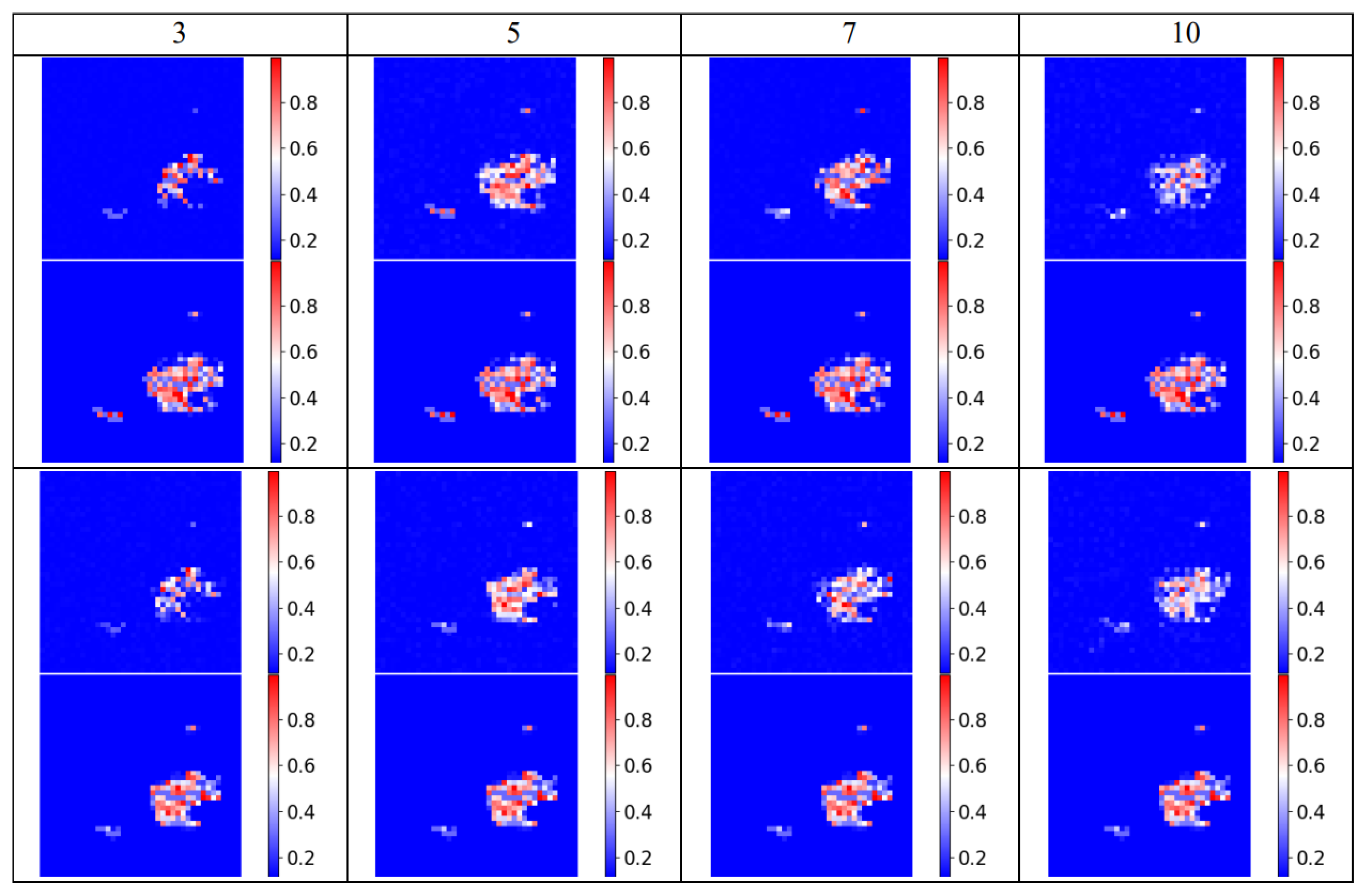
There is a correlation between street patrol incidents on the same day and incidents that occurred at that location in the past. This can affect the probability of a violation case occurring. Therefore, patrol incidents that have occurred at a given time within the location are counted and constructed to include temporal attribute features. Statistics are kept on cases that occurred in a fixed area 3 days, 5 days, 7 days, and 10 days prior to the occurrence of the event. The results obtained are shown in

Table 6. Predictors of tectonic features for different time periods.

Size	MAPE	MAE	RMSE	R2
3	0.0679	0.0231	0.0582	0.000237
5	0.0557	0.0181	0.0348	0.000319
7	0.0780	0.0276	0.1145	0.000276
10	0.0912	0.0219	0.0799	0.000102

below.

To discover the optimal feature map size more intuitively, we randomly selected times from the dataset to show the predictive performance of the model. To increase confidence in the visualized performance, we provide visualizations for two sets of times, as shown in Figure 8.

In each subplot, the ground truth and predicted results are shown in order from top to bottom. Observing the visualized images and combining them with the algorithm evaluation metrics table, it is found that the prediction accuracy is highest when the time length is 5.

5.2. Comparison with Other Algorithms

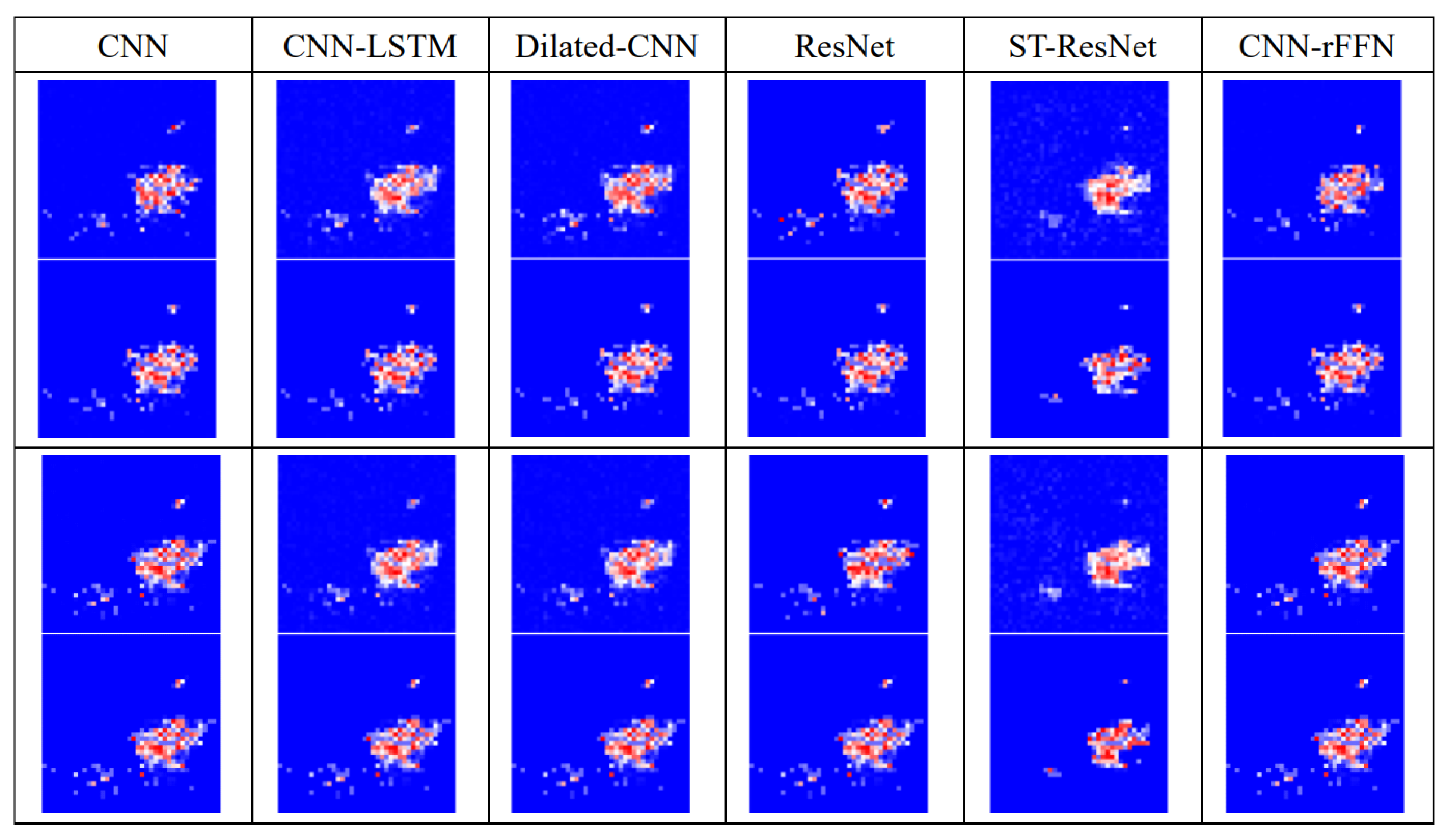
To validate the performance of our model, and to ensure the stability and prediction accuracy, we compared four algorithms with the algorithms in this paper, including CNN, CNN-LSTM, Dilated-CNN, and ResNet [58,59,60,61].

The experiments were tested iteratively, and the mean values of MAPE, MAE, and RMSE were selected for comparative analysis. The table of evaluation metrics for different algorithms is shown in

Table 7. Evaluation metrics for different algorithms.

Model	MAPE	MAE	RMSE	R2
CNN	0.0440	0.0083	0.0383	0.9105
CNN-LSTM	0.0672	0.0159	0.0598	0.8689
Dilated-CNN	0.0291	0.0059	0.0376	0.9174
ResNet	0.0273	00061	0.0375	0.9120
ST-ResNet	0.0270	0.0237	0.0380	0.7710
CNN-rFFN	0.0265	0.0058	0.0375	0.9430

. The results show that the algorithm in this paper has the lowest error, the highest accuracy, and the highest stability.

In order to reveal the effectiveness of the model more intuitively, two time gaps were randomly selected from the dataset to show the prediction performance of the model in this paper, as shown in Figure 9 below. In each subfigure, the ground truth and prediction results are shown in order from top to bottom. The area circled from the circle in the figure marks the error that exists between the prediction result and the true value. Observation of the following images reveals that the proposed model achieves a high degree of prediction of urban spatiotemporal events.

5.3. Parameter Sensitivity Analysis

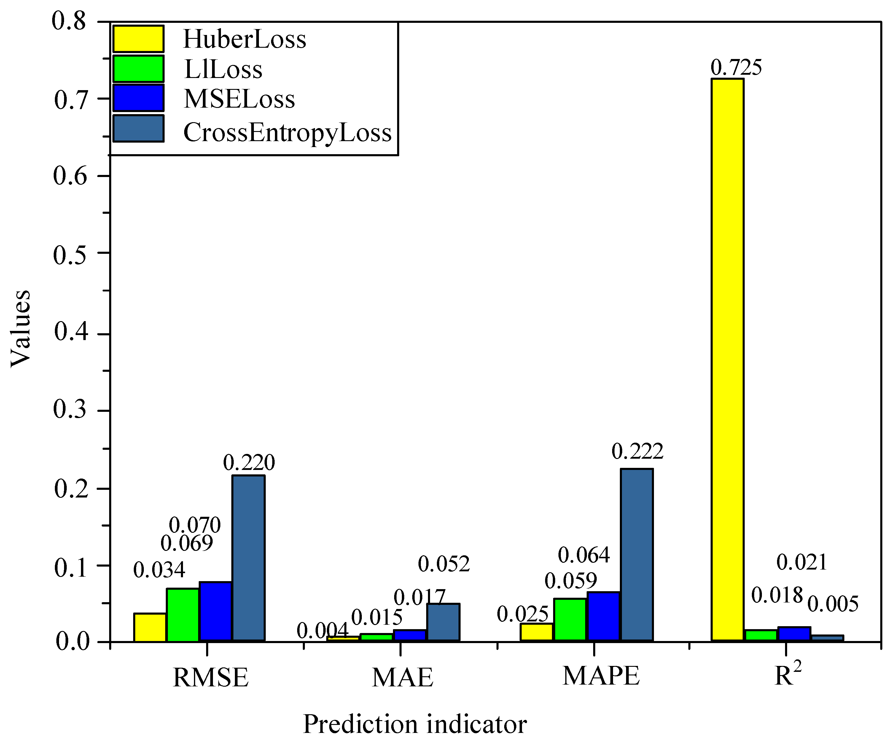
To further demonstrate the effectiveness of our proposed method, experiments were conducted by setting different parameters, including the minimum number of iteration batches, the learning rate, the activation function, and the loss function. We randomly selected 70% of the data to train the model and then validated the model using data from October 2018 and analyzed the sensitivity of the model based on the predictive evaluation metrics obtained from the validation results.

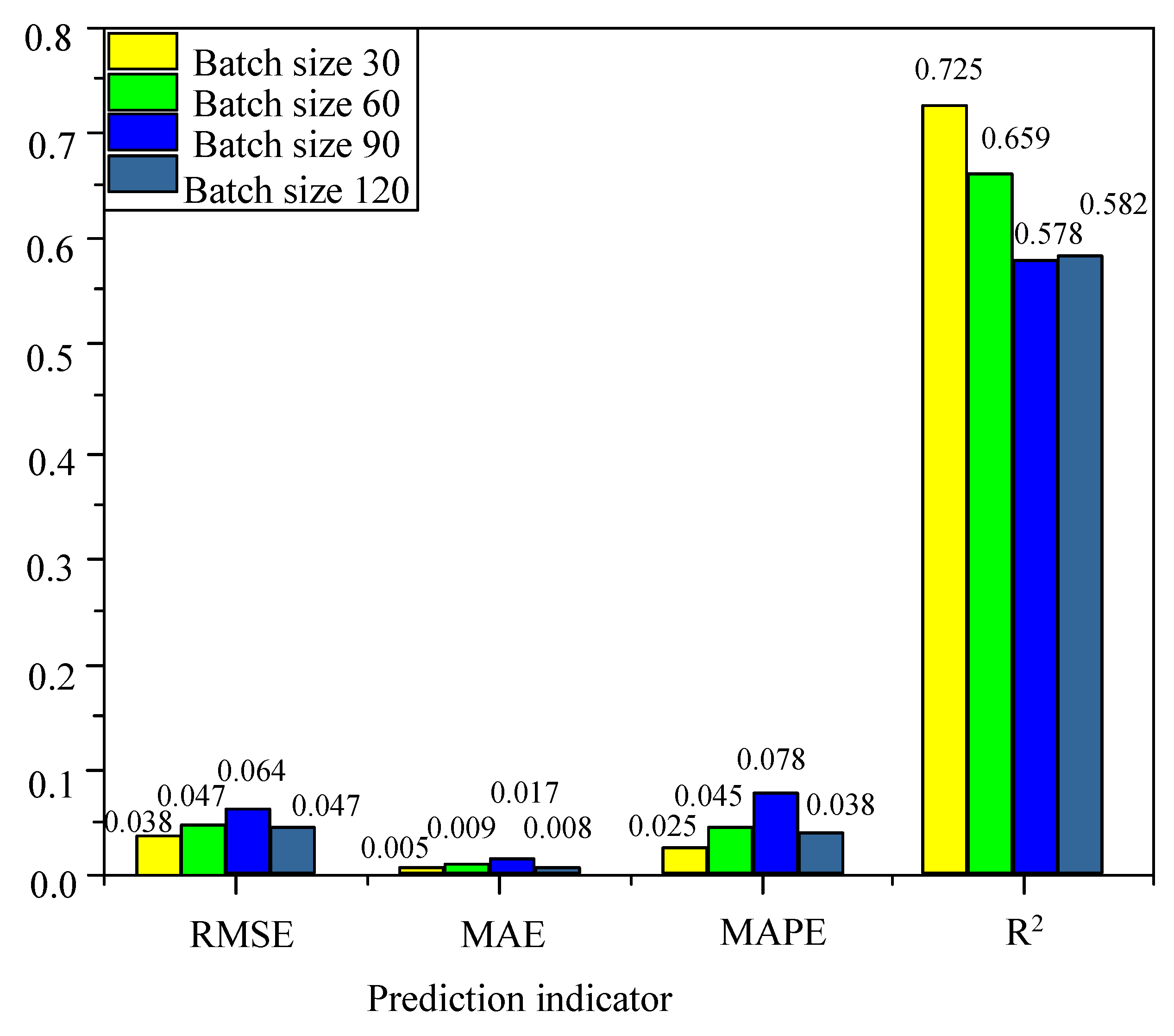
First, a sensitivity analysis of the minimum iteration batch size of the model was carried out, and the results are shown in Figure 10 below. Batching with all the data can cause the model to fall into a local optimum. By dividing the overall sample into smaller samples, mini-batches reduce the likelihood of the model falling into a local optimum. They also allocate computing resources rationally, preventing the computer from running out of memory due to excessive data [62]. The predictor of this bar chart shows the reasonableness of the minimum number of iterations chosen in this paper. From the figure, the minimum number of iterations is 30 with minimum values of RMSE, MAE, and MAPE and maximum value of R². It shows that the best results are obtained when the minimum number of iterations is chosen to be 30.

Second, the model learning rate sensitivity was analyzed, as shown in Figure 11 below. The learning rate determines the learning step size of the model. When the learning rate is too large, the model will not converge, and when the learning rate is small, the model will converge too slowly [63]. The indicator values in the graph are best when the learning rate is 0.001. The predictive indicators of this bar chart illustrate that the best value was obtained in this paper when a learning rate of 0.001 was selected.

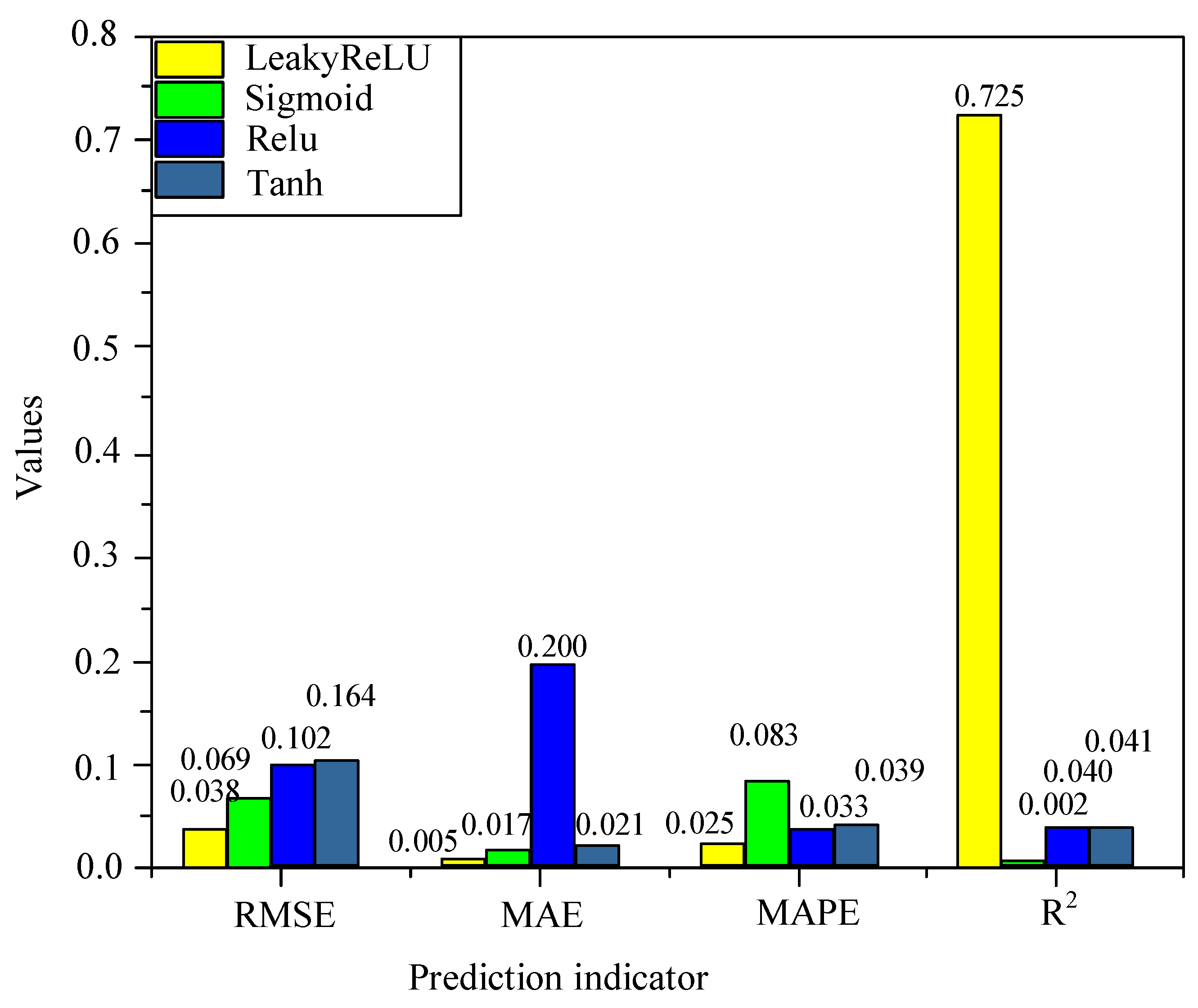
Then, the model activation function sensitivity was analyzed, as shown in Figure 12 below. The activation function determines the nonlinear relationship between the input and output of a neural network. It determines whether the neuron receives information subject to retention or not. Commonly used activation functions include the sigmoid, ReLU, tanh, and the ReLU function variant LeakyReLU [64]. Observing this figure, it can be concluded that the LeakyReLU function handles the problem of the zero gradient of negative inputs by giving them a very small linear component. The model neuron information retention problem is improved, and the prediction accuracy of the model is enhanced. According to the description of the prediction metrics, the best prediction is achieved when using the LeakyReLU function.

Finally, a sensitivity analysis of the model loss function was carried out, and the results are shown in Figure 13 below. The core of a neural network is to minimize the loss function by continuously adjusting the network parameters. The loss function is used to define the error between the predicted and true values of the training samples; the smaller the value is, the better the prediction performance of the training model. Commonly used loss functions include Crossentroloss, MSEloss, L1loss, and Huberloss [65]. The analysis of the graph shows that model obtained much better predictions using Huberloss than the other loss functions. Huberloss is a loss function combining MSE and MAE; the MSE is used when the error is close to zero, and the MAE is used when the error is large. This variation increases the robustness of the training. According to the predictors in the figure, it shows that the best value can be obtained when the loss function is chosen as Huberloss.

The results of the four model parameters—minimum iteration batch size, learning rate, activation function, and loss function—combine to reflect that the prediction performance of the model is very sensitive to the gradient descent problem of the training process. The purpose of setting different parameters is to find the lowest point of the loss function. When the parameters are not set properly, the model will fall into a local optimum, resulting in poor prediction performance of the final trained model. The above analysis justifies the setting of the minimum number of iterative batches, learning rate, activation function, and loss function in this paper. After several experimental validations, the learning rate was chosen to be 0.001, the activation function was chosen to be LeakyReLU, the loss function was chosen to be Huberloss, and the minimum number of iterative batches was 30.

5.4. Ablation Experiment

Our proposed multiscale feature fusion model consists of three layers of convolutional networks. The feature extraction process is refined progressively, resulting in distinct features being extracted from different layers. Consequently, this model effectively fuses features of varying scales from these diverse layers. To illustrate the impact of various scale features on predictive performance, we developed a feature fusion model incorporating a single layer of convolution. The output from this convolutional layer was integrated into the main network, designated as Ablation Trial 1. Additionally, we constructed another feature fusion model utilizing two layers of convolution, where the output features from the entire model were fused with the main network; this is referred to as Ablation Trial 2. A three-layer convolution is used to form a feature fusion model that fuses the output features of the last layer of convolution to the main network, which is labelled as Ablation Trial 3. A two-layer convolution is used to form the feature fusion model, and the output features of the first layer convolution and the second layer convolution are fused to the main network, respectively, which is labelled as Ablation Trial 4.

The four models mentioned above and the proposed method constitute the ablation test. The models are trained using the same data and the superiority of the proposed method is verified based on the predictors of the validation set. The prediction results of the feature fusion models with different scales randomly selected are shown in

Table 8. Results of ablation experiment.

Model	MAPE	MAE	RMSE
Fusion 1	0.0732	0.0192	0.0939
Fusion 2	0.0680	0.0185	0.0592
Fusion 3	0.0807	0.0187	0.0739
Fusion 4	0.0500	0.0107	0.0528
CNN-rFFN	0.0416	0.0091	0.0447

.

According to the comparison graph of predictions and the associated prediction indices, it is evident that when employing single-scale feature fusion, varying depths of fused feature extraction yield different impacts on the prediction model. Furthermore, the performance of the prediction model improves as the scale of feature fusion increases. The predictive performance of the multiscale feature fusion model is higher than that of the single-scale feature fusion model, and the results show that the proposed multiscale feature fusion can effectively improve the predictive performance of the model.

6. Conclusions

The important cycle of smart cities lies in the prediction of spatiotemporal dynamic events in urban areas. This is of great importance for protecting the safety of inhabitants and maintaining the sustainability of the city. This paper proposes a method for urban spatiotemporal event prediction based on CNN and feature fusion network. First, predictions are made by feature map construction and the CNN, and the optimal feature map size and number of convolutional layers are selected. Then, the information on the urban road network is extracted using multiscale convolution, and the extracted road network features are incorporated into the CNN. This method improves the predictive performance of the algorithm by optimizing the CNN with a road feature fusion network. Experimental analysis of the method in this paper was carried out to find the optimal feature map and the number of convolutional layers. The method was also compared with several other methods, and the experimental results show that the urban spatiotemporal event prediction method in this paper has the highest accuracy.

In future work, we will continue to collect data for a number of years, expanding the data recording period. We also intend to test our model with other urban spatiotemporal event data to demonstrate its potential application in a wider range of areas. In addition, the predictive generalization capability of the model in this paper will be extended by incremental learning strategies to improve the applicability of the models built. Finally, a complete spatiotemporal event prediction system will be established through the prediction framework of this paper to accurately predict the occurrence of spatiotemporal events in urban areas through the collection of data.

References

1. Zheng, Y.; Capra, L.; Wolfson, O.; Yang, H. Urban computing: Concepts, methodologies, and applications. ACM Trans. Intell. Syst. Technol. TIST 2014, 5, 1–55. [Google Scholar] [CrossRef]
2. Kim, D.; Kim, S. Role and challenge of technology toward a smart sustainable city: Topic modeling, classification, and time series analysis using information and communication technology patent data. Sustain. Cities Soc. 2022, 82, 103888. [Google Scholar] [CrossRef]
3. Catlett, C.; Cesario, E.; Talia, D.; Vinci, A. Spatiotemporal crime predictions in smart cities: A data-driven approach and experiments. Pervasive Mob. Comput. 2019, 53, 62–74. [Google Scholar] [CrossRef]
4. Okawa, M.; Iwata, T.; Kurashima, T.; Tanaka, Y.; Toda, H.; Ueda, N. Deep mixture point processes: Spatiotemporal event prediction with rich contextual information. In Proceedings of the 25th ACM SIGKDD International Conference on Knowledge Discovery & Data Mining, Anchorage, AK, USA, 4–8 August 2019; pp. 373–383. [Google Scholar] [CrossRef]
5. Butt, U.M.; Letchmunan, S.; Hassan, F.H.; Ali, M.; Baqir, A.; Sherazi, H.H.R. Spatiotemporal crime hotspot detection and prediction: A systematic literature review. IEEE Access 2020, 8, 166553–166574. [Google Scholar] [CrossRef]
6. Jin, G.; Liu, C.; Xi, Z.; Sha, H.; Liu, Y.; Huang, J. Adaptive Dual-View WaveNet for urban spatio–temporal event prediction. Inf. Sci. 2022, 588, 315–330. [Google Scholar] [CrossRef]
7. Zhang, Y.; Cheng, T. Graph deep learning model for network-based predictive hotspot mapping of sparse spatiotemporal events. Comput. Environ. Urban Syst. 2020, 79, 101403. [Google Scholar] [CrossRef]
8. Shen, B.; Liang, X.; Ouyang, Y.; Liu, M.; Zheng, W.; Carley, K.M. Stepdeep: A novel spatiotemporal mobility event prediction framework based on deep neural network. In Proceedings of the 24th ACM SIGKDD International Conference on Knowledge Discovery & Data Mining, London, UK, 19–23 August 2018; pp. 724–733. [Google Scholar] [CrossRef]
9. Yu, M.; Bambacus, M.; Cervone, G.; Clarke, K.; Duffy, D.; Huang, Q.; Li, J.; Li, W.; Li, Z.; Liu, Q.; et al. Spatiotemporal event detection: A review. Int. J. Digit. Earth 2020, 13, 1339–1365. [Google Scholar] [CrossRef]
10. Fox, J.; Brown, D.E. Using temporal indicator functions with generalized linear models for spatiotemporal event prediction. Procedia Comput. Sci. 2012, 8, 106–111. [Google Scholar] [CrossRef]
11. Chen, L.; Zhang, D.; Wang, L.; Yang, D.; Ma, X.; Li, S.; Wu, Z.; Pan, G.; Nguyen, T.M.T.; Jakubowicz, J. Dynamic cluster-based over-demand prediction in bike sharing systems. In Proceedings of the 18th Ubicomp, ACM, Singapore, 8–12 October 2016; pp. 841–852. [Google Scholar] [CrossRef]
12. Hoang, M.X.; Zheng, Y.; Singh, A.K. FCCF: Forecasting citywide crowd flows based on big data. In Proceedings of the 24th ACM SIGSPATIAL International Conference on Advances in Geographic Information Systems, San Francisco, CA, USA, 31 October 2016. [Google Scholar] [CrossRef]
13. Zhang, J.; Zheng, Y.; Qi, D.; Li, R.; Yi, X.; Li, T. Predicting citywide crowd flows using deep spatiotemporal residual networks. Artif. Intell. 2018, 259, 147–166. [Google Scholar] [CrossRef]
14. Wendland, H. Piecewise polynomial, positive definite and compactly supported radial functions of minimal degree. Adv. Comput. Math. 1995, 4, 389–396. [Google Scholar] [CrossRef]
15. Tian, C.; Chan, W.K. Spatio-temporal attention wavenet: A deep learning framework for traffic prediction considering spatio-temporal dependencies. IET Intell. Transp. Syst. 2021, 15, 549–561. [Google Scholar] [CrossRef]
16. Zhang, J.; Zheng, Y.; Sun, J.; Qi, D. Flow prediction in spatiotemporal networks based on multitask deep learning. IEEE Trans. Knowl. Data Eng. 2019, 32, 468–478. [Google Scholar] [CrossRef]
17. Zhang, W.; Yu, Y.; Qi, Y.; Shu, F.; Wang, Y. Short-term traffic flow prediction based on spatiotemporal analysis and CNN deep learning. Transp. A Transp. Sci. 2019, 15, 1688–1711. [Google Scholar] [CrossRef]
18. Cao, P.; Dai, F.; Liu, G.; Yang, J.; Huang, B. A survey of traffic prediction based on deep neural network: Data, methods and challenges. In Proceedings of the Cloud Computing: 11th EAI International Conference, CloudComp 2021, Virtual Event, 9–10 December 2021; Springer International Publishing: Cham, Switzerland, 2022; pp. 17–29. [Google Scholar] [CrossRef]
19. Yao, H.; Liu, Y.; Wei, Y.; Tang, X.; Li, Z. Learning from multiple cities: A meta-learning approach for spatiotemporal prediction. In Proceedings of the World Wide Web Conference, San Francisco, CA, USA, 13–17 May 2019; pp. 2181–2191. [Google Scholar] [CrossRef]
20. Kumar, S.V. Traffic flow prediction using Kalman filtering technique. Procedia Eng. 2017, 187, 582–587. [Google Scholar] [CrossRef]
21. Xu, L.; Chen, N.; Chen, Z.; Zhang, C.; Yu, H. Spatiotemporal forecasting in earth system science: Methods, uncertainties, predictability and future directions. Earth-Sci. Rev. 2021, 222, 103828. [Google Scholar] [CrossRef]
22. Guo, J.; Huang, W.; Williams, B.M. Adaptive Kalman filter approach for stochastic short-term traffic flow rate prediction and uncertainty quantification. Transp. Res. Part C Emerg. Technol. 2014, 43, 50–64. [Google Scholar] [CrossRef]
23. Kumar, S.V.; Vanajakshi, L. Short-term traffic flow prediction using seasonal ARIMA model with limited input data. Eur. Transp. Res. Rev. 2015, 7, 21. [Google Scholar] [CrossRef]
24. Chen, P.; Yuan, H.; Shu, X. Forecasting crime using the arima model. In Proceedings of the 2008 Fifth International Conference on Fuzzy Systems and Knowledge Discovery, Jinen, China, 18–20 October 2008; Volume 5, pp. 627–630. [Google Scholar] [CrossRef]
25. Chamlin, M.B. Crime and arrests: An autoregressive integrated moving average (ARIMA) approach. J. Quant. Criminol. 1988, 4, 247–258. [Google Scholar] [CrossRef]
26. Alghamdi, T.; Elgazzar, K.; Bayoumi, M.; Sharaf, T.; Shah, S. Forecasting traffic congestion using ARIMA modeling. In Proceedings of the 15th International Wireless Communications & Mobile Computing Conference (IWCMC), Tangier, Morocco, 24–28 June 2019; pp. 1227–1232. [Google Scholar] [CrossRef]
27. Okutani, I.; Stephanedes, Y.J. Dynamic prediction of traffic volume through Kalman filtering theory. Transp. Res. Part B Methodol. 1984, 18, 1–11. [Google Scholar] [CrossRef]
28. Lu, B.; Martin, C.; Fotheringhama, A.S. Geographically weighted regression using a non-Euclidean distance metric with a study on London house price data. Procedia Environ. Sci. 2011, 7, 92–97. [Google Scholar] [CrossRef]
29. Yao, S.; Wei, M.; Yan, L.; Wang, C.; Dong, X.; Liu, F.; Xiong, Y. Prediction of crime hotspots based on spatio factors of random forest. In Proceedings of the 15th International Conference on Computer Science & Education (ICCSE), Piscataway, NJ, USA, 18–22 August 2020; pp. 811–815. [Google Scholar] [CrossRef]
30. Cheng, R.; Zhang, M.; Yu, X. Prediction model for road traffic accident based on random forest. In Proceedings of the Education Science and Development of the International Conference (ICESD), Jakarta, Indonesia, 19–20 January 2019; pp. 12–13. [Google Scholar]
31. Nasridinov, A.; Ihm, S.Y.; Park, Y.H. A decision tree-based classification model for crime prediction. In Information Technology Convergence; Springer: Dordrecht, The Netherlands, 2013; pp. 531–538. [Google Scholar] [CrossRef]
32. Hassani, H.; Huang, X.; Silva, E.S.; Ghodsi, M. A review of data mining applications in crime. Stat. Anal. Data Min. ASA Data Sci. J. 2016, 9, 139–154. [Google Scholar] [CrossRef]
33. Kim, S.; Joshi, P.; Kalsi, P.S.; Taheri, P. Crime analysis through machine learning. In Proceedings of the 2 IEEE 9th Annual Information Technology, Electronics and Mobile Communication Conference (IEMCON), Vancouver, BC, Canada, 1–3 November 2018; pp. 415–420. [Google Scholar] [CrossRef]
34. Khan, M.; Ali, A.; Alharbi, Y. Predicting and Preventing Crime: A Crime Prediction Model Using San Francisco Crime Data by Classification Techniques. Complexity 2022, 2022, 4830411. [Google Scholar] [CrossRef]
35. Jiang, W.; Luo, J.; He, M.; Gu, W. Graph neural network for traffic forecasting: The research progress. ISPRS Int. J. Geo-Inf. 2023, 12, 100. [Google Scholar] [CrossRef]
36. Geng, Z.; Xu, J.; Wu, R.; Zhao, C.; Wang, J.; Li, Y.; Zhang, C. STGAFormer: Spatial–temporal Gated Attention Transformer based Graph Neural Network for traffic flow forecasting. Inf. Fusion 2024, 105, 102228. [Google Scholar] [CrossRef]
37. Chen, J.; Zheng, L.; Hu, Y.; Wang, W.; Zhang, H.; Hu, X. Traffic flow matrix-based graph neural network with attention mechanism for traffic flow prediction. Inf. Fusion 2024, 104, 102146. [Google Scholar] [CrossRef]
38. Ilhan, F.; Tekin, S.F.; Aksoy, B. Spatiotemporal Crime Prediction with Temporally Hierarchical Convolutional Neural Networks. In Proceedings of the 28th Signal Processing and Communications Applications Conference (SIU), Gaziantep, Turkey, 5–7 October 2020; pp. 1–4. [Google Scholar] [CrossRef]
39. Xiao, Y.; Wang, X.; Feng, W.; Tian, H.; Wu, S.; Li, L. Predicting crime locations based on long short term memory and convolutional neural networks. Data Anal. Knowl. Discov. 2018, 2, 15–20. [Google Scholar]
40. Haque, M.R.; Hafiz, R.; Al Azad, A.; Adnan, Y.; Mishu, S.A.; Khatun, A.; Uddin, M.S. Crime detection and criminal recognition to intervene in interpersonal violence using deep convolutional neural network with transfer learning. Int. J. Ambient Comput. Intell. IJACI 2021, 12, 1–14. [Google Scholar] [CrossRef]
41. Andersson, V.O.; Birck MA, F.; Araujo, R.M. Investigating crime rate prediction using street-level images and siamese convolutional neural networks. In Proceedings of the Latin American Workshop on Computational Neuroscience, Porto Alegre, Brazil, 22–24 November 2017; Springer: Cham, Switzerland, 2017; pp. 81–93. [Google Scholar] [CrossRef]
42. Andersson, V.O.; Birck, M.A.; Araújo, R.M.; Cechinel, C. Towards crime rate prediction through street-level images and siamese convolutional neural networks. ENIAC-Encontro Nac. Inteligência Artif. E Comput. 2017, 14, 448–458. Available online: https://www.researchgate.net/publication/321779586_Towards_Crime_Rate_Prediction_through_Street-level_Images_and_Siamese_Convolutional_Neural_Networks (accessed on 19 September 2024).
43. Miao, J.; Yang, T.; Sun, L.; Fei, X.; Niu, L.; Shi, Y. Graph regularized locally linear embedding for unsupervised feature selection. Pattern Recognit. 2022, 122, 108299. [Google Scholar] [CrossRef]
44. Li, Y.; Hao, Z.; Lei, H. Survey of convolutional neural network. J. Comput. Appl. 2016, 36, 2508. [Google Scholar]
45. Li, Z.; Liu, F.; Yang, W.; Peng, S.; Zhou, J. A survey of convolutional neural networks: Analysis, applications, and prospects. IEEE Trans. Neural Netw. Learn. Syst. 2021, 33, 6999–7019. [Google Scholar] [CrossRef] [PubMed]
46. Khan, A.; Sohail, A.; Zahoora, U.; Qureshi, A.S. A survey of the recent architectures of deep convolutional neural networks. Artif. Intell. Rev. 2020, 53, 5455–5516. [Google Scholar] [CrossRef]
47. Sakib, S.; Ahmed, N.; Kabir, A.J.; Ahmed, H. An overview of convolutional neural network: Its architecture and applications. Preprints 2019. [Google Scholar] [CrossRef]
48. Ghosh, A.; Sufian, A.; Sultana, F.; Chakrabarti, A.; De, D. Fundamental concepts of convolutional neural network. In Recent Trends and Advances in Artificial Intelligence and Internet of Things; Springer: Cham, Switzerland, 2020; pp. 519–567. [Google Scholar] [CrossRef]
49. Aloysius, N.; Geetha, M. A review on deep convolutional neural networks. In Proceedings of the International Conference on Communication and Signal Processing (ICCSP), Melmaruvathur, India, 6–8 April 2017; pp. 588–592. [Google Scholar] [CrossRef]
50. Liu, M.; Shi, J.; Li, Z.; Li, C.; Zhu, J.; Liu, S. Towards better analysis of deep convolutional neural networks. IEEE Trans. Vis. Comput. Graph. 2016, 23, 91–100. [Google Scholar] [CrossRef] [PubMed]
51. Zhang, Q.; Zhang, M.; Chen, T.; Sun, Z.; Ma, Y.; Yu, B. Recent advances in convolutional neural network acceleration. Neurocomputing 2019, 323, 37–51. [Google Scholar] [CrossRef]
52. Dhillon, A.; Verma, G.K. Convolutional neural network: A review of models, methodologies and applications to object detection. Prog. Artif. Intell. 2020, 9, 85–112. [Google Scholar] [CrossRef]
53. Porzi, L.; Rota Bulò, S.; Lepri, B.; Ricci, E. Predicting and understanding urban perception with convolutional neural networks. In Proceedings of the 23rd ACM International Conference on Multimedia, Brisbane, Australia, 13 October 2015; pp. 139–148. [Google Scholar] [CrossRef]
54. Bouvrie, J. Notes on Convolutional Neural Network. 2006. Available online: http://web.mit.edu/jvb/www/papers/cnn_tutorial.pdf (accessed on 19 September 2024).
55. Zhang, Q. Convolutional neural networks. In Proceedings of the 3rd International Conference on Electromechanical Control Technology and Transportation, Chongqing, China, 19–21 January 2018; pp. 434–439. [Google Scholar]
56. Varshini, A.G.P.; Kumari, K.A.; Janani, D.; Soundariya, S. Comparative analysis of Machine learning and Deep learning algorithms for Software Effort Estimation. J. Phys. Conf. Series 2021, 1767, 012019. [Google Scholar] [CrossRef]
57. Aptula, A.O.; Jeliazkova, N.G.; Schultz, T.W.; Cronin, M.T.D. The better predictive model: High q2 for the training set or low root mean square error of prediction for the test set. QSAR Comb. Sci. 2005, 24, 385–396. [Google Scholar] [CrossRef]
58. Alzubaidi, L.; Zhang, J.; Humaidi, A.J.; Al-Dujaili, A.; Duan, Y.; Al-Shamma, O.; Santamaria, J.; Fadhel, M.A.; Al-Amidie, M.; Farhan, L. Review of deep learning: Concepts, CNN architectures, challenges, applications, future directions. J. Big Data 2021, 8, 1–74. [Google Scholar] [CrossRef]
59. Rostamian, A.; O’Hara, J.G. Event prediction within directional change framework using a CNN-LSTM model. Neural Comput. Appl. 2022, 34, 17193–17205. [Google Scholar] [CrossRef]
60. Borovykh, A.; Bohte, S.; Oosterlee, C.W. Dilated convolutional neural networks for time series forecasting. J. Comput. Financ. Forthcom. 2018. [Google Scholar] [CrossRef]
61. Wu, Z.; Shen, C.; Van Den Hengel, A. Wider or deeper: Revisiting the resnet model for visual recognition. Pattern Recognit. 2019, 90, 119–133. [Google Scholar] [CrossRef]
62. Radiuk, P.M. Impact of training set batch size on the performance of convolutional neural networks for diverse datasets. Inf. Technol. Manag. Sci. 2017, 20, 20–24. Available online: https://itms-journals.rtu.lv/article/view/itms-2017-0003 (accessed on 19 September 2024). [CrossRef]
63. Konar, J.; Khandelwal, P.; Tripathi, R. Comparison of various learning rate scheduling techniques on convolutional neural network. In Proceedings of the IEEE International Students’ Conference on Electrical, Electronics and Computer Science (SCEECS), Bhopal, India, 22–23 February 2020; pp. 1–5. [Google Scholar] [CrossRef]
64. Menon, A.; Mehrotra, K.; Mohan, C.K.; Ranka, S. Characterization of a class of sigmoid functions with applications to neural networks. Neural Netw. 1996, 9, 819–835. [Google Scholar] [CrossRef]
65. Li, H.; Xu, Z.; Taylor, G.; Studer, C.; Goldstein, T. Visualizing the loss landscape of neural nets. Adv. Neural Inf. Process. Syst. 2018, 31, 6391–6401. Available online: https://dl.acm.org/doi/abs/10.5555/3327345.3327535 (accessed on 19 September 2024).
Figure 1. Flowchart of this prediction method.
Ijgi 13 00341 g001
Figure 2. Constructed feature map.
Ijgi 13 00341 g002
Figure 3. Architecture of the neural network.
Ijgi 13 00341 g003
Figure 4. The street network of Zhengzhou.
Ijgi 13 00341 g004
Figure 5. Distribution of street patrol cases on 15 January 2018.
Ijgi 13 00341 g005
Figure 6. Results with different numbers of convolutional layers.
Ijgi 13 00341 g006
Figure 7. Results with different number of size of feature map.
Ijgi 13 00341 g007
Figure 8. Results with different time factors.
Ijgi 13 00341 g008
Figure 9. Results with other algorithms.
Ijgi 13 00341 g009
Figure 10. Sensitivity analysis of the minimum number of iterative batches.
Ijgi 13 00341 g010
Figure 11. Sensitivity analysis of learning rates.
Ijgi 13 00341 g011
Figure 12. Sensitivity analysis of the activation function.
Ijgi 13 00341 g012
Figure 13. Sensitivity analysis of the loss function.
Ijgi 13 00341 g013