Article

Quantitative Study on American COVID-19 Epidemic Predictions and Scenario Simulations

1
School of Earth Sciences, Zhejiang University, Hangzhou 310027, China
2
Zhejiang Provincial Key Laboratory of Geographic Information Science, Hangzhou 310028, China
3
Center of Agricultural and Rural Development, Laboratory of Agricultural & Rural Development and Intelligent Computing, School of Public Affairs, Zhejiang University, 866 Yuhangtang Road, Hangzhou 310058, China
4
Alibaba Group, Alibaba Xixi Campus, 969 Wenyi Road, Hangzhou 311121, China
*
Author to whom correspondence should be addressed.
ISPRS Int. J. Geo-Inf. 2024, 13(1), 31; https://doi.org/10.3390/ijgi13010031
Submission received: 24 November 2023 / Revised: 8 January 2024 / Accepted: 10 January 2024 / Published: 18 January 2024
(This article belongs to the Topic Spatial Epidemiology and GeoInformatics)

Abstract

:
The COVID-19 pandemic has had a profound impact on people’s lives, making accurate prediction of epidemic trends a central focus in COVID-19 research. This study innovatively utilizes a spatiotemporal heterogeneity analysis (GTNNWR) model to predict COVID-19 deaths, simulate pandemic prevention scenarios, and quantitatively assess their preventive effects. The results show that the GTNNWR model exhibits superior predictive capacity to the conventional infectious disease dynamics model (SEIR model), which is approximately 9% higher, and reflects the spatial and temporal heterogeneity well. In scenario simulations, this study established five scenarios for epidemic prevention measures, and the results indicate that masks are the most influential single preventive measure, reducing deaths by 5.38%, followed by vaccination at 3.59%, and social distancing mandates at 2.69%. However, implementing single stringent preventive measures does not guarantee effectiveness across all states and months, such as California in January 2025, Florida in August 2024, and March–April 2024 in the continental U.S. On the other hand, the combined implementation of preventive measures proves 5 to-10-fold more effective than any single stringent measure, reducing deaths by 27.2%. The deaths under combined implementation measures never exceed that of standard preventive measures in any month. The research found that the combined implementation of measures in mask wearing, vaccination, and social distancing during winter can reduce the deaths by approximately 45%, which is approximately 1.5–3-fold higher than in the other seasons. This study provides valuable insights for COVID-19 epidemic prevention and control in America.

1. Introduction

The coronavirus disease (COVID-19), caused by severe acute respiratory syndrome coronavirus 2 (SARS-CoV-2), was first detected in December 2019 and rapidly spread, posing a threat to global public health in a concise time [1,2,3]. As of 1 August 2023, there have been over 690,000 deaths worldwide, according to the Centers for Disease Control and Prevention [4]. The United States had the world’s most significant number of deaths since April 2020. To effectively reduce the rate of spread of COVID-19, the U.S. government encourages people to wear masks and get vaccinated or to take necessary isolation control measures when appropriate, but the effectiveness of these measures varies significantly from state to state [5,6,7,8,9,10,11,12,13]. With the adjustment of epidemic prevention policies in the United States, timely and effective prediction of the scale of the COVID-19 epidemic will help the government allocate medical resources in advance and quickly recover the economy, protect people’s health, reduce economic losses, and maintain social stability [14,15,16,17].
It is crucial to anticipate the trajectory of COVID-19 fatalities across different states in the US and offer valuable recommendations to curb the spread of the disease from a political perspective. Since the beginning of the pandemic, researchers around the world have been developing and implementing COVID-19 prediction models to understand the severity of the outbreak, describe the factors related to virus infection, recovery, and death, and design effective policies and measures to manage this unprecedented public health crisis [18,19,20,21,22]. Researchers have devised several prediction models, which are mainly geographical models and traditional epidemiological models.
Geography has an essential contribution to COVID-19 epidemic research [23], which is reflected in four aspects—the spread of the pandemic, social management, public behavior, and impacts of the pandemic. Some geographical models have been widely used in the prediction of COVID-19, such as the GWR model [24,25,26], the GTWR model [27,28,29], and the MGWR model [24]. In addition, geographic models have long been used to predict infectious diseases, such as the GWR model in Schistosoma haematobium [30], human leptospirosis [31], Dengue Fever [32], leptospirosis [33], GTWR in Porcine Reproductive and Respiratory Syndrome [34], MGWR in tropical parasitic diseases [35]. Another emerging geographical neural network weighted regression model (GNNWR model), geographically and temporally neural network weighted regression model is famous for their high-precision regression analysis and skilled handling of large data volumes, which have been used in the spatially non-stationary red tide [36], estimating the CO2 emissions [37], land surface temperature downscaling [38], exploring fine-scale distributions of surface dissolved silicate in coastal seas [39], and predicted the ground NO2 concentration [40]. The essence of the spread of the COVID-19 pandemic is the complex interplay of temporal and spatial variations, marked by significant spatiotemporal heterogeneity. GNNWR and GTNNWR, in this regard, effectively address the issue of spatiotemporal heterogeneity, offering substantial potential for further exploration in this area.
Traditional epidemiological models, such as the SI, SIR, and SEIR models and their variants, have been extensively studied to predict the spread of COVID-19 and evaluate the impact of policy interventions [41,42,43,44,45], these models were highly accurate in predicting the number of COVID-19 cases and deaths within one month. However, these models rely on a large number of assumed input parameters, including probabilities of transitions between susceptible (S), exposed (E), infected (I), and recovered (R) states. Due to the strong sensitivity of the SEIR model to input parameters, the accuracy of predictions was significantly reduced if there was a slight error in parameters. Some alternative models have been proposed to remedy the problem, including various hybrid models that integrate neural networks and SEIR modeling [46,47] and simulation systems (such as agent-based models) [48,49,50]. Some studies have also used econometric models (such as linear regression and structural equation modeling) to identify factors influencing COVID-19 spread and related mitigation measures [51,52].
Scenario simulations, also known as scenario planning, involve generating future scenarios through assumptions, predictions, and simulations to describe various possible outcomes and predict the impacts that may occur under certain circumstances [53]. In light of the development and successful containment experiences in some regions since the global outbreak of the COVID-19 pandemic, the key to reducing the spread of the virus and minimizing the deaths lies in identifying the transmission pathways [54], breaking the chains of transmission, understanding the mechanisms of diffusion, and analyzing the effectiveness of various control measures [55]. The focus of scenario simulations studied is to use the effects of criteria such as travel restrictions [56], city lockdowns [57], and vaccination [55] to compute the development of the epidemic. Currently, the models used for scenario simulation in COVID-19 primarily rely on infectious disease dynamic models [1].
In summary, accurate prediction and scenario simulation of the COVID-19 pandemic are currently key areas of research. This is essential for precisely calculating the trend of the epidemic and assessing the impact of policy-based preventive measures. However, existing studies have several limitations. Traditional infectious disease dynamic models categorize the population into a limited number of groups, making it challenging to encompass the entire population. The complex interactions between different groups are difficult to simulate effectively with a few partial differential equations. Moreover, preset parameters may change over time, but they are often not updated in real-time during actual experiments, leading to high short-term prediction accuracy but low accuracy in long-term predictions. Geographic models, particularly those based on GWR, GTWR, and MGWR, are widely used in the prediction of COVID-19 and other infectious diseases. However, these studies suffer from shortcomings such as inadequate selection of driving factors, low computational efficiency for large datasets, and insufficient fitting and prediction accuracy. Therefore, there is a necessity to develop new geographic modeling approaches to enhance the accuracy of prediction and simulation.
This study had two main contributions: (1) High-precision prediction of death numbers by considering spatial-temporal characteristics and the driving factors of the COVID-19 epidemic: Our results showed that the GTNNWR model had approximately 9% higher prediction than the SEIR model, and the prediction curve was closer to the actual. (2) Quantitative the effects of epidemic prevention measures: Designed five scenarios based on the intensity of three epidemic prevention measures, as input to the GTNNWR model to calculate the number of deaths, then quantitative analyzed the effectiveness of each epidemic prevention measure. The results showed that masks were the most single stringent preventive measure, reducing deaths by 5.38%, followed by vaccination (3.59%) and social distancing (2.69%). However, implementing a single stringent preventive measure is not guaranteed to be effective in all states and months—for example, January 2025 in California, August 2024 in Florida, and March–April 2024 in the continental United States. On the other hand, combining preventive measures were shown to be 5 to 10 fold as effective as any single strict measure, reducing the number of deaths by 27.2%, and no combination of measures resulted in more deaths than standard precautions in any month. The effect of Scenario 5 is particularly significant in winter, the research found that the combination of mask wearing, vaccination, and social distancing mandate in winter could reduce the number of deaths by approximately 45%, which is approximately 1.5–3-fold higher than in other seasons.

2. Materials and Methods

2.1. Research Region and Data

This study chose the continental United States as a study area, and selected the monthly COVID-19 data from April 2020 to June 2023 from 49 states. The dependent variable was the death number. Four categories of independent variables were the epidemic prevention factors, the natural environmental factors, the socioeconomic factors, and seroprevalence. All variables and their descriptions are shown in Table 1.
This study focuses on epidemic prevention factors, the outdoor mask usage rate, social distancing index, total vaccination coverage rate is commonly used internationally to analyze the impact of policies on the COVID-19 pandemic. Social distance refers to the spatial distances between individuals, groups, and individuals due to their degree of closeness or distance. The control of social distance is measured by the social distancing index (SDI), which represents the extent to which the public maintains social distance during movement. The SDI is derived from the COVID-19 dataset of the University of Maryland, USA, and is an integer ranging from 0 to 100. A value of 100 indicates that all people stay home without visiting each other, while 0 shows that the public does not maintain social distance.
Wearing masks has always been advocated to reduce the transmission of COVID-19. According to existing research, consistently wearing masks can help curb the spread of COVID-19 [6,11,50,58]. However, the extent and effectiveness of this containment have yet to be quantified. This study conducted a targeted quantitative exploration of the correlation between the outdoor mask usage rate and COVID-19 deaths. The mask data were collected from the Institute for Health Metrics and Evaluation (IHME), an authoritative international organization for COVID-19 statistics and perdition.
The COVID-19 vaccine is the effective method to mitigate the COVID-19 pandemic [59]. According to statistics from the IHME, the United States began mass vaccination in mid-December 2020, and as of the end of June 2023, close to 75% of the population has been fully vaccinated. However, the vaccine’s efficacy needs to be reassessed due to the impact of COVID-19 virus mutations. The CDC’s data on vaccination are broken down into three parts: At Least One Dose, Completed Primary Series, and Updated (Bivalent) Booster Dose. The Total vaccination coverage rate in this research has two meanings, the period from December 2020 through December 2022 was the Completed Primary Series and the Updated (Bivalent) Booster Dose after 2023.

2.2. Research Methods

2.2.1. Correlation Analysis and the Multicollinearity Test

Correlation analysis aims to evaluate the relationship between independent variables and dependent variables, which is an essential step before modeling regression relationships. It indicates no correlation between the two variables if the connection is too small. This process is typically measured using the Pearson correlation coefficient, defined as follows:
ρ X , Y = c o v ( X , Y ) σ X σ Y = E [ ( X μ X ) ( Y μ Y ) ] σ X σ Y
where E [ ( X μ X ) ( Y μ Y ) ] is the covariance of independent variables X and the dependent variable Y, σ X ,   σ Y are the standard deviation of X and Y. Additionally, the multicollinearity of independent variables will seriously affect the experimental results of regression models [60], the variance inflation factor (VIF) was used to measure the severity of multicollinearity in the regression models. The VIF value represents the quotient of the variance in a model with multiple terms by the variance of a model with one term alone and is expressed as follows:
V I F = 1 1 R i 2
where R i is the multi-correlation coefficient of independent variable X i with others independent variables X j ( i j ).

2.2.2. The GTNNWR Model

Du et al. proposed the geographically neural network weighted regression (GNNWR) model [36], which combines ordinary least squares and neural networks to estimate spatially non-stationary relationships, which solved the problem of the geographically weighted regression (GWR) model that cannot make precise expressions of its weighting kernels and insufficient to assess complex geographical processes. Wu et al. further extended time dimension based on the GNNWR with a spatiotemporal proximity neural network (STPNN) to accurately generate spatiotemporal distance and accordingly proposed a geographically and temporally neural network weighted regression (GTNNWR) model [61]. The GTNNWR model is capable to effectively estimating spatiotemporally non-stationary relationships and is defined as follows:
y i = w 0 s i , t i × β 0 + k = 1 p w k s i , t i × β k x i k + ε i       i = 1,2 , , n  
β k is calculated by the ordinary linear regression (OLR) and substituted into the above equation. We can obtain this formula:
y ^ s i , t i = k = 0 p β ^ k s i , t i x i k = k = 0 p w k s i , t i × β ^ k O L R x i k
Because β ^ k s i , t i = w k s i , t i × β ^ k O L R , the above formula is expressed in matrix form as follows:
y ^ s i , t i = x i T β ^ s i , t i = x i T W ( s i , t i ) ( X T X ) 1 X T y
where the W ( s i , t i ) is the spatiotemporal weight matrix, expressed as:
W s i , t i = w 0 s i , t i 0 0 0 0 w 1 s i , t i 0 0 0 0 0 0 0 0 w p s i , t i
The W ( s i , t i ) is calculated by a spatiotemporal weighted neural network (STWNN) as follows:
W s i , t i = S T W N N ( [ d i 1 S T , d i 2 S T , , d i n S T ] T )
where [ d i 1 S T , d i 2 S T , , d i n S T ] T are the spatiotemporal distances from sample i to training samples. To capture the non-linear effects in space-time, STPNN is used to generate spatiotemporal proximity p i j S T based on d i j S and d i j T as follows:
p i j S T = S T P N N ( d i j S , d i j T )
If the length of p i j S T is 1, the p i j S T can be regarded as spatiotemporal distance d i j S T , then the W ( s i , t i ) can express as:
W s i , t i = S T W N N d i 1 S T , d i 2 S T , , d i n S T T
= S T W N N S T P N N d i 1 S , d i 1 T , , S T P N N d i n S , d i n T T  

2.2.3. The SEIR Model

The traditional epidemiological model, i.e., the SEIR model, is a standard prediction model of infectious diseases. Previous studies have shown that SEIR has a high prediction accuracy for COVID-19. In this study, the SEIR is used as a comparison model. This model divided the population into susceptible (S), exposed (E), infected (I), and recovered (R). The IHME COVID-19 Forecasting Team has improved the model and has achieved high accuracy across all states in the continental United States. Precisely, the population of each state is tracked through the following system of differential equations:
d S d t = β ( t ) S ( I 1 + I 2 ) α N
d E d t = β ( t ) S ( I 1 + I 2 ) α N σ E
d I 1 d t = σ E γ 1 I 1
d I 2 d t = γ 1 I 1 γ 2 I 2
d R d t = γ 2 I 2
where α represents a mixing coefficient to account for imperfect mixing within each states, σ is the rate of infected individuals become infectious, γ 1 is the rate of infectious people transition out of the pre-symptomatic phase, and γ 2 is the rate of individuals recover. This model does not distinguish between symptomatic and asymptomatic infections but has two infectious compartments ( I 1 and I 2 ) to allow for interventions that would avoid focus on those who could not be symptomatic. I 1 is the pre-symptomatic compartment. The state parameters have been resolved using the method and code outlined in the paper [1].

2.2.4. Scenario Simulation Methods

This study has developed five possible scenarios of changes in epidemic prevention factors to investigate the impact of different epidemic prevention policies and their combined implementation on COVID-19 deaths. The GTNNWR model calculates the numerical values of death numbers for each scenario, guiding scientific epidemic prevention. Expressly, these five scenarios represent five different inputs of independent variables, quantitatively reflecting the degree of epidemic prevention policies. They are categorized based on the strictness of the prevention measures into the following: (1) a scenario with ordinary epidemic prevention measures, (2) a scenario with strict epidemic prevention measures, and (3) a scenario with the strictest epidemic prevention measures.
Scenario 1: The standard preventive measures. Starting from July 2023, each state’s outdoor mask usage rate and social distancing index will be maintained at the same level as the previous year. The Updated (Bivalent) Booster Dose will increase monthly according to each state’s monthly average growth rate in 2022. Scenario 1 represents the experimental conditions for prediction using the SEIR and GTNNWR models and provides a realistic reflection of the current preventive measures.
Scenario 2: The strict preventive measures targeting outdoor mask-wearing. Starting from July 2023, the outdoor mask usage rate in each state will increase by 10% per month from the current level until reaching the maximum level of 95% (based on the highest observed mask-wearing rate during the global COVID-19 pandemic, which is considered effective in reducing transmission [62]). The social distancing index will be maintained at the same level as the previous year, and the Updated (Bivalent) Booster Dose will increase monthly according to each state’s monthly average growth rate in 2022.
Scenario 3: The strict preventive measures targeting social distancing mandate. Starting from July 2023, the social distancing index in each state will increase by 5 per month from the current level until reaching the maximum level of 100, which indicates a complete absence of outdoor activities. The outdoor mask usage rate will be maintained at the same level as the previous year, and the Updated (Bivalent) Booster Dose will increase monthly according to each state’s monthly average growth rate in 2022.
Scenario 4: The strict preventive measures targeting the Updated (Bivalent) Booster Dose. Starting from July 2023, each state’s Updated (Bivalent) Booster Dose will increase by 2% per month from the current level until it reaches the maximum rate of 99%. The outdoor mask usage rate and social distancing index will be maintained at the same level as the previous year.
Scenario 5: The strict preventive measures targeting combined implementation. From July 2023, the use of outdoor masks in each state will increase by 10% per month on the existing basis until the maximum requirement of 95%. The state social distancing index increased by five monthly units from the current level to the maximum level of 100. Each state’s Updated (Bivalent) Booster Dose will increase by 2% per month from the current level until reaching the maximum rate of 99%.

2.3. Experiment Implementation

2.3.1. Experiment Design

We divided the study period into three phases, the training period is from April 2020 to December 2022, the validation period is from January 2023 to June 2023, and the prediction period is from July 2023 to February 2025. In the first step, we verify the estimation accuracy of the GTNNWR and SEIR models to find a better model for simulating the COVID-19 epidemic under Scenario 1. We first used the dataset in the training period to train the GTNNWR model and then used it to estimate the number of deaths in each month of the validation period. The estimated value and the actual value of the validation period were used to calculate the fitting accuracy, then the fitting effect of the two models each month, and the total validation period to acquire the better model. This process was repeated ten times to eliminate accidental errors.
On the other hand, this study tries to evaluate the influence of epidemic prevention measures on the changing of epidemics in the future. We input the simulated independent variables of the other four scenarios defined in Section 2.2.4 into the trained GTNNWR model and calculated deaths in the prediction period. It should be explained that since we focus on analyzing the influence of epidemic prevention measures in the future, the other independent variables (natural environmental factors and socioeconomic factors) are assumed to be the same as the previous year, which is considered to be suitable because these variables indeed vary little over years. The implementation procedure is shown in Figure 1.

2.3.2. Performance Evaluation

The following indices are used to evaluate model performance: the determination coefficient ( R 2 ), the root mean square error (RMSE), the mean absolute error (MAE), the mean absolute percentage error (MAPE), and AICc. The formula for each indicator is as follows [63,64,65]:
R 2 = 1 i = 1 n ( y i y ^ i ) 2 i = 1 n ( y i y ¯ i ) 2
R M S E = i = 1 n ( y i y ^ i ) 2 n
M A E = i = 1 n | y i y ^ i | n
M A P E = 1 n i = 1 n | y i y ^ i y i | × 100 %  
A I C c = n log e ( σ ^ 2 ) + n log e ( 2 π ) + n ( n + t r ( S ) n 2 t r ( S ) )
where y ¯ represents the average of the observed values and σ ^ 2 is the mean square error of the model.

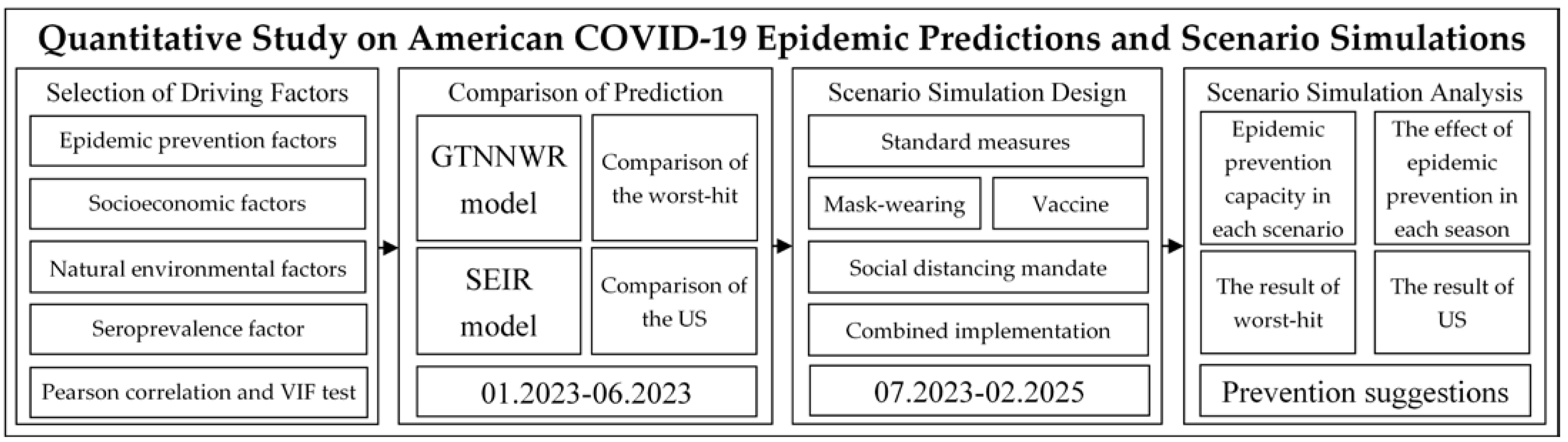
2.3.3. Research Framework

This study included the following four aspects, as shown in Figure 2:
(1)
Selection of Driving Factors: After reviewing the relevant literature, this study selected four categories of driving factors as independent variables. Through Pearson correlation testing and multicollinearity testing, variables suitable for subsequent experiments were chosen.
(2)
Comparison of Prediction: This study designed comparative experiments with the commonly used SEIR model in COVID-19 prediction. It calculated the prediction accuracy of the GTNNWR model and the SEIR model relative to the actual values from January 2023 to June 2023. Comparative analyses were conducted for the 12 states heavily affected by the pandemic and the continental United States.
(3)
Scenario Simulation Design: Based on three health and epidemic prevention factors (mask wearing, vaccination, social distancing mandate), this study designed five scenarios. These scenarios were used as inputs for the GTNNWR model, and the death toll under different scenarios in each state was calculated.
(4)
Scenario Simulation Analysis: This step involved comparing the effectiveness of different scenario prevention measures, comparing the effectiveness of prevention measures in different seasons under the same scenario, and analyzing changes in the number of deaths in worst-hit areas and the continental United States under different scenarios.

3. Results and Discussion

3.1. Data Description and Analysis

Variable selection and data normalization are the keys to the GTNNWR model. This study identified four major driving factors based on the spatiotemporal evolution of deaths in the United States. The key variables were obtained by collinearity test and correlation test, and results are shown in Table 2 and Table 3. All factors are significantly correlated with the dependent variables. Specifically, SDI, SP, Prec, Poverty-p, Elderly-p, Unemp-p, and High-p were positively related to the number of deaths, Masks-p, Vaccinate-p, Temp, WS, m-Income, College-p, Sero-p were negatively related to the number of deaths. Multicollinearity among all factors was tested using VIF values, all VIF values were less than 10, suggesting these 14 factors did not lead to multicollinearity. Therefore, we selected all factors as independent variables in subsequent studies.

3.2. Comparison and Analysis of the Accuracy during the Validation Period

According to the experimental design, SEIR model experiments were conducted in 49 states, and all data from the continental United States were incorporated into the GTNNWR model for experimentation. Through multiple rounds of ten-fold crossover experiments, we selected the experimental results that showed the highest fitting accuracy, the highest generalization accuracy, and the lowest error terms. This study focused on twelve states with the highest number of deaths between the beginning of the epidemic and June 2023, including California, Texas, Florida, New York, Illinois, Pennsylvania, Arizona, Ohio, Georgia, Michigan, New Jersey, and Tennessee. The SEIR and GTNNWR models were used to predict the number of deaths for each month, and the actual data for each state were combined to calculate the relative error. The prediction results of the GTNNWR and SEIR models for the worst-hit states and continental US each month during the validation period are shown in Table 4.
The GTNNWR model outperforms the SEIR model in predicting deaths. Specifically, the average prediction accuracy of the GTNNWR model for the continental United States is 85.7%, while the SEIR model lags behind at 76.9%. In most of the worst-hit states, the GTNNWR model demonstrates higher prediction accuracy than the SEIR model. Additionally, the GTNNWR model exhibits a significant advantage in long-term predictions. In the last month of the validation period, the prediction accuracy of the SEIR model notably declined, primarily falling within the range of 20 to 60%. In contrast, the GTNNWR model maintains a higher prediction accuracy, ranging from 65 to 85%. The GTNNWR model provides a more accurate prediction of future outbreaks, enabling us to implement better control measures in advance and ensure adequate preparation of medical resources.
Figure 3 displays the variation curves of the deaths during the validation period under the GTNNWR and SEIR models. The GTNNWR model exhibits a higher degree of accuracy in capturing the fluctuations, reflecting the ups and downs of the curve more comprehensively. In contrast, the predictions from the SEIR model show a gradual decrease over time, which does not reflect an upward trend. This indicates that the SEIR model did not adequately learn the sudden changes features, resulting in less accurate predictions. The GTNNWR model provides more insightful predictions regarding sudden attacks or mitigation patterns of the epidemic and adds significant reference value, which implies that the GTNNWR model can be a valuable tool for understanding and responding to unexpected changes in the outbreak dynamics, aiding in better preparedness and response strategies.
Other studies indicate that the SEIR model demonstrates high short-term predictive accuracy, reaching 90% within one month, but its accuracy drops to 55% within six months. These conclusions are similar to our study. The speculated reason is that the SEIR model categorizes the population into a few groups, making it challenging to effectively cover all individuals. Additionally, the interactions between different groups are highly complex, making it difficult to solve through the limited partial differential equations in the SEIR model. Furthermore, the preset parameters also change over time, and the model does not promptly update these parameters, resulting in significant errors when using outdated parameters.
The above results indicate that the results obtained from the spatiotemporal weighted neural network method, which incorporates multiple driving factors, demonstrate a qualitative improvement over the traditional infectious disease dynamics model. The SEIR model’s limitation lies in dividing the population into a limited number of categories, which only effectively covers some of the population. The complexity of interactions among different populations makes it challenging to adequately address all aspects with the SEIR model’s small number of partial differential equations. However, the GTNNWR model can extract and account for the intricate non-linear relationships and spatiotemporal heterogeneity between the number of deaths and the driving factors. Utilizing the powerful fitting capacity of deep neural networks, the GTNNWR model delves deep into these complex relationships and spatiotemporal characteristics, uncovering general patterns and rules, leading to a significant improvement in the COVID-19 prediction.

3.3. Prediction and Analysis of COVID-19 during the Predicted Period

Prediction and analysis of the COVID-19 pandemic is the focus of this study. The results show that if more stringent epidemic prevention measures are not taken during the predicted period, 78,000 people may die in the continental United States, including approximately 30,900 in the second half of 2023, approximately 41,000 in 2024, and approximately 6100 from January to February 2025. The distribution of deaths among states in the United States varies significantly. Approximately 46% of the deaths during the predicted period are concentrated in three states, California (19,000 people), Texas (9400 people), and Florida (7900 people), the changes in the worst-hit areas are shown in Figure 4. However, the evolving trend of the epidemic has a positive side. The number of deaths caused by it has gradually decreased year on year, which means that the epidemic is expected to weaken in the next two years while maintaining existing prevention and control measures.
Seasonal factors are still an important objective reason affecting the number of deaths, with winter being the peak period, summer being the trough period, and spring and autumn being in the middle. The average monthly death in the continental United States is 4900 in the winter, only 2800 in the summer, 3800 in the spring, and 4500 in the fall.

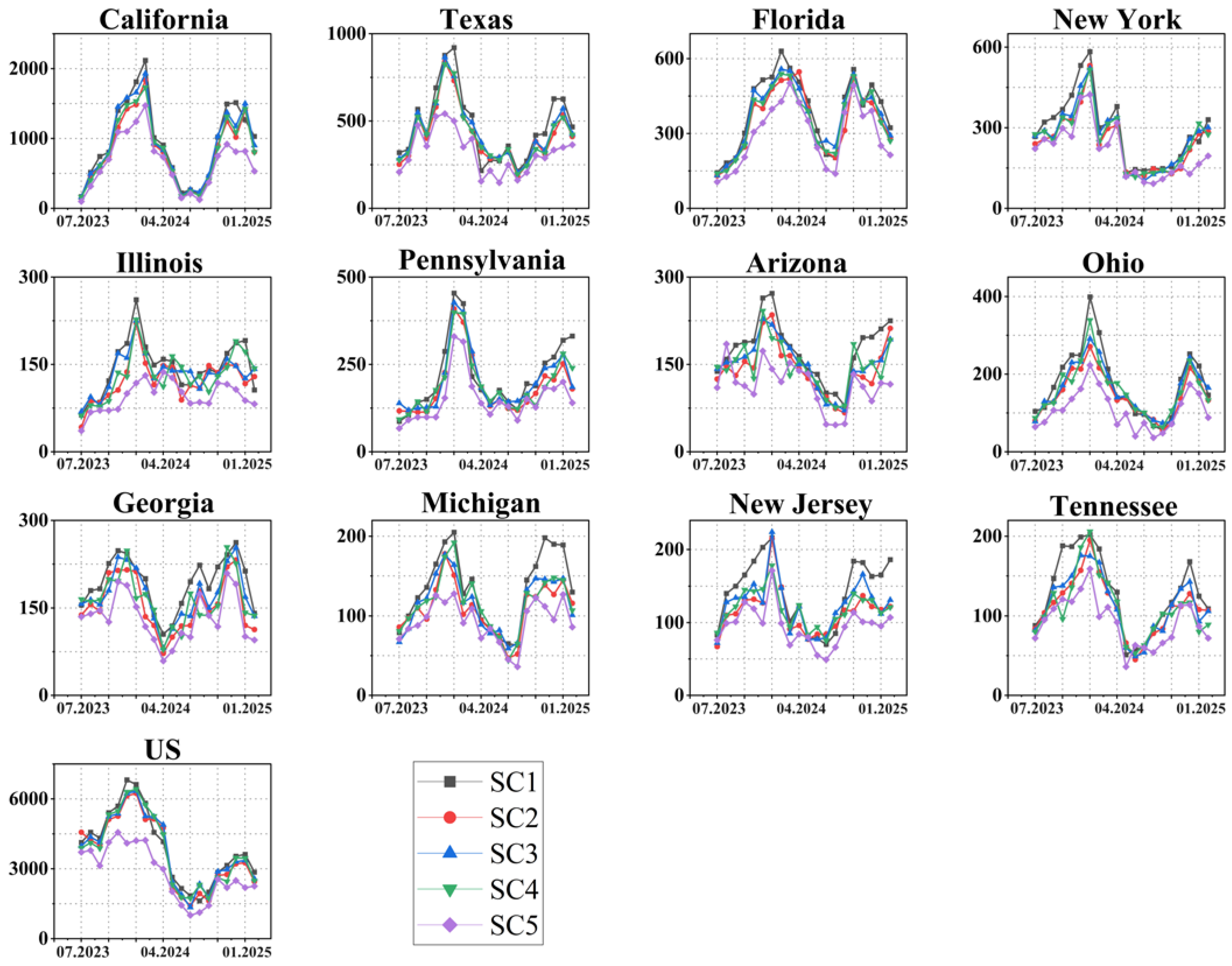
3.4. The COVID-19 Scenario Simulation and Analysis

The purpose of scenario simulation is to measure the impact of different preventive measures and the joint implementation of preventive measures on COVID-19. Figure 5 plots the changing trend of the number of deaths caused by various scenarios during the predicted period. The values of each scenario are ranked as follows:
Scenario 1 represents the most severe situation, resulting in 78,000 deaths.
Scenario 3: The second most severe scenario, with 75,900 deaths.
Scenario 4: The third scenario resulted in 75,200 deaths.
Scenario 2: This scenario leads to 73,800 deaths.
Scenario 5: The least severe scenario, with 56,800 deaths.
The results indicate the effectiveness of different measures in controlling the epidemic: (1) Combined implementation of the three epidemic prevention measures: The best-performing scenario reduced the deaths by approximately 27.2%, which proves 5 to 10 fold more effective than any single stringent measure. (2) The strict implementation of masks: Among the individual health measures, mask wearing showed the most significant effect, reducing the number of deaths by approximately 5.38%. (3) The strict implementation of vaccines: The effect is less pronounced compared to masks, but it still leads to a reduction of approximately 3.59% in the number of deaths. (4) The strict implementation of social distancing mandates: Among the individual health measures, this one has the least impact, reducing the number of deaths by approximately 2.69%. (5) Maintain the current intensity of epidemic prevention: This approach has shown to be the least effective in curbing the number of deaths.
The effectiveness of different policies across states is reflected by the cumulative number of deaths over the predicted period, from July 2023 to mid-February 2025 under Scenario 1, the top five states for deaths were California (19,061), Texas (9405), Florida (7872), New York (5730) and Pennsylvania (4349). Because Scenario 1 is a realistic reflection of a realistic situation and has the greatest relevance, the simulation results for deaths in these states indicate the need to focus on prevention and to devote more healthcare resources. The top five in Scenario 2 were California (16,452), Texas (8334), Florida (7017), New York (4925), and Pennsylvania (3765). The top five in Scenario 3 are California (18,152), Texas (8782), Florida (7439), New York (5238), and Pennsylvania (4038). The top five in Scenario 4 are California (16,798), Texas (8496), Florida (7131), New York (5093), and Pennsylvania (3860). The top five in Scenario 5 were California (13,254), Texas (6403), Florida (5977), New York (4228), and Pennsylvania (3030).
However, in certain months in some states, adopting the strict preventive measures may not guarantee lower deaths than the standard prevention measures, such as in California in January 2025, Florida in August 2024, and March–April 2024 in the continental U.S. Scenario 5, where the strict preventive measures targeting three preventive measures, ensures deaths are lower than that of standard prevention measures. This indicates the “herd immunity” concept often advocated in the United States may not stand up to scrutiny. Without special measures, the deaths in some worst-hit states increase to some extent.
Season not only directly affected the number of deaths, but also affected the number of deaths by affecting the effectiveness of epidemic prevention measures. The mitigation effect of Scenarios 2 to 5 on the epidemic in winter is significantly higher than that in other seasons. Based on Scenario 1, the reduction rate in winter Scenarios 2 to 5 in the continental United States is 9.1%, 8.3%, 5.5% and 45%, 3.8%, 3.2%, 4.6% and 26% in summer, 6.6%, 4.2%, 4.5% and 30% in autumn, 8.1%, 4.7%, 3.0%, 33% in spring. The research found that the combined implementation of measures in mask wearing, vaccination, and social distancing during winter can reduce the deaths by approximately 45%, which is approximately 1.5–3- fold higher than in the other seasons. In future winters, the effect of health and epidemic prevention measures will be more significant. Policy makers should focus on implementing more stringent prevention measures in winter when the epidemic is most severe, and a higher reduction would mean more infections and deaths could be avoided, as well as saving medical funds and resources.
Universal mask usage is a relatively inexpensive and low-impact intervention measure and should be prioritized as a critical option to save lives in the United States. The efficacy of mask wearing has been evident in various widely adopted countries and regions, such as Singapore, the United Kingdom, South Korea, Hong Kong, Japan, and Iceland, where COVID-19 deaths have been significantly reduced or even reduced to zero [5,50,62,66]. However, mask usage has become a contentious issue in the United States. A survey conducted in September 2020 revealed that only 49% of US [67] residents reported consistently wearing masks in public places. In the states with the highest reported usage, such as Virginia, Florida, and California, mask usage was reported at only 60% [68]. According to the results of Scenario 2, by early 2024, masks can significantly suppress the cyclical winter peaks. Achieving and maintaining a 95% mask usage rate in the population may seem challenging, but if this target is reached, there will be significant breakthroughs in preventing and controlling COVID-19. On the other hand, if the existing mask usage rate remains within the range of 30 to 60% for an extended period, any relaxation in government control over outdoor mask wearing would lead to a sharp decline in mask usage that month. Based on this, this study speculates that maintaining a 95% outdoor mask-wearing rate would take a lot of work to sustain.
Currently, the vaccines available on the market for COVID-19 are mainly based on the inactivated SARS-CoV-2 virus, which, when injected into the human immune system, elicits the production of corresponding antibodies, thus achieving immunity. This study validates the effectiveness of vaccination in epidemic prevention and control. However, the debate over vaccines has been long-standing. Since the pandemic outbreak, the SARS-CoV-2 virus has undergone several mutations, including Alpha, Beta, Gamma, Delta, and Omicron variants. The Omicron variant, which emerged at the end of 2021, has a transmission capability 5-fold higher than the Delta variant [69]. Due to these mutations, the existing vaccines have shown reduced protection against infection and death from these new variants [7,70], leading to cases of reinfection among vaccinated individuals and recovered COVID-19 patients [7,71], particularly in the context of the Delta and Omicron variants [9]. High vaccination rates in countries like Israel and the UK have seen a significant resurgence of COVID-19 cases [9]. Some studies have also indicated the immunity conferred by vaccines against the Delta variant decreases after receiving the second dose [71]. These findings suggest that the current vaccine administration might not generate sufficient and adequate antibodies to entirely prevent virus infection. To tackle these challenges, many countries are now adopting vaccine booster shots [9], which involve using additional doses of the vaccine to raise the levels of antibodies in the immune system, thus countering the impact of rapidly mutating strains. In this study, the term “vaccine complete vaccination rate” includes administering vaccine booster shots, aiming to investigate whether it has an immunological effect on rapidly mutating strains. The results of Scenario 4 indicated that accelerating vaccine administration is having a significant impact on epidemic prevention and reduces deaths, even in the presence of virus mutations. Booster shots are also considered a cost-saving strategy in the US [72], with the cost–benefit ratio being 1.95. For every USD 1 invested in booster shots, USD 2 will be saved in future treatment costs (hospitalization expenses due to COVID-19 infection). In conclusion, vaccination not only significantly impacts epidemic prevention but also offers cost advantages and enjoys relatively high public acceptance. Therefore, it is worth promoting vigorously.
Maintaining social distancing is a crucial preventive measure in public health, primarily aimed at warning individuals to stay away from large gatherings and reducing close contact during indoor and outdoor interactions. By doing so, it helps to minimize the spread of the pandemic. In the context of COVID-19 prevention and control, maintaining social distancing has played a significant role and has been widely adopted worldwide as a primary measure for COVID-19 prevention. Some researchers refer to this measure as “flattening the curve” [73], implying that by adhering to social distancing guidelines, the exponential increase in infection and death rates can be slowed down or even reversed. Scenario 3 explicitly explores the hypothesis of maintaining social distancing, and under the assumption that COVID-19 will gradually subside over the next year and a half, it further reduces the deaths. This validates the belief that maintaining social distancing can alleviate the impact of the pandemic. However, it is worth noting that the effectiveness of Scenario 3 is not as significant as Scenario 2 and Scenario 4 in the overall context of the United States and most COVID-19 hotspots within the country. Additionally, in some states and during specific months, the predicted deaths under Scenario 3 are higher than in Scenario 1. This suggests that solely relying on maintaining social distancing without implementing other preventive measures or continuing their growth could lead to adverse consequences in certain states. In conclusion, maintaining social distancing has played a vital role in mitigating the COVID-19 pandemic and has been recognized as a primary measure for prevention and control worldwide. However, it is essential to understand that in some situations, especially when used in isolation, its effectiveness may not be as substantial as when combined with other preventive measures. Therefore, a comprehensive and integrated approach to pandemic prevention is necessary to achieve the most effective results.

4. Conclusions

This study focuses on the prediction and scenario simulation of the deaths caused by the COVID-19 epidemic by taking the time and space information into account and combining it with a variety of driving factors, discusses the changes in the number of deaths under different prevention and control measures and their combined implementation, improve the prediction accuracy and find suitable strategies for the prevention and control of the epidemic. The research results reveal a 9% improvement in prediction accuracy using the GTNNWR model compared to the SEIR model. It indicated the effectiveness of measures such as mask-wearing, vaccination, and maintaining social distance, with reductions in deaths of 5.38%, 3.59%, 2.69%, and 27.2%, respectively. The combined implementation of preventive measures not only reduces deaths by more than 20% but also ensures that the number of deaths does not exceed those standard preventive measures in any month and state. During winter, the impact of four preventive scenarios is more significant, leading to larger reductions in deaths (9.1%, 8.3%, 5.5%, and 45%) compared to other seasons.
The deficiencies and prospects of this study are mainly in the large time scale leads to loopholes, we used month as the minimum unit in this study. However, if the epidemic suddenly broke out within one month, this study could not catch it in time, which would have a serious loophole and an adverse impact on the prevention and control of the epidemic. Subsequent studies can fill in the daily driving factors through interpolation and match the independent variables with the dependent variables, to construct a prediction model of the COVID-19 epidemic daily.

Author Contributions

Jingtao Sun was involved in the design of this study, and interpretation of data, drafted the major revisions, performed the experiments, and completed the overall writing; Jin Qi conceived part of the experiments and polished the writing; Zhen Yan drafted part of the manuscript and polished the writing; Yadong Li conceived part of the experiments and improved the manuscript; Jie Liang was involved in the revision of the manuscript; Sensen Wu contributed to the study design and algorithm improvement; All authors have read and agreed to the published version of the manuscript.

Funding

This work was supported by the National Key Research and Development Program of China (grant 2021YFB3900900), funded by the Ministry of Science and Technology of the People’s Republic of China, the grantee is Sensen Wu; the National Natural Science Foundation of China (Grant No. 72073118), funded by National Natural Science Foundation of China, the grantee is Zhen Yan; the Key Research Projects of Humanities and Social Sciences under the 14th Five-Year Plan of the Ministry of Education (22JJD790079), funded by National Natural Science Foundation of China, the grantee is Zhen Yan; the Provincial Key R&D Program of Zhejiang (grant 2021C01031), funded by Department of Science and Technology of Zhejiang Province, the grantee is Sensen Wu; the Deep-time Digital Earth (DDE) Big Science Program, funded by China Geological Survey (CGS), British Geological Survey (BGS), Russian Geological Research Institute (VSEGEI), International Commission on Stratigraphy (ICS), Commission on the Management & Application of Geoscience Information (CGI), American Association of Petroleum Geologists (AAPG), International Association of Mathematical Geosciences (IAMG), International Association on the Genesis of Ore Deposits (IAGOD), Commission of Geological Map of the World (CGMW), International Association of Geomorphologists (IAG), International Palaeontological Association (IPA), and International Association of Sedimentologists (IAS), the grantee is Jin Qi.

Data Availability Statement

The data presented in this study are available on request from the corresponding author. The data are not publicly available due to restrictions imposed by the privacy approval and informed consent agreements with study participants.

Acknowledgments

The authors would like to thank the support from our university and laboratory and thank all anonymous reviewers for their constructive comments that improved this paper.

Conflicts of Interest

The authors declare no conflict of interest.

Correction Statement

This article has been republished with a minor correction to the Data Availability Statement. This change does not affect the scientific content of the article.

References

  1. Modeling COVID-19 scenarios for the United States. Nat. Med. 2021, 27, 94–105. [CrossRef]
  2. Ciotti, M.; Angeletti, S.; Minieri, M.; Giovannetti, M.; Benvenuto, D.; Pascarella, S.; Sagnelli, C.; Bianchi, M.; Bernardini, S.; Ciccozzi, M. COVID-19 outbreak: An overview. Chemotherapy 2020, 64, 215–223. [Google Scholar] [CrossRef] [PubMed]
  3. Ciotti, M.; Ciccozzi, M.; Terrinoni, A.; Jiang, W.-C.; Wang, C.-B.; Bernardini, S. The COVID-19 pandemic. Crit. Rev. Clin. Lab. Sci. 2020, 57, 365–388. [Google Scholar] [CrossRef]
  4. Coronavirus Disease 2019 (COVID-19). p. CDC Provides Credible COVID-19 Health Information to the U.S. Available online: https://www.cdc.gov/coronavirus/2019-ncov/index.html (accessed on 9 January 2024).
  5. Betsch, C.; Korn, L.; Sprengholz, P.; Felgendreff, L.; Eitze, S.; Schmid, P.; Böhm, R. Social and behavioral consequences of mask policies during the COVID-19 pandemic. Proc. Natl. Acad. Sci. USA 2020, 117, 21851–21853. [Google Scholar] [CrossRef]
  6. Chu, D.K.; Akl, E.A.; Duda, S.; Solo, K.; Yaacoub, S.; Schünemann, H.J. Physical distancing, face masks, and eye protection to prevent person-to-person transmission of SARS-CoV-2 and COVID-19: A systematic review and meta-analysis. Lancet 2020, 395, 1973–1987. [Google Scholar] [CrossRef] [PubMed]
  7. Cohn, B.A.; Cirillo, P.M.; Murphy, C.C.; Krigbaum, N.Y.; Wallace, A.W. SARS-CoV-2 vaccine protection and deaths among US veterans during 2021. Science 2022, 375, 331–336. [Google Scholar] [CrossRef] [PubMed]
  8. Folegatti, P.M.; Ewer, K.J.; Aley, P.K.; Angus, B.; Becker, S.; Belij-Rammerstorfer, S.; Bellamy, D.; Bibi, S.; Bittaye, M.; Clutterbuck, E.A.; et al. Safety and immunogenicity of the ChAdOx1 nCoV-19 vaccine against SARS-CoV-2: A preliminary report of a phase 1/2, single-blind, randomised controlled trial. Lancet 2020, 396, 467–478. [Google Scholar] [CrossRef]
  9. Barda, N.; Dagan, N.; Cohen, C.; A Hernán, M.; Lipsitch, M.; Kohane, I.S.; Reis, B.Y.; Balicer, R.D. Effectiveness of a third dose of the BNT162b2 mRNA COVID-19 vaccine for preventing severe outcomes in Israel: An observational study. Lancet 2021, 398, 2093–2100. [Google Scholar] [CrossRef]
  10. Mccafferty, S.; Ashley, S. Covid-19 Social Distancing Interventions by Statutory Mandate and Their Observational Correlation to Mortality in the United States and Europe. Pragmat. Obs. Res. 2021, 12, 15–24. [Google Scholar] [CrossRef]
  11. Ganesapillai, M.; Mondal, B.; Sarkar, I.; Sinha, A.; Ray, S.S.; Kwon, Y.-N.; Nakamura, K.; Govardhan, K. The face behind the Covid-19 mask-A comprehensive review. Environ. Technol. Innov. 2022, 28, 102837. [Google Scholar] [CrossRef]
  12. Notarte, K.I.; Catahay, J.A.; Velasco, J.V.; Pastrana, A.; Ver, A.T.; Pangilinan, F.C.; Peligro, P.J.; Casimiro, M.; Guerrero, J.J.; Gellaco, M.M.L.; et al. Impact of COVID-19 vaccination on the risk of developing long-COVID and on existing long-COVID symptoms: A systematic review. EClinicalMedicine 2022, 53, 101624. [Google Scholar] [CrossRef] [PubMed]
  13. Saha, S.; Samanta, G.; Nieto, J.J. Impact of optimal vaccination and social distancing on COVID-19 pandemic. Math. Comput. Simul. 2022, 200, 285–314. [Google Scholar] [CrossRef] [PubMed]
  14. Feyisa, H.L. The World Economy at COVID-19 quarantine: Contemporary review. Int. J. Econ. Financ. Manag. Sci. 2020, 8, 63–74. [Google Scholar]
  15. Chakraborty, I.; Maity, P. COVID-19 outbreak: Migration, effects on society, global environment and prevention. Sci. Total Environ. 2020, 728, 138882. [Google Scholar] [CrossRef] [PubMed]
  16. Yao, H.; Chen, J.H.; Xu, Y.F. Patients with mental health disorders in the COVID-19 epidemic. Lancet Psychiatry 2020, 7, e21. [Google Scholar] [CrossRef]
  17. Flores, A.; Cole, J.C.; Dickert, S.; Eom, K.; Jiga-Boy, G.M.; Kogut, T.; Loria, R.; Mayorga, M.; Pedersen, E.J.; Pereira, B.; et al. Politicians polarize and experts depolarize public support for COVID-19 management policies across countries. Proc. Natl. Acad. Sci. USA 2022, 119, e2117543119. [Google Scholar] [CrossRef] [PubMed]
  18. Gallo, M.B.; Aghagoli, G.; Lavine, K.; Yang, L.; Siff, E.J.; Chiang, S.S.; Salazar-Mather, T.P.; Dumenco, L.; Savaria, M.C.; Aung, S.N.; et al. Predictors of COVID-19 severity: A literature review. Rev. Med. Virol. 2021, 31, 1–10. [Google Scholar] [CrossRef]
  19. Rahman, M.; Paul, K.C.; Hossain, A.; Ali, G.G.M.N.; Rahman, S.; Thill, J.-C. Machine Learning on the COVID-19 Pandemic, Human Mobility and Air Quality: A Review. IEEE Access 2021, 9, 72420–72450. [Google Scholar] [CrossRef]
  20. Wynants, L.; Van Calster, B.; Collins, G.S.; Riley, R.D.; Heinze, G.; Schuit, E.; Bonten, M.M.J.; Dahly, D.L.; Damen, J.A.; Debray, T.P.A.; et al. Prediction models for diagnosis and prognosis of covid-19: Systematic review and critical appraisal. BMJ 2020, 369, m1328. [Google Scholar] [CrossRef]
  21. Swapnarekha, H.; Behera, H.S.; Nayak, J.; Naik, B. Role of intelligent computing in COVID-19 prognosis: A state-of-the-art review. Chaos Solitons Fractals 2020, 138, 109947. [Google Scholar] [CrossRef]
  22. Xiang, Y.; Jia, Y.; Chen, L.; Guo, L.; Shu, B.; Long, E. COVID-19 epidemic prediction and the impact of public health interventions: A review of COVID-19 epidemic models. Infect. Dis. Model. 2021, 6, 324–342. [Google Scholar] [CrossRef] [PubMed]
  23. Xi, J.; Liu, X.; Wang, J.; Yao, L.; Zhou, C. A Systematic Review of COVID-19 Geographical Research: Machine Learning and Bibliometric Approach. Ann. Am. Assoc. Geogr. 2023, 113, 581–598. [Google Scholar] [CrossRef]
  24. Isazade, V.; Qasimi, A.B.; Dong, P.; Kaplan, G.; Isazade, E. Integration of Moran’s I, geographically weighted regression (GWR), and ordinary least square (OLS) models in spatiotemporal modeling of COVID-19 outbreak in Qom and Mazandaran provinces, Iran. Model. Earth Syst. Environ. 2023, 9, 3923–3937. [Google Scholar] [CrossRef] [PubMed]
  25. Ardiyanto, R.; Indra, T.L.; Manesa, M.D.M. Geospatial approach to accessibility of referral hospitals using geometric network analysts and spatial distribution models of Covid-19 spread cases based on GIS in Bekasi City, West Java. Indones. J. Geogr. 2022, 54, 173–184. [Google Scholar] [CrossRef]
  26. Rasul, A.; Balzter, H. The Role of Climate in the Spread of COVID-19 in Different Latitudes across the World. COVID 2022, 2, 1183–1192. [Google Scholar] [CrossRef]
  27. Qiao, M.; Huang, B. Studying the spatiotemporal impacts of socio-demographic and mobility-related factors to predict the spread of COVID-19. Cities 2023, 138, 104360. [Google Scholar] [CrossRef] [PubMed]
  28. Qiao, M.; Huang, B. COVID-19 spread prediction using socio-demographic and mobility-related data. Cities 2023, 138, 104360. [Google Scholar] [CrossRef] [PubMed]
  29. Sifriyani, S.; Rasjid, M.; Rosadi, D.; Anwar, S.; Wahyuni, R.D.; Jalaluddin, S. Spatial-temporal epidemiology of COVID-19 Using a geographically and temporally weighted regression model. Symmetry 2022, 14, 742. [Google Scholar] [CrossRef]
  30. Manyangadze, T.; Chimbari, M.J.; Gebreslasie, M.; Mukaratirwa, S. Risk factors and micro-geographical heterogeneity of Schistosoma haematobium in Ndumo area, uMkhanyakude district, KwaZulu-Natal, South Africa. Acta Trop. 2016, 159, 176–184. [Google Scholar] [CrossRef]
  31. Mohammadinia, A.; Saeidian, B.; Pradhan, B.; Ghaemi, Z. Prediction mapping of human leptospirosis using ANN, GWR, SVM and GLM approaches. BMC Infect. Dis. 2019, 19, 971. [Google Scholar] [CrossRef]
  32. Halim, S.; Octavia, T.; Handojo, A. Dengue fever outbreak prediction in Surabaya using a geographically weighted regression. In Proceedings of the 2019 4th Technology Innovation Management and Engineering Science International Conference (TIMES-iCON), Bangkok, Thailand, 11–13 December 2019. [Google Scholar]
  33. Ahangarcani, M.; Farnaghi, M.; Shirzadi, M.R. Predictive Map of Spatio-Temporal Distribution of Leptospirosis Using Geographical Weighted Regression and Multilayer Perceptron Neural Network Methods. J. Geomat. Sci. Technol. 2016, 6, 79–98. [Google Scholar]
  34. Sollers, K.; Liu, X.; Martínez-López, B. An implementation of Geographical and Temporal Weighted Regression in modeling occurrences of Porcine Reproductive and Respiratory Syndrome in the US swine industry. Front. Vet. Sci. 2019. [Google Scholar] [CrossRef]
  35. Kolesnikov, A.A.; Kikin, P.M.; Portnov, A.M. Diseases spread prediction in tropical areas by machine learning methods ensembling and spatial analysis techniques. Int. Arch. Photogramm. Remote Sens. Spat. Inf. Sci. 2019, 42, 221–226. [Google Scholar] [CrossRef]
  36. Du, Z.; Wang, Z.; Wu, S.; Zhang, F.; Liu, R. Geographically neural network weighted regression for the accurate estimation of spatial non-stationarity. Int. J. Geogr. Inf. Sci. 2020, 34, 1353–1377. [Google Scholar] [CrossRef]
  37. Miao, L.; Tang, S.; Li, X.; Yu, D.; Deng, Y.; Hang, T.; Yang, H.; Liang, Y.; Kwan, M.-P.; Huang, L. Estimating the CO2 emissions of Chinese cities from 2011 to 2020 based on SPNN-GNNWR. Environ. Res. 2023, 218, 115060. [Google Scholar] [CrossRef] [PubMed]
  38. Liang, M.; Zhang, L.; Wu, S.; Zhu, Y.; Dai, Z.; Wang, Y.; Qi, J.; Chen, Y.; Du, Z. A High-Resolution Land Surface Temperature Downscaling Method Based on Geographically Weighted Neural Network Regression. Remote Sens. 2023, 15, 1740. [Google Scholar] [CrossRef]
  39. Qi, J.; Du, Z.; Wu, S.; Chen, Y.; Wang, Y. A spatiotemporally weighted intelligent method for exploring fine-scale distributions of surface dissolved silicate in coastal seas. Sci. Total Environ. 2023, 886, 163981. [Google Scholar] [CrossRef]
  40. Liu, C.; Wu, S.; Dai, Z.; Wang, Y.; Du, Z.; Liu, X.; Qiu, C. High-Resolution Daily Spatiotemporal Distribution and Evaluation of Ground-Level Nitrogen Dioxide Concentration in the Beijing-Tianjin-Hebei Region Based on TROPOMI Data. Remote Sens. 2023, 15, 3878. [Google Scholar] [CrossRef]
  41. Fanelli, D.; Piazza, F. Analysis and forecast of COVID-19 spreading in China, Italy and France. Chaos Solitons Fractals 2020, 134, 109761. [Google Scholar] [CrossRef]
  42. Hou, X.; Gao, S.; Li, Q.; Kang, Y.; Chen, N.; Chen, K.; Rao, J.; Ellenberg, J.S.; Patz, J.A. Intracounty modeling of COVID-19 infection with human mobility: Assessing spatial heterogeneity with business traffic, age, and race. Proc. Natl. Acad. Sci. USA 2021, 118, e2020524118. [Google Scholar] [CrossRef]
  43. Tang, B.; Bragazzi, N.L.; Li, Q.; Tang, S.; Xiao, Y.; Wu, J. An updated estimation of the risk of transmission of the novel coronavirus (2019-nCov). Infect. Dis. Model. 2020, 5, 248–255. [Google Scholar] [CrossRef] [PubMed]
  44. Zhao, S.; Lin, Q.; Ran, J.; Musa, S.S.; Yang, G.; Wang, W.; Lou, Y.; Gao, D.; Yang, L.; He, D.; et al. Preliminary estimation of the basic reproduction number of novel coronavirus (2019-nCoV) in China, from 2019 to 2020: A data-driven analysis in the early phase of the outbreak. Int. J. Infect. Dis. 2020, 92, 214–217. [Google Scholar] [CrossRef]
  45. Choi, S.; Ki, M. Estimating the reproductive number and the outbreak size of COVID-19 in Korea. Epidemiol. Health 2020, 42, e2020011. [Google Scholar] [CrossRef]
  46. Chimmula, V.; Zhang, L. Time series forecasting of COVID-19 transmission in Canada using LSTM networks. Chaos Solitons Fractals 2020, 135, 109864. [Google Scholar] [CrossRef] [PubMed]
  47. Soures, N.; Chambers, D.; Carmichael, Z.; Daram, A.; Shah, D.P.; Clark, K.; Potter, L.; Kudithipudi, D. SIRNet: Understanding social distancing measures with hybrid neural network model for COVID-19 infectious spread. arXiv 2020, arXiv:2004.10376. [Google Scholar]
  48. Wang, D.; Wang, D.; Zuo, F.; Gao, J.; He, Y.; Bian, Z.; Bernardes, S.D.; Na, C.; Wang, J.; Petinos, J.; et al. Agent-based simulation model and deep learning techniques to evaluate and predict transportation trends around COVID-19. arXiv 2020, arXiv:2010.09648. [Google Scholar]
  49. Kai, D.; Kai, D.; Goldstein, G.-P.; Morgunov, A.; Nangalia, V.; Rotkirch, A. Universal masking is urgent in the COVID-19 pandemic: SEIR and agent based models, empirical validation, policy recommendations. arXiv 2020, arXiv:2004.13553. [Google Scholar]
  50. Panovska-Griffiths, J.; Kerr, C.C.; Waites, W.; Stuart, R.M.; Mistry, D.; Foster, D.; Klein, D.J.; Viner, R.M.; Bonell, C. Modelling the potential impact of mask use in schools and society on COVID-19 control in the UK. Sci. Rep. 2021, 11, 8747. [Google Scholar] [CrossRef]
  51. Vinceti, M.; Filippini, T.; Rothman, K.J.; Ferrari, F.; Goffi, A.; Maffeis, G.; Orsini, N. Lockdown timing and efficacy in controlling COVID-19 using mobile phone tracking. EClinicalMedicine 2020, 25, 100457. [Google Scholar] [CrossRef]
  52. Spada, A.; Tucci, F.A.; Ummarino, A.; Ciavarella, P.P.; Calà, N.; Troiano, V.; Caputo, M.; Ianzano, R.; Corbo, S.; de Biase, M.; et al. Structural equation modeling to shed light on the controversial role of climate on the spread of SARS-CoV-2. Sci. Rep. 2021, 11, 8358. [Google Scholar] [CrossRef]
  53. Dutta, B.K.; King, W.R. A competitive scenario modeling system. Manag. Sci. 1980, 26, 261–273. [Google Scholar] [CrossRef]
  54. Lemaitre, J.C.; Grantz, K.H.; Kaminsky, J.; Meredith, H.R.; Truelove, S.A.; Lauer, S.A.; Keegan, L.T.; Shah, S.; Wills, J.; Kaminsky, K.; et al. A scenario modeling pipeline for COVID-19 emergency planning. Sci. Rep. 2021, 11, 7534. [Google Scholar] [CrossRef] [PubMed]
  55. Patel, M.D.; Rosenstrom, E.; Ivy, J.S.; Mayorga, M.E.; Keskinocak, P.; Boyce, R.M.; Lich, K.H.; Smith, R.L., 3rd; Johnson, K.T.; Delamater, P.L.; et al. Association of simulated COVID-19 vaccination and nonpharmaceutical interventions with infections, hospitalizations, and mortality. JAMA Netw. Open 2021, 4, e2110782. [Google Scholar] [CrossRef]
  56. Francesco, P.; Lorenzo, Z.; Maurizio, P.; Alessandro, R. Modelling and predicting the effect of social distancing and travel restrictions on COVID-19 spreading. J. R. Soc. Interface 2021, 18, 20200875. [Google Scholar]
  57. Zhang, Y.; Yu, X.; Sun, H.; Tick, G.R.; Wei, W.; Jin, B. COVID-19 infection and recovery in various countries: Modeling the dynamics and evaluating the non-pharmaceutical mitigation scenarios. arXiv 2020, arXiv:2003.13901. [Google Scholar]
  58. Leung, N.H.L.; Chu, D.K.W.; Shiu, E.Y.C.; Chan, K.-H.; McDevitt, J.J.; Hau, B.J.P.; Yen, H.-L.; Li, Y.; Ip, D.K.M.; Peiris, J.S.M.; et al. Respiratory virus shedding in exhaled breath and efficacy of face masks. Nat. Med. 2020, 26, 676–680. [Google Scholar] [CrossRef]
  59. Wake, A.D. The Willingness to Receive COVID-19 Vaccine and Its Associated Factors: “Vaccination Refusal Could Prolong the War of This Pandemic”—A Systematic Review. Risk Manag. Healthc. Policy 2021, 14, 2609–2623. [Google Scholar] [CrossRef]
  60. Wheeler, D.; Tiefelsdorf, M.; Fischer, M.M. Multicollinearity and correlation among local regression coefficients in geographically weighted regression. J. Geogr. Syst. 2005, 7, 161–187. [Google Scholar] [CrossRef]
  61. Wu, S.; Wang, Z.; Du, Z.; Huang, B.; Zhang, F.; Liu, R. Geographically and temporally neural network weighted regression for modeling spatiotemporal non-stationary relationships. Int. J. Geogr. Inf. Sci. 2021, 35, 582–608. [Google Scholar] [CrossRef]
  62. Tirupathi, R.; Bharathidasan, K.; Palabindala, V.; Salim, S.A.; Al-Tawfiq, J.A. Comprehensive review of mask utility and challenges during the COVID-19 pandemic. Infez. Med. 2020, 28 (Suppl. S1), 57–63. [Google Scholar]
  63. Fotheringham, A.S.; Brunsdon, C.; Charlton, M. Geographically Weighted Regression: The Analysis of Spatially Varying Relationships; John Wiley & Sons: Chichester, UK, 2003. [Google Scholar]
  64. Brunsdon, C.; Fotheringham, S.; Charlton, M. Geographically weighted regression. J. R. Stat. Soc. Ser. D Stat. 1998, 47, 431–443. [Google Scholar] [CrossRef]
  65. Brunsdon, C.; Fotheringham, A.S.; Charlton, M.E. Geographically weighted regression: A method for exploring spatial nonstationarity. Geogr. Anal. 1996, 28, 281–298. [Google Scholar] [CrossRef]
  66. Ngonghala, C.N.; Knitter, J.R.; Marinacci, L.; Bonds, M.H.; Gumel, A.B. Assessing the impact of widespread respirator use in curtailing COVID-19 transmission in the USA. R. Soc. Open Sci. 2021, 8, 210699. [Google Scholar] [CrossRef] [PubMed]
  67. Arellano-Cotrina, J.J.; Marengo-Coronel, N.; Atoche-Socola, K.J.; Peña-Soto, C.; Arriola-Guillén, L.E. Effectiveness and Recommendations for the Use of Dental Masks in the Prevention of COVID-19: A Literature Review. Disaster Med. Public Health Prep. 2021, 15, e43–e48. [Google Scholar] [CrossRef] [PubMed]
  68. IHME|COVID-19 Projections. p. Explore Forecasts of COVID-19 Cases, Deaths, and Hospital Resource Use. Available online: https://covid19.healthdata.org/united-states-of-america?view=mask-use&tab=trend (accessed on 9 January 2024).
  69. Fan, Y.; Li, X.; Zhang, L.; Wan, S.; Zhang, L.; Zhou, F. SARS-CoV-2 Omicron variant: Recent progress and future perspectives. Signal Transduct. Target. Ther. 2022, 7, 141. [Google Scholar] [CrossRef] [PubMed]
  70. Bergwerk, M.; Gonen, T.; Lustig, Y.; Amit, S.; Lipsitch, M.; Cohen, C.; Mandelboim, M.; Levin, E.G.; Rubin, C.; Indenbaum, V.; et al. Covid-19 Breakthrough Infections in Vaccinated Health Care Workers. N. Engl. J. Med. 2021, 385, 1474–1484. [Google Scholar] [CrossRef]
  71. Goldberg, Y.; Mandel, M.; Bar-On, Y.M.; Bodenheimer, O.; Freedman, L.; Haas, E.J.; Milo, R.; Alroy-Preis, S.; Ash, N.; Huppert, A. Waning Immunity after the BNT162b2 Vaccine in Israel. N. Engl. J. Med. 2021, 385, e85. [Google Scholar] [CrossRef]
  72. Li, R.; Liu, H.; Fairley, C.K.; Zou, Z.; Xie, L.; Li, X.; Shen, M.; Li, Y.; Zhang, L. Cost-effectiveness analysis of BNT162b2 COVID-19 booster vaccination in the United States. Int. J. Infect. Dis. 2022, 119, 87–94. [Google Scholar] [CrossRef]
  73. Chi, Y.; Wang, Q.; Chen, G.; Zheng, S. The Long-Term Presence of SARS-CoV-2 on Cold-Chain Food Packaging Surfaces Indicates a New COVID-19 Winter Outbreak: A Mini Review. Front. Public Health 2021, 9, 650493. [Google Scholar] [CrossRef]
Figure 1. The implementation procedure of scenario simulation.
Ijgi 13 00031 g001
Figure 2. The research flowchart.
Ijgi 13 00031 g002
Figure 3. The predicted and actual values of deaths from two models in the worst-hit states and continental United States (the horizontal axis is the month, from January 2023; the vertical axis is the number of deaths).
Ijgi 13 00031 g003
Figure 4. Changes in the number of deaths in the worst-hit states and continental United States during the prediction period (the horizontal axis is the month, from July 2023; the vertical axis is the number of deaths).
Ijgi 13 00031 g004
Figure 5. Scenario simulation of the deaths in the worst-hit states and continental United States during the perdition period (the horizontal axis is the month; the vertical axis is the number of deaths).
Ijgi 13 00031 g005
Table 1. The variables and their descriptions in research.
VariablesRepresentations of VariablesUnitsAbbreviations
Dependent
variable
Number of deaths--
Epidemic prevention
factors
The outdoor mask usage rate%Masks-p
Social distancing index-SDI
Total vaccination coverage rate%Vaccinate-p
Natural environmental
factors
Temperature°CTemp
Wind speedm/sWS
Surface pressure%SP
PrecipitationmillimeterPrec
The poverty rate%Poverty-p
The proportion of elderly population%Elder-p
The unemployment rate%Unemp-p
Socioeconomic factorsThe median household incomedollarm-Income
The percentage of population with a college degree%College-p
The percentage of population that did not complete high school%High-p
SeroprevalenceThe percentage of population that had been infected by COVID-19%Sero-p
Table 2. Pearson correlation coefficient between each factor and the deaths of COVID-19.
IndependentMasks-pSDIVaccinate-pTempWSSPPrecPoverty-pElder-pUnemp-pm-IncomeCollege-pHigh-pSero-p
Dependent
04.2020–06.2023−0.268 **0.316 **−0.378 **−0.209 **−0.264 *0.242 **0.201 **0.313 **0.358 *0.326 **−0.247 **−0.177 **0.254 **−0.439 **
** Stands for significance at the 1% level. * Stands for significance at the 5% level.
Table 3. The VIF value of multicollinearity testing of potential risks.
IndependentMasks-pSDIVaccinate-pTempWSSPPrecPoverty-pElder-pUnemp-pm-IncomeCollege-pHigh-pSero-p
Dependent
04.2020–06.20238.6544.2236.3219.3366.2355.6812.3982.3148.2275.3122.6938.3611.6845.255
Table 4. The predictive accuracy of the two models during the validation period for COVID-19 worst-hit states and the continental United States.
ModelsMonthsCATXFLNYILPAAZOHGAMINJTNUS
01.202392.1%95.8%91.1%95.1%90.7%91.1%88.6%87.6%86.8%87.7%87.4%86.6%91.0%
02.202385.6%84.6%82.8%81.8%76.6%83.9%92.2%75.7%81.0%75.0%89.5%81.2%91.5%
GTNNWR03.202381.9%82.0%87.1%76.0%89.5%76.0%84.7%81.1%78.4%79.1%89.6%85.3%87.2%
04.202372.7%78.8%83.5%81.0%78.2%86.5%83.9%74.4%69.0%83.3%79.8%75.6%87.4%
05.202359.6%69.5%83.2%72.9%69.6%80.0%77.3%81.5%77.9%72.3%75.7%72.2%74.7%
06.202368.6%73.8%74.4%79.0%79.2%78.4%84.8%67.7%66.7%68.7%80.0%77.6%82.6%
01.202380.30%83.80%63.00%74.30%78.20%88.40%79.70%78.30%72.90%76.60%82.40%78.10%75.80%
02.202332.10%62.70%62.70%71.20%49.20%58.10%79.10%40.10%59.30%49.30%82.90%76.00%76.10%
SEIR03.202347.90%65.10%81.30%75.40%71.90%62.80%77.10%75.00%44.20%53.70%71.00%74.50%80.60%
04.202352.10%52.00%68.70%64.10%56.90%79.60%76.60%60.40%31.00%72.40%37.10%71.20%83.00%
05.202326.50%58.70%59.60%53.50%41.30%65.90%52.10%33.80%32.60%50.70%44.30%56.70%67.70%
06.202331.00%59.80%53.40%63.00%58.50%41.20%62.10%58.30%23.50%50.60%20.00%65.50%78.70%
Disclaimer/Publisher’s Note: The statements, opinions and data contained in all publications are solely those of the individual author(s) and contributor(s) and not of MDPI and/or the editor(s). MDPI and/or the editor(s) disclaim responsibility for any injury to people or property resulting from any ideas, methods, instructions or products referred to in the content.

