

Analysis of the Spatiotemporal Urban Expansion of the Rome Coastline through GEE and RF Algorithm, Using Landsat Imagery
 ,
,  ,
,  ,
, 
 and
and 
Abstract
1. Introduction
2. Materials and Methods
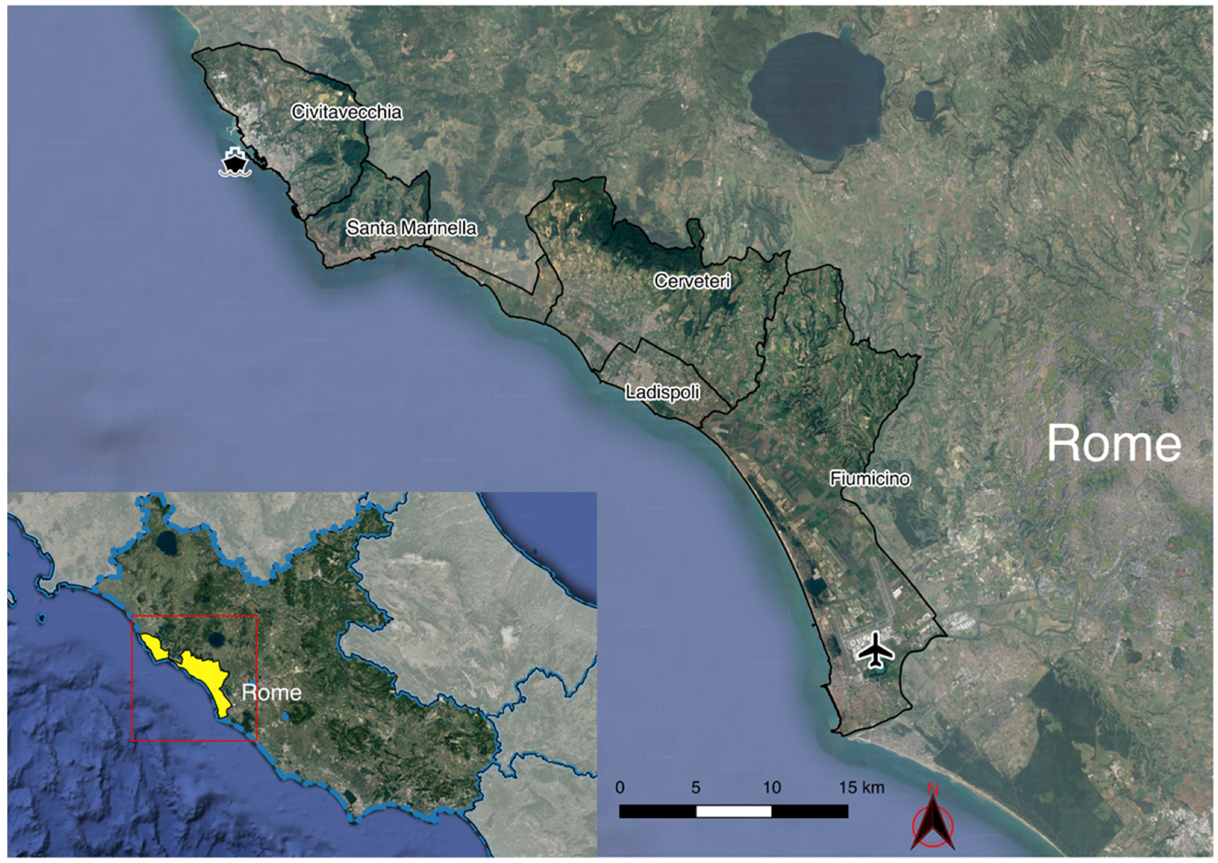
2.1. Study Area
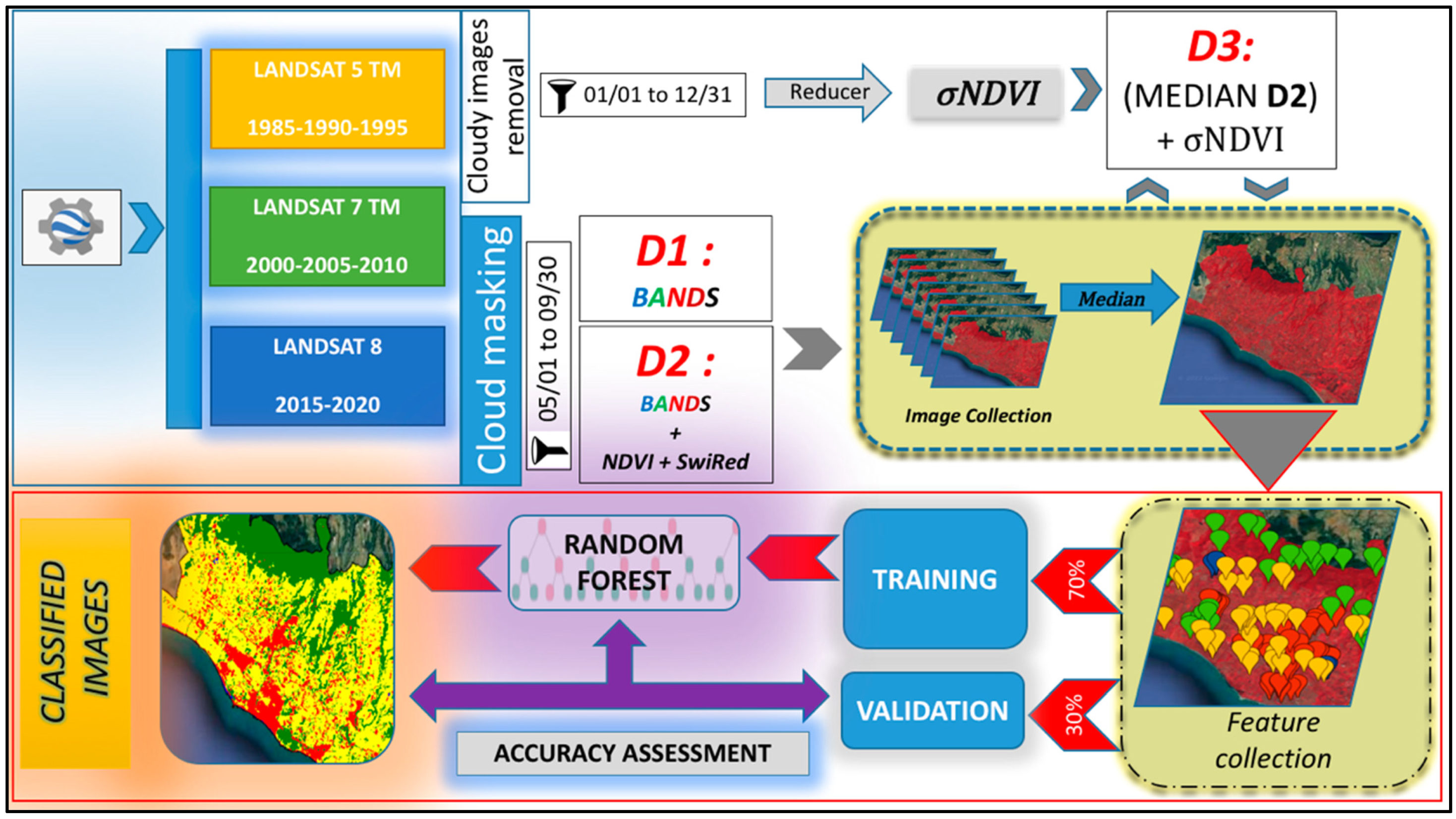
2.2. Satellite Data
2.3. Classification
- Urban: artificial surfaces of various types, tiles and sheet metal roofs, asphalt roads, greenhouses, concrete, etc.;
- Woodland: area with dense and tall vegetation;
- Permeable Areas: non-impervious surface, bare soil, agricultural areas subjected to cyclical tillage, sparsely vegetated permeable areas, orchards, and seasonal or permanent crops. Considering the purposes of the present study, which focused on urban expansion, it was chosen to enclose all of those permeable areas that were purely agricultural, grazing lands, and wasteland in a single category;
- Water Bodies: reservoirs and rivers.
2.4. Accuracy Assessment
2.5. Land Cover Change (LCc) Analysis
3. Results
3.1. Model Accuracies
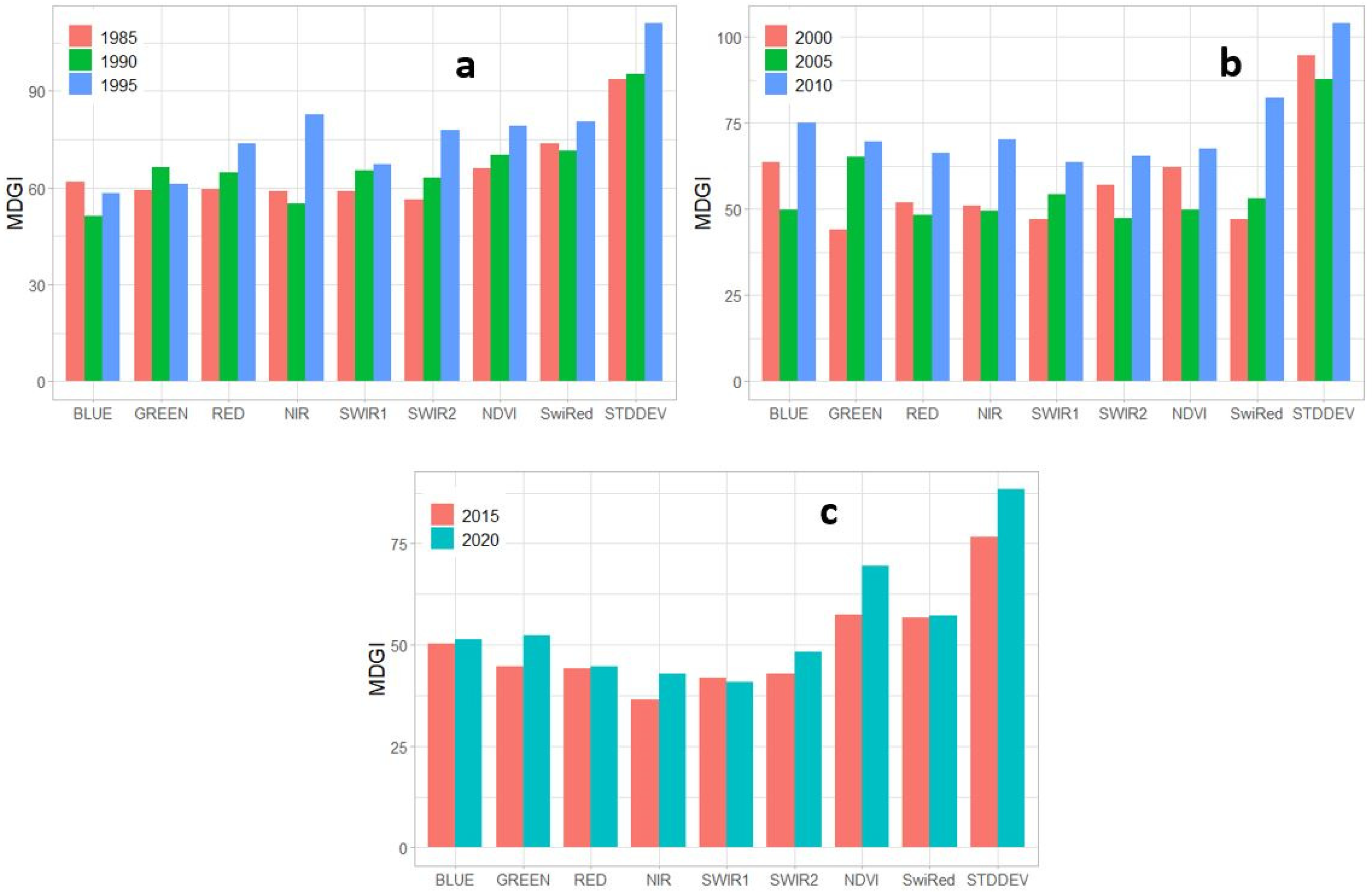
3.2. RF Performance
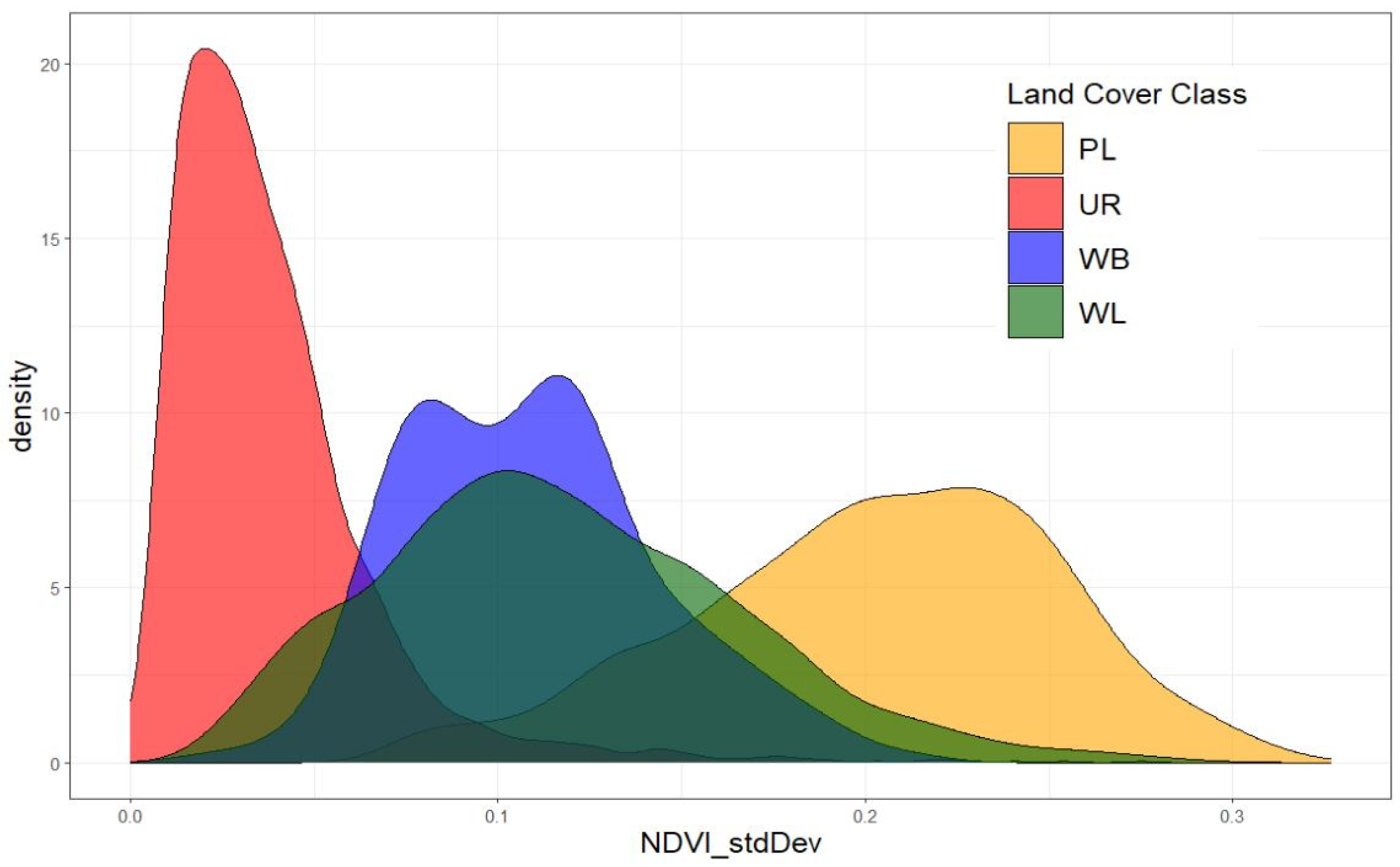
3.3. NDVI Standard Deviation
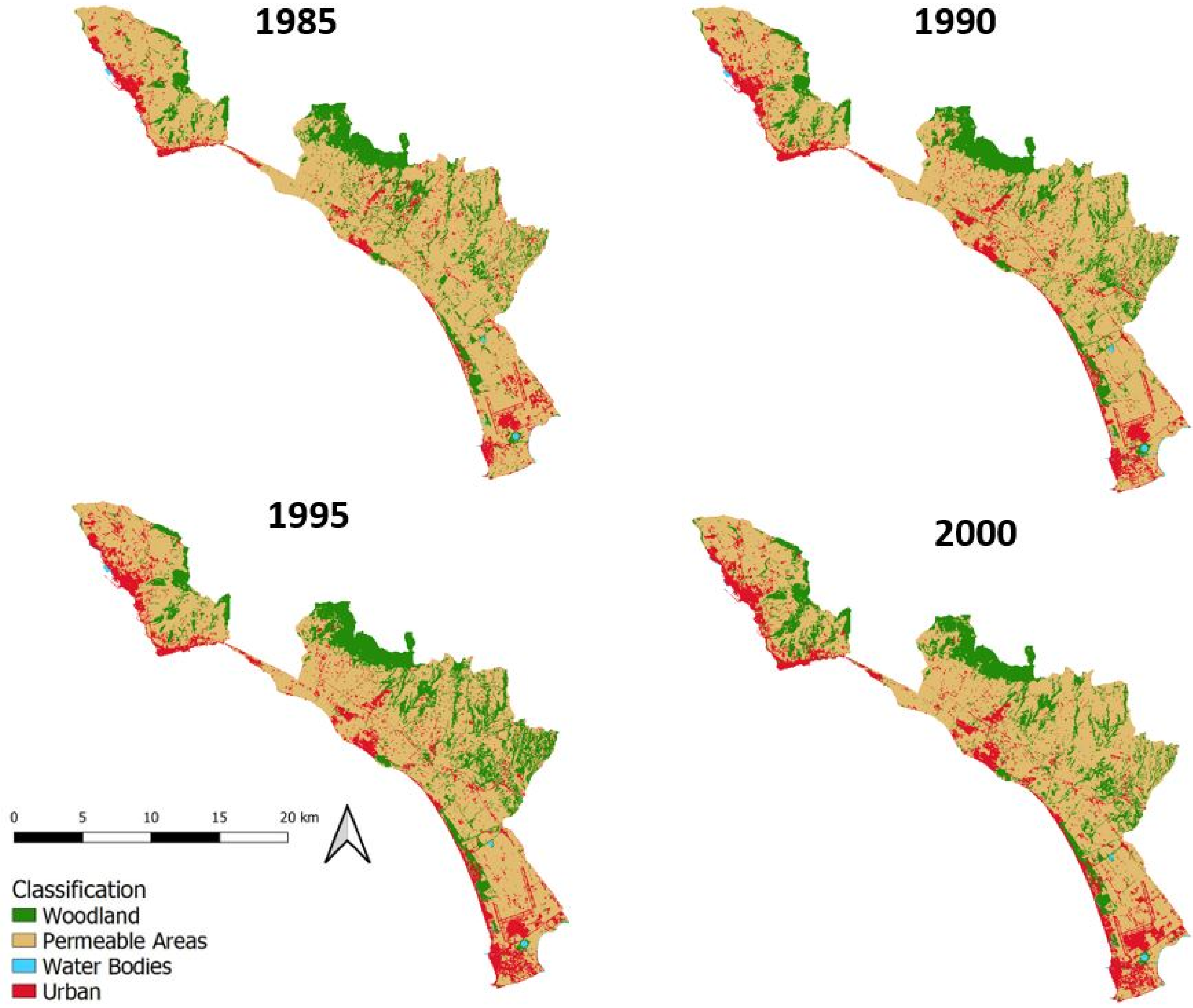
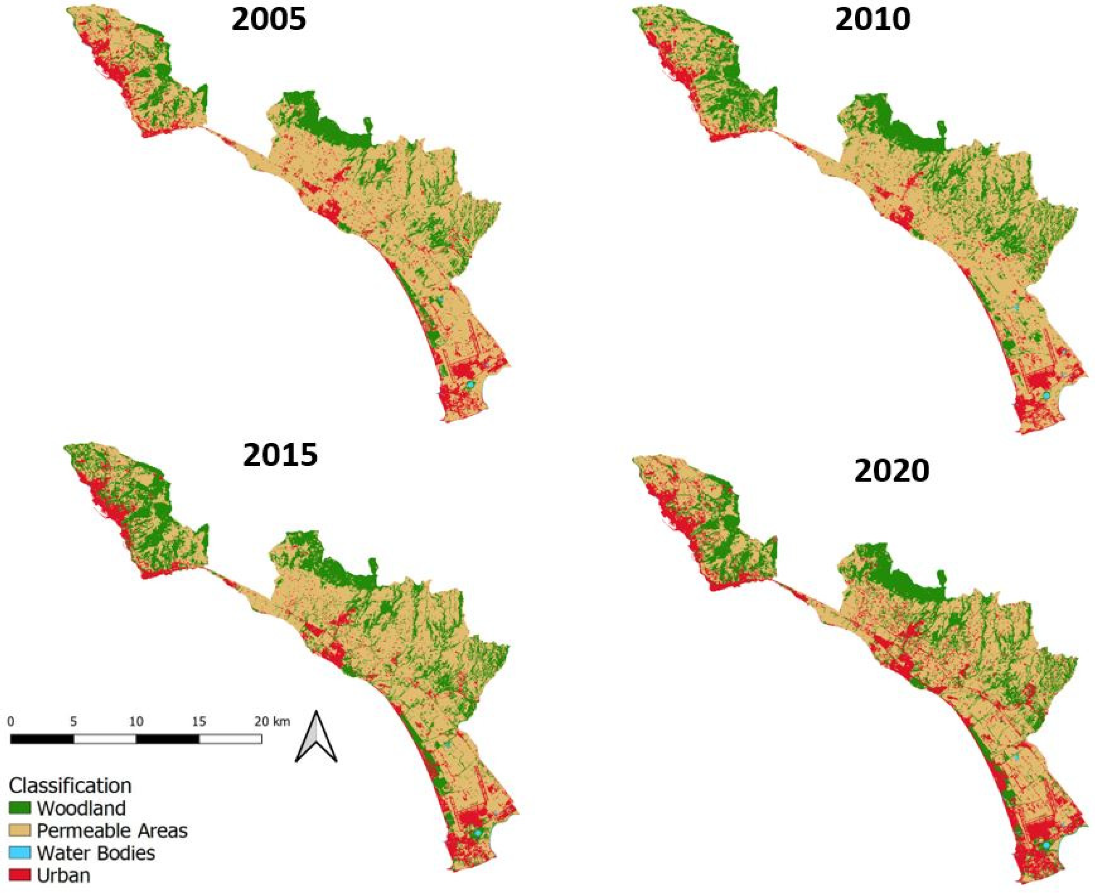
3.4. Classification
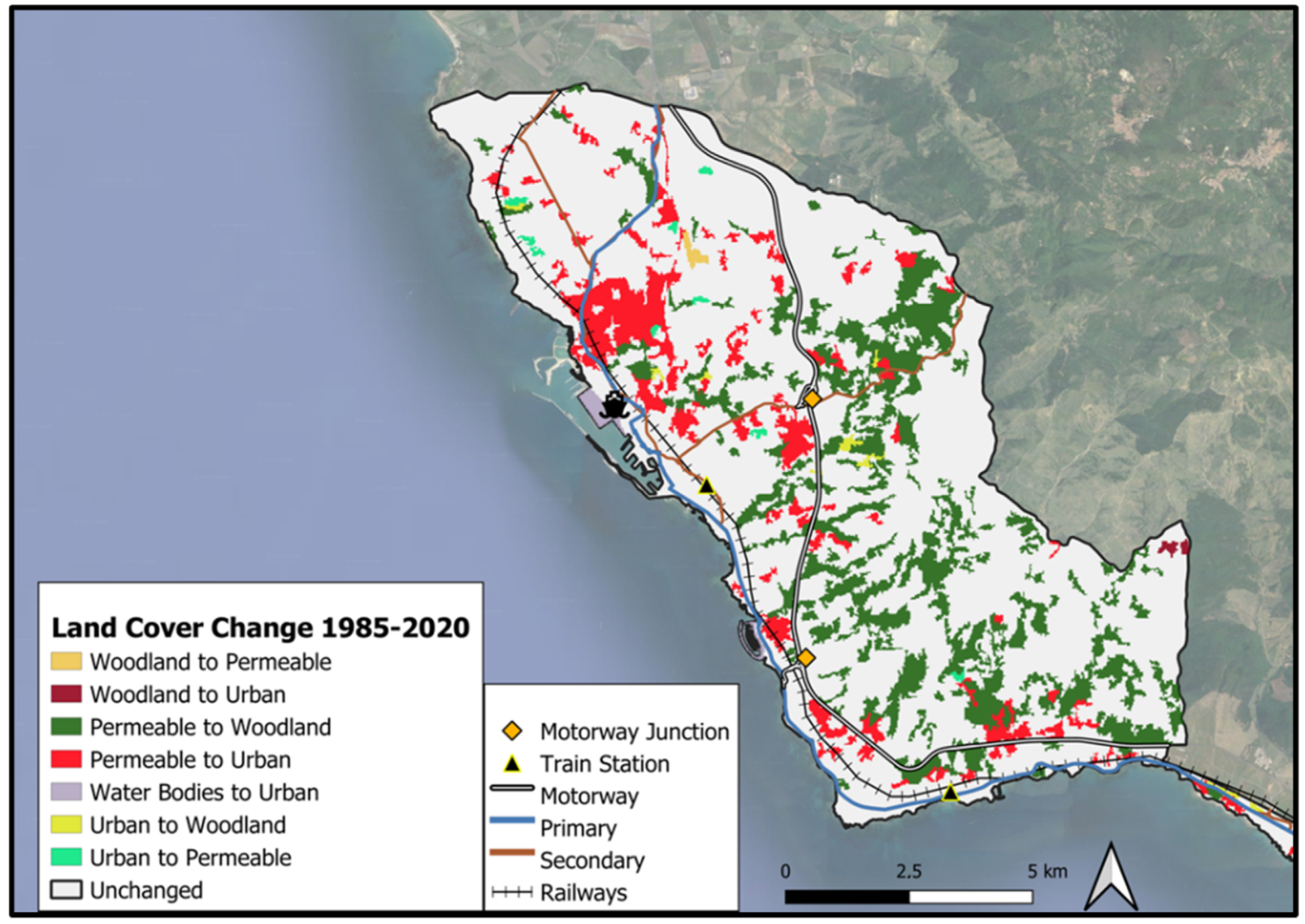
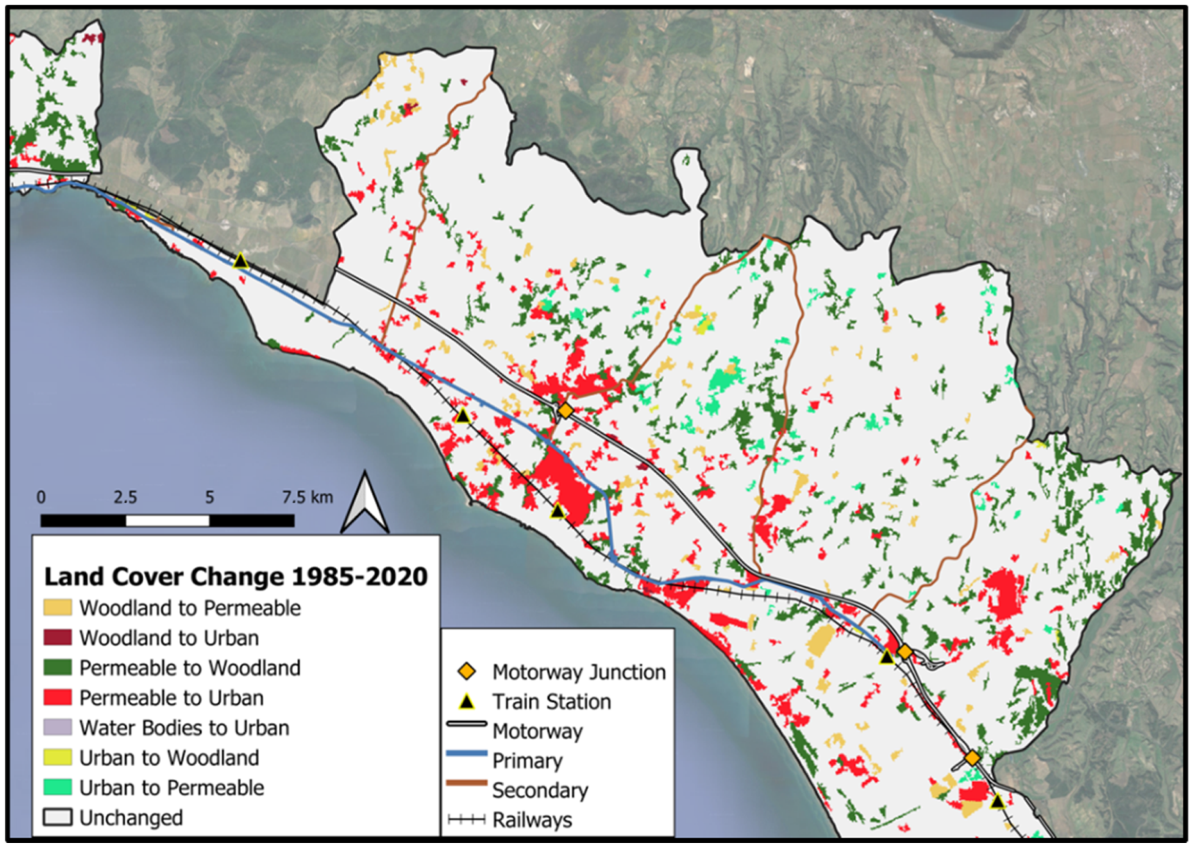
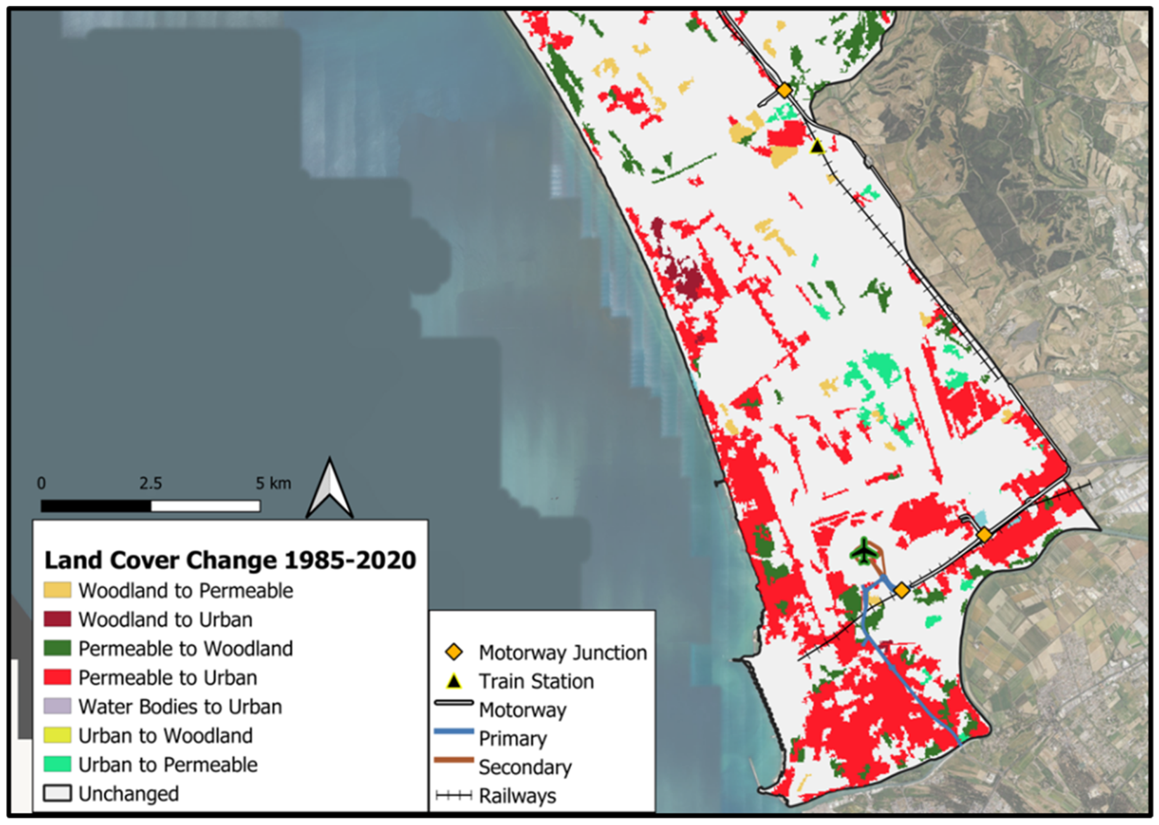
3.5. Land Cover Change 1985 ÷ 2020
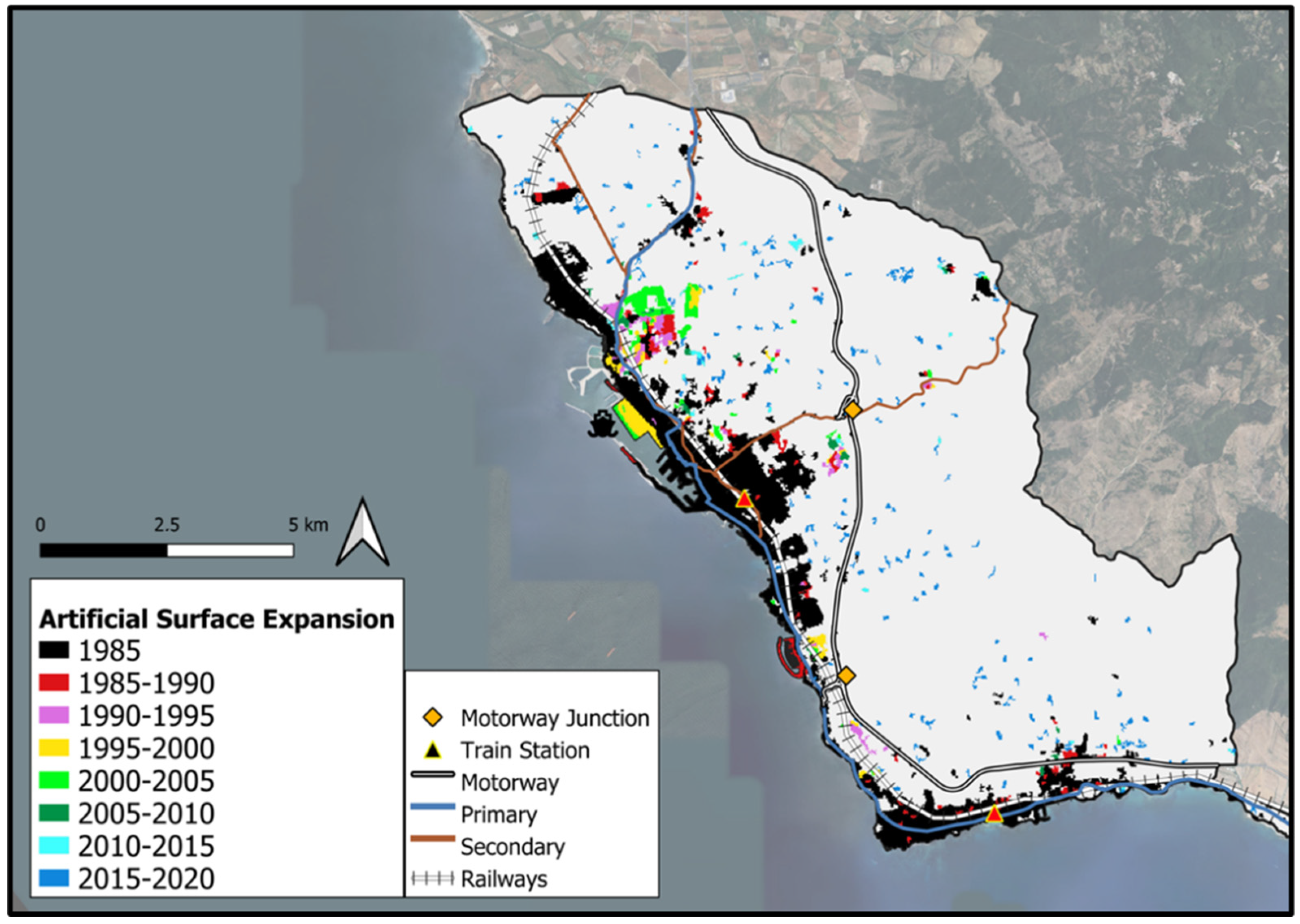
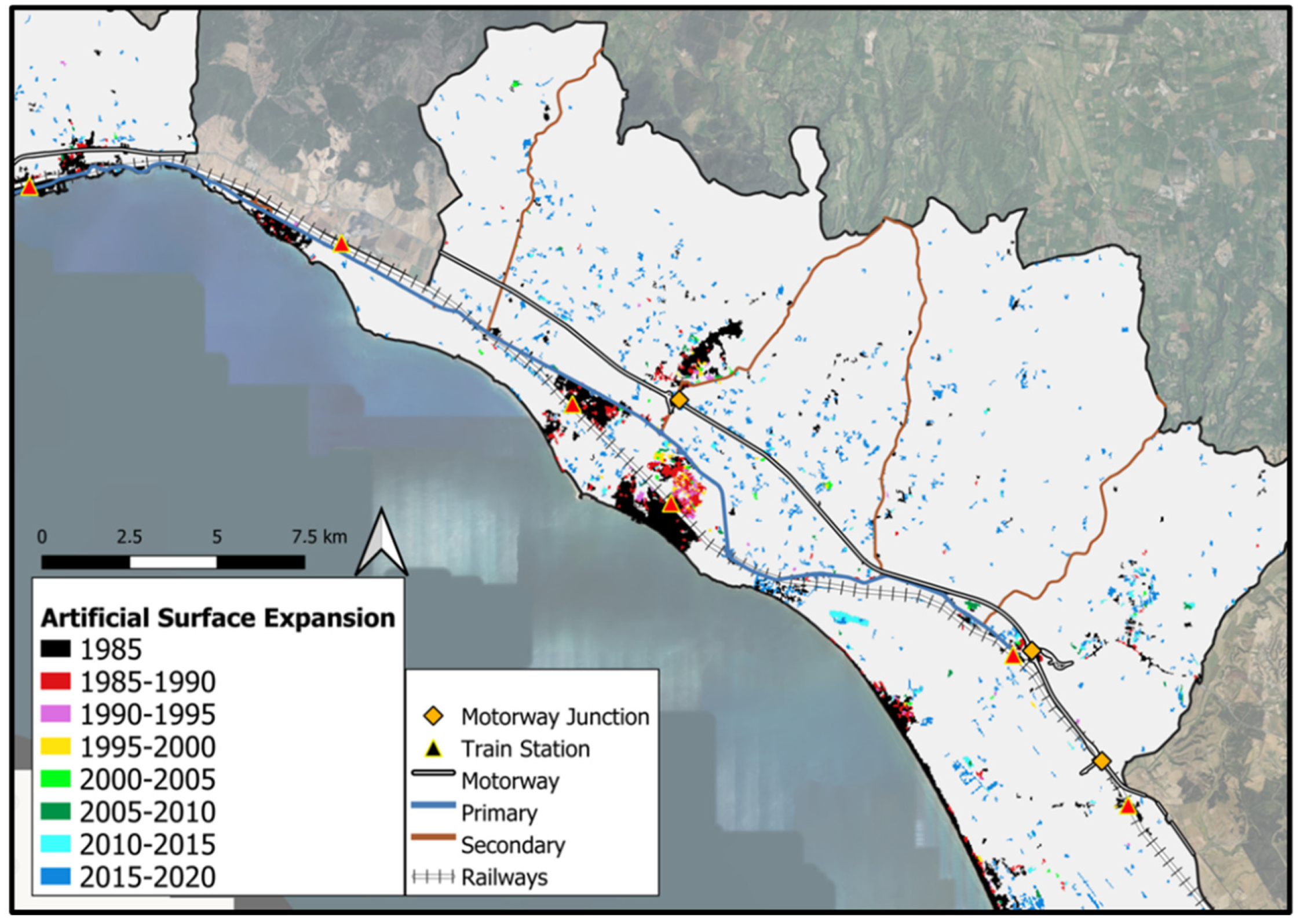
3.6. Spatio-Temporal Urban Expansion
4. Discussions
5. Conclusions
Author Contributions
Funding
Data Availability Statement
Acknowledgments
Conflicts of Interest
References
- Pandey, P.C.; Koutsias, N.; Petropoulos, G.P.; Srivastava, P.K.; Ben Dor, E. Land use/land cover in view of earth observation: Data sources, input dimensions, and classifiers—A review of the state of the art. Geocarto Int. 2021, 36, 957–988. [Google Scholar] [CrossRef]
- Modica, G.; Praticò, S.; Di Fazio, S. Abandonment of traditional terraced landscape: A change detection approach (a case study in Costa Viola, Calabria, Italy). Land Degrad. Dev. 2017, 28, 2608–2622. [Google Scholar] [CrossRef]
- Modica, G.; Vizzari, M.; Pollino, M.; Fichera, C.R.; Zoccali, P.; Di Fazio, S. Spatio-temporal analysis of the urban–rural gradient structure: An application in a Mediterranean mountainous landscape (Serra San Bruno, Italy). Earth Syst. Dyn. 2012, 3, 263–279. [Google Scholar] [CrossRef]
- Pollino, M.; Lodato, F.; Colonna, N. Spatio-Temporal Dynamics of Urban and Natural Areas in the Northern Littoral Zone of Rome. In Computational Science and Its Applications—ICCSA 2020; ICCSA 2020 Lecture Notes in Computer Science; Springer: Cham, Switzerland, 2020; Volume 12253, pp. 567–575. [Google Scholar]
- Calzolari, C.; Tarocco, P.; Lombardo, N.; Marchi, N.; Ungaro, F. Assessing soil ecosystem services in urban and peri-urban areas: From urban soils survey to providing support tool for urban planning. Land Use Policy 2020, 99, 105037. [Google Scholar] [CrossRef]
- Available online: https://www.un.org/development/desa/publications/2018-revision-of-world-urbanization-prospects.html (accessed on 18 March 2023).
- Reba, M.; Seto, K.C. A systematic review and assessment of algorithms to detect, characterize, and monitor urban land change. Remote Sens. Environ. 2020, 242, 111739. [Google Scholar] [CrossRef]
- Fichera, C.R.; Modica, G.; Pollino, M. Land Cover classification and change-detection analysis using multi-temporal remote sensed imagery and landscape metrics. Eur. J. Remote Sens. 2012, 45, 1–18. [Google Scholar] [CrossRef]
- Gómez, C.; White, J.C.; Wulder, M.A. Optical remotely sensed time series data for land cover classification: A review. ISPRS J. Photogramm. Remote Sens. 2016, 116, 55–72. [Google Scholar] [CrossRef]
- De Luca, G.; Silva, J.M.N.; Di Fazio, S.; Modica, G. Integrated use of Sentinel-1 and Sentinel-2 data and open-source machine learning algorithms for land cover mapping in a Mediterranean region. Eur. J. Remote Sens. 2022, 55, 52–70. [Google Scholar] [CrossRef]
- Sexton, J.O.; Song, X.-P.; Huang, C.; Channan, S.; Baker, M.E.; Townshend, J.R. Urban growth of the Washington, D.C.–Baltimore, MD metropolitan region from 1984 to 2010 by annual, Landsat-based estimates of impervious cover. Remote Sens. Environ. 2013, 129, 42–53. [Google Scholar] [CrossRef]
- Hu, H.; Ban, Y. Unsupervised Change Detection in Multitemporal SAR Images Over Large Urban Areas. IEEE J. Sel. Top. Appl. Earth Obs. Remote Sens. 2014, 7, 3248–3261. [Google Scholar] [CrossRef]
- Appiah, D.; Schröder, D.; Forkuo, E.; Bugri, J. Application of Geo-Information Techniques in Land Use and Land Cover Change Analysis in a Peri-Urban District of Ghana. ISPRS Int. J. Geo-Inf. 2015, 4, 1265–1289. [Google Scholar] [CrossRef]
- Christensen, P.; McCord, G.C. Geographic determinants of China’s urbanization. Reg. Sci. Urban Econ. 2016, 59, 90–102. [Google Scholar] [CrossRef]
- Mertes, C.M.; Schneider, A.; Sulla-Menashe, D.; Tatem, A.J.; Tan, B. Detecting change in urban areas at continental scales with MODIS data. Remote Sens. Environ. 2015, 158, 331–347. [Google Scholar] [CrossRef]
- Zhou, Y.; Smith, S.J.; Zhao, K.; Imhoff, M.; Thomson, A.; Bond-Lamberty, B.; Asrar, G.R.; Zhang, X.; He, C.; Elvidge, C.D. A global map of urban extent from nightlights. Environ. Res Lett. 2015, 10, 054011. [Google Scholar] [CrossRef]
- Mao, W.; Lu, D.; Hou, L.; Liu, X.; Yue, W. Comparison of Machine-Learning Methods for Urban Land-Use Mapping in Hangzhou City, China. Remote Sens. 2020, 12, 2817. [Google Scholar] [CrossRef]
- Huang, B.; Zhao, B.; Song, Y. Urban land-use mapping using a deep convolutional neural network with high spatial resolution multispectral remote sensing imagery. Remote Sens. Environ. 2018, 214, 73–86. [Google Scholar] [CrossRef]
- Gbanie, S.; Griffin, A.; Thornton, A. Impacts on the Urban Environment: Land Cover Change Trajectories and Landscape Fragmentation in Post-War Western Area, Sierra Leone. Remote Sens. 2018, 10, 129. [Google Scholar] [CrossRef]
- Reynolds, R.; Liang, L.; Li, X.; Dennis, J. Monitoring Annual Urban Changes in a Rapidly Growing Portion of Northwest Arkansas with a 20-Year Landsat Record. Remote Sens. 2017, 9, 71. [Google Scholar] [CrossRef]
- Samal, D.R.; Gedam, S.S. Monitoring land use changes associated with urbanization: An object based image analysis approach. Eur. J. Remote Sens. 2015, 48, 85–99. [Google Scholar] [CrossRef]
- Pandey, B.; Zhang, Q.; Seto, K.C. Time series analysis of satellite data to characterize multiple land use transitions: A case study of urban growth and agricultural land loss in India. J. Land Use Sci. 2018, 13, 221–237. [Google Scholar] [CrossRef]
- Mahmoud, H.; Divigalpitiya, P. Spatiotemporal variation analysis of urban land expansion in the establishment of new communities in Upper Egypt: A case study of New Asyut city. Egypt J. Remote Sens. Sp. Sci. 2019, 22, 59–66. [Google Scholar] [CrossRef]
- Chai, B.; Seto, K.C. Conceptualizing and characterizing micro-urbanization: A new perspective applied to Africa. Landsc. Urban Plan. 2019, 190, 103595. [Google Scholar] [CrossRef]
- Ma, Y.; Wu, H.; Wang, L.; Huang, B.; Ranjan, R.; Zomaya, A.; Jie, W. Remote sensing big data computing: Challenges and opportunities. Future Gener. Comput. Syst. 2015, 51, 47–60. [Google Scholar] [CrossRef]
- Gorelick, N.; Hancher, M.; Dixon, M.; Ilyushchenko, S.; Thau, D.; Moore, R. Google Earth Engine: Planetary-scale geospatial analysis for everyone. Remote Sens. Environ. 2017, 202, 18–27. [Google Scholar] [CrossRef]
- Schmitt, M.; Hughes, L.H.; Qiu, C.; Zhu, X.X. Aggregating Cloud-Free Sentinel-2 Images with Google Earth Engine. ISPRS Ann. Photogramm. Remote Sens. Spat. Inf. Sci. 2019, IV-2/W7, 145–152. [Google Scholar] [CrossRef]
- Belcore, E.; Piras, M.; Wozniak, E. Specific Alpine Environment Land Cover Classification Methodology: Google Earth Engine Processing for Sentinel-2 Data. Int. Arch. Photogramm. Remote Sens. Spat. Inf. Sci. 2020, XLIII-B3-2, 663–670. [Google Scholar] [CrossRef]
- Kumar, L.; Mutanga, O. Google Earth Engine Applications Since Inception: Usage, Trends, and Potential. Remote Sens. 2018, 10, 1509. [Google Scholar] [CrossRef]
- Tamiminia, H.; Salehi, B.; Mahdianpari, M.; Quackenbush, L.; Adeli, S.; Brisco, B. Google Earth Engine for geo-big data applications: A meta-analysis and systematic review. ISPRS J. Photogramm. Remote Sens. 2020, 164, 152–170. [Google Scholar] [CrossRef]
- Yang, L.; Driscol, J.; Sarigai, S.; Wu, Q.; Chen, H.; Lippitt, C.D. Google Earth Engine and Artificial Intelligence (AI): A Comprehensive Review. Remote Sens. 2022, 14, 3253. [Google Scholar] [CrossRef]
- Fattore, C.; Abate, N.; Faridani, F.; Masini, N.; Lasaponara, R. Google Earth Engine as Multi-Sensor Open-Source Tool for Supporting the Preservation of Archaeological Areas: The Case Study of Flood and Fire Mapping in Metaponto, Italy. Sensors 2021, 21, 1791. [Google Scholar] [CrossRef] [PubMed]
- Lasaponara, R.; Abate, N.; Masini, N. On the Use of Google Earth Engine and Sentinel Data to Detect “Lost” Sections of Ancient Roads. The Case of Via Appia. IEEE Geosci. Remote Sens. Lett. 2022, 19, 3001605. [Google Scholar] [CrossRef]
- Danese, M.; Gioia, D.; Biscione, M. Integrated Methods for Cultural Heritage Risk Assessment: Google Earth Engine, Spatial Analysis, Machine Learning. In Proceedings of the Computational Science and Its Applications–ICCSA 2021: 21st International Conference, Cagliari, Italy, 13–16 September 2021; pp. 605–619. [Google Scholar]
- Clemente, J.P.; Fontanelli, G.; Ovando, G.G.; Roa, Y.L.B.; Lapini, A.; Santi, E. Google Earth Engine: Application of Algorithms for Remote Sensing of Crops in Tuscany (Italy). Int. Arch. Photogramm. Remote Sens. Spat. Inf. Sci. 2020, XLII-3/W12, 291–296. [Google Scholar] [CrossRef]
- Balestra, M.; Chiappini, S.; Malinverni, E.S.; Galli, A.; Marcheggiani, E. A Machine Learning Approach for Mapping Forest Categories: An Application of Google Earth Engine for the Case Study of Monte Sant’Angelo, Central Italy. In Proceedings of the Computational Science and Its Applications–ICCSA 2021: 21st International Conference, Cagliari, Italy, 13–16 September 2021; pp. 155–168. [Google Scholar]
- Pérez-Cutillas, P.; Pérez-Navarro, A.; Conesa-García, C.; Zema, D.A.; Amado-Álvarez, J.P. What is going on within google earth engine? A systematic review and meta-analysis. Remote Sens. Appl. Soc. Environ. 2023, 29, 100907. [Google Scholar] [CrossRef]
- Goldblatt, R.; You, W.; Hanson, G.; Khandelwal, A. Detecting the Boundaries of Urban Areas in India: A Dataset for Pixel-Based Image Classification in Google Earth Engine. Remote Sens. 2016, 8, 634. [Google Scholar] [CrossRef]
- Sengupta, D.; Chen, R.; Meadows, M.E.; Choi, Y.R.; Banerjee, A.; Zilong, X. Mapping Trajectories of Coastal Land Reclamation in Nine Deltaic Megacities using Google Earth Engine. Remote Sens. 2019, 11, 2621. [Google Scholar] [CrossRef]
- Zhang, Z.; Wei, M.; Pu, D.; He, G.; Wang, G.; Long, T. Assessment of Annual Composite Images Obtained by Google Earth Engine for Urban Areas Mapping Using Random Forest. Remote Sens. 2021, 13, 748. [Google Scholar] [CrossRef]
- Carneiro, E.; Lopes, W.; Espindola, G. Urban Land Mapping Based on Remote Sensing Time Series in the Google Earth Engine Platform: A Case Study of the Teresina-Timon Conurbation Area in Brazil. Remote Sens. 2021, 13, 1338. [Google Scholar] [CrossRef]
- Phan, T.N.; Kuch, V.; Lehnert, L.W. Land Cover Classification using Google Earth Engine and Random Forest Classifier—The Role of Image Composition. Remote Sens. 2020, 12, 2411. [Google Scholar] [CrossRef]
- Solano, F.; Praticò, S.; Piovesan, G.; Chiarucci, A.; Argentieri, A.; Modica, G. Characterising historical transformation trajectories of the forest landscape in Rome’s Metropolitan area (Italy) for effective planning of sustainability goals. Land Degrad. Dev. 2021, 32, 4708–4726. [Google Scholar] [CrossRef]
- Bozzano, F.; Esposito, C.; Mazzanti, P.; Patti, M.; Scancella, S. Imaging Multi-Age Construction Settlement Behaviour by Advanced SAR Interferometry. Remote Sens. 2018, 10, 1137. [Google Scholar] [CrossRef]
- Della Ventura, G.; Patané, A. Le miniere dei Monti della Tolfa-Allumiere (Roma). In I siti della memoria geologica nel territorio del Lazio. Memorie Descrittive della Carta Geologica d’Italia; Pantaloni, M., Console, F., Argentieri, A., Mantero, D., Eds.; Servizio Geologico d’Italia—ISPRA: Rome, Italy, 2020; Volume 106, 328p, pp. 23–32. ISBN 978-88-9311-0815. [Google Scholar]
- Pietro, R.; Azzella, M.; Facioni, L. The Forest Vegetation of the Tolfa-Ceriti Mountains (Northern Latium—Central Italy). Hacquetia 2010, 9, 91–150. [Google Scholar] [CrossRef]
- Rouse, J.W.; Hass, R.H.; Schell, J.A.; Deering, D.W. Monitoring vegetation systems in the great plains with ERTS. Third Earth Resour. Technol. Satell. Symp. 1973, 1, 309–317. [Google Scholar]
- Capolupo, A.; Monterisi, C.; Tarantino, E. Landsat Images Classification Algorithm (LICA) to automatically extract land cover information in Google Earth Engine environment. Remote Sens. 2020, 12, 1201. [Google Scholar] [CrossRef]
- Jones, H.G.; Vaughan, R.A. Remote Sensing of Vegetation: Principles, Techniques, and Applications, 1st ed.; Oxford University Press: Oxford, UK, 2010; p. 353. [Google Scholar]
- Javed, A.; Cheng, Q.; Peng, H.; Altan, O.; Li, Y.; Ara, I.; Huq, E.; Ali, Y.; Saleem, N. Review of Spectral Indices for Urban Remote Sensing. Photogramm. Eng. Remote Sens. 2021, 87, 513–524. [Google Scholar] [CrossRef]
- Tassi, A.; Gigante, D.; Modica, G.; Di Martino, L.; Vizzari, M. Pixel- vs. Object-Based Landsat 8 Data Classification in Google Earth Engine Using Random Forest: The Case Study of Maiella National Park. Remote Sens. 2021, 13, 2299. [Google Scholar] [CrossRef]
- Nguyen, Q.H.; Ly, H.-B.; Ho, L.S.; Al-Ansari, N.; Le, H.V.; Tran, V.Q.; Prakash, I.; Pham, B.T. Influence of Data Splitting on Performance of Machine Learning Models in Prediction of Shear Strength of Soil. Math. Probl. Eng. 2021, 2021, 1–15. [Google Scholar] [CrossRef]
- Breiman, L. Random forests. Mach. Learn. 2001, 45, 5–32. [Google Scholar] [CrossRef]
- Praticò, S.; Solano, F.; Di Fazio, S.; Modica, G. Machine Learning Classification of Mediterranean Forest Habitats in Google Earth Engine Based on Seasonal Sentinel-2 Time-Series and Input Image Composition Optimisation. Remote Sens. 2021, 13, 586. [Google Scholar] [CrossRef]
- Li, X.; Chen, W.; Cheng, X.; Wang, L. A Comparison of Machine Learning Algorithms for Mapping of Complex Surface-Mined and Agricultural Landscapes Using ZiYuan-3 Stereo Satellite Imagery. Remote Sens. 2016, 8, 514. [Google Scholar] [CrossRef]
- Cutler, D.R.; Edwards, T.C.; Beard, K.H.; Cutler, A.; Hess, K.T.; Gibson, J.; Lawler, J.J. Random Forests for Classification in Ecology. Ecology 2007, 88, 2783–2792. [Google Scholar] [CrossRef] [PubMed]
- Li, Z.; Xin, X.; Tang, H.; Yang, F.; Chen, B.; Zhang, B. Estimating grassland LAI using the Random Forests approach and Landsat imagery in the meadow steppe of Hulunber, China. J. Integr. Agric. 2017, 16, 286–297. [Google Scholar] [CrossRef]
- Han, H.; Guo, X.; Yu, H. Variable selection using Mean Decrease Accuracy and Mean Decrease Gini based on Random Forest. In Proceedings of the 2016 7th IEEE International Conference on Software Engineering and Service Science (ICSESS), Beijing, China, 26–28 August 2016; IEEE: Piscataway, NJ, USA, 2016; pp. 219–224. [Google Scholar]
- Mellor, A.; Haywood, A.; Stone, C.; Jones, S. The Performance of Random Forests in an Operational Setting for Large Area Sclerophyll Forest Classification. Remote Sens. 2013, 5, 2838–2856. [Google Scholar] [CrossRef]
- Congalton, R.G.; Green, K. Assessing the Accuracy of Remotely Sensed Data [Internet]; CRC Press: Boca Raton, FL, USA, 2019. [Google Scholar]
- Story, M.; Congalton, R.G. Remote Sensing Brief Accuracy Assessment: A User’s Perspective. Photogramm. Eng. Remote Sens. 1986, 52, 397–399. [Google Scholar]
- Cohen, J. A Coefficient of Agreement for Nominal Scales. Educ. Psychol. Meas. 1960, 20, 37–46. [Google Scholar] [CrossRef]
- Momeni, R.; Aplin, P.; Boyd, D. Mapping Complex Urban Land Cover from Spaceborne Imagery: The Influence of Spatial Resolution, Spectral Band Set and Classification Approach. Remote Sens. 2016, 8, 88. [Google Scholar] [CrossRef]
- McNemar, Q. Note on the sampling error of the difference between correlated proportions or percentages. Psychometrika 1947, 12, 153–157. [Google Scholar] [CrossRef]
- Modica, G.; De Luca, G.; Messina, G.; Praticò, S. Comparison and assessment of different object-based classifications using machine learning algorithms and UAVs multispectral imagery: A case study in a citrus orchard and an onion crop. Eur. J. Remote Sens. 2021, 54, 431–460. [Google Scholar] [CrossRef]
- Matarira, D.; Mutanga, O.; Naidu, M. Google Earth Engine for Informal Settlement Mapping: A Random Forest Classification Using Spectral and Textural Information. Remote Sens. 2022, 14, 5130. [Google Scholar] [CrossRef]
- Cipriani, L.E.; Ferri, S.; Lami, G.; Pranzini, E. Human Impact on Shoreline Evolution Along the Follonica Gulf (Southern Tuscany): How Tourism May Kill the Goose that Lays the Golden Eggs. J. Coast. Res. 2011, 61, 290–294. [Google Scholar] [CrossRef]
- Fuerst-Bjeliš, B.; Durbešić, A. Littoralization and behind: Environmental Change in Mediterranean Croatia. In The Overarching Issues of the European Space/Strategies for Spatial (Re)Planning Based on Innovation, Sustainability and Change; Pina, H., Martins, F., Ferreira, C., Eds.; Fundação Universidade Do Porto—Faculdade de Letras da Universidade do Porto: Porto, Portugal, 2013; pp. 136–147. [Google Scholar] [CrossRef]
- Manganelli, B.; Murgante, B. The Dynamics of Urban Land Rent in Italian Regional Capital Cities. Land 2017, 6, 54. [Google Scholar] [CrossRef]
- Salvati, L.; Sabbi, A. Exploring long-term land cover changes in an urban region of southern Europe. Int. J. Sustain. Dev. World Ecol. 2011, 18, 273–282. [Google Scholar] [CrossRef]
- Biasi, R.; Colantoni, A.; Ferrara, C.; Ranalli, F.; Salvati, L. In-between sprawl and fires: Long-term forest expansion and settlement dynamics at the wildland–urban interface in Rome, Italy. Int. J. Sustain. Dev. World Ecol. 2015, 22, 467–475. [Google Scholar] [CrossRef]
- De Felice, P.; Grillotti Di Giacomo, M.G. Land Grabbing e Land Concentration. I Predatori Della Terra Tra Neocolonialismo e Crisi Migratorie; Franco Angeli: Milan, Italy, 2018. [Google Scholar]
- Lelo, K. Agro Romano: Un territorio in trasformazione. In Roma Moderna e Contemporanea; Università Toma tre—CROMA: Roma, Italy, 2016; pp. 9–48. [Google Scholar] [CrossRef]
- De Felice, P.; Lodato, F. La tenuta di Zambra nell’agro romano oltre la Convenzione Europea del Paesaggio. Un’analisi geografica a scala locale. In Oltre la Convenzione Pensare, Studiare, Costruire il Paesaggio Vent’anni Dopo; Società di Studi Geografici: Firenze, Italy, 2020; pp. 702–721. [Google Scholar]
- Salvati, L. “A Chronicle of a Death Foretold”: Urban Expansion and Land Consumption in Rome, Italy. Eur. Plan. Stud. 2013, 21, 1176–1188. [Google Scholar] [CrossRef]
- Praticò, S.; Solano, F.; Di Fazio, S.; Modica, G. A Multitemporal Fragmentation-Based Approach for a Dynamics Analysis of Agricultural Terraced Systems: The Case Study of Costa Viola Landscape (Southern Italy). Land 2022, 11, 482. [Google Scholar] [CrossRef]
- Modica, G.; Merlino, A.; Solano, F.; Mercurio, R. An index for the assessment of degraded Mediterranean forest ecosystems. For. Syst. 2015, 24, e037. [Google Scholar] [CrossRef]
- Caneva, G.; Benelli, F.; Bartoli, F.; Cicinelli, E. Safeguarding natural and cultural heritage on Etruscan tombs (La Banditaccia, Cerveteri, Italy). Rend. Lincei Sci. Fis. Nat. 2018, 29, 891–907. [Google Scholar] [CrossRef]
- Pollino, M.; Modica, G. Free Web Mapping Tools to Characterise Landscape Dynamics and to Favour e-Participation. In Computational Science and Its Applications—ICCSA 2013. Lecture Notes In Computer Science; Murgante, B., Misra, S., Carlini, M., Torre, C.M., Nguyen, H.-Q., Taniar, D., Apduhan, B.O., Gervasi, O., Eds.; Springer: Berlin/Heidelberg, Germany, 2013; Volume 7973, pp. 566–581. [Google Scholar] [CrossRef]


| D1 | D2 | D3 | |
|---|---|---|---|
| 05/01 to 30/09 (median) | BLUE GREEN RED NIR SWIR1 SWIR2 | BLUE GREEN RED NIR SWIR1 SWIR2 | BLUE GREEN RED NIR SWIR1 SWIR2 |
| 05/01 to 30/09 (median) | NDVI SwiRed | NDVI SwiRed | |
| 01/01 to 31/12 | NDVI Standard Deviation | ||
| No. Variables | 6 | 8 | 9 |
| Year | 1985 | 1990 | 1995 | 2000 | 2005 | 2010 | 2015 | 2020 |
|---|---|---|---|---|---|---|---|---|
| 05/01 to 09/30 (D1–D2–D3) | 13 | 18 | 14 | 19 | 8 | 5 * | 28 | 22 |
| 01/01 to 12/31 (NDVI st. Dev.) | 11 | 17 | 16 | 19 | 12 | 6 | 25 | 36 |
| 1985 | Urban | Woodland | Permeable L. | Water B. | OA | K | |
| D1 | UA | 0.86 | 0.96 | 0.85 | 1 | 0.89 | 0.84 |
| PA | 0.87 | 0.95 | 0.85 | 1 | |||
| D2 | UA | 0.88 | 0.94 | 0.85 | 1 | 0.89 | 0.84 |
| PA | 0.85 | 0.98 | 0.85 | 1 | |||
| D3 | UA | 0.96 | 0.99 | 0.9 | 1 | 0.95 | 0.92 |
| PA | 0.91 | 0.98 | 0.95 | 1 | |||
| 1990 | Urban | Woodland | Permeable L. | Water B. | OA | K | |
| D1 | UA | 0.95 | 0.93 | 0.75 | 1 | 0.87 | 0.8 |
| PA | 0.87 | 0.81 | 0.91 | 1 | |||
| D2 | UA | 0.94 | 0.92 | 0.86 | 1 | 0.91 | 0.87 |
| PA | 0.95 | 0.92 | 0.86 | 0.8 | |||
| D3 | UA | 0.99 | 0.94 | 0.92 | 1 | 0.95 | 0.92 |
| PA | 0.99 | 0.94 | 0.92 | 1 | |||
| 1995 | Urban | Woodland | Permeable L. | Water B. | OA | K | |
| D1 | UA | 0.93 | 0.88 | 0.86 | 1 | 0.89 | 0.84 |
| PA | 0.97 | 0.9 | 0.8 | 0.83 | |||
| D2 | UA | 0.93 | 0.88 | 0.78 | 0.88 | 0.86 | 0.8 |
| PA | 0.9 | 0.86 | 0.83 | 0.8 | |||
| D3 | UA | 0.97 | 0.81 | 0.9 | 1 | 0.9 | 0.85 |
| PA | 0.95 | 0.95 | 0.85 | 0.8 | |||
| 2000 | Urban | Woodland | Permeable L. | Water B. | OA | K | |
| D1 | UA | 0.94 | 0.91 | 0.9 | 1 | 0.92 | 0.87 |
| PA | 0.91 | 0.99 | 0.85 | 1 | |||
| D2 | UA | 0.97 | 0.91 | 0.8 | 1 | 0.9 | 0.87 |
| PA | 0.85 | 0.91 | 0.89 | 1 | |||
| D3 | UA | 0.99 | 0.95 | 0.91 | 1 | 0.95 | 0.92 |
| PA | 0.95 | 0.96 | 0.94 | 1 | |||
| 2005 | Urban | Woodland | Permeable L. | Water B. | OA | K | |
| D1 | UA | 0.92 | 0.95 | 0.77 | 1 | 0.88 | 0.85 |
| PA | 0.85 | 0.89 | 0.89 | 1 | |||
| D2 | UA | 0.96 | 0.96 | 0.83 | 1 | 0.91 | 0.88 |
| PA | 0.88 | 0.9 | 0.94 | 1 | |||
| D3 | UA | 0.98 | 0.99 | 0.9 | 1 | 0.95 | 0.93 |
| PA | 0.95 | 0.92 | 0.98 | 1 | |||
| 2010 | Urban | Woodland | Permeable L. | Water B. | OA | K | |
| D1 | UA | 0.95 | 0.95 | 0.83 | 1 | 0.91 | 0.88 |
| PA | 0.91 | 0.87 | 0.92 | 1 | |||
| D2 | UA | 0.96 | 0.94 | 0.87 | 0.91 | 0.92 | 0.89 |
| PA | 0.91 | 0.93 | 0.91 | 1 | |||
| D3 | UA | 0.99 | 0.94 | 0.85 | 0.84 | 0.93 | 0.92 |
| PA | 0.98 | 0.89 | 0.9 | 1 | |||
| 2015 | Urban | Woodland | Permeable L. | Water B. | OA | K | |
| D1 | UA | 0.95 | 0.94 | 0.85 | 1 | 0.92 | 0.88 |
| PA | 0.9 | 0.96 | 0.86 | 1 | |||
| D2 | UA | 0.92 | 0.92 | 0.83 | 0.8 | 0.9 | 0.85 |
| PA | 0.9 | 0.94 | 0.82 | 1 | |||
| D3 | UA | 1 | 0.94 | 0.95 | 1 | 0.96 | 0.94 |
| PA | 0.99 | 0.96 | 0.93 | 1 | |||
| 2020 | Urban | Woodland | Permeable L. | Water B. | OA | K | |
| D1 | UA | 0.95 | 0.93 | 0.89 | 1 | 0.92 | 0.9 |
| PA | 0.93 | 0.93 | 0.9 | 1 | |||
| D2 | UA | 0.9 | 0.98 | 0.88 | 1 | 0.92 | 0.9 |
| PA | 0.93 | 0.95 | 0.9 | 0.87 | |||
| D3 | UA | 0.96 | 0.96 | 0.97 | 1 | 0.97 | 0.96 |
| PA | 1 | 0.98 | 0.95 | 0.85 | |||
| 1985 | 1990 | 1995 | 2000 | 2005 | 2010 | 2015 | 2020 | |
|---|---|---|---|---|---|---|---|---|
| D1-D2 | 0.96 | 0.19 | 0.36 | 0.43 | 0.21 | 0.77 | 0.5 | 1 |
| D1-D3 | <0.05 | <0.05 | 089 | 0.2 | <0.05 | 0.76 | <0.05 | <0.05 |
| D2-D3 | <0.05 | <0.05 | 0.2 | <0.05 | 0.05 | 0.76 | <0.05 | <0.05 |
| Year | 1985 | 1990 | 1995 | 2000 | 2005 | 2010 | 2015 | 2020 |
|---|---|---|---|---|---|---|---|---|
| D1 | 0.091 | 0.098 | 0.118 | 0.094 | 0.082 | 0.110 | 0.098 | 0.082 |
| D2 | 0.085 | 0.096 | 0.116 | 0.083 | 0.082 | 0.078 | 0.078 | 0.064 |
| D3 | 0.066 | 0.066 | 0.081 | 0.054 | 0.054 | 0.06 | 0.045 | 0.048 |
| Diff. | Lwr | Upr | p-Value | |
|---|---|---|---|---|
| UR-PL | −0.164 | −0.166 | −0.161 | 9.67 × 10⁻¹² |
| WB-PL | −0.093 | −0.100 | −0.086 | 9.67 × 10⁻¹² |
| WL-PL | −0.085 | −0.087 | −0.082 | 9.67 × 10⁻¹² |
| WB-UR | 0.070 | 0.063 | 0.077 | 9.67 × 10⁻¹² |
| WL-UR | 0.079 | 0.076 | 0.081 | 9.67 × 10⁻¹² |
| WL-WB | 0.008 | 0.001 | 0.015 | 0.078 |
| LC Transitions 1985–2020 | Urban | Permeable Areas | Woodland | Water Bodies |
|---|---|---|---|---|
| Urban | - | 11.5 | 1.2 | <0.5 |
| Permeable Areas | 67.4 | - | 70.4 | |
| Woodland | 2 | 11.9 | - | <0.5 |
| Water Bodies | 0.5 | <0.5 | <0.5 | - |
Disclaimer/Publisher’s Note: The statements, opinions and data contained in all publications are solely those of the individual author(s) and contributor(s) and not of MDPI and/or the editor(s). MDPI and/or the editor(s) disclaim responsibility for any injury to people or property resulting from any ideas, methods, instructions or products referred to in the content. |
© 2023 by the authors. Licensee MDPI, Basel, Switzerland. This article is an open access article distributed under the terms and conditions of the Creative Commons Attribution (CC BY) license (https://creativecommons.org/licenses/by/4.0/).
Share and Cite
Lodato, F.; Colonna, N.; Pennazza, G.; Praticò, S.; Santonico, M.; Vollero, L.; Pollino, M. Analysis of the Spatiotemporal Urban Expansion of the Rome Coastline through GEE and RF Algorithm, Using Landsat Imagery. ISPRS Int. J. Geo-Inf. 2023, 12, 141. https://doi.org/10.3390/ijgi12040141
Lodato F, Colonna N, Pennazza G, Praticò S, Santonico M, Vollero L, Pollino M. Analysis of the Spatiotemporal Urban Expansion of the Rome Coastline through GEE and RF Algorithm, Using Landsat Imagery. ISPRS International Journal of Geo-Information. 2023; 12(4):141. https://doi.org/10.3390/ijgi12040141
Chicago/Turabian StyleLodato, Francesco, Nicola Colonna, Giorgio Pennazza, Salvatore Praticò, Marco Santonico, Luca Vollero, and Maurizio Pollino. 2023. "Analysis of the Spatiotemporal Urban Expansion of the Rome Coastline through GEE and RF Algorithm, Using Landsat Imagery" ISPRS International Journal of Geo-Information 12, no. 4: 141. https://doi.org/10.3390/ijgi12040141
APA StyleLodato, F., Colonna, N., Pennazza, G., Praticò, S., Santonico, M., Vollero, L., & Pollino, M. (2023). Analysis of the Spatiotemporal Urban Expansion of the Rome Coastline through GEE and RF Algorithm, Using Landsat Imagery. ISPRS International Journal of Geo-Information, 12(4), 141. https://doi.org/10.3390/ijgi12040141