Abstract
Java’s Brantas River Basin (BRB) is an increasingly urbanized tropical watershed with significant economic and ecological importance; yet knowledge of its land-use changes dynamics and drivers as well as their importance have barely been explored. This is the case for many other tropical watersheds in Java, Indonesia and beyond. This study of the BRB (1) quantifies the land-use changes in the period 1995–2015, (2) determines the patterns of land-use changes during 1995–2015, and (3) identifies the potential drivers of land-use changes during 1995–2015. Findings show that from 1995 to 2015, major transitions from forest to shrubs (218 km2), forest to dryland agriculture (512 km2), and from agriculture to urban areas (1484 km2) were observed in the BRB. Responses from land-user questionnaires suggest that drivers include a wide range of economic, social, technological, and biophysical attributes. An agreement matrix provided insight about consistency and inconsistency in the drivers inferred from the Land Change Modeler and those inferred from questionnaires. Factors that contributed to inconsistencies include the limited representation of local land-use features in the spatial data sets and comprehensiveness of land-user questionnaires. Together the two approaches signify the heterogeneity and scale-dependence of the land-use change process.
1. Introduction
Land-use is widely considered as a primary parameter of environmental change from local to global scales and is increasingly included in environmental change assessments [1,2]. Changes in land-uses may impact upon hydrology [3], biodiversity, water saving measures [4], and disaster risk [5]. Rapid land-use changes have often been associated with uncontrollable urban growth [6], farm loss [7], and deforestation [8].
The triggers or factors that lead to land-use changes or influence the process of land-use change are commonly termed “drivers” [9]. Studies show a broad range of drivers [10], which can be broadly categorized into biophysical factors (e.g., climate, soil, and terrain) and anthropogenic factors (e.g., population, technology, policy, culture, and economy) [11,12,13,14,15]. These drivers may be direct, such as a growing population [16] and increasing market prices [17]. Some others can be more complex, such as institutional and cultural settings [18]. It is widely accepted that changes, planned or not, are principally the consequence of human decisions [19]. Anthropogenic factors usually exhibit a more immediate impact than natural factors [14]. Studies show that drivers might interact with each other [20], and operate on differing scales, namely institutional, temporal, and spatial scales [9].
Information on land-use changes and their associated drivers is important for understanding the likely condition of future land-use and outlining land management strategies [21,22]. Relationships among drivers can be complex, and therefore it may be difficult to identify and quantify the primary drivers operating in a particular landscape [23]. Approaches to quantifying the relationship between drivers and land-use changes include economic modeling, systems theory, and spatial modeling [9,14,24,25,26]. Some studies employ qualitative household-level surveys to understand what triggers land-use conversion [12,27,28]. While spatial modeling can provide insight about spatial variability of drivers at a regional scale, surveys can provide information about drivers at a land-user or household or local scale [14]. However, most studies have employed only one approach—either quantitative modeling or qualitative surveys [7,29,30,31,32].
Land-use change studies are commonly carried out at a watershed level due to the pivotal role of watershed land-use dynamics in water resource policy and planning. Such studies support understanding of how land-use change and its interaction with climate influence the watershed’s hydrological functioning [33,34]. This is exemplified by several studies, such as those on the impact of climatic variability and land-uses on water resources [35,36], and the impact of increasing urban sprawl on water quality [37,38]. From an Indonesian context, urban sprawl has been considered a major factor in land-use change due to rapid population growth and it brings multiple consequences from ecological to socio–economic, which in turn affect the sustainability of the region and become a major consideration in land-use policy making [39].
Indonesia is a primary example of a tropical nation that continues to undergo rapid land-use changes marked with high extents of forest loss (0.31–0.69 Mha in 2000–2010) [40], massive urbanization [7], and associated environmental problems such as groundwater springs drying up [41]. Yet, research to support comprehensive understanding of land-use change in Indonesia and its impacts has been limited, scattered, inconsistent, and mostly focused on forest assessment studies outside Java. Relevant research has been conducted on the influence of population in shaping Java’s land-uses [26], the role of policy in shaping Indonesian land-use [42], and quantification of forest loss in Sumatra [8]. However, research providing insight into the dynamics of land-use change, patterns, and drivers over different scales is lacking, especially in Java.
The period from 1995 to 2015 is marked by socio–economic and political reforms in major Indonesian sectors such as agriculture and economy and governance [43,44,45,46,47]. In particular, during 2004–2005 Indonesia underwent a major administrative power shift through the implementation of local autonomy, providing more authority for regional level decision making, and also saw the introduction of a new long-term development policy in East Java [48]. Many studies suggested that this new policy led to elevated deforestation, intensified urbanization, and agricultural decline [48,49,50,51,52]. The mid-point of this period, 2004–2005, was also considered globally as the turning point of global surface transition [52]. Similar results from local perspectives support this finding. During this period, intensified urbanization from agricultural conversion has been observed in China, resulting in consideration for ecological sustainability assessment [51,52]. Similarly, in Indonesia, the period 1995–2015 was marked by a major shift in deforestation for palm plantation [53], massive urban sprawl [39], and deterioration in watershed [54]. Land-use changes have also been linked to the climate change in this period. In Nepal, changes in climatic variability, despite insignificant, in this period have been observed that were considered partially due to changes in land-uses [55]. Massive landscape transformation as well as its global implications then apparently stimulated the necessity of land-use change studies [56].
This research was carried out to investigate land-use change drivers in the Brantas River Basin (BRB), a large tropical watershed in the island of Java, Indonesia. The BRB can be regarded as a typical tropical developing country watershed in the sense that land-use change is rapid due to varying factors related to the growing population and economic development [42]. While rapid socio–economic and ecological dynamics have been observed in BRB [41,57,58], empirical evidence on the type, patterns, and drivers of these dynamics is limited. This study therefore aims to contribute to understanding of inter-decadal land-use dynamics, patterns, and drivers in tropical and developing countries. As opposed to most land-use change studies, our study combines geospatial regional scale modeling with local-scale questionnaires [7,29,30,31,32]. Using the two complementary approaches aims to allow a high degree of confidence in identifying principal land-use drivers. The study specifically aims to (1) quantify the land-use changes in BRB, (2) determine the patterns of land-use change in BRB, and (3) identify the potential drivers of land-use changes in BRB during 1995–2015 using two approaches: geospatial modeling and questionnaires.
2. Materials and Methods
2.1. Study Area
The BRB, with an area of 11,832 km2, covers approximately 30% of the province of East Java (Figure 1). The basin (“basin” is the term typically used for a large watershed in Indonesia and so is adopted in this paper) is home to two major cities and 13 regencies. These 15 administrative boundaries have their own statistics with scattered data coverage. Most areas have their data starting from 2005, and 2005–2017 is the longest period where the 15 areas have the common and full coverage to district population level. The population grew from around 21 million in 2005 to 22.5 million in 2017, accounting for 54% of East Java’s population and 7.5% of Indonesia’s population. The information of population presented here is to provide an overview of the demography of Brantas watershed.
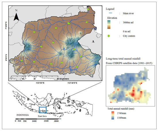
Figure 1.
(A) The BRB within East Java. The blue lines show the main river network. The green dots are the largest cities in the BRB. (B) BRB orientation in Indonesia.
Seven mountains create large topographical variability. Elevation ranges from sea-level to 3663 m above sea-level. Geology is heterogeneous, shaped by alluvial processes, lahar deposition, volcanic formation, and tuff depositions. The BRB exhibits a typical tropical monsoon climate with two distinct seasons: a dry season (April–October) and a wet season (November–March) [59]. Recorded long-term annual rainfall (1995–2015) ranges from an average of 2000 mm/year to nearly 3000 mm/year at high altitudes.
The BRB represents a mixed rural and urban society, with potentially competing land-uses. Growing urbanization and industrialization have led to encroachment on remaining forests, especially in the upper basin. Due to this, the ecosystem functions of the upper BRB have been considered poor for at least two decades [60] and there is an increasing number of environmental reports particularly related to the increasing challenges of drought, floods, eutrophication, water pollution, and sedimentation [41].
2.2. Land-Use Mapping Using Remote Sensing
The research approach is presented in Figure 2. The BRB spans four Landsat scenes each with 30 m resolution (Path:118/65–66 and Path:119/65–66). There are several considerations for the selection of Landsat images: the long coverage, richness in spectral variety [61,62], and suitability for mapping complex landscapes [63,64]. The years 1995, 2005, and 2015 were selected due to the quality of images during these years, the turning points of ecological and political conditions, and because the increasing environmental issues associated with land-use have increased since the 1990s [41,65]. The already georeferenced and atmospherically corrected surface reflectance products from NASA [66] were used to minimize atmospheric effect variations, which is especially important due to the use of multi-temporal and multi-tiled images [65,66,67,68]. To overcome difficulties in creating mosaics, we utilized a Google Earth Engine (GEE)-aided platform from Climate Engine [69]. We removed the clouds and shadowed pixels from analysis using the QA band in GEE and we utilized all available images after the cloud and shadow removal. For example, for 1995, we retrieved all images available from 1 January to 31 December 1995, and then applied the cloud and shadow removal. In each year we had 23 scenes for each path/row. We derived average images from all spectral bands of Landsat-7 for 1995 and 2005, and from Landsat-8 for 2015. The average image was selected instead of the median image because: (1) throughout the years of 1995, 2005, and 2015, there were no perceived extreme climatic events that might cause large differences in the reflectance of the objects, and the presence of outliers is negligible, (2) similarity in median and mean image histograms, and (3) deriving the median image is more computationally heavy [70]. Screening resulted in 16 to 24 images per year. The generated seamless mosaics showed no visual signs of anomalies. Although analysis of phenology may be used to derive land-use maps [67], in this case we did not have the data to apply this approach or to validate phenology parameters before generating phenology-based land-use maps.
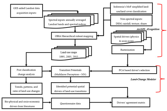
Figure 2.
Methodological approach for the study.
We adopted the land-use classification scheme from Indonesia’s Ministry of Forestry [49]. The 13 land-uses classes pertaining to the BRB landscape were simplified into 11 classes as specified in Table 1. The decision to adopt this approach was for several reasons: (1) BRB covers 15 administrative boundaries making it suitable for a study at a regional scale with medium resolution dataset, (2) The objective of the study was to examine the role of general land-use classes without specifying the stages of the vegetation. The primary and secondary vegetation classes do not exhibit distinct differences in hydrological responses and are relatively similar under the medium resolution images. Regrouping the 13 classes into 11 classes (merging two forest classes and two mangrove classes) allows a synoptic view of the landscape condition pertaining to forest and mangrove general conditions and their roles to water resources and watershed management as well as policy making at a regional level.

Table 1.
Land-use classification scheme (adapted from Indonesia Ministry of Forestry, 2021).
We then performed object-based image analysis (OBIA) to map land-use using eCognition™ software version 9.0 [71]. The OBIA and ruleset classifier were adopted based on several considerations: (1) it can better handle the issues of pixel-based mapping in that it can represent the complexity of shape, pattern, texture, context, and knowledge, which all are usually required to better define the land-use classes [72], (2) it reduces the salt-pepper effect due to spectral variations, (3) the use of ruleset and expert knowledge is useful in dealing with spectral limitations [73,74] and often results in a higher accuracy [75]. One drawback of the OBIA approach is the heavy computation and potential error propagation due poor segmentation [75,76]. There are no agreed rules in the segmentation and numerous studies applied shape and compactness scales on the basis of visual appearances of the segmented objects [77,78,79]. The segmentation parameters (shape and compactness) were reviewed in the current work by testing the values with 0.1 increments, finally choosing values of 0.2 and 0.7, respectively, that produced the visually most satisfactory delineation of objects while allowing OBIA to run relatively quickly. Association of land-use distribution and ecological factors were examined to help determine the hierarchical ruleset to classify objects [80]. The ruleset approach incorporated spectral and non-spectral features of an object such as elevation, distance, texture homogeneity, shapes, lengths, and width of objects, which is useful for mapping objects with similar spectral features [81]. In the OBIA-ruleset, we considered frequently used spectral indices in land-use mapping such as normalized difference vegetation index (NDVI) and normalized difference built-up index (NDBI), as well as non-spectral indices such as grey level co-occurrence matrix (GLCM) homogeneity and texture [81,82,83]. The threshold values used to separate objects were obtained from trials on a series of samples of objects with known land-use classes based on ground surveys, aerial photos, and Google Street View images. This approach reduces the possibility of misclassification that can arise from random sampling [84]. The thresholds were calculated from average values and visual optimization for the land-use class differentiation. We acknowledge this approach introduces subjectivity to the ruleset; however, it is helpful in achieving computational efficiency by skipping complex non-linear optimization approaches.
In total, 52 aerial photographs were used to validate the 1995 map (823-point samples). For the 2005 and the 2015 maps, ground survey notes, Google Street View images and Google Earth (1776 points) were used. The maps were overlain with a 1 km × 1 km grid and the grid centroids were used as the sampling locations. Around each sampling location, a 30 m × 30 m square mimicking the Landsat resolution was generated, and observation was performed within this boundary. In cases where ground survey data validation data were not available in that rectangle, for example due to access constraints, but were available nearby in the same grid square, the sampling location was moved to the nearest point that provided ground survey data. Two validators were used. For assessing the accuracy of the maps, we used a contingency table [85]. A map with kappa accuracy above 80% was regarded as acceptable for use in land-use change modeling [31]. A pixel-based post-classification change detection was selected [86,87,88]. To minimize the presence of spurious change (1) radiometric correction and co-registration was applied before classification [89], (2) an OBIA approach was used to reduce the salt-pepper effect, contributing to avoidance of spurious changes [69], and (3) ancillary data and expert knowledge were used to check and, where necessary, modify the generated maps [83,84]. The spurious changes that could not be avoided were accepted as part of the associated errors of the maps.
2.3. Potential Land-Use Drivers from Spatial Modeling
The Terrset Land Change Modeler (LCM) was selected to model spatial drivers of land-use change. This platform has been widely applied in varying landscapes such as African grasslands [24] and Southeast Asian green space [31]. LCM quantifies the spatial drivers through change analysis, pattern analysis, calculation of change probability and performance reporting. Change analysis is conducted by overlaying two post-classification maps in LCM [13,90]. LCM is also equipped with a built-in module to examine spatial trends of changes. The pattern of change was modelled using a third order polynomial due to its suitability for mapping the changing patterns [91].
According to Eastman (2016) [91], the spatial pattern (also termed as trend of land-use change in LCM), was developed using a trend surface analysis (TSA) where polynomial equations for changes were calculated and interpolated. The generic equation fitted by LCM’s TREND module is
where Z is the distributed variable, in this case is the transition between two selected land-uses, α terms are the polynomial coefficients, and U and V are the locational coordinates. The TSA surfaces were then calculated by coding the pixels of a specific transition as 1 and pixels of no change as 0 and treating the values as if they were continuous values to which the surface Z is fitted [91,92]. The values of Z generated have no special significance but allow the degree and direction of transition trends to be mapped and can identify the hot spots of land-use changes [91,93]. Higher positive values of Z indicate areas with more transitions, lower negative values imply areas dominated by the opposite transition, while zero values indicate areas with no or few transitions [94,95,96,97].
In this study, our primary concerns are the biophysical and socio–economic drivers of land-use. Factors regarding land ownership and legal status might play roles in influencing the land-use dynamics. However, such data are unavailable in the BRB. We acknowledge this as one limitation in this modeling. In addition, recent observations show that there has been substantial agricultural occupation of national parks such as in Bromo Tengger Semeru national park and Taman Hutan Raya Suryo. This violation to the official land status implies the inability or inefficiency of land zoning plans in governing the land-use dynamics in the BRB. We generated 33 candidate spatial biophysical and economic drivers based on our best understanding of local and regional conditions, literature on Java and other relevant landscapes [7,32,98,99,100], suitability, data availability and accessibility for research use. The candidate spatial drivers were generated from varying rasterized datasets such as elevation, roads, rivers, zonation plans, and digital climatic variables. To avoid correlated inputs and help interpret results, principal component analysis (PCA) [97] was used. The PCA results in the loading factors of each variable or driver. The drivers selected were all variables having high loading factors (>0.55 or <−0.55) in the PC and number of PCs included was that >90% of the variance was explained (Table 2).
Table 2.
Twelve selected land-use change drivers from PCA analysis.
LCM has the ability to quantify the relationship between a set of spatial explanatory drivers and a particular land-use transition type. In this study, land-use transition types were not grouped into “sub-models”. LCM determined primary land-use change transitions by excluding those with extents less than 0.5% of the total area. Then, LCM used a multi-layer perceptron (MLP)—an extended artificial neural network, non-parametric approach to model the specified transition type [102]. The relative contribution of a driver to the R2 value defines its importance to the transition type. The overall importance of a driver was measured by summing its importance rank over all land-use transition types.
2.4. Potential Land-Use Drivers from Questionnaires
Questionnaires were distributed to two groups of land-users covering agricultural land-users (farmers) and urban land-users (housing residents) during fieldwork in December 2018–March 2019. The questionnaires were distributed in 10 of the 13 cities, each of which provided 20–40 land users/respondents (total N = 280). The questionnaire was close-ended in the form of multiple choices. The drivers covered in the questionnaires were based on relevant published literature [7,32,98,99,100] and are listed in Appendix A. Questionnaire forms explored the land-users’ points of view about land-use change; and represented local features as opposed to the broader-scale biophysical environment, and therefore cannot account for the interaction of variables over space [100]. The relative importance of a variable of driver group was measured as the proportion of responses identifying the particular variable as important. In this context, we used a qualitative approach to quantify the importance for the household-level responses. We considered the degree of dominance as a measure of a variable’s importance. Whenever the percentage of response for each variable exceeded or was equal to the threshold, we listed this as a perceived driver. The threshold was quantified as 100% divided by the number of variables within a driver group (set to 50% for a driver group with only 1 variable). On the other hand, the relative importance of a spatial driver (driver used in LCM), was assessed using the relative reduction of R2 when a variable was excluded. All variables showing no or negligible R2 reduction were considered relatively less important. To evaluate the agreement between LCM-selected drivers and land-user-perceived drivers, an agreement matrix adapted from [14,77] was used (Table 3).
Table 3.
Classes of agreement of a driver in geospatial and land-users approach.
3. Results
3.1. Land-Use Change Quantification
The land-use maps produced for 1995, 2005 and 2015 were considered good with overall accuracy higher than 80% when it was aggregated over the 11 land-use classes (81.7%, 76.9%, and 81.2%, respectively). The relatively low-class accuracy values for sand, and shrubs (average: 78.4, 77.8, see Appendix B) may be attributed to the large variability of plant types and compositions in shrubs and bushes. We combined dryland forest classes (2 and 3 in Table 1) and dryland agriculture classes (7 and 8 in Table 1) into only dryland forest and dryland agriculture. This led to increased overall kappa accuracies of 87.3%, 83.1%, and 83.0% for 1995, 2005, and 2015, respectively.
Figure 3 portrays the land-use in the BRB in 1995, 2005, and 2015 (detailed information is in Appendix C). Over the study period, in 1995 the BRB was clearly dominated by agricultural land-uses (dryland farming and rice-fields), accounting for 77% of the total area, which declined to 68% in 2015 (Figure 4A). A decline was also observed in most other land-use classes, with varying rates (Figure 4B). Dryland forest showed the largest decline rates followed by rice-fields. Built-up areas almost tripled in extent from 1995 to 2015 (7.1% to 19.9%). Shrub and bush coverage increased by 1.5% from 1995 to 2015. Forest loss was higher in the period 1995–2005 and slowed down in the period 2005–2015. As opposed to this, rice-field and dryland agricultural losses were higher in the period 2005–2015. Over these two decades, around 29% of the BRB landscape changed.
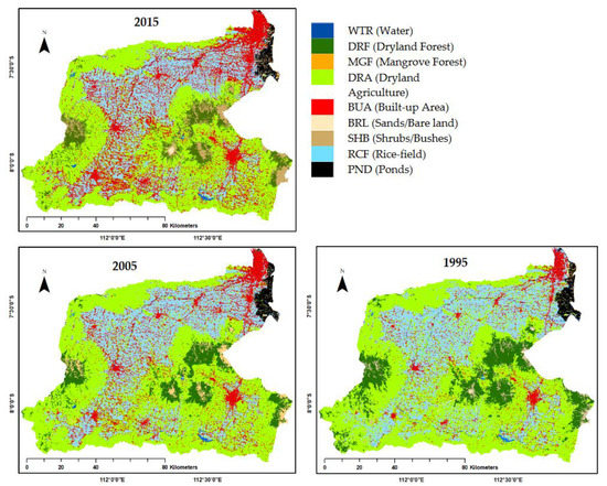
Figure 3.
Land-use maps of Brantas River Basin in 1995, 2005, and 2015.
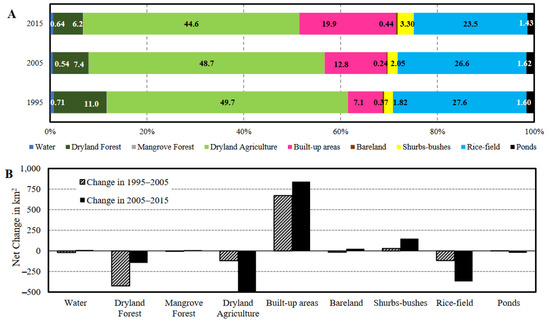
Figure 4.
Comparison of changes over land-use classes by: (A) percentage of study area, (B) gains and losses of area in km2.
The land-use changes in the BRB vary among cities (Figure 5). Urban expansion and agricultural decline occurred in all cities. The increases in built-up area ranged from 10% to 35%. A lower degree of urbanization (less than 15%) generally occurred in bigger cities than in smaller cities where agricultural land-uses are more evident. This might indicate bigger cities experience urban verticalization (leading to increasing population density without proportional increases in land-coverage).
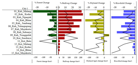
Figure 5.
City-wise changes in land-use during 1995–2015. The black line is the change relative to the city’s size (%), and the bars are the magnitude of changes (km2). The cities are ordered based on their size.
Post-classification change analysis allows us to examine types of transition as well as the extents. Figure 6 shows that over the two periods the ten largest land-use transitions were relatively consistent. In the period 1995–2005, 413 km2 of forest was converted to dryland agriculture. This extent dropped considerably in 2005–2015. Deforestation (including all land-use transitions from forest) and urbanization (all transitions to built-up areas) remain the largest transitions. Compared to rice-fields, dryland agriculture served as a bigger contributor to built-up areas. The most tangible transitions (>100 km2) are deforestation leading to shrubs and dryland agriculture, urbanization from rice-field and dryland farming loss, and the exchange from dryland farming to rice-fields and vice versa.
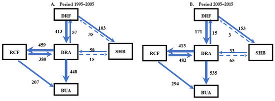
Figure 6.
Primary land-use transitions and their magnitude (in km2) for period (A) 1995–2005, (B) 2005–2015, DRF: dryland forest, DRA: dryland agriculture, SHB: shrubs/bushes, RCF: rice-fields, BUA: built-up areas.
3.2. Land-Use Transition Spatial Patterns (Trend of Changes)
Figure 7 provides the spatial patterns of four major land-use transitions generated from the LCM in the periods 1995–2005 and 2005–2015. Figure 7 shows that the patterns of land-use transition were visually similar between the two periods, suggesting that the drivers of land-use changes did not change much. It is evident from comparing Figure 1 with Figure 7A,B,E,F that the hotspots of forest conversion are associated with mountain regions. Considering the values from the TSA raster, the period 1995–2005 showed intense deforestation in the Arjuno-Kelud, Ngliman, and Bromo-Semeru mountain complexes. This was indicated by the concentration of high positive values of Z (Equation (1)) up to 0.130 (yellow to red). In 2005–2015, forest loss lessened as shown by the lowering positive values (maximum positive values 0.081) and was mostly found in Arjuno-Kelud. The transition from dryland to shrubs/bushes was also focused on mountain regions. Given the important role of dryland forests as tropical biodiversity hotspots, the results in Figure 5, Figure 6 and Figure 7 support the need for further investigations into changing biodiversity patterns in the region [78].
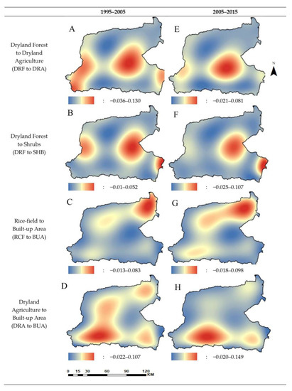
Figure 7.
Spatial patterns of deforestation and urbanization for 1995–2005 (A–D) and 2005–2015 (E–H).
Spatial trends in land-use transition suggest that urbanization did not occur uniformly across the BRB. It was evident that maximum positive values of Z in the second period increased from 0.083 to 0.098 for RCF to BUA and DRA to BUA, respectively. Spatially, the conversion of rice-fields to built-up areas was dominant in the northern part of the BRB, while dryland agricultural conversion was more intense in the middle and southern parts. While higher altitude areas exhibited forest loss, the lowland regions exhibited intense urbanization at the expense of rice-field and dryland farming. Urbanization of rice-field areas dominated in the northern lowlands, likely due to the industrialization of northern lowland cities, which has been evident over the last two decades due to government development policy. Urbanization of dryland farming areas was more evident in the middle to south-west BRB.
3.3. Potential Land-Use Drivers from Land Change Modeler
Table 4 lists LCM’s performance in modeling the major transitions, and the importance ranks of the tested drivers. Overall, the model performances were good (higher than 0.8) for afforestation and deforestation processes. Urbanization from rice-fields was modeled with lower accuracy (0.64) compared to urbanization from dryland (0.8). This infers that this process of urbanization is relatively complex. This transition (RCF to BUA) might also be introduced by the lower accuracy land-use maps for rice-field class (average land-use class accuracies: 80.50–83.70, Appendix B).
Table 4.
Relative importance of each driver for each land-use transition and model performance in explaining transitions.
We acknowledge that errors could propagate from the land-use mapping to the land-use driver analysis. The lower performances of the land-use transition model were generally related to transitions involving rice and shrub classes. This may be affected by the accuracy of land-use map inputs. Appendix B shows that the mapping of rice-fields and shrubs has relatively low accuracy (producer and user accuracies of 82.6% and 83.7%), while Table 4 shows that the four land-use transitions with the lowest R2 values (smaller than 0.75) are transitions that involve rice-field and shrubs. This implies that the accuracy of the land-use change modeling is controlling the accuracy of the transition model. Furthermore, there might be drivers affecting such transitions that cannot be spatially represented in the LCM platform. Socio–economic factors mostly operate at an individual scale and play a role in the family decision making process. Customs, family assets systems, living standards, capitals, poverty level, farming resilience, and personal perception, are types of factors influencing the decision-making process in land-use systems and often trigger the land-use change at individual level [14,103,104]. An example of how these factors work is exemplified by a household modeling of Deadman et al. [105] where a combination of physical land characteristics and household behavior such as subsistence requirements, number of capitals, and labors determine the decision in land utilization.
The results show that the importance of the driver depends on the transition type. Overall, elevation, distance to roads and city, and future economy zonation plans were relatively the most influential variables as identified from their higher influence (low scores). Drivers affecting forest loss were generally associated with elevation and proximity to roads and economic centers. Terrain constraints such as extreme slopes, thin soil, and low fertility might impede forest encroachment and make forests unsuitable for farming, leaving it to develop shrubs or secondary growth forest. Reports indicate that the main cause of deforestation in the BRB is illegal logging [106,107,108].
3.4. Perceived Land-Use Change Drivers
The questionnaire responses suggest the drivers that operate at land-user level (Table 5). In the housing sector, the four biggest portions of variables perceived by respondents were water facilities, water availability, growing population, and access/location with a portion of responses of 97%, 95%, 60%, and 39% of total respondents, respectively. About 2% of farmer respondents converted farming land into housing also for the needs of growing families. The growing population in the BRB during 2005–2015 [82] appears to be closely linked to the built-up area expansion. More than 90% of responses included facility networks and water availability suggesting that these factors influence conversion of land to housing. The prevalence of road access and location in responses also signifies the economic factors behind housing development.
Table 5.
Distribution of respondents’ responses on factors affecting land-use change.
Agriculture has long been a major livelihood for most people in the BRB. Farmers often change their plant types when facing less favorable conditions. Factors influencing farmers’ decisions to change plant types (also decisions to leave land fallow) included market-related factors, farming expenses, individual economic ability, technology/infrastructure, and biophysical conditions. Manpower availability was also seen to contribute to farmland persistence. The net gain and loss analysis in Figure 4B showed the decline in agricultural land-uses, and East Java statistical data showed the decreasing manpower in this sector [83]. Among these perceived drivers, market factors were the most essential (81%), followed by technology—machinery applications (54%), loans and subsidies (52%), and market guarantee (50%). Biophysical factors such as disaster hazards, and water availability were perceived only by 32% and 28% of farmers as factors contributing to change. Interestingly, policy and institutional factors were regarded as the least important, featuring in only 28% of responses.
3.5. Agreement between LCM-Based Drivers and Questionnaire-Based Drivers
Table 6 lists the driver groups and corresponding variables that were identified as important by both the questionnaire and LCM-based analysis. Natural hazards, rainfall variability, and accessibility in terms of locations, road network, and distance to farm were variables with a high degree of agreement. Biophysical variables were more dominant in the results of geospatial modeling, while anthropogenic variables such as economy, culture, technology, policy, and demography were only evident as land-user perceptions. These results allow inference about the degree of human–nature interaction. For example, from the geospatial approach, slope, elevation, and rainfall were statistically significant. Yet, only rainfall was perceived as an important driver. This implies that agricultural changes in BRB were more influenced by internal anthropogenic factors such as technology and market forces, and less by biophysical conditions. Due to the restriction of the questionnaire method to agricultural and urban land-users who were willing to participate, this method provides limited insight into drivers of encroachment into legally protected areas and changes from one public land use to another. For these questions, different approaches such as the use of participatory mapping, needs of informant connectors, indirect interviews, and focus group discussions would be required [84,85,86]. The results in Table 5 and Table 6 should be interpreted in context, predominant in the BRB, of legal transitions controlled by private landowners.
Table 6.
Agreement of inferred drivers from questionnaires and geo-statistical model.
4. Discussion
4.1. Land-Use Changes in the Brantas River Basin
Our results demonstrate how satellite image-based land use mapping was useful for presenting the 20-year dynamics of land-use changes in BRB. Post-classification change detection results from two land-use maps showed the snapshots of land-use changes in two periods, and thus identified the predominant land-use transitions in BRB. Massive urbanization has marked the changing landscape of the BRB from 1995 to 2015. Similar to other developing regions, the growing industrialization and economic zonation has led to urbanization [109] with, in this case, compensatory losses of rice-fields and dryland agriculture (Figure 6A,B). Post-classification change detection results show that urbanization appears to be the most stable process, meaning that once developed, there has been no or little chance to transform to other land-uses [90]. Dryland conversion to settlement occurred more intensely than rice-field conversion suggesting that rice-field conversion is less practicable. One plausible cause is that rice-fields in the BRB are mostly irrigated and the land price for irrigated areas is higher than for non-irrigated lands. In addition, current agricultural laws restrict conversion of irrigated lands (rice-fields) to other land-uses. This confirms the role of the socio–economic context in modifying the BRB landscape.
The spatial pattern of major land-use transitions in BRB highlights potential land use management problems. Both periods (1995–2005 and 2005–2015) were marked with forest conversion in mountain areas, massive rice conversion in the northern lowlands, and dryland farming loss mostly in the middle and southern lowlands. Considering that the forest concentration is at higher altitudes, the loss of forest would have hydrological consequences for lower regions with respect to intensified degradation. Increasing consequences in upper regions such as springs drying up, floods, and soil erosion have been increasingly reported [41]. Urban intensification in the lower BRB might exacerbate these consequences due to the increasing population exposed to floods, droughts, and poor-quality water supplies. Combating deforestation has been challenging and complex due to the socio–political context in Indonesia, such as enactment of local autonomy law [110].
4.2. Land-Use Transitions and Land-Use Patterns
At individual land-user level, the drivers are often related to external factors such as policy, socio–economic factors, and biophysical land conditions [27]. At this level, land-use change represents decision-making by land-users. Understanding these factors is essential in tropical developing regions as the transformation occurring in this level often leads to serious threats to sustainability. Therefore, besides quantitative modeling, a qualitative approach is commonly employed for investigating land-use change drivers [12,28].
Responses from local farmers in BRB inferred that agricultural land-use changes are not always related in simple ways to biophysical properties but also involve interactions of factors including cultural and socio–economic dimensions. For example, a study in upland Bromo (in south-eastern BRB) showed that improved roads led to better agricultural product delivery, which eventually triggered local people to cut down trees and convert to agriculture [111]. In this regard, roads appear to play a similar role in supporting continuing deforestation. It is important to note that agriculture remains a marginal sector for most farmers in BRB because most farmers have a small income (65% have an income < $USD 200). Respondents show a high dependence on the compilers not only for easy selling but also for loans, leaving fewer options for managing their lands. Compilers here refers to people buying farmers’ harvests on farm, often before harvest time at a lower than market price (this practice is termed “ijon”). Traditionally, compilers serve not only as buyers but also loan providers for farmers. In many cases, market prices can influence land-use conversions yet in the BRB this is not always the case. Around 25% of responses came from farmers stricken by minimum capital (low income, small land size, low education, lack of skills and experience) (Table 5), which to some degree explains why farmers may opt to keep growing the same crops. Efforts to convert land-use have implied that the processes are complex and involve several stages as outlined by [112]. Considering this, conversion of forest to new agricultural areas in the BRB might be associated with the easiest pathway to higher profits. The absence of alternatives to revenue generation has been acknowledged as a land degradation factor [113].
Information derived from the land-user questionnaires proved to be rich and detailed, qualitative, context-rich information able to be used to interpret land use management. These data were difficult to convert to objective measurements. With regards to the factors affecting the land users’ decisions, it is generally accepted that drivers at the individual level can vary and be unique [107,114,115]. This variability and uniqueness lead to challenges in designing questionnaires that comprehensively elucidate drivers—locally pertinent drivers may be missed.
4.3. Implication for Land-Use Change Modeling and Driver Assessment
LCM is a land-use model whose inputs are derived from varying geospatial datasets. For successful modeling, the accuracy of land-use map inputs is essential, and for this a high degree of land-use-map accuracy is preferable, with an 85% kappa accuracy sometimes used as a target [31]. Achieving high accuracy over areas with many land-use classes, such as the BRB, can be challenging. Generally, accuracy decreases with an increasing number of land-use classes [94]. This study utilized nine land-use classes with kappa accuracies of 87%, 83%, and 83% for the three studied years. Most previous LCM studies employed smaller numbers of land-use classes yet presented lower or similar LCM sub-model accuracies (39–91%) [24,116,117]. Despite the achievement of this study, there may be scope for better accuracy by optimizing the OBIA-mapping, which relied upon subjective selection of the ruleset.
Using both the questionnaires and geospatial modeling provided insight about the consistency and inconsistency between approaches in identifying drivers. Table 6, which only lists variables that were represented in both approaches, shows that biophysical variables were identified more commonly in the geospatial approach, while socio–economic and institutional variables were identified more commonly in the qualitative approach. One thing to note is that the PCA-based data reduction excluded some variables that were collinear with included variables from the geospatial analysis, so additional consistencies may be implicit. This might infer that variables which are significant at the regional level, might not be significant at the land-user level. Furthermore, as previously discussed, consistencies may be excluded due to the limitations of the geospatial data sets. We therefore acknowledge that the approach taken to understand the land-use change process is influenced by data and methodological limitations, in particular the challenge of integrating qualitative local-scale and geospatial regional-scale data sets requires further research. Decadal medium satellite image-based assessment cannot precisely outline the mechanism or process of each land-use trajectory, and further work is needed, that involves higher temporal resolution assessments and actual phenology characteristics.
4.4. Limitations of the Study
While the study has provided insight into the historic behavior of the landscape and drivers of changes, there are some limitations that are acknowledged and should be considered for future work. The first is that the study accommodated only the period 1995–2015 and excluded the more recent years, due to the lack of a complete decade. During these years, the BRB landscape is likely to have undergone and continue to undergo changes that may extend understanding of patterns and drivers of change and allow assessment of the medium-term impact of policies. Soon there will be opportunity to gain this further insight by updating the analysis to 2015–2025. There is also an opportunity to use our new understanding to project land-use change into the near future, 2025–2035, under policy scenarios, which we address in a separate work. From the geospatial modeling perspective, one limitation in this study’s approach is the decision to use regional-level land-use analysis. While this approach is proven to be computationally efficient, specific local land-uses such as airports and local sand mining could not be accounted for despite their known influence on the landscape. A future study with a more detailed land-use class scheme would offer opportunity to examine this issue.
The scale of the geospatial data also presents limitations. For example, in this study, district level population data (the only population data available for this study) does not represent demographic variability at a lower (village) level. Another challenge is whether, and how meaningfully, cultural variables can be represented as geospatial data layers. Factors such as social interaction and traditional customary land regulations cannot be easily represented in spatial data format. Land conflict, and the associated disagreements on zonation, lack of public access to data, and undocumented transitions from public to private land, create additional challenges in spatial data analysis. For example, there have been reports of land utilization for agriculture in national parks in Bromo Tengger Semeru (BTS) national park and Tahura Suryo (Suryo Grand Forest), which are supported by our visual assessment of high-resolution data from Google Earth. As a result, what was represented by legal spatial data (acknowledged park boundaries) might not always correspond with actual data (presence of farming gardens within park boundaries). The data availability limitations and complexity of specific factors affecting encroachment into protected areas are significant obstacles to a comprehensive understanding of land-use change drivers in the BRB and comparable regions and are perhaps the main limitation of this work. We recommend that, should the necessary data on land status become available, the research is extended to include this, and that complementary research attempts to understand the factors governing encroachment.
5. Conclusions
Over two decades (1995–2015), the BRB landscape has been marked by a reduction in vegetated areas. Forest area reduced from 1301 km2 to 730 km2 (11% to 6.2% of the total BRB area) and agricultural land-uses lessened from 9150 km2 to 8048 km2 (77% to 68%). A tripling in built-up areas signifies a rapidly urbanizing landscape. Major land-use transitions include forest conversion to dryland agriculture and agricultural area conversion to built-up area. The first phase of deforestation in the BRB is agricultural expansion, followed by conversion to built-up areas, which is nearly irreversible.
The biophysical and socio–economic drivers included in the geospatial modeling explain to a high degree the land-use transitions in the BRB over 1995–2015, which were mainly elevation, presence of roads, and access to urban centers and economic development centers. At land-user levels, the drivers are more complex and inter-related. The household and land-user questionnaires reveal (although incompletely) drivers that are localized and individualized. The questionnaire results were consistent with the geospatial modeling regarding the importance of rainfall, elevation, and access to economic centers, and thus provide high confidence about these results. The larger number of inconsistencies between the approaches set challenges for improved representation of cultural, demographic, and economic factors in geospatial modeling.
Author Contributions
Conceptualization, Bagus Setiabudi Wiwoho, Stuart Phinn, and Neil McIntyre; methodology, Bagus Setiabudi Wiwoho; software, Bagus Setiabudi Wiwoho; validation, Bagus Setiabudi Wiwoho; formal analysis, Bagus Setiabudi Wiwoho; writing—original draft preparation, Bagus Setiabudi Wiwoho; writing—review & editing, Stuart Phinn and Neil McIntyre; visualization, Bagus Setiabudi Wiwoho; supervision, Stuart Phinn and Neil McIntyre; funding acquisition, Bagus Setiabudi Wiwoho. All authors have read and agreed to the published version of the manuscript.
Funding
This research was funded by LPDP PhD scholarship grant BUDI-LN, contract number 201701220110184.
Data Availability Statement
Publicly available datasets were analyzed in this study. These data can be found from the URL provided in the methods section.
Acknowledgments
In this section, you can acknowledge any support given which is not covered by the author contribution or funding sections. This may include administrative and technical support, or donations in kind (e.g., materials used for experiments).
Conflicts of Interest
The authors declare no conflict of interest.
Appendix A
Table A1.
List of Drivers Implemented in Land-Users Questionnaire.
Table A1.
List of Drivers Implemented in Land-Users Questionnaire.
| Sector | Driver Group | Variables | Reference |
|---|---|---|---|
| Agriculture | Biophysical | Drought or flood or diseases | [118] |
| Infertile/unproductive/erosion | [26,119] | ||
| Natural water availability | [26,120] | ||
| Culture | Social empowerment | [15,121] | |
| Land contract/customary land tenure system | [17,32] | ||
| Demography/ population | Manpower availability | [26] | |
| Growing family members | [26] | ||
| Economy | Funding for farming practices | [15,32] | |
| Needs of urgent huge cash | [122] | ||
| Seeing peer/neighbor success (business) | [121] | ||
| High-cost land preparation and tillage | [15] | ||
| Market price fluctuation/low price | [23] | ||
| Access to buyers | [123] | ||
| Loans and subsidies availability | [15] | ||
| Infrastructure | Irrigation network | [7,124] | |
| Policy/ institutional | Network availability for direct selling—ease of selling | [32] | |
| Market guarantee | [125] | ||
| Awareness to planning policy and land administration responsibility | [15] | ||
| Technology | Agricultural technologies access and availability (i.e., seeds, fertilizers) | [17,126] | |
| Applying machineries | [126] | ||
| Housing | Biophysical | Natural beauty (site quality) | [124,127] |
| Natural water availability | [120,127] | ||
| Demography/ population | Basic need/growing family members | [128] | |
| Economy | Investment (business) | [129,130] | |
| Land/Housing Price | [15,128] | ||
| Infrastructure | Road access and location | [26] | |
| Distance to markets or school or workplace | [26] | ||
| Facilities (communication and electricity) | [15,127] | ||
| Policy/ institutional | Safety/crime | [127] | |
| Understanding to spatial plan zonation | [131] | ||
| Understanding to tax and land regulation | [130] |
Appendix B
Table A2.
Accuracy Assessment for Classified Images of BRB 1995, 2005, and 2015.
Table A2.
Accuracy Assessment for Classified Images of BRB 1995, 2005, and 2015.
| Land-Use | Code | 1995 | 2005 | 2015 | ||||||
|---|---|---|---|---|---|---|---|---|---|---|
| PA (%) | UA (%) | Average | PA (%) | UA (%) | Average | PA (%) | UA (%) | Average | ||
| Water | WTR | 92.31 | 85.71 | 89.01 | na* | na | na | 96.36 | 98.15 | 97.26 |
| Dryland forest | DRF | 100.00 | 100.00 | 100.00 | 100.00 | 100.00 | 100.00 | 100.00 | 86.11 | 93.06 |
| Mangrove forest | MGF | 86.59 | 94.04 | 90.32 | na | na | na | 89.36 | 95.89 | 92.63 |
| Dryland agriculture | DRA | 93.26 | 93.99 | 93.63 | 90.68 | 88.43 | 89.56 | 91.89 | 86.11 | 89.00 |
| Built-up areas | BUA | 86.84 | 91.67 | 89.26 | 89.13 | 93.18 | 91.16 | 81.89 | 87.83 | 84.86 |
| Sand/soil (bareland) | PST | 89.47 | 85.00 | 87.24 | 100.00 | 100.00 | 100.00 | 89.29 | 67.57 | 78.43 |
| Shrubs and bushes | SMB | 82.61 | 82.61 | 82.61 | 100.00 | 100.00 | 100.00 | 82.61 | 73.08 | 77.85 |
| Rice | SWH | 93.33 | 82.35 | 87.84 | 83.10 | 84.29 | 83.70 | 77.34 | 83.66 | 80.50 |
| Ponds | TBK | 96.15 | 96.15 | 96.15 | 100.00 | 100.00 | 100.00 | 92.68 | 97.44 | 95.06 |
| Overall accuracy (%) | 91.13 | 88.84 | 87.33 | |||||||
| Kappa accuracy (%) | 87.06 | 83.01 | 83.1 | |||||||
| Sample size | 823 | 251 | 1776 | |||||||
* No aerial photos used that have water and mangrove forest in the scene.
Appendix C
Table A3.
Land-Use Change Matrix of BRB for Period 1995–2004 and 2005–2015.
Table A3.
Land-Use Change Matrix of BRB for Period 1995–2004 and 2005–2015.
| LULC 1995 (km2) | LULC 2005 (km2) | ||||||||
|---|---|---|---|---|---|---|---|---|---|
| WTR | DRF | MGF | DRA | BUA | BRL | SHB | RCF | PND | |
| Water (WTR) | 49.38 | 0.02 | 0.49 | 11.76 | 5.46 | 0.65 | 0.00 | 12.35 | 3.79 |
| Dryland forest (DRF) | 0.26 | 781.95 | 0.00 | 413.20 | 0.78 | 0.44 | 103.38 | 1.85 | 0.00 |
| Mangrove forest (MGF) | 0.46 | 0.00 | 0.98 | 0.66 | 0.18 | 1.68 | 0.00 | 0.15 | 3.61 |
| Dryland agriculture (DRA) | 7.24 | 57.69 | 0.22 | 4889.48 | 448.67 | 5.51 | 14.48 | 459.63 | 3.44 |
| Built-up areas (BUA) | 0.00 | 0.00 | 0.00 | 0.00 | 841.64 | 0.00 | 0.00 | 0.00 | 0.00 |
| Bareland (BRL) | 1.02 | 1.05 | 0.42 | 10.17 | 5.18 | 9.42 | 5.16 | 4.35 | 6.44 |
| Shrubs and bushes (SHB) | 0.05 | 35.84 | 0.00 | 58.58 | 0.36 | 0.18 | 119.66 | 0.37 | 0.00 |
| Rice-field (RCF) | 3.48 | 0.27 | 0.00 | 380.85 | 207.77 | 2.55 | 0.17 | 2666.18 | 2.55 |
| Ponds (PND) | 2.12 | 0.02 | 0.94 | 1.69 | 3.13 | 7.40 | 0.00 | 1.69 | 171.82 |
| LULC 2005 (km2) | LULC 2015 (km2) | ||||||||
| WTR | DRF | MGF | DRA | BUA | BRL | SHB | RCF | PND | |
| Water (WTR) | 49.75 | 0.06 | 1.44 | 3.92 | 2.08 | 0.45 | 0.04 | 5.25 | 1.01 |
| Dryland forest (DRF) | 0.13 | 546.47 | 0.00 | 171.05 | 1.19 | 3.29 | 153.85 | 0.86 | 0.00 |
| Mangrove forest (MGF) | 0.17 | 0.00 | 2.11 | 0.00 | 0.00 | 0.42 | 0.00 | 0.02 | 0.32 |
| Dryland agriculture (DRA) | 12.57 | 151.53 | 1.18 | 4579.72 | 535.10 | 6.44 | 65.68 | 413.23 | 0.95 |
| Built-up areas (BUA) | 0.00 | 0.00 | 0.00 | 0.00 | 1513.16 | 0.00 | 0.00 | 0.00 | 0.00 |
| Bareland (BRL) | 0.27 | 0.22 | 2.41 | 3.03 | 4.10 | 8.43 | 0.63 | 2.77 | 5.97 |
| Shrubs and bushes (SHB) | 0.02 | 31.24 | 0.00 | 33.12 | 0.06 | 8.71 | 169.50 | 0.20 | 0.00 |
| Rice-field (RCF) | 11.73 | 1.17 | 0.15 | 482.29 | 294.31 | 5.60 | 0.27 | 2346.32 | 4.73 |
| Ponds (PND) | 1.13 | 0.00 | 5.55 | 0.37 | 3.70 | 18.70 | 0.00 | 6.17 | 156.05 |
References
- Faleiro, F.V.; Machado, R.B.; Loyola, R.D. Defining spatial conservation priorities in the face of land-use and climate change. Biol. Conserv. 2013, 158, 248–257. [Google Scholar] [CrossRef]
- Van Vliet, J.; de Groot, H.L.F.; Rietveld, P.; Verburg, P.H. Manifestations and underlying drivers of agricultural land use change in Europe. Landsc. Urban Plan. 2015, 133, 24–36. [Google Scholar] [CrossRef]
- Wagner, P.D.; Bhallamudi, S.M.; Narasimhan, B.; Kantakumar, L.N.; Sudheer, K.P.; Kumar, S.; Schneider, K.; Fiener, P. Dynamic integration of land use changes in a hydrologic assessment of a rapidly developing Indian catchment. Sci. Total Environ. 2016, 539, 153–164. [Google Scholar] [CrossRef] [PubMed]
- Xu, R.; Tian, F.; Yang, L.; Hu, H.; Lu, H.; Hou, A. Ground validation of GPM IMERG and TRMM 3B42V7 rainfall products over southern Tibetan Plateau based on a high-density rain gauge network. J. Geophys. Res. Atmos. 2017, 122, 910–924. [Google Scholar] [CrossRef]
- Rimal, B.; Baral, H.; Stork, N.E.; Paudyal, K.; Rijal, S. Growing city and rapid land use transition: Assessing multiple hazards and risks in the Pokhara Valley, Nepal. Land 2015, 4, 957–978. [Google Scholar] [CrossRef]
- Firman, T. Major issues in Indonesia’s urban land development. Land Use Policy 2004, 21, 347–355. [Google Scholar] [CrossRef]
- Partoyo; Shrestha, R.P. Monitoring farmland loss and projecting the future land use of an urbanized watershed in Yogyakarta, Indonesia. J. Land Use Sci. 2013, 8, 59–84. [Google Scholar]
- Margono, B.A.; Usman, A.B.; Sugardiman, R.A. Indonesia’s Forest Resource Monitoring. Indones. J. Geogr. 2016, 48, 7. [Google Scholar] [CrossRef]
- Bürgi, M.; Hersperger, A.M.; Schneeberger, N. Driving forces of landscape change-current and new directions. Landsc. Ecol. 2005, 19, 857–868. [Google Scholar] [CrossRef]
- Van Vliet, N.; Mertz, O.; Heinimann, A.; Langanke, T.; Pascual, U.; Schmook, B.; Adams, C.; Schmidt-Vogt, D.; Messerli, P.; Leisz, S. Trends, drivers and impacts of changes in swidden cultivation in tropical forest-agriculture frontiers: A global assessment. Glob. Environ. Chang. 2012, 22, 418–429. [Google Scholar] [CrossRef]
- Biazin, B.; Sterk, G. Drought vulnerability drives land-use and land cover changes in the Rift Valley dry lands of Ethiopia. Agric. Ecosyst. Environ. 2013, 164, 100–113. [Google Scholar] [CrossRef]
- Chebli, Y.; Chentouf, M.; Ozer, P.; Hornick, J.-L.; Cabaraux, J.-F. Forest and silvopastoral cover changes and its drivers in northern Morocco. Appl. Geogr. 2018, 101, 23–35. [Google Scholar] [CrossRef]
- Freitas, S.R.; Hawbaker, T.J.; Metzger, J.P. Effects of roads, topography, and land use on forest cover dynamics in the Brazilian Atlantic Forest. For. Ecol. Manag. 2010, 259, 410–417. [Google Scholar] [CrossRef]
- Kleemann, J.; Baysal, G.; Bulley, H.N.N.; Fürst, C. Assessing driving forces of land use and land cover change by a mixed-method approach in north-eastern Ghana, West Africa. J. Environ. Manag. 2017, 196, 411–442. [Google Scholar] [CrossRef]
- Lambin, E.F.; Geist, H.J. Regional differences in tropical deforestation. Environ. Sci. Policy Sustain. Dev. 2003, 45, 22–36. [Google Scholar] [CrossRef]
- Delphin, S.; Escobedo, F.J.; Abd-Elrahman, A.; Cropper, W.P. Urbanization as a land use change driver of forest ecosystem services. Land Use Policy 2016, 54, 188–199. [Google Scholar] [CrossRef]
- Verbist, B.; Putra, A.E.D.; Budidarsono, S. Factors driving land use change: Effects on watershed functions in a coffee agroforestry system in Lampung, Sumatra. Agric. Syst. 2005, 85, 254–270. [Google Scholar] [CrossRef]
- Bray, D.B.; Ellis, E.A.; Armijo-Canto, N.; Beck, C.T. The institutional drivers of sustainable landscapes: A case study of the ‘Mayan Zone’in Quintana Roo, Mexico. Land Use Policy 2004, 21, 333–346. [Google Scholar] [CrossRef]
- Kindu, M.; Schneider, T.; Teketay, D.; Knoke, T. Drivers of land use/land cover changes in Munessa-Shashemene landscape of the south-central highlands of Ethiopia. Environ. Monit. Assess. 2015, 187, 452. [Google Scholar] [CrossRef]
- Li, M.; Wu, J.; Deng, X. Identifying drivers of land use change in China: A spatial multinomial logit model analysis. Land Econ. 2013, 89, 632–654. [Google Scholar] [CrossRef]
- Rudel, T.K.; Defries, R.; Asner, G.P.; Laurance, W.F. Changing drivers of deforestation and new opportunities for conservation. Conserv. Biol. 2009, 23, 1396–1405. [Google Scholar] [CrossRef] [PubMed]
- Serneels, S.; Lambin, E.F. Proximate causes of land-use change in Narok District, Kenya: A spatial statistical model. Agric. Ecosyst. Environ. 2001, 85, 65–81. [Google Scholar] [CrossRef]
- Ostrom, E. A general framework for analyzing sustainability of social-ecological systems. Science 2009, 325, 419–422. [Google Scholar] [CrossRef] [PubMed]
- Gibson, L.; Münch, Z.; Palmer, A.; Mantel, S. Future land cover change scenarios in South African grasslands–implications of altered biophysical drivers on land management. Heliyon 2018, 4, e00693. [Google Scholar] [CrossRef]
- Verburg, P.H.; Soepboer, W.; Veldkamp, A.; Limpiada, R.; Espaldon, V.; Mastura, S.S.A. Modeling the spatial dynamics of regional land use: The CLUE-S model. Environ. Manag. 2002, 30, 391–405. [Google Scholar] [CrossRef]
- Verburg, P.H.; Bouma, J. Land use change under conditions of high population pressure: The case of Java. Glob. Environ. Chang. 1999, 9, 303–312. [Google Scholar] [CrossRef]
- Coral, C.; Bokelmann, W. The role of analytical frameworks for systemic research design, explained in the analysis of drivers and dynamics of historic land-use changes. Systems 2017, 5, 20. [Google Scholar] [CrossRef]
- Sorice, M.G.; Kreuter, U.P.; Wilcox, B.P.; Fox III, W.E. Changing landowners, changing ecosystem? Land-ownership motivations as drivers of land management practices. J. Environ. Manag. 2014, 133, 144–152. [Google Scholar] [CrossRef]
- Belay, T.; Mengistu, D.A. Land use and land cover dynamics and drivers in the Muga watershed, Upper Blue Nile basin, Ethiopia. Remote Sens. Appl. Soc. Environ. 2019, 15, 100249. [Google Scholar] [CrossRef]
- Fox, J.; Vogler, J.B. Land-use and land-cover change in montane mainland southeast Asia. Environ. Manag. 2005, 36, 394–403. [Google Scholar] [CrossRef]
- Nor, A.N.M.; Corstanje, R.; Harris, J.A.; Brewer, T. Impact of rapid urban expansion on green space structure. Ecol. Indic. 2017, 81, 274–284. [Google Scholar] [CrossRef]
- Suryanata, K. Fruit trees under contract: Tenure and land use change in upland Java, Indonesia. World Dev. 1994, 22, 1567–1578. [Google Scholar] [CrossRef]
- Erickson, D.L. Rural land use and land cover change: Implications for local planning in the River Raisin watershed. Land Use Policy 1995, 12, 223–236. [Google Scholar] [CrossRef]
- Mendoza, M.E.; Granados, E.L.; Geneletti, D.; Pérez-Salicrup, D.R.; Salinas, V. Analysing land cover and land use change processes at watershed level: A multitemporal study in the Lake Cuitzeo Watershed, Mexico (1975–2003). Appl. Geogr. 2011, 31, 237–250. [Google Scholar] [CrossRef]
- Tomer, M.D.; Schilling, K.E. A simple approach to distinguish land-use and climate-change effects on watershed hydrology. J. Hydrol. 2009, 376, 24–33. [Google Scholar] [CrossRef]
- Wang, R.; Kalin, L.; Kuang, W.; Tian, H. Individual and combined effects of land use/cover and climate change on Wolf Bay watershed streamflow in southern Alabama. Hydrol. Process. 2014, 28, 5530–5546. [Google Scholar] [CrossRef]
- Tu, J.; Xia, Z.-G.; Clarke, K.C.; Frei, A. Impact of urban sprawl on water quality in eastern Massachusetts, USA. Environ. Manag. 2007, 40, 183–200. [Google Scholar] [CrossRef]
- Wilson, C.O.; Weng, Q. Simulating the impacts of future land use and climate changes on surface water quality in the Des Plaines River watershed, Chicago Metropolitan Statistical Area, Illinois. Sci. Total Environ. 2011, 409, 4387–4405. [Google Scholar] [CrossRef]
- Surya, B.; Salim, A.; Hernita, H.; Suriani, S.; Menne, F.; Rasyidi, E.S. Land use change, urban agglomeration, and urban sprawl: A sustainable development perspective of Makassar City, Indonesia. Land 2021, 10, 556. [Google Scholar] [CrossRef]
- Margono, B.A.; Potapov, P.V.; Turubanova, S.; Stolle, F.; Hansen, M.C. Primary forest cover loss in Indonesia over 2000–2012. Nat. Clim. Chang. 2014, 4, 730–735. [Google Scholar] [CrossRef]
- Widianto, D.; Suprayogo, S.L.; Dewi, S. Implementasi Kaji Cepat Hidrologi (RHA) di Hulu DAS Brantas, Jawa Timur; World Agroforestry Centre ICRAF Southeast Asia Regional Office: Bogor, Indonesia, 2010. [Google Scholar]
- Nesheim, I.; Reidsma, P.; Bezlepkina, I.; Verburg, R.; Abdeladhim, M.A.; Bursztyn, M.; Chen, L.; Cisse, Y.; Feng, S.; Gicheru, P. Causal chains, policy trade offs and sustainability: Analysing land (mis) use in seven countries in the South. Land Use Policy 2014, 37, 60–70. [Google Scholar] [CrossRef]
- Hadiz, V. Reorganizing political power in Indonesia: A reconsideration of so-called’democratic transitions’. Pac. Rev. 2003, 16, 591–611. [Google Scholar] [CrossRef]
- Freedman, A.L. Economic crises and political change: Indonesia, South Korea, and Malaysia. Asian Aff. Am. Rev. 2005, 31, 232–249. [Google Scholar] [CrossRef]
- Aprianto, T.C. Perjuangan Landreform Masyarakat Perkebunan: Partisipasi Politik, Klaim, dan Konflik Agraria di Jember; STPN Press: Yogyakarta, Indonesia, 2016; ISBN 6027894296. [Google Scholar]
- Naylor, R.L.; Higgins, M.M.; Edwards, R.B.; Falcon, W.P. Decentralization and the environment: Assessing smallholder oil palm development in Indonesia. Ambio 2019, 48, 1195–1208. [Google Scholar] [CrossRef]
- Alaerts, G.J. Adaptive policy implementation: Process and impact of Indonesia’s national irrigation reform 1999–2018. World Dev. 2020, 129, 104880. [Google Scholar] [CrossRef]
- Timur, P.J. Rencana Tata Ruang Wilayah Propinsi Jawa Timur 2011–2031; Pemerintah Propinsi Jawa: Surabaya, Indonesia, 2011. Available online: https://bappeda.jatimprov.go.id/dokumen-perencanaan/ (accessed on 18 February 2023).
- Duncan, C.R. Mixed outcomes: The impact of regional autonomy and decentralization on indigenous ethnic minorities in Indonesia. Dev. Chang. 2007, 38, 711–733. [Google Scholar] [CrossRef]
- Firman, T. The continuity and change in mega-urbanization in Indonesia: A survey of Jakarta–Bandung Region (JBR) development. Habitat Int. 2009, 33, 327–339. [Google Scholar] [CrossRef]
- Tsujino, R.; Yumoto, T.; Kitamura, S.; Djamaluddin, I.; Darnaedi, D. History of forest loss and degradation in Indonesia. Land Use Policy 2016, 57, 335–347. [Google Scholar] [CrossRef]
- Winkler, K.; Fuchs, R.; Rounsevell, M.; Herold, M. Global land use changes are four times greater than previously estimated. Nat. Commun. 2021, 12, 2501. [Google Scholar] [CrossRef]
- Sang, X.; Guo, Q.; Wu, X.; Fu, Y.; Xie, T.; He, C.; Zang, J. Intensity and stationarity analysis of land use change based on CART algorithm. Sci. Rep. 2019, 9, 12279. [Google Scholar] [CrossRef]
- Chen, W.; Chi, G.; Li, J. The spatial association of ecosystem services with land use and land cover change at the county level in China, 1995–2015. Sci. Total Environ. 2019, 669, 459–470. [Google Scholar] [CrossRef] [PubMed]
- Austin, K.G.; Mosnier, A.; Pirker, J.; McCallum, I.; Fritz, S.; Kasibhatla, P.S. Shifting patterns of oil palm driven deforestation in Indonesia and implications for zero-deforestation commitments. Land Use Policy 2017, 69, 41–48. [Google Scholar] [CrossRef]
- Astuti, I.S.; Sahoo, K.; Milewski, A.; Mishra, D.R. Impact of land use land cover (LULC) change on surface runoff in an increasingly urbanized tropical watershed. Water Resour. Manag. 2019, 33, 4087–4103. [Google Scholar] [CrossRef]
- Neupane, M.; Dhakal, S. Climatic Variability and Land Use Change in Kamala Watershed, Sindhuli District, Nepal. Climate 2017, 5, 11. [Google Scholar] [CrossRef]
- Zhou, Y.; Li, X.; Liu, Y. Land use change and driving factors in rural China during the period 1995–2015. Land Use Policy 2020, 99, 105048. [Google Scholar] [CrossRef]
- Pawitan, H.; Haryani, G.S. Water resources, sustainability and societal livelihoods in Indonesia. Ecohydrol. Hydrobiol. 2011, 11, 231–243. [Google Scholar] [CrossRef]
- Pambudi, A.S.; Moersidik, S.S.; Karuniasa, M. Analysis of recent erosion hazard levels and conservation policy recommendations for Lesti Subwatershed, Upper Brantas Watershed. J. Perenc. Pembang. Indones. J. Dev. Plan. 2021, 5, 71–93. [Google Scholar] [CrossRef]
- Bhat, A. The politics of model maintenance: The Murray Darling and Brantas River Basins compared. Water Altern. 2008, 1, 201. [Google Scholar]
- Rijsdijk, A. Evaluating sediment sources and delivery in. Sediment Budg. 2005, 292, 16. [Google Scholar]
- Trianni, G.; Lisini, G.; Angiuli, E.; Moreno, E.A.; Dondi, P.; Gaggia, A.; Gamba, P. Scaling up to national/regional urban extent mapping using Landsat data. IEEE J. Sel. Top. Appl. Earth Obs. Remote Sens. 2015, 8, 3710–3719. [Google Scholar] [CrossRef]
- Goward, S.; Arvidson, T.; Williams, D.; Faundeen, J.; Irons, J.; Franks, S. Historical record of Landsat global coverage. Photogramm. Eng. Remote Sens. 2006, 72, 1155–1169. [Google Scholar] [CrossRef]
- Asgarian, A.; Soffianian, A.; Pourmanafi, S. Crop type mapping in a highly fragmented and heterogeneous agricultural landscape: A case of central Iran using multi-temporal Landsat 8 imagery. Comput. Electron. Agric. 2016, 127, 531–540. [Google Scholar] [CrossRef]
- Rocchini, D. Effects of spatial and spectral resolution in estimating ecosystem α-diversity by satellite imagery. Remote Sens. Environ. 2007, 111, 423–434. [Google Scholar] [CrossRef]
- Sidik, F.; Neil, D.; Lovelock, C.E. Effect of high sedimentation rates on surface sediment dynamics and mangrove growth in the Porong River, Indonesia. Mar. Pollut. Bull. 2016, 107, 355–363. [Google Scholar] [CrossRef]
- Vermote, E.; Justice, C.; Claverie, M.; Franch, B. Preliminary analysis of the performance of the Landsat 8/OLI land surface reflectance product. Remote Sens. Environ. 2016, 185, 46–56. [Google Scholar] [CrossRef]
- Leinenkugel, P.; Kuenzer, C.; Oppelt, N.; Dech, S. Characterisation of land surface phenology and land cover based on moderate resolution satellite data in cloud prone areas—A novel product for the Mekong Basin. Remote Sens. Environ. 2013, 136, 180–198. [Google Scholar] [CrossRef]
- Hadjimitsis, D.G.; Papadavid, G.; Agapiou, A.; Themistocleous, K.; Hadjimitsis, M.G.; Retalis, A.; Michaelides, S.; Chrysoulakis, N.; Toulios, L.; Clayton, C.R.I. Atmospheric correction for satellite remotely sensed data intended for agricultural applications: Impact on vegetation indices. Nat. Hazards Earth Syst. Sci. 2010, 10, 89–95. [Google Scholar] [CrossRef]
- Hegewisch, K. Climate Engine. Desert Research Institute and University of Idaho, 2017. Available online: https://www.lib.uidaho.edu/media/workshops/GISDay2017_Hegewisch.pdf (accessed on 18 February 2023).
- Deshpande, S.D.; Er, M.H.; Venkateswarlu, R.; Chan, P. Max-mean and max-median filters for detection of small targets. In Signal and Data Processing of Small Targets 1999; International Society for Optics and Photonics: Bellingham, DC, USA, 1999; Volume 3809, pp. 74–83. [Google Scholar]
- eCognition Developer, T. 9.0 User Guide; Trimble Germany GmbH: Munich, Germany, 2014.
- Blaschke, T.; Hay, G.J.; Kelly, M.; Lang, S.; Hofmann, P.; Addink, E.; Queiroz Feitosa, R.; van der Meer, F.; van der Werff, H.; van Coillie, F.; et al. Geographic Object-Based Image Analysis—Towards a new paradigm. ISPRS J. Photogramm. Remote Sens. 2014, 87, 180–191. [Google Scholar] [CrossRef]
- Hamedianfar, A.; Shafri, H.Z.M. Detailed intra-urban mapping through transferable OBIA rule sets using WorldView-2 very-high-resolution satellite images. Int. J. Remote Sens. 2015, 36, 3380–3396. [Google Scholar] [CrossRef]
- Li, X.; Myint, S.W.; Zhang, Y.; Galletti, C.; Zhang, X.; Turner, B.L., II. Object-based land-cover classification for metropolitan Phoenix, Arizona, using aerial photography. Int. J. Appl. Earth Obs. Geoinf. 2014, 33, 321–330. [Google Scholar] [CrossRef]
- Liu, D.; Xia, F. Assessing object-based classification: Advantages and limitations. Remote Sens. Lett. 2010, 1, 187–194. [Google Scholar] [CrossRef]
- Hussain, M.; Chen, D.; Cheng, A.; Wei, H.; Stanley, D. Change detection from remotely sensed images: From pixel-based to object-based approaches. ISPRS J. Photogramm. Remote Sens. 2013, 80, 91–106. [Google Scholar] [CrossRef]
- Guirado, E.; Blanco-Sacristán, J.; Rodríguez-Caballero, E.; Tabik, S.; Alcaraz-Segura, D.; Martínez-Valderrama, J.; Cabello, J. Mask R-CNN and OBIA fusion improves the segmentation of scattered vegetation in very high-resolution optical sensors. Sensors 2021, 21, 320. [Google Scholar] [CrossRef] [PubMed]
- Roelfsema, C.M.; Lyons, M.; Kovacs, E.M.; Maxwell, P.; Saunders, M.I. Multi-temporal mapping of seagrass cover, species and biomass: A semi-automated object based image analysis approach. Remote Sens. Environ. 2014, 150, 172–187. [Google Scholar] [CrossRef]
- Torres-Sánchez, J.; López-Granados, F.; Pena, J.M. An automatic object-based method for optimal thresholding in UAV images: Application for vegetation detection in herbaceous crops. Comput. Electron. Agric. 2015, 114, 43–52. [Google Scholar] [CrossRef]
- Blaschke, T. Object based image analysis for remote sensing. ISPRS J. Photogramm. Remote Sens. 2010, 65, 2–16. [Google Scholar] [CrossRef]
- Myint, S.W.; Gober, P.; Brazel, A.; Grossman-Clarke, S.; Weng, Q. Per-pixel vs. object-based classification of urban land cover extraction using high spatial resolution imagery. Remote Sens. Environ. 2011, 115, 1145–1161. [Google Scholar] [CrossRef]
- Chen, X.-L.; Zhao, H.-M.; Li, P.-X.; Yin, Z.-Y. Remote sensing image-based analysis of the relationship between urban heat island and land use/cover changes. Remote Sens. Environ. 2006, 104, 133–146. [Google Scholar] [CrossRef]
- Usman, M.; Liedl, R.; Shahid, M.A.; Abbas, A. Land use/land cover classification and its change detection using multi-temporal MODIS NDVI data. J. Geogr. Sci. 2015, 25, 1479–1506. [Google Scholar] [CrossRef]
- Palinkas, L.A.; Horwitz, S.M.; Green, C.A.; Wisdom, J.P.; Duan, N.; Hoagwood, K. Purposeful sampling for qualitative data collection and analysis in mixed method implementation research. Adm. Policy Ment. Health Ment. Health Serv. Res. 2015, 42, 533–544. [Google Scholar] [CrossRef]
- Story, M.; Congalton, R.G. Accuracy assessment: A user’s perspective. Photogramm. Eng. Remote Sens. 1986, 52, 397–399. [Google Scholar]
- Abd El-Kawy, O.R.; Rød, J.K.; Ismail, H.A.; Suliman, A.S. Land use and land cover change detection in the western Nile delta of Egypt using remote sensing data. Appl. Geogr. 2011, 31, 483–494. [Google Scholar] [CrossRef]
- Jensen, J.R.; Toll, D.L. Detecting residential land-use development at the urban fringe. Photogramm. Eng. Remote Sens. 1982, 48, 19820045797. [Google Scholar]
- Tewkesbury, A.P.; Comber, A.J.; Tate, N.J.; Lamb, A.; Fisher, P.F. A critical synthesis of remotely sensed optical image change detection techniques. Remote Sens. Environ. 2015, 160, 1–14. [Google Scholar] [CrossRef]
- Jianya, G.; Haigang, S.; Guorui, M.; Qiming, Z. A review of multi-temporal remote sensing data change detection algorithms. Int. Arch. Photogramm. Remote Sens. Spat. Inf. Sci. 2008, 37, 757–762. [Google Scholar]
- Xystrakis, F.; Psarras, T.; Koutsias, N. A process-based land use/land cover change assessment on a mountainous area of Greece during 1945–2009: Signs of socio-economic drivers. Sci. Total Environ. 2017, 587, 360–370. [Google Scholar] [CrossRef]
- Eastman, J.R. TerrSet Geospatial Monitoring and Modeling System–Manual; Clark University: Worcester, MA, USA, 2016. [Google Scholar]
- Chorley, R.J.; Haggett, P. Trend-surface mapping in geographical research. Trans. Inst. Br. Geogr. 1965, 47–67. [Google Scholar] [CrossRef]
- Václavík, T.; Rogan, J. Identifying trends in land use/land cover changes in the context of post-socialist transformation in central Europe: A case study of the greater Olomouc region, Czech Republic. GIScience Remote Sens. 2009, 46, 54–76. [Google Scholar] [CrossRef]
- Saifullah, K.; Barus, B.; Rustiadi, E. Spatial modelling of land use/cover change (LUCC) in South Tangerang City, Banten. In IOP Conference Series: Earth and Environmental Science; IOP Publishing: Bristol, UK, 2017; Volume 54, p. 12018. [Google Scholar]
- Islam, K.; Rahman, M.F.; Jashimuddin, M. Modeling land use change using cellular automata and artificial neural network: The case of Chunati Wildlife Sanctuary, Bangladesh. Ecol. Indic. 2018, 88, 439–453. [Google Scholar] [CrossRef]
- Gupta, R.; Sharma, L.K. Efficacy of Spatial Land Change Modeler as a forecasting indicator for anthropogenic change dynamics over five decades: A case study of Shoolpaneshwar Wildlife Sanctuary, Gujarat, India. Ecol. Indic. 2020, 112, 106171. [Google Scholar] [CrossRef]
- Vinayak, B.; Lee, H.S.; Gedem, S. Prediction of land use and land cover changes in Mumbai City, India, using remote sensing data and a multilayer perceptron neural network-based Markov chain model. Sustainability 2021, 13, 471. [Google Scholar] [CrossRef]
- Gray, D.A.; Chomitz, K.M.; Mundial, B. Roads, Lands, Markets, and Deforestation: A Spatial Model of Land Use in Belize; Banco Mundial: Washington, DC, USA, 1995. [Google Scholar]
- Handayani, W. Rural-urban transition in Central Java: Population and economic structural changes based on cluster analysis. Land 2013, 2, 419–436. [Google Scholar] [CrossRef]
- Overmars, K.P.; Verburg, P.H. Analysis of land use drivers at the watershed and household level: Linking two paradigms at the Philippine forest fringe. Int. J. Geogr. Inf. Sci. 2005, 19, 125–152. [Google Scholar] [CrossRef]
- Eastman, J.R.; Toledano, J. A short presentation of the Land Change Modeler (LCM). In Geomatic Approaches for Modeling Land Change Scenarios; Springer: Berlin/Heidelberg, Germany, 2018; pp. 499–505. [Google Scholar]
- Kamwi, J.M.; Cho, M.A.; Kaetsch, C.; Manda, S.O.; Graz, F.P.; Chirwa, P.W. Assessing the spatial drivers of land use and land cover change in the protected and communal areas of the Zambezi Region, Namibia. Land 2018, 7, 131. [Google Scholar] [CrossRef]
- Ewane, E.B. Land use land cover change and the resilience of social-ecological systems in a sub-region in South west Cameroon. Environ. Monit. Assess. 2021, 193, 338. [Google Scholar] [CrossRef]
- Deadman, P.; Robinson, D.; Moran, E.; Brondizio, E. Colonist household decisionmaking and land-use change in the Amazon Rainforest: An agent-based simulation. Environ. Plan. B Plan. Des. 2004, 31, 693–709. [Google Scholar] [CrossRef]
- Bank, W. Indonesia: Water Use Rights Study: Stage 2, Final Report Volume 1; 2004. Available online: https://documents.worldbank.org/en/publication/documents-reports/documentdetail/546631468263057128/annexes (accessed on 18 February 2023).
- Brun, C.; Cook, A.R.; Lee, J.S.H.; Wich, S.A.; Koh, L.P.; Carrasco, L.R. Analysis of deforestation and protected area effectiveness in Indonesia: A comparison of Bayesian spatial models. Glob. Environ. Chang. 2015, 31, 285–295. [Google Scholar] [CrossRef]
- Fulazzaky, M.A. Water quality evaluation system to assess the Brantas River water. Water Resour. Manag. 2009, 23, 3019–3033. [Google Scholar] [CrossRef]
- Wu, K.; Zhang, H. Land use dynamics, built-up land expansion patterns, and driving forces analysis of the fast-growing Hangzhou metropolitan area, eastern China (1978–2008). Appl. Geogr. 2012, 34, 137–145. [Google Scholar] [CrossRef]
- Purnomo, M.; Binternagel, N.; Faust, H. Transformation of resource management in Upland East-Java, Indonesia–From directive power to social and institutional interactions. In Proceedings of the Contributed Paper prepared for Presentation at the International Symposium ‘Sustainable Land Use and Rural Development in Mountainous Regions of Southeast Asia’, Hanoi, Vitnam, 21–23 July 2010; pp. 21–23. [Google Scholar]
- Lambin, E.F.; Geist, H.; Rindfuss, R.R. Introduction: Local processes with global impacts. In Land-Use and Land-Cover Change; Springer: Berlin/Heidelberg, Germany, 2006; pp. 1–8. [Google Scholar]
- Nawir, A.A.; Rumboko, L. History and state of deforestation and land degradation. For. Rehabil. Indones. Where After More Than Three Decad 2007, 11–32. [Google Scholar] [CrossRef]
- Goers, L.; Lawson, J.; Garen, E. Economic drivers of tropical deforestation for agriculture. Manag. For. Carbon A Chang. Clim. 2012, 305–320. [Google Scholar] [CrossRef]
- Gaveau, D.L.A.; Wandono, H.; Setiabudi, F. Three decades of deforestation in southwest Sumatra: Have protected areas halted forest loss and logging, and promoted re-growth? Biol. Conserv. 2007, 134, 495–504. [Google Scholar] [CrossRef]
- Ansari, A.; Golabi, M.H. Prediction of spatial land use changes based on LCM in a GIS environment for Desert Wetlands–A case study: Meighan Wetland, Iran. Int. Soil Water Conserv. Res. 2019, 7, 64–70. [Google Scholar] [CrossRef]
- Calijuri, M.L.; de Castro, J.S.; Costa, L.S.; Assemany, P.P.; Alves, J.E.M. Impact of land use/land cover changes on water quality and hydrological behavior of an agricultural subwatershed. Environ. Earth Sci. 2015, 74, 5373–5382. [Google Scholar] [CrossRef]
- Brown, D.G.; Walker, R.; Manson, S.; Seto, K. Modeling land use and land cover change. In Land Change Science; Springer: Berlin/Heidelberg, Germany, 2012; pp. 395–409. [Google Scholar]
- Jingan, S.; Jiupai, N.; Chaofu, W.; Deti, X. Land use change and its corresponding ecological responses: A review. J. Geogr. Sci. 2005, 15, 305–328. [Google Scholar] [CrossRef]
- Molden, D.; Oweis, T.Y.; Pasquale, S.; Kijne, J.W.; Hanjra, M.A.; Bindraban, P.S.; Bouman, B.A.M.; Mahoo, H.F.; Silva, P.; Upadhyaya, A. Pathways for increasing agricultural water productivity. In Water For Food Water For Life, A Comprehensive Assessment of Water Management; Earthscan: Oxford, UK, 2007. [Google Scholar]
- Martini, E.; Roshetko, J.M.; Paramita, E. Can farmer-to-farmer communication boost the dissemination of agroforestry innovations? A case study from Sulawesi, Indonesia. Agrofor. Syst. 2017, 91, 811–824. [Google Scholar] [CrossRef]
- Rondhi, M.; Pratiwi, P.A.; Handini, V.T.; Sunartomo, A.F.; Budiman, S.A. Agricultural land conversion, land economic value, and sustainable agriculture: A case study in East Java, Indonesia. Land 2018, 7, 148. [Google Scholar] [CrossRef]
- Umberger, W.J.; Reardon, T.; Stringer, R.; Mueller Loose, S. Market-channel choices of Indonesian potato farmers: A Best–Worst scaling experiment. Bull. Indones. Econ. Stud. 2015, 51, 461–477. [Google Scholar] [CrossRef]
- Campos, M.; Velázquez, A.; Verdinelli, G.B.; Skutsch, M.; Juncà, M.B.; Priego-Santander, Á.G. An interdisciplinary approach to depict landscape change drivers: A case study of the Ticuiz agrarian community in Michoacan, Mexico. Appl. Geogr. 2012, 32, 409–419. [Google Scholar] [CrossRef]
- Chomitz, K.M.; Gray, D.A. Roads, land use, and deforestation: A spatial model applied to Belize. World Bank Econ. Rev. 1996, 10, 487–512. [Google Scholar] [CrossRef]
- Geist, H.J.; Lambin, E.F. Proximate Causes and Underlying Driving Forces of Tropical DeforestationTropical forests are disappearing as the result of many pressures, both local and regional, acting in various combinations in different geographical locations. BioScience 2002, 52, 143–150. [Google Scholar] [CrossRef]
- Rahadi, R.A.; Wiryono, S.K.; Koesrindartoto, D.P.; Syamwil, I.B. Factors influencing the price of housing in Indonesia. Int. J. Hous. Mark. Anal. 2015. [Google Scholar] [CrossRef]
- Firman, T. Rural to urban land conversion in Indonesia during boom and bust periods. Land Use Policy 2000, 17, 13–20. [Google Scholar] [CrossRef]
- Adams Jr, R.H.; Cuecuecha, A. Remittances, household expenditure and investment in Guatemala. World Dev. 2010, 38, 1626–1641. [Google Scholar] [CrossRef]
- Monkkonen, P. Urban land-use regulations and housing markets in developing countries: Evidence from Indonesia on the importance of enforcement. Land Use Policy 2013, 34, 255–264. [Google Scholar] [CrossRef]
- Tutuko, P.; Shen, Z. The effect of land use zonings on housing development: The introduction of cdl approach in the border area of Surabaya and Sidoarjo Regency, Indonesia. Procedia-Soc. Behav. Sci. 2016, 227, 107–114. [Google Scholar] [CrossRef]
Disclaimer/Publisher’s Note: The statements, opinions and data contained in all publications are solely those of the individual author(s) and contributor(s) and not of MDPI and/or the editor(s). MDPI and/or the editor(s) disclaim responsibility for any injury to people or property resulting from any ideas, methods, instructions or products referred to in the content. |
© 2023 by the authors. Licensee MDPI, Basel, Switzerland. This article is an open access article distributed under the terms and conditions of the Creative Commons Attribution (CC BY) license (https://creativecommons.org/licenses/by/4.0/).