An Aggregated Shape Similarity Index: A Case Study of Comparing the Footprints of OpenStreetMap and INSPIRE Buildings

Abstract

The mutual identification of spatial objects is a fundamental issue when updating geographic data with other data sets. Representations of spatial objects in different sources may not have the same identifiers, which would unambiguously assign them to each other. Intersections of spatial objects can be used for this purpose, but this does not allow for the detection of possible changes and their quantification. The aim of this paper is to propose a simple, applicable procedure for calculating the shape similarity measure, which should be able to efficiently identify different representations of spatial objects in two data sources, even though they may be changed or generalised. The main result is the aggregated index of shape similarity and instructions for its calculation and implementation. The shape similarity index is based on the calculation of the set similarity, the distance of the boundaries, and the differences in the area, perimeter, and number of the vertices of areal spatial objects. In the case study, the footprints of the building complexes in Dúbravka (part of the city of Bratislava, the capital of Slovakia) are compared using data from OpenStreetMap and INSPIRE (Infrastructure for Spatial Information in Europe) Buildings. A contribution to the quality check of the OpenStreetMap data is then a secondary result. The proposed method can be effectively used in the semi-automatic integration of heterogeneous data sources, updating the data source with other spatial data, or in their quality control.

1. Introduction

Vector representations of spatial objects in two data sources are generally not identical. They can differ in position, size, shape, the number of vertices (nodes), but also the number of polygons in complex objects (Figure 1). When analysing spatial data from heterogeneous data sources or updating data from another one, it is important to determine whether it is a representation of the same spatial object or whether the object has been changed. The prerequisite for the integration or conflation [1,2] of such resources is the mutual identification of objects and the detection of possible changes that may have occurred over time. Attribute identifiers (primary keys) can be used to identify objects from each other, but only if they are the same in both sources. In practice, different representations of spatial objects mostly do not have the same identifiers. In this case, the intersections of areal spatial objects can be used. However, this method does not allow one to detect and quantify changes or differences between objects. For this purpose, we propose using a specially designed similarity measure. Our basic requirements also include the possibility of its simple calculation in an open-source geographic information system (GIS) or a spatial database management system.

Yan and Li [3] reviewed the definitions of similarity in various fields, including geometry, computer science, and geography. Let us emphasise that this paper is not about similarity in the sense of geometry but about the general meaning of the term similarity of shapes or spatial objects. Yan [4] defines the degree of spatial similarity as ‘a value between [0, 1], which is used to evaluate the similarity relations of spatial objects’. If both objects or their geometric representations are identical, their mutual similarity is 1 (identity), and if their sets of points do not have a non-empty intersection, the value of their mutual similarity is 0. We also use this principle to express the similarity of spatial objects.

In GIS and spatial analyses, several approaches were used to calculate similarity measures (see, e.g., [5,6,7,8,9,10]). Various correlation coefficients, set similarities, or distance measures are applied for this purpose [7,8,9,10,11,12]. They can be useful, for example, in data selection, cluster analysis, data harmonisation and integration, but also in data quality control [13,14,15]. Conflation, matching of spatial data and integration of heterogenous spatial data sources have already been discussed in several works [2,16,17,18,19,20,21]. Their goal was to combine the best quality objects from both data sources to create a composite dataset that is better than either of them [2] or automate data matching as much as possible [16,17,18,19]. According to [2], a geospatial conflation system requires efficient and robust geometrical and statistical algorithms, image processing and pattern recognition. In vector-to-vector conflation, focused mainly on road vector data, similarities of geometrical information can be used, such as nodes and lines [2,16,19,20]. Distance measures are generally used to determine the similarity of points or lines. According to [22], several researchers have applied the Euclidean distance method to evaluate the positional accuracy of point features, specifically in OpenStreetMap (OSM) [23,24,25]. Gil de la Vega et al. [26] analysed the most commonly used methods to evaluate the positional accuracy of linear features. They mentioned the average distance epsilon band, the Hausdorff distance, and the increasing buffer method [22,27]. However, the evaluation of the positional accuracy of areal objects is much more complex. For example, in the articles [28,29,30] the distance between the centroid of two polygons was used as a measure of similarity or its simple part. However, this parameter does not uniquely identify objects and does not sufficiently quantify their similarity. Even according to [28], it is difficult to define meaningful similarity measures for polygons with different numbers of vertices. Articles [31,32,33] also deal with the similarity and conflation of areal objects. According to [33], for polygon similarity measure is needed that compares polygons, not only point sets, with different numbers of vertices. For example, in [31], the total area of the overlapped building parts divided by the total area of the reference building was used.

In semi-automatic matching or conflating areal spatial objects, similarity measures can also be helpful [17,21]. They are based, for example, on the calculation of centroids and distances between them, buffers, the geographic context of objects [16,18], using a statistical approach [19], etc. Measuring the success of conflation using various measures is described, e.g., in [34]. The calculation of similarity measures should make it possible to effectively identify different representations of spatial objects, especially when integrating several heterogeneous data sources, updating one data source with another, or checking the quality of spatial data. However, automated or semi-automated conflation based on similarity measures is still an active research issue [1]. Therefore, this paper aims to propose and apply a generally applicable method for determining the degree of similarity of areal spatial objects, especially those representing buildings and their complexes. Its basic feature should also be the ease of application in GIS.

The proposed method is based on calculating the degree of similarity of the sets, the distance of the perimeter lines (boundaries) of two areal objects and differences in their parameters. In the case study, we apply it to compare two data sources, namely OSM [35] and INSPIRE (Infrastructure of Spatial Information in Europe), specifically for the quality assessment of building footprints. Quality control of OSM data is a very current topic due to its frequent use by a wide range of users in various applications [15,36,37,38,39,40]. The simple method of data evaluation could then also help to decide on their use for a specific purpose. We consider just buildings to be the most used areal objects from the OSM data. For example, works [41,42,43,44,45] are also devoted to the specific issue of quality control of OSM Buildings. A common problem in the evaluation of OSM data quality is the lack of a reference database from the same time [15]. In our study, we use available and up-to-date data, namely INSPIRE Buildings [46]. The area of the case study is Dúbravka, part of the city of Bratislava, the capital of the Slovak Republic.

The proposed method combines several concepts of similarity determination with the goal of expressing the similarity of areal objects as faithfully as possible, but also with the possibility of quick and simple implementation in GIS. In this paper, we, therefore, also present the implementation of the proposed procedure in QGIS 3.30 software [47] and the PostgreSQL 15 database management system [48] with the PostGIS extension [49].

Therefore, this work is structured as follows. Section 2 introduces the proposed method for calculating the shape similarity index and the data from the case study used. Section 3 reports on the similarity index calculation algorithm and the results of the case study. Section 4 and Section 5 include a discussion and conclusion.

2. Materials and Methods

2.1. Calculation of the Shape Similarity Index

To determine similarity or, in contrast, differences in representations of spatial objects, we propose the use of the aggregation of several measures of similarity or distance. The main idea is that the shape similarity index should consider the similarity of the object boundary but also its size, shape, and position. To determine the similarity of object boundaries, shapes, and positions, we propose using line distance measures (Section 2.1.2), which are sensitive to their changes. To determine the similarity of the size and position of objects, as well as the size of their mutual intersections, we propose to use similarity measures of sets (Section 2.1.3). This approach works with all points of area objects and considers them as a set. We also assume that the difference in area, perimeter, and number of vertices of two areal spatial objects can be useful to indicate the similarity of objects, especially in shape and size (Section 2.1.4). These parameters are easy to calculate and, moreover, show similarity even for objects that are similar but have a different position (moved or rotated objects). The general similarity index then aggregates all these measures (Section 2.1.5). Based on them, we also propose the procedure for deciding on the identity or change of objects. Therefore, our proposed method includes the calculation of multiple partial similarity measures of areal spatial objects, their aggregation, and the process of deciding on the identity or their changes.

An important requirement is also the possibility of determining similarity measures for special situations, such as moved and rotated areal objects (Figure 1c), generalised polygons (Figure 1a,d), or solving situations in which one areal object from the first source corresponds to several objects from the second source and vice versa (Figure 1b). Therefore, even before we apply the method of determining the degree of similarity of objects, it is necessary to identify pairs of areal objects that will be compared to each other, as this is not clearly established in various data sources. For this reason, especially in the case of buildings, we recommend comparing their complexes, not individual buildings (Section 2.1.1).

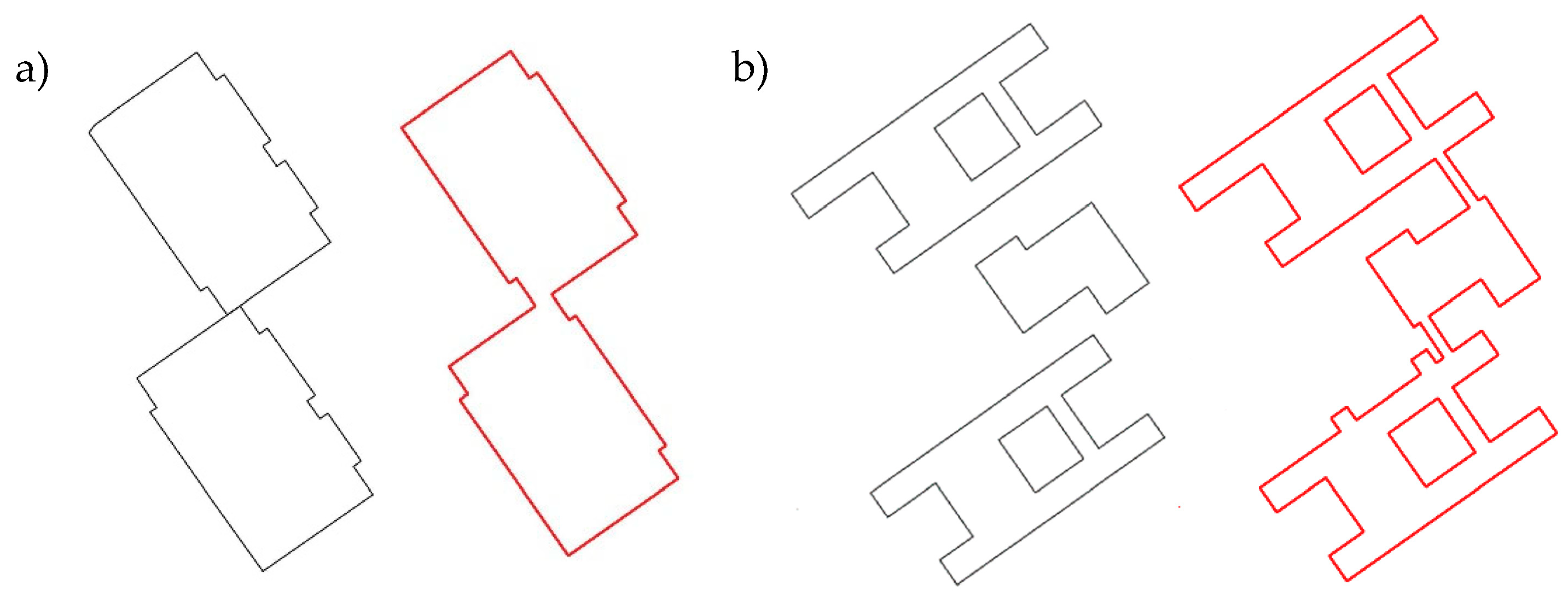
2.1.1. Matching Objects Identification

Before calculating the similarity measures, it is essential to identify the corresponding objects from both data sources. To do this, we first create their intersections. The calculation of similarity measures is feasible in this way if each object is represented by only one polygon (areal object). Figure 1a shows that one building in the first dataset corresponds to only one building from the other. This situation with multiple 1:1 relationships is an ideal case that can occur when matching objects. In other words, an intersection identifies only one pair of areal objects. However, there are common situations in which the relationships between objects are 1:N or M:N, or even 0:1 and 0:N in the case of objects missing from one of the databases. In the case of 1:N or M:N relationships, the intersections do not directly identify the corresponding objects (Figure 1b,d). Therefore, for our purposes, we recommend merging objects from the same data sources into larger units of mutually touching objects (buildings) and determining their similarity measures. Therefore, we compare building complexes rather than individual buildings. This way can also eliminate, or at least reduce, the number of ‘false intersections’ of mutually touching objects. Although this method does not allow one to determine the similarity of individual parts of the complex of buildings, it effectively solves the case where the building in the first data source is divided into several smaller parts in the second source. This case often occurs, for example, due to the different heights of some parts of the building stored as attributes (Figure 1b,d). This is also one of the common reasons for dividing one building into multiple areal objects in datasets.

In the proposed methodology, we determine the similarity and distance measures only for objects that intersect each other (having a non-empty intersection). Therefore, it is necessary first to check whether mutually identical objects are not significantly moved, for example, by a wrong transformation. However, objects that do not intersect with other objects are found mostly in only one of the two data sources (0:1 or 0:N relationships). To find them, we can select objects from the first source that intersect data from the second source and then reverse the selection. This method also allows us to check the completeness of objects in both data sources.

2.1.2. Calculation of Line Distances and Line Similarity Measures

To determine the similarity of the boundaries of the areal objects, we use the distances of the lines. Many distance measures in GIS are based on the distance between two points. Standard distance measures such as the Euclidean distance can also be used to determine the similarity of two linear objects, but only if they have the same number of vertices that correspond to each other. For linear objects that represent waterways, roads, or boundaries of areal objects, this condition is generally not met. A typical situation in which it is needed to approach another method is a comparison of two objects when the first one is generalised and the second one is more detailed (Figure 1a). For that reason, it is necessary to apply a different concept to determine the degree of similarity [10]. Therefore, in this study, we use the Hausdorff distance [50] or the Fréchet distance [51,52] to determine the similarity of two general lines.

Hausdorff distance $d_H(x,y)$ between two lines x a y is defined as follows [50],

$$d_H(x,y)=\max (\underset{X\in x}{\mathrm{s}\mathrm{u}\mathrm{p}}\underset{Y\in y}{\mathrm{i}\mathrm{n}\mathrm{f}} d(X,Y),\underset{Y\in y}{\mathrm{s}\mathrm{u}\mathrm{p}}\underset{X\in x}{\mathrm{i}\mathrm{n}\mathrm{f}} d(X,Y)),$$

(1)

where sup is supremum, inf is infimum, and d(X, Y) is the basic metric in the plane that determines the distance between two points X and Y (it can be, for example, the Euclidean distance).

Fréchet distance $d_F(x,y)$ is mathematically defined as the distance between two functions, $x:\left[x_1,x_2\right]\to {\mathbb{R}}^n$ and $y:\left[y_1,y_2\right]\to {\mathbb{R}}^n$, determined by the relation

$$d_F(x,y)=\underset{h}{\mathrm{i}\mathrm{n}\mathrm{f}}\underset{t}{\mathrm{s}\mathrm{u}\mathrm{p}}\left|x\left(t\right)-y\left[h\left(t\right)\right]\right|,$$

(2)

where $\underset{t}{\mathrm{s}\mathrm{u}\mathrm{p}}\left|x\left(t\right)-y\left[h\left(t\right)\right]\right|$ is the supremum of Euclidean distance $\left|x\left(t\right)-y\left[h\left(t\right)\right]\right|$ with respect to $t\in \left[x_1,x_2\right]$ [51,52].

It is necessary to transform the distances into the interval [0, 1] to calculate the degree of similarity of two lines from their mutual distance, given that a small distance means a large similarity and vice versa. According to [53,54], similarities and distances can be interconverted using the following equation:

$$similarity=\frac{1}{1+distance}.$$

(3)

The main disadvantage of this approach is that the resulting value depends on the units used (for example, m, cm), which is not suitable in our case. The other similarity measures are unitless, so to aggregate them, we need the similarity measures derived from distances to be unitless, too. Therefore, to transform distance measures into values from 0 to 1, we prefer to use the following transformation

$$sim\text{\_}d=1-\mathrm{m}\mathrm{i}\mathrm{n}\left(\frac{d}{d_{max}},1\right),$$

(4)

where d is the distance between the two lines, and d_max is the maximum distance that can be considered as a measure of the proximity of objects. We can determine the maximum distance based on the positional accuracy of the data, for example, three times the positional root mean square error (RMSE) of the less accurate dataset.

2.1.3. Calculation of Similarity Measures of Sets

In this approach to determining similarity measures, we consider areal objects as sets of points. The similarity of sets, as a basic similarity measure, can be simply described as follows: Two sets are similar if they are approximately the same (identical). Two sets, A and B, are identical if

$$A=A\cap B=B.$$

(5)

The interpretation of the indefinite term ‘similar’ is based on the concept that the set of objects outside the intersection $A\cap B$ is ‘small’ compared with the union $A\cup B$ [55,56].

Areal spatial objects can be considered as a set of points. The similarity of two sets A and B can then be defined in accordance with the concept of maximum mutual intersection and minimum union using the Jaccard similarity coefficient [57,58]

$$sim\text{\_}J(A,B)=\frac{\left|A\cap B\right|}{\left|A\cup B\right|},$$

(6)

where $\left|(A\cap B)\right|$ and $\left|(A\cup B)\right|$ express the cardinality of the sets of intersection and union of the sets A and B. The cardinality of the sets that represent areal objects can be expressed by their area in the GIS environment. In addition, for application in the GIS environment [47], it is advisable to use the transformation of the Jaccard similarity coefficient (6) into Tanimoto form [59],

$$sim\text{\_}T(A,B)=\frac{\left|A\cap B\right|}{\left|A\right|+\left|B\right|-\left|A\cap B\right|},$$

(7)

because for each pair of sets A and B:

$$\left|A\right|+\left|B\right|-\left|A\cap B\right|=\left|A\cup B\right|.$$

(8)

The main advantage is that it does not require the application of the Union function, but only the Intersection and the Area, which are easier to apply in the calculation of similarity measures in GIS.

An alternative method to calculate the degree of similarity based on a similar principle is the use of the Dice similarity index [60], sometimes referred to as the Sørensen–Dice coefficient or index [61,62]

$$sim\text{\_}SD(A,B)=\frac{2\left|A\cap B\right|}{\left|A\cup B\right|+\left|A\cap B\right|}=\frac{2\left|A\cap B\right|}{\left|A\right|+\left|B\right|}.$$

(9)

Note that sim_T ≤ sim_SD, which can be used to aggregate them (Section 2.1.5).

Both similarity coefficients take values from the interval [0, 1]. The larger the index value, the more similar the objects are in terms of their point sets.

2.1.4. Calculation of Area, Perimeter, and Number of Vertices as Basic Characteristics to Determine the Shape Similarity of Areal Objects

When comparing two geometric shapes, it is useful to use differences in their areas, perimeters, and number of vertices as their basic quantitative characteristics. Therefore, even within the framework of the proposal of the new methodology, we also apply these easily calculated measures. In this case, the important issue is to create measures from the differences in areas, perimeters, and number of vertices, which will take on values from the scale of 0 to 1. A simple solution, based on a principle similar to determining the similarity of sets (Section 2.1.3), is as follows.

$$sim\text{\_}A=1-\frac{|{Area}_A-{Area}_B|}{\mathrm{m}\mathrm{a}\mathrm{x}({Area}_A,{Area}_B)},$$

(10)

$$sim\text{\_}P=1-\frac{|{Perimeter}_A-{Perimeter}_B|}{\mathrm{m}\mathrm{a}\mathrm{x}({Perimeter}_A,{Perimeter}_B)},$$

(11)

$$sim\text{\_}V=1-\frac{|{Vertices}_A-{Vertices}_B|}{\mathrm{m}\mathrm{a}\mathrm{x}({Vertices}_A,{Vertices}_B)},$$

(12)

where sim_A, sim_P, and sim_V are similarity measures of the area, perimeter, and vertices. Area_A, Area_B, Perimeter_A, Perimeter_B, Vertices_A, and Vertices_B are the areas, perimeters, and numbers of vertices of polygons A and B, respectively.

2.1.5. Aggregation of Similarity Criteria to Determine the General Similarity Index

To determine a comprehensive measure of similarity, which would include both the similarity of the boundary and the similarity of the area and position, we propose to create an aggregated shape similarity index (ASI), whose general form is as follows.

$$ASI=f(sim\text{\_}D,sim\text{\_}S,sim\text{\_}SH),$$

(13)

where sim_D (distance similarity), sim_S (set similarity), and sim_SH (shape similarity) are partial similarity measures.

For the aggregation of similarity criteria, we propose applying aggregation operators, also known as intersections or unions (triangular norms and conorms), from the theory of fuzzy sets [63]. These operators are appropriate to use when the values of the aggregated criteria take values from 0 to 1, which is also fulfilled in the case of similarity measures. Another convenient option is to use the average (AVG) function to aggregate the sub-indexes.

The choice of aggregation operator depends on the purpose for which the similarity measure is to be used. The basic method is the use of a standard t-norm (fuzzy AND, that is, the MIN function), which corresponds to the necessity of meeting all criteria. The resulting similarity measure will then be the value that corresponds to the smallest value of all the similarity criteria. However, in some cases, not all criteria must be met for objects to be considered similar (Figure 1a,c). If, for example, the fulfilment of one criterion is sufficient, we can use the standard union, i.e., the MAX function.

Therefore, in this study, we recommend aggregating the partial similarity measures sim_D, sim_S, and sim_SH as follows:

$$ASI=(sim\text{\_}D\cup sim\text{\_}S)\cap sim\text{\_}SH$$

(14)

and using specific indices (Section 2.1.2, Section 2.1.3 and Section 2.1.4.)

$$ASI=\left(\right(sim\text{\_}H\cup sim\text{\_}F)\cup (sim\text{\_}T\cap sim\text{\_}SD))\cap (sim\text{\_}A\cap sim\text{\_}P\cap \mathrm{s}\mathrm{i}\mathrm{m}\text{\_}\mathrm{V}),$$

(15)

where

sim_H—Hausdorff distance similarity index,

sim_F—Fréchet distance similarity index,

sim_T—Tanimoto (Jackard) similarity index,

sim_SD—Sørensen–Dice similarity index,

sim_A—area similarity index,

sim_P—perimeter similarity index,

sim_V—vertices similarity index.

Applying the standard operations of fuzzy set theory and the fact that sim_T ≤ sim_SD (Section 2.1.3), we obtain the ASI index in a form suitable for implementation in GIS or a database system,

$$ASI=\min \left(\max \left(sim\text{\_}H,sim\text{\_}F,sim\text{\_}T\right),\mathrm{m}\mathrm{i}\mathrm{n}\left(sim\text{\_}A,sim\text{\_}P,sim\text{\_}V\right)\right).$$

(16)

The proposed index considers all the similarity factors included in the partial measures of similarity (position, distance, shape), as well as their individual characteristics. Note that the MAX function represents the standard union in the theory of fuzzy sets, while the intersection is expressed by the MIN function. Because sim_T ≤ sim_SD, we can omit sim_D in Formula (16). In the case of sim_SH, we suggest using the intersection of sim_A, sim_P, and sim_V. This also ensures cases where only the same area, perimeter, or number of vertices is not enough to establish their shape similarity. By applying the MAX aggregation function to sim_D and sim_S and then to sim_H, sim_F, and sim_T, we eliminate the influence of a possible unequal order of points when calculating the Hausdorff or Fréchet distance. To ensure all requirements, we finally determine the degree of similarity as the intersection of the mentioned sub-indices (using the MIN function).

In automatic object detection, areal objects can have a mutually different number of vertices, even if they are identical. In those cases, it is better to omit sim_V in the aggregated similarity index, especially if we apply the MIN function. This index defines neither a necessary nor a sufficient assumption of similarity. However, it can be useful for assessing the generalisation of areal objects. In addition, we recommend using one more parameter to determine it, namely based on the number of polygons in the polygon complex

$$sim\text{\_}POL=\mathrm{m}\mathrm{i}\mathrm{n}({Polygons}_A/{Polygons}_B{,Polygons}_B/{Polygons}_A),$$

(17)

where ${Polygons}_A$ and ${Polygons}_B$ are numbers of polygons of complexes A and B, respectively.

Its application helps to identify building complexes that can be considered identical but have a different number of polygons in individual data sources or are more generalised in one of them. In addition, it can be included in an algorithm to decide whether objects are likely to be similar or not.

2.2. Case Study and Data Used

In the case study, we compared two original data sources, specifically building footprints from OpenStreetMap data (OSM) [35] and a part of the Basic database for the geographic information system in the Slovak Republic (ZBGIS) [64] in the form of INSPIRE Buildings [46]. We applied the determination of similarity measures to the mutual identification of building footprints in areal vector data (polygons). The data used in the case study are also available in Supplementary Materials S1 and S2.

2.2.1. OpenStreetMap Data—OSM Buildings

OSM is a free and open global geographic database updated and maintained by a community of volunteers [35]. It is the largest and richest crowd-sourced geospatial database and the most successful Volunteered Geographic Information (VGI) project to date [36]. The OSM data are provided under the Open Database Licence (ODbL) published by Open Data Commons (https://opendatacommons.org/licenses/odbl/ (accessed on 10 July 2023)). The disadvantages of VGI can be considered as uneven spatial coverage and lack of data quality assurance, although many studies have shown that OSM has comparable or even better quality than authoritative data [37]. Of course, it depends a lot on the specific data and location.

In OSM, a ‘building’ is defined as ‘a man-made structure with a roof that is more or less permanently in one place’ (https://wiki.openstreetmap.org/wiki/Key:building (accessed on 10 July 2023)). OSM Buildings include their footprints, codes, names, and types. All OSM data are provided in the WGS84 coordinate reference system, mainly due to the ease of use of Global Navigation Satellite System (GNSS) devices for data collection.

2.2.2. INSPIRE Data—INSPIRE Buildings

The Infrastructure for Spatial Information in Europe (INSPIRE) [65] is based on the infrastructures for spatial information established and operated by the Member States of the European Union (EU). The INSPIRE Directive (https://eur-lex.europa.eu/eli/dir/2007/2/oj (accessed on 21 September 2023)) [66] provides a legal, technological, and organisational framework for its creation in all member states of the EU. Among other things, it addresses 34 spatial data themes needed for environmental applications, with key components specified through technical implementing rules (https://inspire.ec.europa.eu/data-specifications/2892 (accessed on 21 September 2023)). The theme Buildings is part of Annex III of the INSPIRE Directive.

Data Specification on Buildings is described in [67]. According to the Data Specification, ‘Buildings’ are ’constructions above and/or underground that are intended or used to shelter humans, animals, things, the production of economic goods or the delivery of services and refer to any structure permanently constructed or erected on its site’. Terms such as ‘a part of a building’ or ‘a generalised building’ are also defined in this specification. The data specification does not require specific data quality to avoid excluding data from INSPIRE. However, it proposes consistency rules between the semantic level of detail and the geometric accuracy. The 2D surface representation of buildings is the most frequent in INSPIRE data, but the building can be captured by its footprint, roof edge, or envelope. INSPIRE data should be published in the ETRS89 coordinate reference system for areas on the Eurasian tectonic plate and in ITRS elsewhere. In Slovakia, the base for INSPIRE Buildings data is the ZBGIS database provided by the Geodesy, Cartography and Cadastre Authority of the Slovak Republic (GCCA SR) [64].

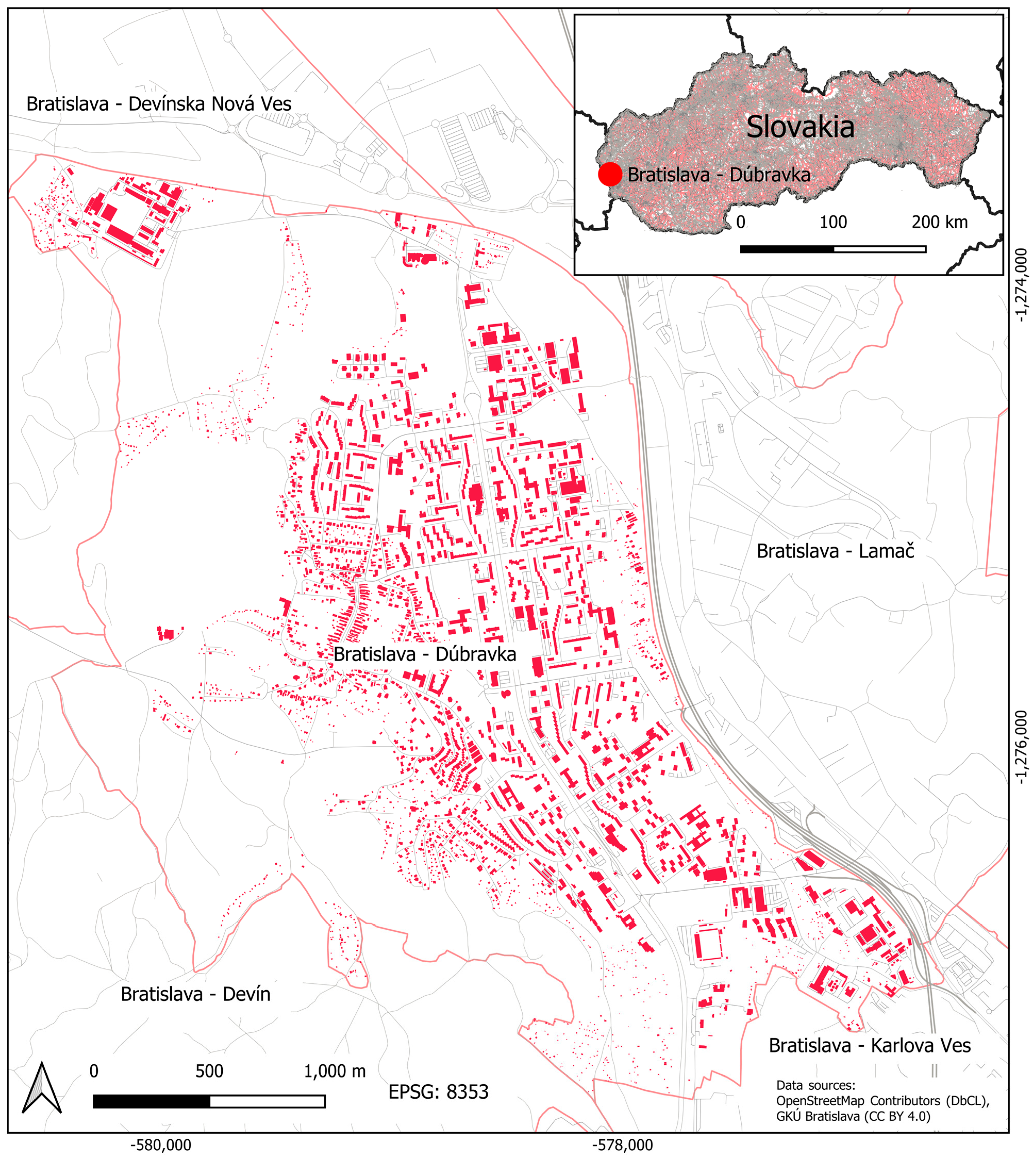
2.2.3. Area of Study

As a suitable area for the case study, we chose Dúbravka (Figure 2), part of Bratislava (the capital city of Slovakia), with an area of 8.6 km² and a population of approximately 39,000 (https://www.dubravka.sk/, accessed on 2 May 2023). The higher density of buildings in Dúbravka makes it more difficult to identify objects and is therefore suitable for a more complex case study. However, the main reason for its selection is that Dúbravka contains the old part with original unchanged buildings (the original village of Dúbravka), as well as many reconstructed or new buildings. In the old part of the Dúbravka district, there are the original buildings, such as an old church, chapel, historical buildings, original family houses, etc., but also reconstructed buildings (original houses after reconstruction or with extensions). In the new and peripheral parts of Dúbravka, there are also new objects which are not recorded in older data sources (e.g., new apartment and family buildings, multifunctional buildings, or a new shopping centre). Therefore, it contains many different types of buildings with a variety of footprints needed to demonstrate the proposed method (Figure 1, Figure 2, Figure 3 and Figure 6).

2.2.4. Comparison of OSM and INSPIRE Buildings Data Based on the Shape Similarity Index

In the case study, we used all 4186 INSPIRE Buildings and 3201 OSM Buildings that were in the databases in May 2023. There are more objects in INSPIRE Buildings than in OSM Buildings because they also contain the ‘building height’ attribute. This means that an object can be represented by several polygons (Figure 1b) whose height attribute is different in an attribute table (Section 2.1.1).

We used all buildings to compare both data sources. For the quality assessment of the OSM data, we used only those INSPIRE Buildings that are from the Database of Constructions (in which municipalities are obliged to register individual information required by law) [68] or data with high positional accuracy. Thus, we selected only 144 objects with a positional accuracy of 0.1 m. In addition, since the OSM Buildings are currently also updated with the data provided by GCCA SR, we used only objects obtained from two different sources. Of course, temporal accuracy is also limited by the date of the database update.

3. Results

The main result of this paper is the design of a new shape similarity index and algorithm for the identification of spatial objects or the determination of their similarity (Section 3.1 and Section 3.2). Another important result is a demonstration of the implementation of the solution in the QGIS and PostgreSQL environment with the PostGIS extension (Section 3.3).

The secondary result (Section 3.4) is the determination of the similarity measures in the case study, namely the comparison of the INSPIRE Building database and the OSM Buildings in Dúbravka (Bratislava, Slovak Republic).

3.1. Procedure for Calculation of the Shape Similarity Index

The brief procedure for calculating the similarity index in the GIS environment is shown below.

• Transformation of data sources tab_A and tab_B (spatial tables) into the same reference coordinate system (if they are not in a unified system).
• Merging of touching areal objects in sources tab_A and tab_B (can be implemented as 0 m buffers buf_A and buf_B).
• Count the polygons in polygon complexes buf_A and buf_B.
• Create intersections of buf_A and buf_B and calculate their basic parameters: area, perimeter, and number of vertices (this step leads to the creation of a table Similarity_A_B for calculating similarity indices).
• Calculation of auxiliary indices of similarity:
  • Dice and Tanimoto indices (sim_SD, sim_T),
  • Hausdorff and Fréchet distances (d_H, d_F) and their transformation to similarity indices (sim_H, sim_F),
  • Similarity of areas, perimeters, numbers of vertices and numbers of polygons of buf_A and buf_B (sim_A, sim_P, sim_V, and sim_Polygons),
  • Distance similarity, set similarity, and shape similarity (sim_D, sim_S, sim_SH).
• Calculate the aggregated similarity indices (sim_min, sim_max, sim_avg, and sim_agr).
• Assign a category of similarity or change type (sim_cat).
• Calculate the basic statistical characteristics of the results (number of objects in all categories, average values of aggregated similarity indices).

This procedure can be used as a basic guide for implementation in GIS or spatial database systems. In this paper, we also provide a concrete example of the implementation of the calculation of the proposed shape similarity index (Section 3.3).

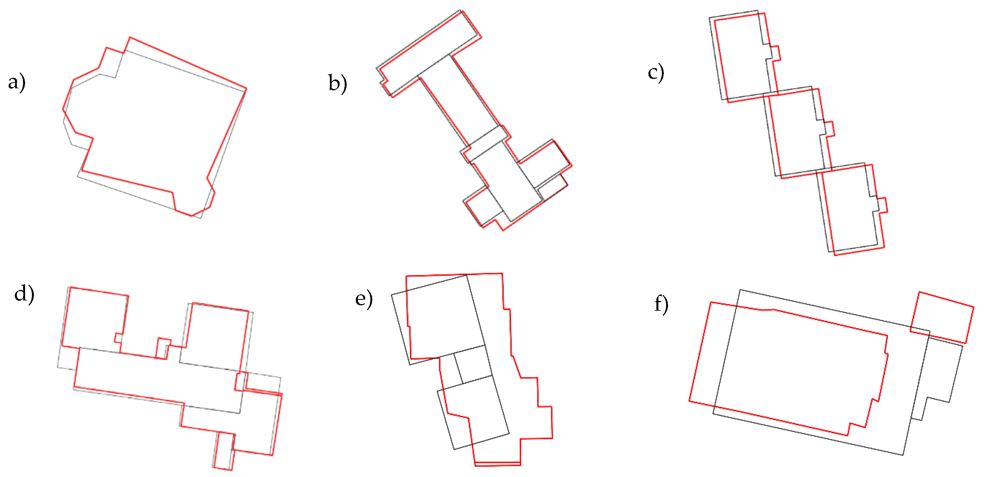
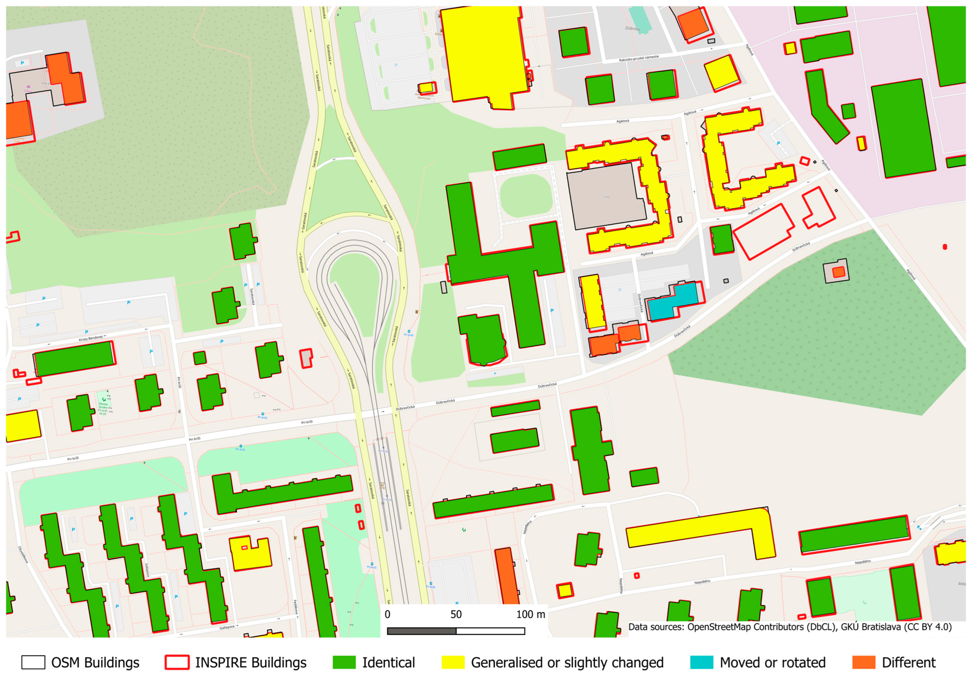
3.2. Classification of Objects According to Similarity Indices

When deciding on the identity or changes of building footprints, we propose to implement the classification rules shown in

Table 1. Selected sample cases of areal object similarity indices.

Distance Similarity	Set Similarity	Shape Similarity	Result	Example
~1 *	~1	~1	Similarity/Identity
~1	~1	~0	Changed or generalized object
~1	~0	~1	Impossible situations **	---
~1	~0	~0
~0	~1	~1
~0	~1	~0	A generalisation or, for example, an object contains a distant detail
~0	~0	~1	Moved or/and rotated object
~0	~0	~0	Changed object

~1 represents a high value, and ~0 represents a low value of the partial similarity index. ** impossible situations because if the distance similarity is ~1, then the set similarity and the shape similarity cannot be ~0 at the same time, and if the set similarity and the shape similarity are ~1, then the distance similarity must also be ~1.

and then use the following codes:

• 1—identical,
• 2—generalised or slightly changed,
• 3—moved or rotated,
• 4—different.

However, it is still necessary to establish criteria for inclusion into the above categories. For example, in our case, we use the following:

when ASI > 0.75,

   then ‘Identical’

when sim_min > 0.5 and (sim_d > 0.75 or sim_s > 0.75 or sim_area > 0.75),

   then ‘Generalised or slightly changed’

when sim_sh > 0.75 and sim_vertices > 0.75 and sim_s < 0.75,

   then ‘Moved or rotated’,

else ‘Different’.

We used the equal interval method for classification [69], so the interval boundaries for the four categories are 0, 0.25, 0.5, 0,75, and 1. The decision intervals would then be, for example: [0,0.25)—different; [0.25,0.5)—probably different; [0.5,0.75)—probably identical; and [0.75,1]—identical. However, we adapted them so that we could identify, for example, moved or generalised objects.

Note that the criteria can also be set individually according to a specific case study and a histogram of similarity index values.

3.3. Implementation of the Calculation of Aggregated Shape Similarity Indices

We implemented the calculation of the similarity indices and the classification of areal objects according to them in the PostgreSQL/PostGIS software environment. We used standard spatial functions such as ST_Transform, ST_Intersection, ST_Buffer, ST_Area, etc., but also special functions, for example, to calculate line distances. The use of the ST_FrechetDistance function in the PostgreSQL/PostGIS [70] requires the installation of GEOS (Geometry Engine—Open Source) of at least version 3.7.0. For the ST_HausdorffDistance function [71], the required version is at least 3.2.0. Although these are originally line similarity measures, they can be calculated both from the areal objects and their boundary lines.

We used special functions from the PostGIS extension to calculate distance measures. The advantage of applying the original Fréchet distance compared to the Hausdorff distance is that it considers the position and order of the points of the line. Unfortunately, only discrete Fréchet and Hausdorff distances, according to [72], are implemented in the PostGIS extension [70,71]. To refine the determination of the distance measure, we can use the densifyFrac parameter [71], but even this may not ensure an unambiguously correct determination of the distance measure. In other words, distance measures implemented in this way work well for similar objects (close to each other) but can be inaccurate for areal objects that have changed or are more distant from each other. Therefore, we suggest calculating both when determining line similarity in GIS. This is also the reason that it is not enough to apply only the distance measure to determine the similarity of line or polygon objects in GIS.

We also used the ST_NPoints function [73] to calculate the number of points in the geometry. The ST_Transform function is used to transform data into the same reference coordinate system. Specifically, in our case study, we used the EPSG:8353 coordinate system (S-JTSK [JTSK03] / Krovak East North) (https://epsg.io/8353, accessed on 2 May 2023). The SQL script is published in Supplementary Materials S3. The processing time for the case study was 12.67 s. The calculations were performed on a Windows computer with an Intel i7 processor with 16 GB of RAM.

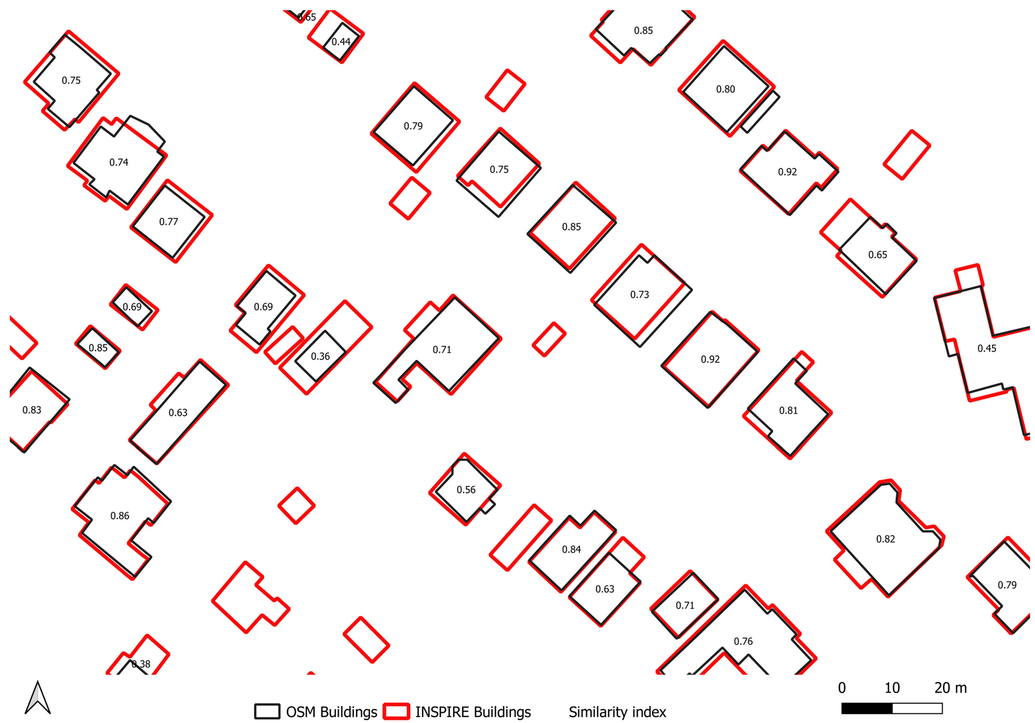
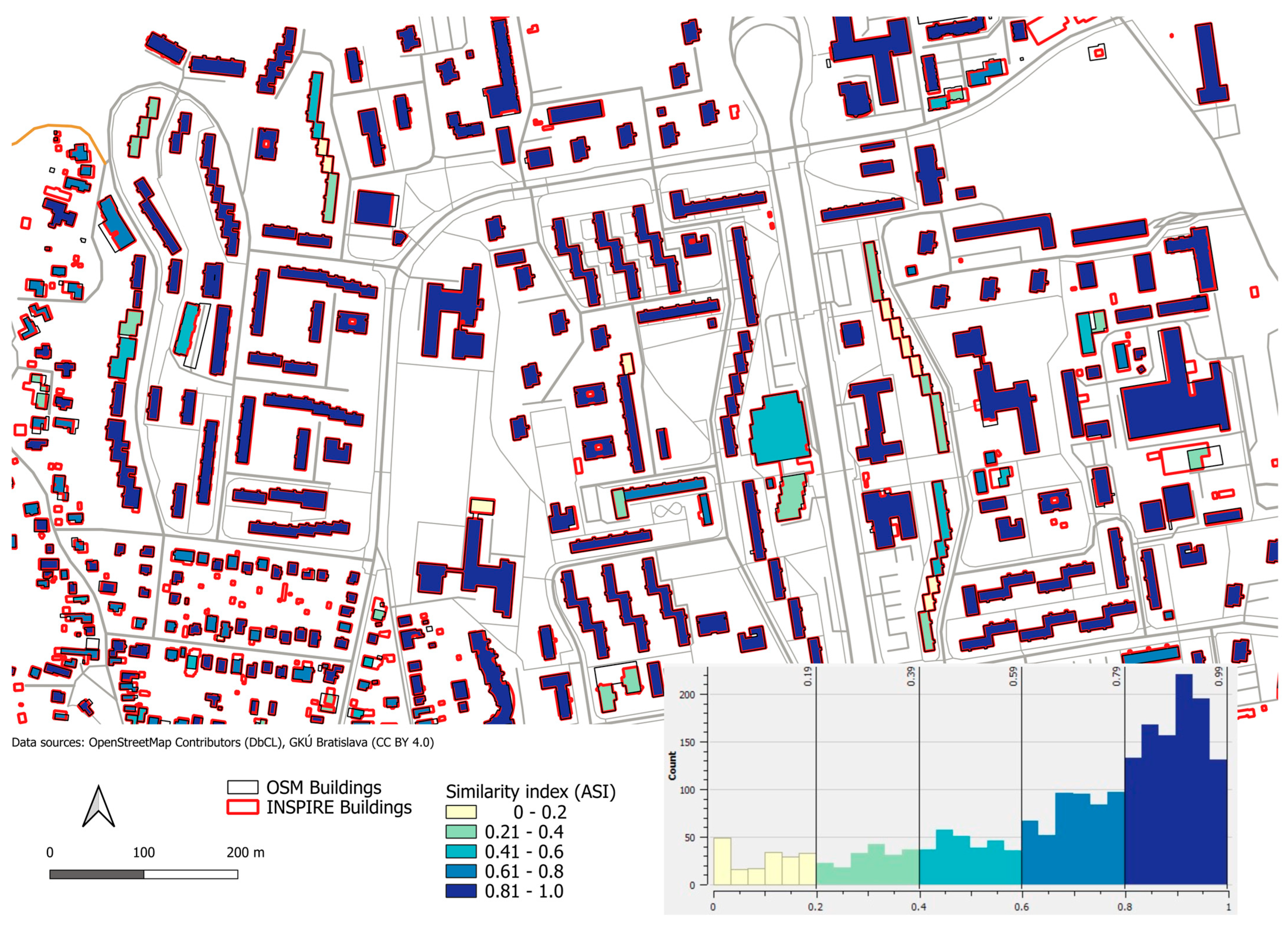
3.4. Comparison of OpenStreetMap and INSPIRE Building Complexes in Dúbravka Using Calculation and Visualisation of Similarity Indices of Building Footprints

As part of the case study, we analysed the similarity indices of all objects (building complexes) in Dúbravka. The total number is 2963 and 2201 for the INSPIRE and OSM buildings complexes footprints, respectively. A sample of the calculated aggregated shape similarity indices and their graphical representation in the QGIS environment is shown in Figure 3.

Table 2. A sample of values of selected partial similarity indices.

OSM (Black) and INSPIRE (Red) Buildings (Footprints)	Sim_H Sim_T Sim_A Sim_P Sim_V	OSM (Black) and INSPIRE (Red) Buildings (Footprints)	Sim_H Sim_T Sim_A Sim_P Sim_V
	0.44 0.64 0.21 0.57 1.00		0.59 0.82 0.49 0.71 0.71
	0.88 0.96 0.93 0.96 0.88		0.99 0.98 0.98 0.99 0.93

shows the partial similarity indices of several example objects in detail.

The general (average) shape similarity index of the INSPIRE and OSM Buildings in Dúbravka is 0.685. The frequency histogram of the aggregated shape similarity index and its classification into five equal intervals are shown in Figure 4.

Table 3. The number of objects in categories of object similarity classified in the case study in Dúbravka.

	Category of Object Similarity	Count
1.	Identical	1144
2.	Generalised or slightly changed	518
3.	Moved or rotated	10
4.	Different	453

shows the number of objects in each category of similarity in this case study. The visualisation of the classification into these categories is shown in Figure 5. According to Table 3, quite a lot of buildings are classified as ‘Different’. This can also be caused by buildings that are very close to each other but not connected (Figure 6a) or by multiple buildings being connected into one, for example, by a walkway (Figure 6b). These cases should be evaluated individually.

The proposed method can be used to detect changes in buildings or to find new or defunct buildings. In terms of assessing completeness or missing objects in both data sources (0:1 or 0:N relationships), we found the following. In the original data, there were 1145 INSPIRE Buildings that are not in the OSM and, conversely, 184 OSM Buildings that are not in the INSPIRE Buildings data. When analysing building complexes, 1037 of the INSPIRE data are not in the OSM, and 146 are missing in the INSPIRE data. We emphasise that these differences can be largely caused by the different semantics of the term ‘Building’ in individual data sources (Section 2.2.1 and Section 2.2.2).

3.5. OSM Buildings Data Quality Assessment

For an overall comparison of both data sources, we calculated the total index of similarity of all objects together (Section 3.4). However, data quality assessment requires field verification or at least the use of more accurate data. Therefore, we could only use 144 selected building footprints from the input data to evaluate the quality of the OSM Buildings. The positional accuracy of these objects in the INSPIRE Buildings data is 0.1 m. There were 123 of them in the OSM Buildings, which is 85%. Then, we selected 80 probably identical objects in both sources. The average aggregated shape similarity index of them is 0.82. This value also indicates the usability of the OSM data in terms of positional accuracy.

4. Discussion

4.1. Shape Similarity Index Calculation and Objects Classification

We recognise that there are multiple ways to design a shape similarity index. Several of them are also focused on the similarity of polygons or areal spatial objects [12,29,33,74,75]. In this study, we mainly focused on the basic properties of areal objects, as well as on the possibility of their simple implementation in open-source GIS software. We proposed an index of similarity of areal objects that considers their relative position, area, perimeter, similarity of sets representing polygons, and the distance of their boundaries. Thus, the proposed method combines some known concepts for determining the degree of similarity of areal objects but, at the same time, adds new approaches to them. The principle of determining various similarity measures when updating data with data from another source was also used in [58], where the calculation of the Jaccard and Dice similarity index was implemented in the ArcGIS software environment. In this paper, we extend the areal object identification procedure by calculating several other parameters, their aggregation, and implementation. In addition, the proposed index also considers the possibility that similar objects can be mutually displaced or rotated (Figure 1c, Table 1) or may have different degrees of generalisation of their boundaries (Figure 1a, Table 1), which is also an advantage compared to other methods of data conflation or integration.

The application of measures of distance, set similarities, and shape similarities ensures the calculation of the similarity index, which considers the position, size, and shape of the areal spatial objects. The distance calculation is also used to detect outliers on the boundaries of areal objects (Table 1). We are also aware that if, for example, the area, perimeter, and number of vertices are the same, the objects can still be different. Therefore, especially in the case of a difference or, in contrast, a match in the number of vertices, we eliminated this feature by choosing aggregation operators.

We also required the simplicity of the calculation and its feasibility in the environment of open-source GIS or spatial database systems. Although other methods can be more mathematically refined and also provide a good theoretical basis for data matching [6,16,17,18,19,20,21,75], the approach proposed by us is additionally easily implementable in current GIS environments using common tools. Therefore, its additional advantage is that it does not require the development and implementation of new functions and software tools. Because we process vector data stored in a spatial database, the method is also advantageous in terms of computational complexity (the calculation in the case study took only a few seconds).

The proposed methodology offers the possibility of simple and effective identification of spatial objects, updating spatial data with data from external sources, and managing their quality. This procedure can also be extended by determining the similarity of selected attributes (e.g., building type, height, or purpose of use). Then, the selection of an appropriate measure of attribute similarity is an important aspect of the entire process of determining the mutual similarity (or even likely identity) of objects.

A limitation of the method can be considered that it does not compare individual segments of buildings, for example, with different heights or other attributes, but rather their entire complexes. However, this can be an advantage in some cases (Section 2.1.1). The problem of how to deal with one-to-many or many-to-many relationships from the point of view of quality assessment is also indicated and solved, for example, in [13,14,15,29,76].

The similarity index is useful even without further classification and allows, for example, objects to be sorted by similarity. Even so, an open issue is also the choice of specific values of similarity measures when deciding whether objects are similar or changed. In this paper, we proposed classifying areal objects into four categories of similarity. An important choice is then the determination of the threshold values of the similarity indices at which the objects can be considered identical, changed, or different. According to [69], a definition of the class limits is the most difficult step in the classification process. Establishing a sharp boundary in the form of a specific value can be subjective. We partially solve this by applying multiple similarity coefficients, thereby reducing the possibility of making a wrong decision about the similarity of objects. However, without establishing decision criteria, it is not possible to use automated evaluation, decision-making about the identity or change of objects, or semi-automated data updating. In our case study, we used equal interval limits of 0.25, 0.5, and 0.75 to determine identical and changed areal objects, but other values or their interpretation could also be used [69]. The other commonly used methods to classify values in GIS [69,77,78] are quantiles, natural breaks classification [79], standard deviation classification, geometrical interval classification or manual classification in which breaks are placed at important user-defined threshold values. For example, to emphasise the strictness of a certain criterion, we can use a value of 0.95. In general, a similarity value of 0.75 (or 0.95) can indicate identity, 0.5 probable identity, and values < 0.5 correspond to the similarity of objects that require visual evaluation. However, it is much less than visual or manual inspection of all objects. Furthermore, for example, values < 0.25 may also directly indicate different or changed objects. The setting of values in the decision-making process can be changed depending on the accuracy and reliability of the input data. If it is necessary to include the uncertainty of the data in spatial analyses, we propose applying the principles of fuzzy set theory [10,80,81].

We implemented the proposed method in the widely used open-source software QGIS and PostgreSQL/PostGIS. Note that the algorithm is also suitable for use in other applications or platforms.

4.2. Case Study

Building data is a key theme for various spatial studies. OSM and INSPIRE data are among the most used sources of such data in Europe. The study [37] also analyses and compares the INSPIRE and OpenStreetMap data and considers them to be the most relevant initiatives for Europe in spatial data infrastructures (INSPIRE) and crowd-sourced geographic information projects (OSM). According to [37], combining INSPIRE and OSM data ultimately requires a comprehensive understanding not only of technical aspects but also of the processes underlying the creation and maintenance of the two infrastructures. Their up-to-dateness is also especially important. Therefore, in addition to determining similarity, it is necessary to detect missing and redundant objects in both input data sources or check the completeness of them.

However, the main goal of our work was not a real comparison of the two databases mentioned above. We realise that they arise under different conditions. The case study serves primarily as an example of the calculation of the spatial similarity index. Despite this, we can state relatively high values of similarity between these two data sources. The average value of the similarity index is 0.69, which is a very good result considering that it includes several different sub-indices, which it also strictly aggregates. This result is consistent with the results of previous works evaluating the quality of OSM data [14,37,44]. We also highlight the good similarity of the position despite the different originally referenced coordinate systems used. If the data were not correctly transformed, the similarity values could be much lower (for example, due to the displacement and rotation of objects). Based on the results of the case study, we also agree with the results of previous works [22,40,44,82,83] that it is important to verify the completeness of the OSM data. Even if the data were not complete in some areas, it can be used as an additional data source in integration with other data.

In the case of quality control, the resulting similarity index was even better, namely 0.82. It should be noted that the OSM data in Slovakia are currently also updated with data provided by the GCCA SR [64]. Of course, for the sake of correctness, we did not include such objects in quality control. That is also why there were only 123 objects in which we checked the data quality. The second reason was that we considered only objects with the highest positional accuracy (0.1 m) from the INSPIRE data source [46,68]. Although it is only a quality check on a small area and only on one layer of data, it can still be considered a contribution to the OSM data quality control, which is a very hot topic these days.

5. Conclusions

The purpose of this work was to propose and apply a suitable procedure to determine the similarity and probable identity of objects from various data sources in GIS for their integration or quality control. The novelty of the approach is mainly the aggregation of several appropriately designed subindices. They ensure control of the shape, size, position, and course of the border. We applied parameters such as Hausdorff distance, Fréchet distance, Tanimoto (Jackard) index, Sørensen–Dice similarity index, and differences in the area, perimeter, and number of polygon vertices. In addition, the proposed method includes classifying various areal objects into several categories of similarity or changes. It can deal with moved or rotated objects, polygons with holes, and multiple polygons in object complexes. Its implementation is easy because it is composed of freely available functions and tools in the GIS environment. As an example, we implemented it in open-source software, specifically QGIS and PostgreSQL with the PostGIS extension. The practical result of the work is also a sample of quality assessment of OSM data as one of the world’s most widely used sources of spatial data. We used INSPIRE Buildings as the second available data source. We compared building footprints as the most used areal objects in OSM. The testing was shown on a small sample of data, but the methodology is also applicable in larger studies containing data from different areas and multiple sources. The proposed method can then be used effectively in the semi-automated integration of multiple heterogeneous data sources, in updating a data source with other spatial data, or in spatial data quality control. In addition, the proposed methodology can also be applied to the same data source from two different periods for fast and effective change detection. We consider the possibility of reducing laborious manual data processing to be the main advantage of the mentioned procedure for identifying spatial objects and determining their similarity.

References

1. Lei, T.L. Geospatial Data Conflation. In The Geographic Information Science & Technology Body of Knowledge, 3rd Quarter 2019 ed.; Wilson, J.P., Ed.; UCGIS: Washington, DC, USA, 2019. [Google Scholar] [CrossRef]
2. Chen, C.C.; Knoblock, C. Conflation of Geospatial Data. In Encyclopedia of GIS; Shekhar, S., Xiong, H., Eds.; Springer: Boston, MA, USA, 2008; pp. 133–140. [Google Scholar] [CrossRef]
3. Yan, H.; Li, J. Spatial Similarity Relations in Multi-Scale Map Spaces; Springer International Publishing: Cham, Switzerland, 2015; 188p. [Google Scholar] [CrossRef]
4. Yan, H. Fundamental theories of spatial similarity relations in multi-scale map spaces. Chin. Geogr. Sci. 2010, 20, 18–22. [Google Scholar] [CrossRef]
5. Guo, N.; Shekhar, S.; Xiong, W.; Chen, L.; Jing, N. UTSM: A Trajectory Similarity Measure Considering Uncertainty Based on an Amended Ellipse Model. ISPRS Int. J. Geo-Inf. 2019, 8, 518. [Google Scholar] [CrossRef]
6. Jiang, X.; Huang, Y.; Zhang, F. Study on Spatial Geometric Similarity Based on Conformal Geometric Algebra. Int. J. Environ. Res. Public Health 2022, 19, 10807. [Google Scholar] [CrossRef]
7. Jiang, J.; Xu, J.; Lou, Y. Spatial Line Entity Matching Technology for Spatial Association of Multi-source Vector Data. In Proceedings of the 3rd International Conference on Big Data, Artificial Intelligence and Internet of Things Engineering (ICBAIE), Xi’an, China, 15–17 July 2022; pp. 523–527. [Google Scholar] [CrossRef]
8. Shahbaz, K. Applied Similarity Problems Using Frechet Distance. Ph.D. Thesis, Carleton University, Ottawa, ON, Canada, 2013. [Google Scholar]
9. Qiaoping, Z.; Deren, L.; Jianya, G. Shape similarity measures of linear entities. Geo-Spat. Inf. Sci. 2002, 5, 62–67. [Google Scholar] [CrossRef]
10. Xu, Y.; Xie, Z.; Chen, Z.; Xie, M. Measuring the similarity between multipolygons using convex hulls and position graphs. Int. J. Geogr. Inf. Sci. 2021, 35, 847–868. [Google Scholar] [CrossRef]
11. Ďuračiová, R.; Rášová, A.; Lieskovský, T. Fuzzy similarity and fuzzy inclusion measures in polyline matching: A case study of potential streams identification for archaeological modelling in GIS. Rep. Geod. Geoinform. 2017, 104, 115–130. [Google Scholar] [CrossRef]
12. Fan, H.; Zhao, Z.; Li, W. Towards Measuring Shape Similarity of Polygons Based on Multiscale Features and Grid Context Descriptors. ISPRS Int. J. Geo-Inf. 2021, 10, 279. [Google Scholar] [CrossRef]
13. Fan, H.; Zipf, A.; Jin, Y. Estimation of Building Types on OpenStreetMap Based on Urban Morphology Analysis. In Lecture Notes in Geoinformation and Cartography; Springer: Cham, Switzerland, 2014; pp. 19–35. [Google Scholar] [CrossRef]
14. Fan, H.; Zipf, A.; Jin, Y.; Neis, P. Quality assessment for building footprints data on OpenStreetMap. Int. J. Geogr. Inf. Sci. 2014, 28, 700–719. [Google Scholar] [CrossRef]
15. Başaraner, M. Geometric and semantic quality assessments of building features in OpenStreetMap for some areas of Istanbul. Pol. Cartogr. Rev. 2020, 52, 94–107. [Google Scholar] [CrossRef]
16. Saalfeld, A. Conflation Automated map compilation. Int. J. Geogr. Inf. Syst. 1988, 2, 217–228. [Google Scholar] [CrossRef]
17. Li, L.; Goodchild, M.F. Automatically and accurately matching objects in geospatial datasets. ISPRS Int. Arch. Photogramm. Remote Sens. Spat. Inf. Sci. 2010, 38, 98–103. [Google Scholar]
18. Kim, J.O.; Yu, K.; Heo, J.; Lee, W.H. A new method for matching objects in two different geospatial datasets based on the geographic context. Comput. Geosci. 2010, 36, 1115–1122. [Google Scholar] [CrossRef]
19. Walter, V.; Fritsch, D. Matching spatial data sets: A statistical approach. Int. J. Geogr. Inf. Sci. 1999, 13, 445–473. [Google Scholar] [CrossRef]
20. Ware, J.M.; Jones, C.B. Matching and aligning features in overlayed coverages. In Proceedings of the ACM SIGSPATIAL International Workshop on Advances in Geographic Information Systems, Washington, DC, USA, 6–7 November 1998. [Google Scholar]
21. Ledoux, H.; Ohori, K.A. Solving the horizontal conflation problem with a constrained Delaunay triangulation. J. Geogr. Syst. 2017, 19, 21–42. [Google Scholar] [CrossRef]
22. Moradi, M.; Roche, S.; Mostafavi, M.A. Exploring five indicators for the quality of OpenStreetMap road networks: A case study of Québec, Canada. Geoinformatica 2022, 75, 178–208. [Google Scholar] [CrossRef]
23. Girres, J.F.; Touya, G. Quality assessment of the French OpenStreetMap dataset. Trans. GIS 2010, 14, 435–459. [Google Scholar] [CrossRef]
24. Jackson, S.P. Analyzing Contribution Patterns of Volunteered Geographic Point Features in Relation to Errors and Demographics. Doctoral Dissertation, George Mason University, Fairfax, VA, USA, 2014. [Google Scholar]
25. Jonietz, D.; Zipf, A. Defining fitness-for-use for Crowdsourced points of interest (POI). ISPRS Int. J. Geo-Inf. 2016, 5, 149. [Google Scholar] [CrossRef]
26. Gil de la Vega, P.; Ariza-López, F.J.; Mozas-Calvache, A.T. Models for positional accuracy assessment of linear features: 2D and 3D cases. Surv. Rev. 2016, 48, 347–360. [Google Scholar] [CrossRef]
27. Goodchild, M.F.; Hunter, G.J. A simple positional accuracy measure for linear features. Int. J. Geogr. Inf. Sci. 1997, 11, 299–306. [Google Scholar] [CrossRef]
28. Cakmakov, D.; Arnautovski, V.; Davcev, D. A model for polygon similarity estimation. In Proceedings of the CompEuro 1992 Proceedings Computer Systems and Software Engineering, The Hague, The Netherlands, 4–8 May 1992; pp. 701–705. [Google Scholar] [CrossRef]
29. Kim, J.; Yu, K. Areal feature matching based on similarity using critic method. Int. Arch. Photogramm. Remote Sens. Spatial Inf. Sci. 2015, XL-2/W4, 75–78. [Google Scholar] [CrossRef]
30. Mahmoody-Vanolya, N.; Jelokhani-Niaraki, M.R. Measuring the spatial similarities in volunteered geographic information. ISPRS Ann. Photogramm. Remote Sens. Spatial Inf. Sci. 2023, X-4/W1-2022, 411–416. [Google Scholar] [CrossRef]
31. Song, W.; Haithcoat, T. Development of comprehensive accuracy assessment indexes for building footprint extraction. IEEE Trans. Geosci. Remote Sens. 2005, 43, 402–404. [Google Scholar] [CrossRef]
32. Latecki, L.J.; Lakämper, R. Shape similarity measure based on correspondence of visual parts. IEEE Trans. Pattern Anal. Mach. Intell. 2000, 22, 1185–1190. [Google Scholar] [CrossRef]
33. Avbelj, J.; Müller, R.; Bamler, R. A metric for polygon comparison and building extraction evaluation. IEEE Geosci. Remote Sens. Lett. 2015, 12, 170–174. [Google Scholar] [CrossRef]
34. Padilla-Ruiz, M.; López-Vázquez, C. Measuring conflation success. Rev. Cart. 2017, 94, 41–64. [Google Scholar] [CrossRef]
35. OpenStreetMap. Available online: https://www.openstreetmap.org (accessed on 10 July 2023).
36. Minghini, M.; Frassinelli, F. OpenStreetMap history for intrinsic quality assessment: Is OSM up-to-date? Open Geospat. Data Softw. Stand. 2019, 4, 9. [Google Scholar] [CrossRef]
37. Minghini, M.; Kotsev, A.; Lutz, M. Comparing INSPIRE and OpenStreetMap data: How to make the most out of the two worlds. Int. Arch. Photogramm. Remote Sens. Spatial Inf. Sci. 2019, XLII-4/W14, 167–174. [Google Scholar] [CrossRef]
38. Heris, M.P.; Foks, N.L.; Bagstad, K.J.; Troy, A.; Ancona, Z.H. A rasterized building footprint dataset for the United States. Sci. Data 2020, 7, 207. [Google Scholar] [CrossRef]
39. Basiri, A.; Jackson, M.; Amirian, P.; Pourabdollah, A.; Sester, M.; Winstanley, A.C.; Moore, T.; Zhang, L. Quality assessment of OpenStreetMap data using trajectory mining. Geo-Spat. Inf. Sci. 2016, 19, 56–68. [Google Scholar] [CrossRef]
40. Zhoua, Q.; Zhanga, Y.; Changa, K.; Brovellic, M.A. Assessing OSM building completeness for almost 13,000 cities Globally. Int. J. Digit. Earth 2022, 15, 2400–2421. [Google Scholar] [CrossRef]
41. Siebritz, L.-A. Assessing the Accuracy of OpenStreetMap Data in South Africa for the Purpose of Integrating it with Authoritative Data. Master’s Thesis, University of Cape Town, Cape Town, South Africa, 2014. [Google Scholar]
42. Müller, F.; Iosifescu, I.; Hurni, L. Assessment and visualization of OSM building footprint quality. In Proceedings of the 27th International Cartographic Conference, Rio de Janeiro, Brazil, 23–28 August 2015. [Google Scholar]
43. Zhang, H. Quality Assessment of the Canadian OpenStreetMap Road Networks. Master’s Thesis, University of Western Ontario, London, ON, Canada, 2017. [Google Scholar]
44. Borkowska, S.; Pokonieczny, K. Analysis of OpenStreetMap Data Quality for Selected Counties in Poland in Terms of Sustainable Development. Sustainability 2022, 14, 3728. [Google Scholar] [CrossRef]
45. OQ_Analysis. OpenStreetMap Quality Analysis Tools. Available online: https://github.com/pierzen/OQ_Analysis (accessed on 21 September 2023).
46. Geodesy, Cartography and Cadastre Authority of the Slovak Republic (GCCA SR). Geoportál. INSPIRE. Available online: https://www.geoportal.sk/en/inspire/download-data/ (accessed on 10 July 2023).
47. QGIS. Available online: http://qgis.com (accessed on 15 October 2023).
48. PostgreSQL. Available online: https://www.postgresql.org/ (accessed on 15 October 2023).
49. PostGIS. Available online: http://postgis.net (accessed on 21 September 2023).
50. Hausdorff, F. Grundzüge der Mengenlehre; Veit: Leipzig, Germany, 1914. [Google Scholar]
51. Alt, H.; Godau, M. Computing the Fréchet distance between two polygonal curves. Int. J. Comput. Geom. Appl. 1995, 5, 75–91. [Google Scholar] [CrossRef]
52. Ewing, G.M. Calculus of Variations with Applications; Dover Publications: New York, NY, USA, 1985. [Google Scholar]
53. Bajusz, D.; Rácz, A.; Héberger, K. Why is Tanimoto index an appropriate choice for fingerprint-based similarity calculations? J. Cheminform. 2015, 7, 20. [Google Scholar] [CrossRef]
54. Todeschini, R.; Ballabio, D.; Consonni, V.; Mauri, A.; Pavan, M. CAIMAN (classification and influence matrix analysis): A new approach to the classification based on leverage-scaled functions. Chemom. Intell. Lab. Syst. 2007, 87, 3–17. [Google Scholar] [CrossRef]
55. Bandemer, H. Mathematics of Uncertainty: Ideas, Methods, Application Problems; Springer: Berlin/Heidelberg, Germany, 2006; 190p. [Google Scholar]
56. Jaccard, P. Étude comparative de la distribution orale dans une portion des Alpes et des Jura. Bull. Soc. Vaudoise Sci. Nat. 1901, 37, 547–579. [Google Scholar]
57. Jaccard, P. Lois de distribution florale dans la zone alpine. Bull. Soc. Vaudoise Sci. Nat. 1902, XXXVIII, 68–130. [Google Scholar]
58. Ďuračiová, R.; Igondová, M. Integration of spatial data representing buildings by determining the degree of similarity. Czech J. Civ. Eng. 2017, 3, 29–35. [Google Scholar] [CrossRef]
59. Tanimoto, T. An Elementary Mathematical Theory of Classification and Prediction; Tech. Rep., IBM Report; IBM: New York, NY, USA, 1958. [Google Scholar]
60. Dice, L.R. Measures of the Amount of Ecologic Association Between Species. Ecology 1945, 26, 297–302. [Google Scholar] [CrossRef]
61. Sørensen, T. A method of establishing groups of equal amplitude in plant sociology based on similarity of species and its application to analyses of the vegetation on Danish commons. Biol. Skr. 1948, 5, 1–34. [Google Scholar]
62. Gragera, A.; Suppakitpaisarn, V. Relaxed triangle inequality ratio of the Sørensen–Dice and Tversky indexes. Theor. Comput. Sci. 2017, 718, 37–45. [Google Scholar] [CrossRef]
63. Grabisch, M.; Marichal, J.-L.; Mesiar, R.; Pap, E. Aggregation Functions, Encyclopedia of Mathematics and Its Applications; No 127; Cambridge University Press: Cambridge, UK, 2009. [Google Scholar]
64. Geodesy, Cartography and Cadastre Authority of the Slovak Republic (GCCA SR). ZBGIS. 2023. Available online: https://zbgis.skgeodesy.sk/mkzbgis/en/ (accessed on 15 October 2023).
65. INSPIRE. Available online: https://inspire.ec.europa.eu (accessed on 21 September 2023).
66. Commission of the European Communities. Directive 2007/2/EC of the European Parliament and of the Council of 14 March 2007 Establishing an Infrastructure for Spatial Information in the European Community (INSPIRE). 2007. Available online: https://eur-lex.europa.eu/eli/dir/2007/2/2019-06-26 (accessed on 21 September 2023).
67. European Commission. D2.8.III.2 INSPIRE Specification on Buildings—Technical Guidelines. 2013. Available online: https://inspire.ec.europa.eu/documents/Data_Specifications/INSPIRE_DataSpecification_BU_v3.0.pdf (accessed on 21 September 2023).
68. Geodesy, Cartography and Cadastre Authority of the Slovak Republic (GCCA SR). Zoznam Stavieb (List of Buildings). 2023. Available online: https://www.skgeodesy.sk/sk/ugkk/kataster-nehnutelnosti/zoznam-stavieb/ (accessed on 10 July 2023).
69. Kraak, M.; Ormeling, F. Cartography: Visualization of Geospatial Data, 4th ed.; CRC Press: Boca Raton, FL, USA, 2020; 261p. [Google Scholar]
70. ST_FrechetDistance. Available online: https://postgis.net/docs/ST_FrechetDistance.html (accessed on 21 September 2023).
71. ST_HausdorffDistance. Available online: https://postgis.net/docs/ST_HausdorffDistance.html (accessed on 21 September 2023).
72. Eiter, T.; Mannila, H. Computing Discrete Fréchet Distance. Technical University of Vienna. 1994. Available online: http://www.kr.tuwien.ac.at/staff/eiter/et-archive/cdtr9464.pdf (accessed on 21 September 2023).
73. ST_NPoints. Available online: https://postgis.net/docs/ST_NPoints.html (accessed on 21 September 2023).
74. Luque-Suárez, F.; López-López, J.L.; Chávez, E. Indexed polygon matching under similarities. In Lecture Notes in Computer Science; Springer: Cham, Switzerland, 2021; pp. 295–306. [Google Scholar] [CrossRef]
75. Zhang, X.; Ai, T.; Stoter, J.; Zhao, X. Data matching of building polygons at multiple map scales improved by contextual information and relaxation. ISPRS J. Photogramm. Remote Sens. 2014, 92, 147–163. [Google Scholar] [CrossRef]
76. Liu, L.; Zhu, X.; Zhu, D.; Ding, X. M:N Object matching on multiscale datasets based on MBR combinatorial optimization algorithm and spatial district. Trans. GIS 2008, 22, 1573–1595. [Google Scholar] [CrossRef]
77. ESRI. Data Classification Methods. ArcGIS. Available online: https://pro.arcgis.com/en/pro-app/latest/help/mapping/layer-properties/data-classification-methods.htm (accessed on 24 November 2023).
78. QGIS. 3. Module: Classifying Vector Data. Available online: https://docs.qgis.org/3.28/en/docs/training_manual/vector_classification/index.html (accessed on 24 November 2023).
79. Jenks, G.F. The Data Model Concept in Statistical Mapping. Int. Yearb. Cartogr. 1967, 7, 186–190. [Google Scholar]
80. Hagen, A. Fuzzy set approach to assessing similarity of categorical maps. Int. J. Geogr. Inf. Sci. 2003, 17, 235–249. [Google Scholar] [CrossRef]
81. Chen, Z.; Ma, X.; Wu, L.; Xie, Z. An intuitionistic fuzzy similarity approach for clustering analysis of polygons. ISPRS Int. J. Geo-Inf. 2019, 8, 98. [Google Scholar] [CrossRef]
82. Ullah, T.; Lautenbach, S.; Herfort, B.; Reinmuth, M.; Schorlemmer, D. Assessing completeness of OpenStreetMap building footprints using MapSwipe. ISPRS Int. J. Geo-Inf. 2023, 12, 143. [Google Scholar] [CrossRef]
83. Hecht, R.; Kunze, C.; Hahmann, S. Measuring Completeness of Building Footprints in OpenStreetMap over Space and Time. ISPRS Int. J. Geo-Inf. 2013, 2, 1066–1091. [Google Scholar] [CrossRef]
Figure 1. An example of the representation of buildings in two data sources: (a) objects with a different level of detail (different number of vertices), (b) objects with a different number of polygons, (c) moved position of objects, (df) objects whose identity or possible change needs to be assessed individually.
Ijgi 12 00495 g001
Figure 2. Case study area—Bratislava–Dúbravka (Slovakia, Europe), data sources: [35,46].
Ijgi 12 00495 g002
Figure 3. A sample of the OSM and INSPIRE Buildings footprints with their similarity indices, data sources: [35,46].
Ijgi 12 00495 g003
Figure 4. Example of visualisation of aggregated shape similarity indices of OSM and INSPIRE Buildings in QGIS.
Ijgi 12 00495 g004
Figure 5. Example of the classification of building footprints into the categories of object similarity, data sources: [35,46].
Ijgi 12 00495 g005
Figure 6. A sample of identical building footprints represented by different numbers of areal objects. (a) buildings that are very close to each other but not connected; (b) multiple buildings being connected into one, for example, by a walkway.
Ijgi 12 00495 g006