A Weighted k-Nearest-Neighbors-Based Spatial Framework of Flood Inundation Risk for Coastal Tourism—A Case Study in Zhejiang, China

Abstract

Flood inundation causes socioeconomic losses for coastal tourism under climate extremes, progressively attracting global attention. Predicting, mapping, and evaluating the flood inundation risk (FIR) is important for coastal tourism. This study developed a spatial tourism-aimed framework by integrating a Weighted $k$ Nearest Neighbors (WkNN) algorithm, geographic information systems, and environmental indexes, such as precipitation and soil. These model inputs were standardized and weighted using inverse distance calculation and integrated into WkNN to infer the regional probability and distribution of the FIR. Zhejiang province, China, was selected as a case study. The evaluation results were mapped to denote the likelihood of an FIR, which was then validated by the historical Maximum Inundation Extent (MIE) extracted from the World Environment Situation Room. The results indicated that 80.59% of the WkNN results reasonably confirmed the MIE. Among the matched areas, 80.14%, 90.13%, 65.50%, and 84.14% of the predicted categories using WkNN perfectly coincided with MIE at high, medium, low, and very low risks, respectively. For the entire study area, approximately 2.85%, 64.83%, 10.8%, and 21.51% are covered by a high, medium, low, and very low risk of flood inundation. Precipitation and elevation negatively contribute to a high-medium risk. Drainage systems positively alleviate the regional stress of the FIR. The results of the evaluation illustrate that in most inland areas, some tourism facilities are located in high-medium areas of the FIR. However, most tourism facilities in coastal cities are at low or very low risk, especially from Hangzhou-centered northern coastal areas to southern Wenzhou areas. The results can help policymakers make appropriate strategies to protect coastal tourism from flood inundation. Moreover, the evaluation accuracy of WkNN is higher than that of kNN in FIR. The WkNN-based framework provides a reasonable method to yield reliable results for assessing FIR. The framework can also be extended to other risk-related research under climate change.

1. Introduction

Coastal areas gather a large number of human activities and facilities, which is the most active economic zone in the world [1], and tourism is a particularly important part of these areas [2]. For instance, the tourism industry employed 10% of the world’s workforce (about 300 million people) in 2016, and this percentage may reach 11.4% by 2027 [3]. In 2018, a total of about 1.4 billion tourists were recorded globally [4]. However, tourism also suffers diverse natural disasters, such as floods, since it mostly relies on the natural environment, like being near water [5]. For example, flash floods caused 11 deaths and forced 4000 tourists to evacuate from Jordan in November 2018 [6]. A devastating flash flood caused by heavy rainfall struck Yesanpo, a nature-centered tourist destination near Beijing, leaving over 15,000 visitors trapped overnight in July 2012 [7].

Globally, flood inundation is recognized as one of the most common natural disasters, and it triggers property damage and even casualties—all of which have been recorded in the past decades [8,9]. Statistically, floods constitute 43% of the total number of natural disasters and 47% of the number of weather-related disasters. Floods affected 2.3 billion people and caused USD 662 billion in damages from 1995 to 2015 [10]. Approximately 16,000 lives have been lost in flash floods in China between 2000 and 2018, which accounts for 74% of all flood-related mortalities [7]. In 2021, about 400 disastrous events were recorded by the Emergency Event Database (https://www.emdat.be (accessed on 11 January 2023)), and floods dominated 223 occurrences. The most severe one was the Henan flood in China, which caused 352 deaths, affected 14.5 million people, and resulted in USD 16.5 billion in economic losses (https://reliefweb.int/report/world/2021-disasters-numbers (accessed on 11 January 2023)).

Coastal areas are not only the most developed but are also extraordinarily flood-prone places since their flood frequencies and densities are higher than others under extreme climates, such as tropic cyclones and typhoons [3,11,12,13]. In 2006, the Sang Mei super typhoon caused 153 deaths in Wenzhou, Zhejiang province, bringing about RMB 11 billion in direct economic losses [14]. In 2013, flood inundation, which was triggered by typhoons, affected eight million residents and resulted in about RMB 33 billion in straight financial losses in Ningbo, Zhejiang province [15]. Therefore, predicting and understating the potential flood inundation risk (FIR) for tourism in coastal areas via minimizing possible harm is of great importance for regional sustainable development.

Based on the aforementioned information, abundant approaches have been employed in the flood tourism field to find suitable ways of mitigating the negative impacts of floods on tourism. Local knowledge has been effectively used to improve resilience [16] and the quality of preparation against flood disasters in tourism areas [17,18]. Additionally, climate change models with socio-economic data [19], taxable sales records [20], etc., were combined in the estimation of economic losses for tourism. Geographic Information Systems (GISs) are better at integrating various models and types of data, such as raster and vector [21]. These are suitable tools for deriving regional indicators, evaluating their impacts on hotels [22] and properties [23], and evaluating spatial accessibility in the FIR [24]. A GIS was further united with Remote Sensing (RS) and hydrological and hydrodynamic flood simulation models such as FLO-2D [25] and HAZUS-MH [26] to assess flood scenarios for tourism facilities [2,27]. Moreover, some comparatively advanced algorithms in machine learning, such as Bayesian Networks [28,29] and the AHP-SA model [21,30], have been successfully used in flood risk evaluations as well. These methods deeply explored the mechanism of flood disasters by integrating multiple factors, such as rainfall, soil, and rivers. However, difficulties in modeling the FIR for tourism across large areas may be encountered due to model complexity and advanced, professional mathematical knowledge. Additionally, the computational cost needs to be considered for complex models in long-term spatial data evaluations.

In our previous investigation, $k$-Nearest Neighbors (kNN) was proposed and used to assess the FIR for coastal tourism [31]. The results demonstrated that kNN is an easy but efficient computer algorithm since it has fewer parameters and simple model training, which makes it faster in the calculation and prediction of classification. Also, it has been widely used in a few studies for purposes such as the classification of missing data, risk evaluation, and prediction [31,32,33]. While the kNN method has some merits, some problems need to be further explored and solved. For example, weights among objects are not fully considered, which may lead to poor classification performance.

Therefore, this study continually extends our previous kNN-based research investigation for tourism by using distance-weighted methods to improve the evaluation accuracy (EA) and performance of the kNN method. Consequently, the aims and innovations of this paper can be summarized in the following points:

• We improved the performance of the kNN algorithm with a distance-weighted method and demonstrated that the Weighed kNN (WkNN) can gain a higher accuracy prediction than kNN;
• We developed and applied the WkNN-based framework with spatial technologies into flood risk assessment for tourism in coastal areas;
• Due to the limitation of the spatially gridded data, the World Environment Situation Room (WESR) was first used to validate the flood risk for coastal areas, and it was demonstrated that the WESR can be successfully used in flood risk evaluation.

2. Framework Development

2.1. Basic Principle of kNN

The basic principle of kNN assumes that a query or examined object is similar to $k$ nearest sample neighbors, or that they at least have similar characteristics. The core of kNN is based on the similarity or distance between two objects, which means that the properties or classification of query points are more affected by the closest objects than those farther away (please further refer to Liu, Liu, and Tan [31]). Based on this basis, there are mainly two steps to classify the categories of the examined objects:

• Calculate the pairwise distance between the examined objects in the testing datasets and the $k$ nearest sample neighbors in the training datasets;
• Vote the categories of the $k$ nearest samples to confirm the classifications of the examined objects.

The distance quantified the similarity between the examine-and-sample objects. Usually, the lower the distance, the higher the similarity. Many methods are used in kNN to calculate the objects’ distances, such as the Manhattan Distance [34], Minkowski Distance [35], and Chebyshev Distance [36]. Among them, the Euclidean Distance [37] is a popular and frequently used method. It refers to the distance between objects in Euclidean space, which can be described as

$$d_{kj} = \sqrt{{\sum }_{i = 1}^k{(x_k-x_j)}^2}$$

(1)

where $x_j$ represents the features of the examined objects, $x_k$ represents the known categories of the sample neighbors, $d_{kj}$ represents the distances, and $k$ means the number of nearby neighbors.

K values have significant impacts on the classification results of kNN. Larger $k$ values may cause a complex kNN model and overfitting results, or they may cause a simple model and underfitting results in classification [38]. Thus, a proper $k$ value may be between two extremes and should be discussed in model building. Traditionally, $k$ neighbors can be found in training datasets that are nearer to an examined object in the testing datasets. The category of a testing dataset will be determined by the following classified decision rules:

$$c_j=argmax\sum _{x_i\in N_k\left(x\right)}I(y_i = c),i = \mathrm{1,2},...,k$$

(2)

where $c_i$ represents the predicted categories, $N_k\left(x\right)$ represents the $k$ nearby neighbors, and $I$ is the indicator function, that is, when $y_i = c$, $I$ = 1; otherwise, I = 0.

Equations (1) and (2) show that the predicted categories of the examined objects are mainly determined by the categories of the majority of $k$ samples. However, the weights or importance between the examined objects and neighbors are ignored, which makes the classification accuracy lower. Therefore, distance-based weights can be considered to modify and improve the accuracy of kNN.

2.2. Weighted kNN (WkNN)

Weights refer to the importance or contribution of factors to a system. Many approaches can be engaged to calculate the weight, such as entropy methods [39], the analytic hierarchy process [30], and a principal component analysis [40]. However, these methods become stuck in the complex process of knowledge and calculation. In the study, kNN’s weight can be simply expressed and calculated using an inverse relationship to the Euclidean Distance (Equation (3)), which means the larger the distance, the smaller the weight.

$$w_{kj}=\frac{1}{d_{kj}}$$

(3)

Then, Equation (2) can be described as

$$c_j=argmax{\sum }_{x_i\in N_k\left(x\right)}I(y_i = c) \ast w_{kj},i = \mathrm{1,2},...,k$$

(4)

Equation (3) shows Inverse Distance Weighting, where the weight of a neighbor is inversely proportional to its distance from the query objects. Equation (4) shows that WkNN introduces the concept of assigning weights to the neighboring data points based on their proximity to the query point. These weights are used to influence the final classification or prediction. As a result, closer neighbors have a greater influence on the prediction, while farther neighbors have a reduced impact.

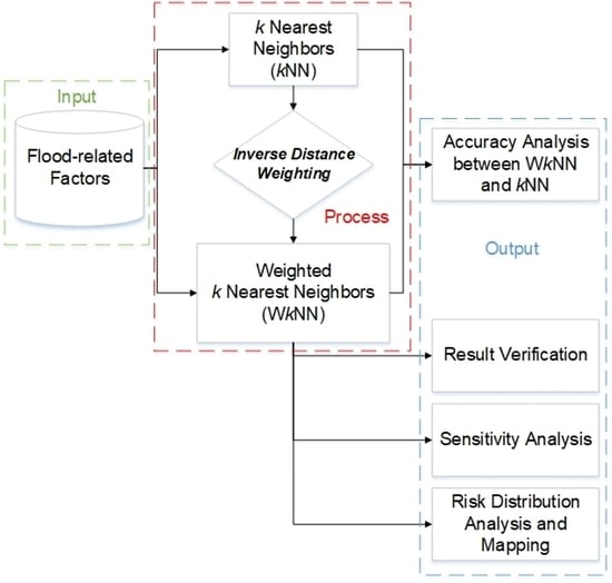
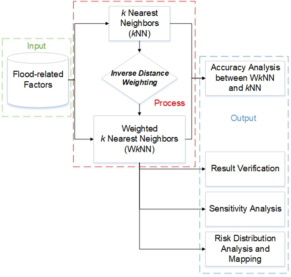
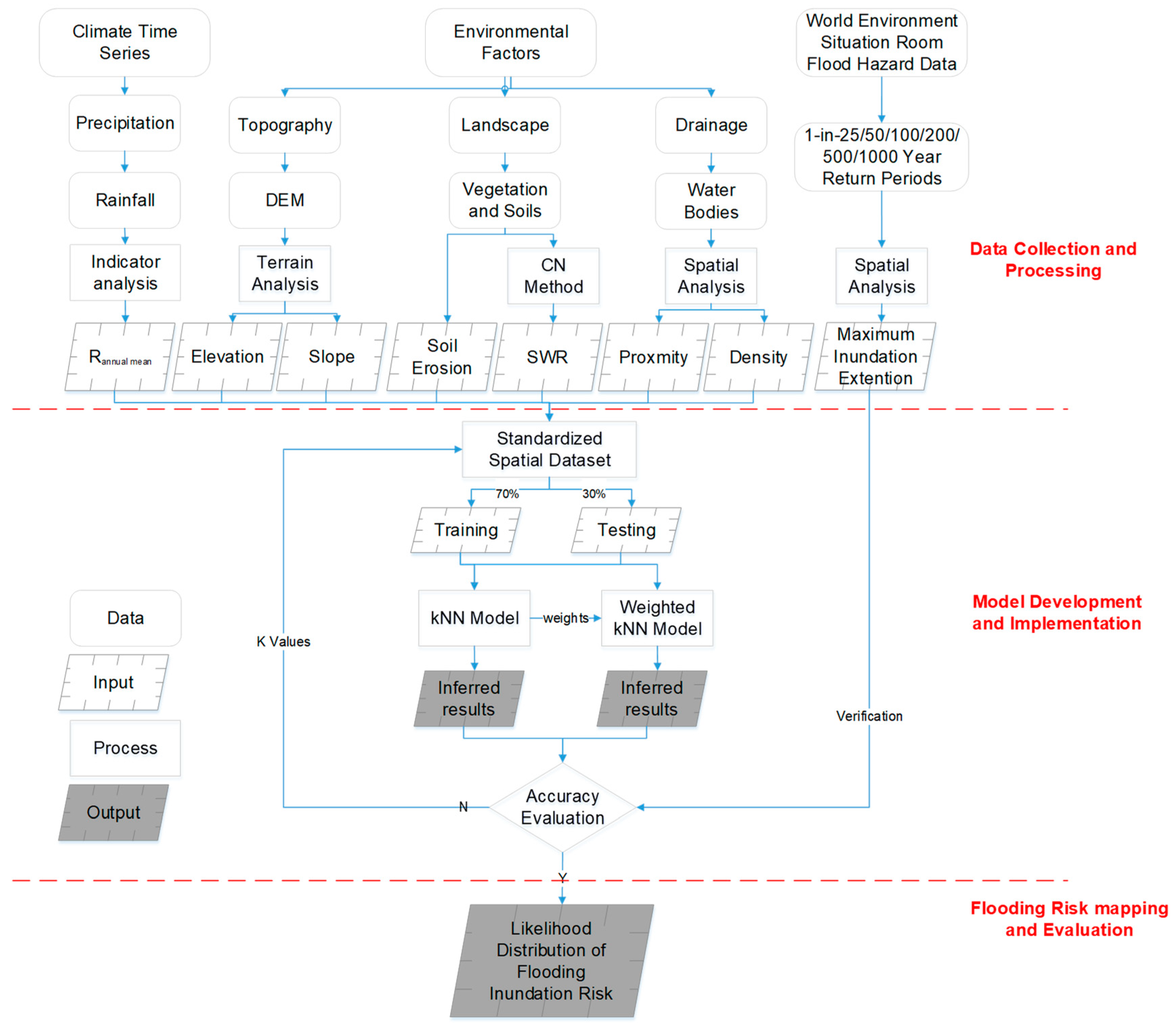
2.3. Framework Conceptualization

After summarizing similar research investigations, a WkNN-based spatial framework of an FIR assessment for coastal tourism is conceptualized and constructed. The framework can be divided into three parts: data collection (input), model construction (process), and classification and evaluation (output) (Figure 1).

The first module mainly collects spatiotemporal data and flood-related index derivation. The data consists of three spatial branches: climate, environment, and validation data. Several indexes are derived from the flood-induced factors, which range from the mean annual rainfall to the drainage density. The flood hazard data of different year return periods (YRPs) are collected to create the Maximum Inundation Extension (MIE) with historical inundated times, which verifies the evaluation results of the WkNN model.

The second module is the center part of the framework. Following data collection, all spatial indexes are standardized into datasets with four categories: very low risk, low risk, medium risk, and high risk. The standardized datasets within the extent of the MIE are divided into two parts: 70% is the training dataset and 30% is the testing dataset [41]. This is not an inflexible rule. It can vary depending on the size of the dataset and the problem. Usually, the larger portion of the data is allocated to training because the model needs to learn from a significant amount of information. A larger training set can help the model to capture the underlying patterns and relationships in the data.

KNN and WkNN are employed to calculate the categories of random records from training datasets with nearby $k$-training datasets. The inferred results are compared with their existing categories in the training dataset, which produces a confusion matrix and overall accuracy (OA). The WkNN model with the highest OA value will be extended to whole areas. A sensitivity analysis is conducted to explore the relationship between the inputs and outputs of the model.

The third model is used to map and evaluate the likelihood of the FIR and to assess the tourism facilities that are exposed in the FIR.

3. Case Study

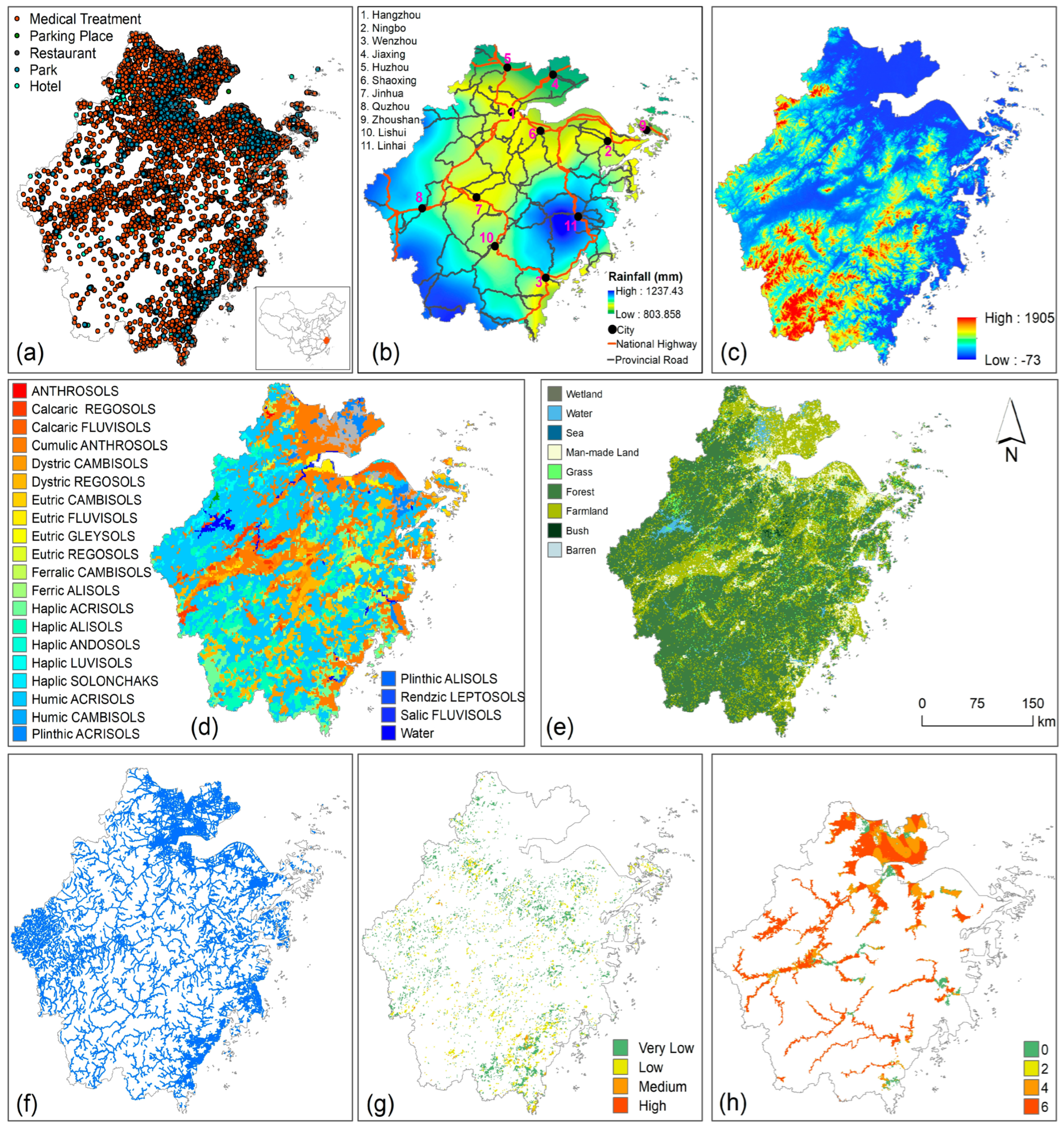
3.1. Study Area

Zhejiang province (118–122.2$°$ E, 27–31.2$°$ N), China was selected as a case study. The province sits on the southeast coast of the Yangtze River Delta and at the land-and-sea junction. It faces the East China Sea and slopes from southwest to northeast [15,42]. In the area, about 74.63% of the area is occupied by mountains and hills, in which relatively steep terrain and extreme precipitation will easily cause flood inundation with the limitation of river flows and fast water accumulation [43]. Moreover, the whole area is deeply affected by a subtropical monsoon climate, which brings heavy rainfall between June and October. Its eastern area is especially frequently impacted by typhoons, which regularly originate between June and October [44]. This period happens to be the best tourist season in Zhejiang and China, which is heavily and widely influenced by the wet season [45,46,47].

The superior location and special environment make it spread superior tourism resources (e.g., West Lake) (Figure 2a) over 11 main cities (Figure 2b), which attract millions of domestic and foreign tourists every year. In 2014, its tourism income occupied 15.7% (about RMB 630 billion) of the provincial GDP (about RMB 4015 billion). However, Zhejiang also experienced a higher FIR, caused by sea levels, typhoons, and tropical cyclones due to complex environmental conditions under risky climate change.

Historical records show that typhoons and tropical cyclones brought heavy rainfall and floods over the study area during the past 60 years from 1950 to 2009, which made the area suffer direct mean annual losses (about RMB 10 billion), especially in its southeast coastal areas. Newspapers are extremely important data sources for data collection and verification. They can be employed as truly historical data records since their reliability and timeliness are relatively high. Therefore, historical flood disaster data for the study between 1950 and 2022 were collected and analyzed from Zhejiang Daily (https://zjrb.zjol.com.cn (accessed on 2 October 2023)). The statistical results show that flood disaster events have negative impacts on Zhejiang province and its tourism facilities. For example, more than 250 and 219 km of roads were washed away by continuous rainfall in Jiaxing City in July 1983. In June 1989, the transmission line in Jingning County was interrupted for 25 h, and two hydropower stations were shut down by rainstorms, causing a temporary shutdown of industries in the county. The highway in the Yunhe area between Jingning and Yunhe collapsed seriously, and houses, warehouses, and shops were flooded by continuous rainfall and floods. In July 1999, more than 900 enterprises ceased production and were semi-suspended, of which 94.6 percent of those with sales revenues of more than RMB 5 million were affected by the flood inundation disaster in Changxing County. In 2006, the Sang Mei super typhoon triggered 153 deaths in Wenzhou, bringing about RMB 11 billion in direct economic losses [14]. In 2013, typhoon-triggering flood inundation affected eight million residents, and it caused about RMB 33 billion of straight financial losses in Ningbo [15]. Additionally, Zhejiang has a 6500 km coastline and its average sea level has risen 98 mm during the past 30 years, and it is projected to speed up under extreme climates with destructive potential. All of them severely influence tourism operations, socioeconomic income, and even people’s lives [42]. Hence, the continually historical flood damage in the area has underscored an urgent need to assess the FIR to manage flood disasters and promote the stable and sustainable development of Zhejiang’s coastal tourism economy.

3.2. Flood-Derived Spatial Data Collection and Processing

Flood risk and evaluation is a comprehensive system, arising from flood hazard, exposure, and disaster-prone environments at a particular location [18]. The criteria from the three parts have been systematically selected and derived in light of their influences on the occurrence and distribution of flood inundation with domain knowledge [21,48,49]. Flood hazard is defined as a deriving factor for the FIR, such as extreme rainfall. Exposure refers to the degree or extent of persons, environments, or assets (e.g., tourism facilities) that are likely to be located in flood-prone areas. Other factors, including topography, hydrology, land use, and soil, are defined as disaster-prone environments. They were extracted and standardized via data processing and analysis in a GIS environment, and all of these factors worked as spatial inputs for the WkNN-centered framework to reason the FIR in the future.

3.2.1. Rainfall

Rainfall is a direct factor and has a significant impact on the occurrence and distribution of flood inundation. It can commonly be divided into two main types: short-period intensive rainfall and prolonged extensive rainfall. Due to the limitation of data in some countries, such as China, this study extracts the annual mean precipitation, which has a notable influence on flood events [50], from Asian Precipitation—Highly Resolved Observational Data Integration Towards Evaluation (APHRODITE) (at 25 km resolution) between 1951 and 2007 as rainfall indices [51]. The APHRODITE has been illustrated to match the accurate features of rain belts in China [31,52,53]. The extracted APHRODITE dataset was interpolated into gridded rainfall data with Inverse Distance Weighting and clipped within the study area in ArcGIS version 10.4 [54] (Figure 2b and Figure 3a).

3.2.2. Topographic Features

Topography is the key driver for flood formation and redistribution (Figure 2c). Generally, a lower area has a fairly higher flood risk since it can easily be inundated by surrounding water. Instead, a higher area has a better drainage capacity. In this study, two indices were extracted to represent topography. They are elevation (Figure 3b) and slope (Figure 3c) [55]. Elevation is the height above a fixed reference point, regularly the mean sea level. The area with a lower elevation is easily inundated by flood water from higher ones, and vice versa [31]. Slope is the steepness or the degree of incline of a surface. A steeper surface has a lower likelihood of flood inundation since water easily runs to low-lying land. Both indices were produced from DEM at a 30 m resolution from the United States Geological Survey (https://earthexplorer.usgs.gov (accessed on 15 February 2023)) and Geospatial Data Cloud in China (https://www.gscloud.cn/sources/index?pid=302 (accessed on 18 February 2023)).

3.2.3. Soil Water Retention (SWR)

Soil water retention affects the rate at which water can infiltrate the ground. Different types of soil have diverse capacities to hold or infiltrate water, which are mutually determined by the soil porosity and vegetation on the surface. Usually, drier soil caused by lengthy and terrible droughts needs more water to bring about flood inundation, but moist or wet surfaces are more easily prone to accumulate flood water. Meanwhile, the probability of flood hazards decreases with an increase in soil infiltration [54]. In flood investigations, the soil infiltration rates can be reflected by the Hydrologic Soil Group (HSG). It can be further classified into four subgroups based on the infiltration rates. Group A has the highest rate under sandy characteristics, such as sandy loam. Subgroup D has the lowest infiltration rates and clay features, such as silty clay or clay. Group B and Group C have moderate to slow rates, which consist of (silt) loam and sandy clay loam.

The soil storage indicates the amount of water that is stored in the soil, which decides the occurrence of flood inundation. The potential maximum Soil Water Retention (SWR) can reflect how much water is in the soil, and it can be calculated with a hydrological modeling method that is driven by the Soil Conversation Service Curve Number (SCS-CN) [56,57]. The SCS-CN values were jointly calculated using hydrological features, the soil type (Figure 2d), and land use (Figure 2e,

Table 1. CN values under soil type.

Soil Type	A	B	C	D
Farmland	72	82	88	92
Forest	36	60	73	79
Grass	39	61	74	80
Bush	36	60	74	80
Wetland	32	58	72	79
Man-made land	89	92	94	95
Barren	72	82	88	90
Water	100	100	100	100

) [58], and they were referenced from the list of Soil Conservation Service [59]. The CN values can be calculated by intersecting the HSG, soil type, and land cover. Based on the CN approach, the SWR (Figure 3d) in cells can be calculated by using

$${SWR}_i={SWR}_0 (\frac{100}{{CN}_i}-1)$$

(5)

where ${CN}_i\in (0,100)$ is the CN value of an $i\mathrm{t}\mathrm{h}$ cell, and ${SWR}_0$ = 254 for units of millimeters.

3.2.4. Drainage System

A drainage system (Figure 2f) needs to be considered in the FIR since it determines the formation and distribution of flood inundation. Occasionally, overflowing floods may happen over banks in drainage systems such as rivers under extreme rainfall. Frequently, two main indices of drainage systems determine the distribution of flood inundation on the earth’s surface. They are the drainage proximity (Figure 3e) and drainage density (Figure 3f). The proximity denotes the distance to the nearest rivers or other water bodies, and the drainage density refers to the lengths of rivers per unit area. Based on our previous research [31], the areas near drainage networks within 200 m are assigned as areas with a high FIR, and the risk level decreases with the increase in distance [60]. The two factors were attained from the Global River Database with Multiple Buffer operators and the Line Density function using a 1 km radius in a GIS [61,62].

3.2.5. Soil Erosion

Soil erosion has a greater impact on the form and distribution of flood inundation, which can increase the risk of flood inundation [63] since soil erosion can remove the topsoil layer, which is often the most fertile and porous part of the soil. When this layer is lost, the soil’s ability to absorb and retain water is diminished. As a result, during rainfall events, water is more likely to run off the surface rather than infiltrate into the ground. This increased runoff can contribute to flash floods and more significant flood events. Soil erosion refers to the natural process of soil being moved from one location to another by natural environmental factors (e.g., water) and human activities such as deforestation, overgrazing, and improper agricultural practices [64]. Under the same rainfall conditions, areas with severe soil erosion are much more likely to be inundated by flood inundation than areas with well-preserved surface vegetation since a bare surface has a lower capacity to control water. In this study, soil data at a 1 km resolution were accessed from the Geographical Information Monitoring Cloud Platform (http://www.dsac.cn (accessed on 21 February 2023)) and processed in ArcGIS 10.4 (Figure 2g and Figure 3g).

3.2.6. Detection of Maximum Inundation Extent

Remote Sensing (RS) has been applied in many flood-related investigations for many years. Its images are more easily acquired, but they have some restrictions. For instance, Moderate Resolution Imaging Spectroradiometers (MODIS) have higher temporal resolutions but lower spatial resolutions (500 m), and they are commonly negatively affected by cloud cover, which may cause them to miss out on flash rainfall events and corresponding flood disasters. Necessarily, other spatial data sources should be found to replace RS images in the FIR. The World Environment Situation Room platform (WESR, https://wesr.unepgrid.ch/?project=MX-XVK-HPH-OGN-HVE-GGN&language=en (accessed on 24 February 2023)) delivers practicable replacements for the FIR. It provides global dynamic data and systematic tools from different sources, as well as visualization tools that enable users to interact with and explore the data online [65]. It also assists users in observing and analyzing environmental issues and trends and in formulating effective environmental policies and protections. WESR products have been illustrated and employed in scientific investigations in data-scarce regions as well as in developing countries, which can be extremely helpful in increasing the preparedness and awareness of the population and reducing catastrophic impacts [66]. In the flood risk field, the WESR provides six Year Return Periods (YRPs) at 1 km resolution. They are 1-in-25, 1-in-50 (Figure 2h), 1-in-100, 1-in-200, 1-in-500, and 1-in-1000 YRPs. All data were cross-checked with satellite flood footprints from various data sources and showed high accuracy. The values of cells in YRP maps were reassigned again if a cell value was greater than 0, they were assigned as 1; otherwise, they were assigned as 0. The reassigned maps were overlaid to derive an inundation frequency map as a Maximum Inundation Extension (MIE; Figure 3j). In MIE, the cell values range from 0 to 6, representing a very low risk to a high risk. High risk means extremely vulnerable and frequent inundation from 1-in-25 to 1-in-1000 YPR floods. MIE was selected as the reference imagery to verify the inferred maps derived from kNN and WkNN.

3.2.7. Criteria Standardization

To improve the efficiency of the calculation, all of the spatial input data were converted into 1 to 4, which represent a very low risk to a high risk using specific values (Figure 3a–g). There are many methods used to standardize the criterion indices, such as domain knowledge and Natural Breaks (Jenks). In this study, all input criteria were standardized using Natural Breaks (Jenks) method in ArcGIS and R programming. Natural Breaks (Jenks) refers to divisions or cutoff points in data that occur naturally or intuitively, based on the characteristics of the data, and it is well employed in the FIR [28,29]. In addition, all spatial datasets were then projected, resampled to 1 km grid cells, clipped to the study area, and registered, so all input grids accurately overlaid with the same projection, cell size, and extent.

4. Results and Discussion

A flood risk map was plotted as a derived result of the spatial evaluation framework for the FIR. The flood risk was divided into four levels: high risk (red), medium risk (orange), low risk (yellow), and very low risk (green).

4.1. Result Verification

The innovative WkNN-based spatial framework effectively produced the spatial distribution of the FIR for the whole study area. To validate the evaluation accuracy (EA) of the WkNN model, an accuracy comparison was conducted between the spatially inferred results (Figure 3k) extracted from Figure 3h against the MIE (Figure 3j). Overall, 80.59% of the WkNN results reasonably confirmed the actual MIE, where the cell value > 0. Among the matched areas, 80.14%, 90.13%, 65.50%, and 84.14% of the predicted categories in the WkNN area (Figure 3k) were well matched with the MIE area (Figure 3j) in high, medium, low, and very low risk, respectively. This reflects that the WkNN results (Figure 3h) are sound and reasonable. The remaining mistakes could be explained by the uncertainties and a little bit of inaccuracy in the WESR data in certain areas. Moreover, it should be noted that the predicted risk extent is larger than the WESR data. The reason for this may be that the extension of the WESR data is insufficient, which can be vividly shown in the empty circle in the northeast area, and some areas do not have data (Figure 3j).

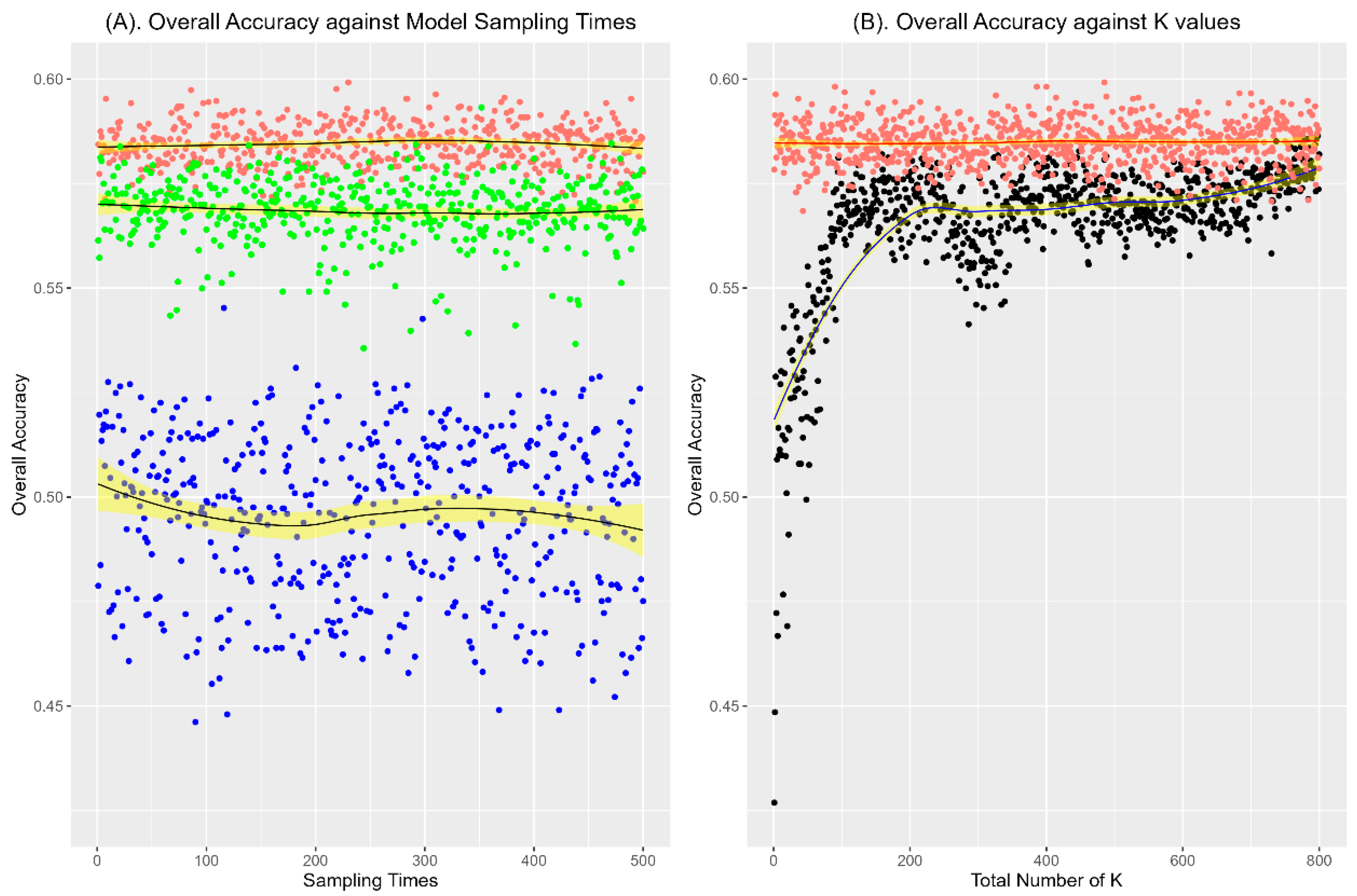
4.2. Sensitivity Analysis

A sensitivity analysis is essential to explore the relationships between the inputs and outputs of models, which can picture the performances, structures, and uncertainty of models. For WkNN-based models, the sampling datasets and the $k$ values determine the EA of models and inferred outcomes.

4.2.1. Sensitivity Analysis in Relation to Sampling Times

This study explored the relationship between sampling times and the tendency of EA under $k$ values. The overall accuracy (OA) was chosen to evaluate the performances of kNN and W$k$NN against the MIE. The OA denotes the proportion of correct predictions made by models or systems over the total number of predictions [67,68], which can directly reflect the EA, and it is easy to understand and use. Figure 4A shows that the larger the k value, the higher the OA accuracy since the EA curve distribution of blue points ($k$ = 5) is significantly lower than the EA curve distribution of green points ($k$ = 95). The 5 and 95 values were selected randomly and are roughly equal to the square root of the training datasets, respectively (8947) [38]. Under different sampling times (from 1 to 500), the range of both OAs (in blue and green) is relatively larger, which shows that the kNN method is unstable. However, compared with kNN, the WkNN method (in red) shows comparative robustness since the OA range of the WkNN model is aggregated around the medium value (about 0.58) when taking the same $k$ values ($k$ = 5 and $k$ = 95), which additionally demonstrates that the predicted performance of WkNN is higher than that of kNN.

4.2.2. Sensitivity Analysis in Relation to $k$ Values

K values play key roles in model performance. An appropriate $k$ value determines the robust and predicted results of the kNN models. Conversely, inappropriate $k$ values will cause the problem of bias-various tradeoffs [38]. Therefore, this study explored and compared the performances and influences of $k$ values in kNN and WkNN and selected the optimal $k$ values (the highest value in the OA) to infer the FIR for the whole study area. In this study, the range of $k$ values from 1 to 800 covers the square root (95 and 315) of the observations (8947) and the whole study dataset (98,709). The results show that the OA of kNN, which ranges from 0.43 to 0.58, is lower than the OA of WkNN, which ranges from 0.57 to 0.60. Similarly, the trend in the EA of WkNN is reasonably stable than that of kNN. Overall, the OA increases with the growth of $k$ values, particularly, and it shows non-linear increases when the $k$ values are between 1 and 200 (Figure 4B). When the $k$ values are between 200 and 400, the OA presents a declining trend, but after 400, the value of the EA increases slowly. All of these demonstrate that the $k$ values have significant impacts on kNN and WkNN, but the latter performs more robustly.

4.3. Comparison of WkNN with kNN

The evaluation results of WkNN (Figure 3h) using Equation (4) were demonstrated using a comparison with those of a published spatial-based kNN method (Figure 3i) [31] using Equation (1). The comparison shows that WkNN is better than kNN, such as in sampled areas 1 to 3, because their results are more similar to the reference MIE (Figure 3j) in visualization. Also, three areas were sampled in the north (area 4 in a grey rectangle), west (area 5 in a blue rectangle), and southeast (area 6 in a purple rectangle) to compare the evaluation accuracy (EA) between WkNN (Figure 3k) and kNN (Figure 3l) against the MIE (Figure 3j). Area 4 shows that the inferred WkNN’s results accurately match the pattern of the MIE with values of >0. However, kNN shows opposite results in some areas, which means there is a high risk in the MIE, but a low risk or even very low risk is in the kNN results. These mismatches have also occurred in other regions, such as in areas 5 and 6. All of these reflect that the WkNN method has a higher prediction accuracy than kNN.

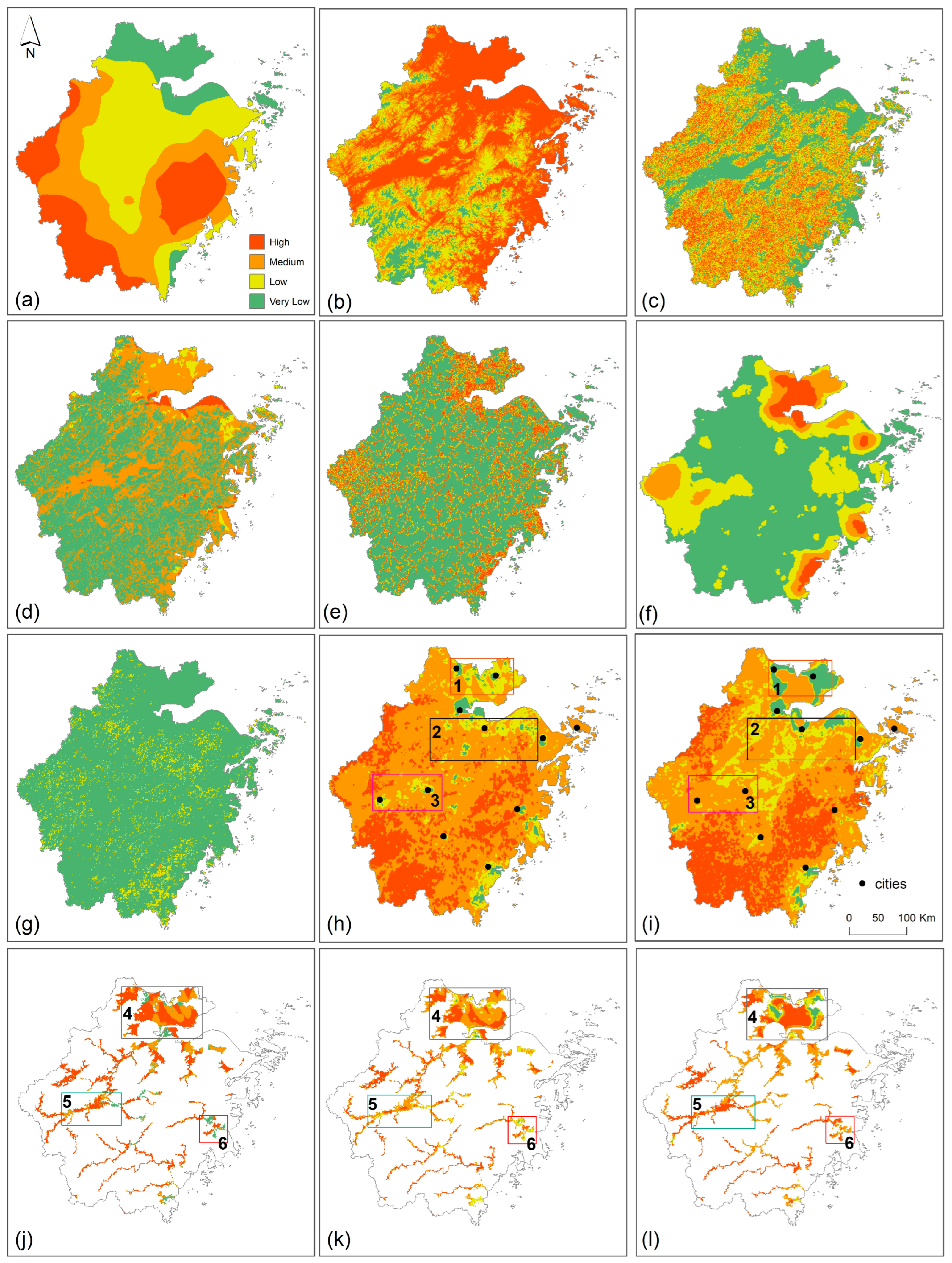
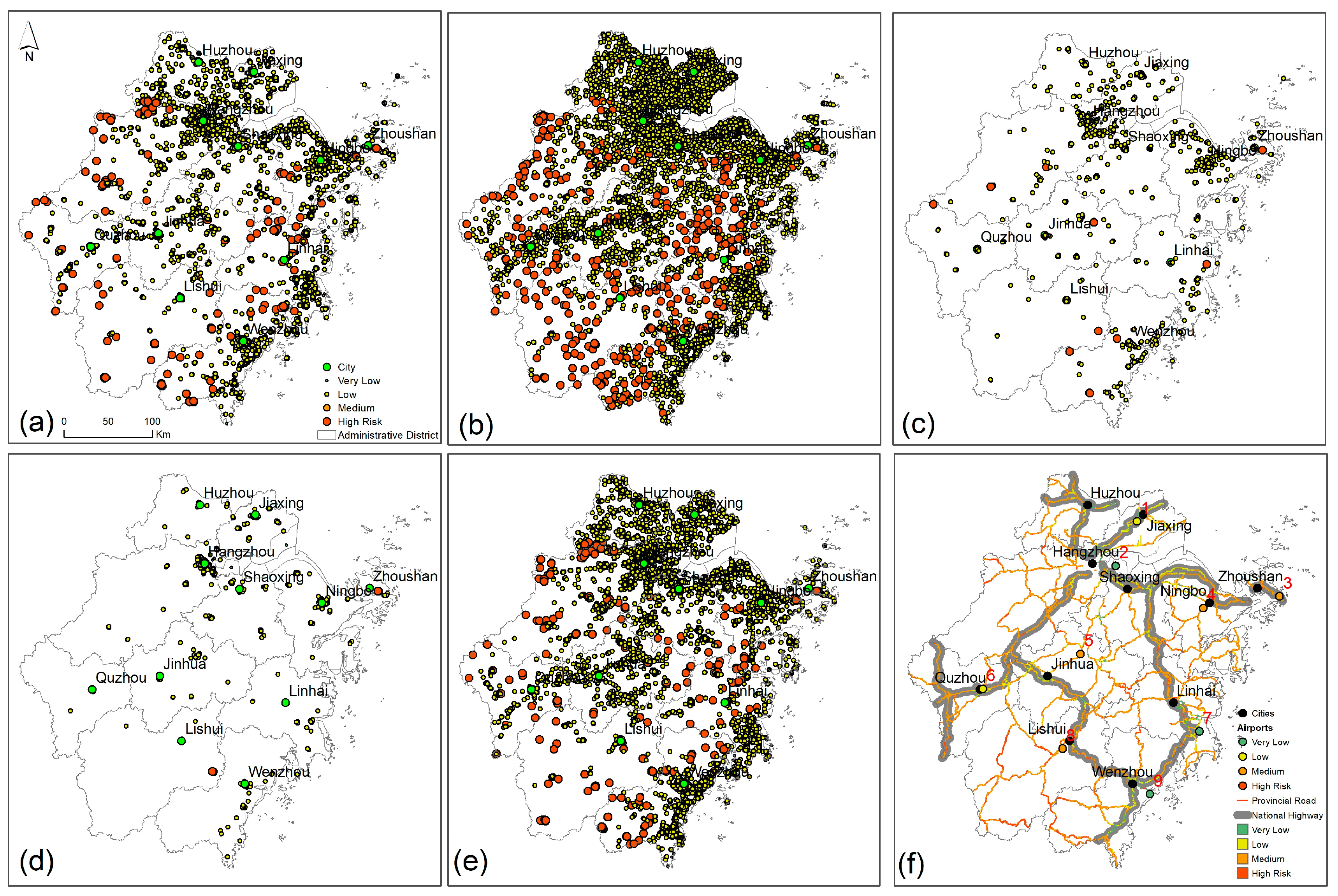
4.4. Risk Distribution Analysis

The resulting map (Figure 3h) illustrates the extent and distribution of the FIR in the whole study area. The statistics of each flood category from high risk to very low risk were conducted, which demonstrates that about half of the area is classified as medium-high FIR risk. Around 2.85% of the whole area is covered by high risk, 64.83% is medium risk, 10.8% is low risk, and 21.52% is very low risk. High-risk areas can be observed, particularly in the southwestern area that is affected by elevation (57.63 km²) and precipitation (36.13 km²). The result further demonstrates that elevation is the key factor in the form and redistribution of flooding inundation. Elevation can contribute to flash flooding in mountainous regions. Heavy rainfall or rapid rainstorms at higher elevations can lead to the sudden release of large volumes of water downstream, causing flash floods in lower-lying areas. Meanwhile, heavy rainfall over a short period can overwhelm the capacity of rivers and stormwater systems to handle the water, leading to flash floods. Moreover, high-risk areas are scattered across the eastern part, which is heavily affected by slope (about 32.77 km²) and SWR (about 24.86 km²). In areas with a steep slope, such as mountainous or hilly regions, water flows downhill more rapidly. When heavy rainfall occurs in these areas, the water can quickly run off the slopes and accumulate in lower-lying regions, potentially causing flash floods. The steepness of the terrain can lead to a high runoff speed and increased water volume downstream. Soils with high water retention, such as clay soils in the study area, may have slower infiltration rates. This can lead to increased surface run-off during heavy rainfall events, which may contribute to flash flooding if the rainfall rate exceeds the soil’s infiltration capacity.

In the northern area, there is also a high-risk area under lower evaluation. Most areas are covered by medium risk in flood inundation, which is larger than high risk, since compared with medium flood risk, high flood risk rarely happens, unless there are extraordinary climate events and fragile environments, such as extreme rainfall and bare ground. A medium risk is mutually affected by multiple factors over the center area. Elevation (152.55 km²) and precipitation (76.84 km²) contribute greatly to the central part across the west to the east. In the fringe of the study area, medium risk is mainly affected by the drainage density and proximity. The high-medium area demonstrates that elevation and precipitation are the two extremely important factors for the FIR. Slope, erosion, and proximity make similar contributions to high-medium risk since their areas are 32.77 km² and 73.45 km² in high risk and medium risk, separately. The river density and SWR have little contribution to high-medium FIR. Based on prior experience [49], a high density of rivers or areas nearer to the rivers should have high or medium flood risks, but actually, these areas have low or very low flood risks in the study. This is mainly because drainage systems carry more flood into the sea and mitigate the stress of flood inundation pressure in the study area. Also, larger cities, such as Hangzhou, are mainly located in low-risk or very-low-risk areas, which vividly demonstrates that man-made water conservancy facilities play a huge role in protecting socioeconomic development and alleviating flood risk.

Figure 5 shows the tourism facilities that are exposed in the predicted FIR. To highlight tourism facilities with high-medium risk levels, the facilities with higher risk levels will have bigger point sizes. This illustrates that in most inland areas, some tourism facilities are located in high-medium-risk areas of flood inundation, especially hotels (Figure 5a), medical treatment institutions (Figure 5b), and restaurants (Figure 5e). This is because high-risk areas are often scenic and attractive due to their proximity to water bodies, such as rivers, lakes, or the ocean. Some flood-prone areas may have historical or cultural significance, such as old towns or heritage sites. All of these factors determine that the number of medical treatment institutions is higher than other facilities in high-risk areas for responding to disaster relief and rescue. Therefore, it can easily be understood that medical facilities in high-risk areas will play key roles in effectively mitigating or even preventing the negative impact of flood inundation on tourism facilities and in saving lives. Additionally, parks (Figure 5c) and parking places (Figure 5d) are mainly located in low-risk or very-low-risk areas since most of them are in urban areas. Additionally, the study area has a wonderful road system (Figure 5f) at the national-provincial levels. The majority of roads are located in medium- or low-risk areas of flood inundation, which not only helps to develop tourism resources but also helps to efficiently carry out disaster relief and post-disaster reconstruction.

Airports play important roles in modern tourism, such as providing an easier way for tourists to travel and increasing tourist arrivals. In the study area, although airports are impacted by flood inundation, most of them are located in low or very low FIR areas (Figure 5f). There are only four airports covered by a medium FIR, including Zhoushan Putuoshan Airport (Number 3), Ningbo LiShe International Airport (Number 4), Yiwu Airport (Number 5), and Lishui Airport (Number 8), since these airports are located in medium-high-risk areas with high risks of precipitation, elevation, and SWR. Two airports, Jiaxing Nanhu Airport (Number 1) and Quzhou Airport (Number 6) are located in low FIR areas. The other three airports, Hangzhou Xiaoshan International Airport (Number 2), Taizhou Luqiao Airport (Number 7), and Wenzhou Longwan International Airport (Number 9), are situated in very low-risk areas. These airports in low- or very-low-risk areas are of great importance in evacuating passengers in the case of flood inundation disasters under extremes.

Notably, most tourism facilities in coastal cities are in low- or very-low-risk areas, especially from the Hangzhou-centered northern coastal areas to the southern Wenzhou areas. Figure 3h and Figure 5 demonstrate that tourist facilities and road infrastructure are at a low-risk level in the cities and nearby areas. This illustrates that local departments have conducted a lot of practical and efficient work on disaster prevention and mitigation in coastal flood-prone areas. This can prove that engineering measures play key roles in protecting socioeconomic activities, including tourism, which can provide a valuable reference for the vast coastal areas around the world.

5. Conclusions

This study develops an innovative spatial framework, which integrates Weighted kNN (WkNN), Geographic Information Systems (GISs), and other flood-relative indices to infer, map, and evaluate the distribution of the Flood Inundation Risk (FIR) for tourism. It was illustrated using a Chinese case study, particularly of Zhejiang province, where the flood inundation risk is highly related to environmental variabilities and extreme weather events, such as typhoons, which bring about long-term or intensive rainfall. All of these environmental criteria from rainfall to soil have diverse and complicated contributions to flood hazards. The WESR was used as the predicted result validation for tourism in the FIR for the first time. The improved WkNN was developed based on the traditional kNN method, combined with GIS, and employed in the FIR assessment. In WkNN, the weights were calculated as inversely proportional to the distance between the query points and their k nearest neighbors. A GIS was used as a spatial tool to derive flood-influenced indices and process the number of spatial factors with multitemporal and multispatial resolution from different sources. The evaluation results show that precipitation and elevation make huge contributions to high-medium risk, and drainage systems positively alleviate the regional stress of the FIR.

The WkNN-based framework was effectively carried out in the case study and obtained reasonable outcomes, which further demonstrated that WkNN is superior to kNN in the evaluation accuracy (EA) and flood risk analysis. Meanwhile, $k$ values are still significant parameters for kNN and WkNN. Suitable $k$ values will improve the performances of models in the EA. The WkNN outcomes can match the WESR data well, which can deliver the fundamentals for flood disaster prevention and mitigation for tourism in a coastal area and assist decision makers in adopting effective measures to prevent and mitigate the negative impacts of flood disasters.

The innovative spatial framework was programmed and repeatable with GIS, R, and Python programming, which can be flexibly used in other disaster-related investigations, and they are also not limited by the number of model inputs. The evaluation results will make corresponding changes responsive to different input indices. However, there are some limitations that this study did not consider. For example, due to the limitation of data sources, this study did not fully use Remote Sensing imagery, such as Synthetic Aperture Radar, in the flood risk assessment. Additionally, this study did not assess the adverse economic consequences of flooding on the tourism industry. As a further step, we plan to probe deeply into these fields and provide more precise assessments.

References

- Papageorgiou, M. Coastal and marine tourism: A challenging factor in Marine Spatial Planning. Ocean Coast. Manag. 2016, 129, 44–48. [Google Scholar] [CrossRef]
- Chen, Y.H.; Kim, J.; Mueller, N. Estimating the economic impact of natural hazards on shared accommodation in coastal tourism destinations. J. Destin. Mark. Manag. 2021, 21, 100634. [Google Scholar] [CrossRef]
- Lithgow, D.; Martínez, M.L.; Gallego-Fernández, J.B.; Silva, R.; Ramírez-Vargas, D.L. Exploring the co-occurrence between coastal squeeze and coastal tourism in a changing climate and its consequences. Tour. Manag. 2019, 74, 43–54. [Google Scholar] [CrossRef]
- Perles-Ribes, J.F.; Ramón-Rodríguez, A.B.; Moreno-Izquierdo, L.; Such-Devesa, M.J. Machine learning techniques as a tool for predicting overtourism: The case of Spain. Int. J. Tour. Res. 2020, 22, 825–838. [Google Scholar] [CrossRef]
- Junqing, H.; Han, T.; Jiawei, H.; Yanting, M.; Xinxiang, J. Impacts of risk perception, disaster knowledge and emotional attachment on tourists’ behavioral intentions in Qinling Mountain, China. Front. Earth Sci. 2022, 10, 880912. [Google Scholar]
- Morsy, M.; Sayad, T.; Khamees, A.S. Towards instability index development for heavy rainfall events over Egypt and the Eastern Mediterranean. Meteorol. Atmos. Phys. 2019, 132, 255–272. [Google Scholar] [CrossRef]
- Zhang, Y.; Wang, Y.; Chen, Y.; Xu, Y.; Zhang, G.; Lin, Q.; Luo, R. Projection of changes in flash flood occurrence under climate change at tourist attractions. J. Hydrol. 2021, 595, 126039. [Google Scholar] [CrossRef]
- Vitousek, S.; Barnard, P.L.; Fletcher, C.H.; Frazer, N.; Erikson, L.; Storlazzi, C.D. Doubling of coastal flooding frequency within decades due to sea-level rise. Sci. Rep. 2017, 7, 1399. [Google Scholar] [CrossRef]
- Lyu, H.M.; Wang, G.F.; Cheng, W.C.; Shen, S.L. Tornado hazards on June 23 in Jiangsu Province, China: Preliminary investigation and analysis. Nat. Hazards 2016, 85, 597–604. [Google Scholar] [CrossRef]
- Kundzewicz, Z.W.; Su, B.; Wang, Y.; Wang, G.; Wang, G.; Huang, J.; Jiang, T. Flood risk in a range of spatial perspectives—From global to local scales. Nat. Hazards Earth Syst. Sci. 2019, 19, 1319–1328. [Google Scholar] [CrossRef]
- Sun, S.; Zhai, J.; Li, Y.; Huang, D.; Wang, G. Urban waterlogging risk assessment in well-developed region of Eastern China. Phys. Chem. Earth Parts A/B/C 2020, 115, 102824. [Google Scholar] [CrossRef]
- Fang, J.; Zhang, C.; Fang, J.; Liu, M.; Luan, Y. Increasing exposure to floods in China revealed by nighttime light data and flood susceptibility mapping. Environ. Res. Lett. 2021, 16, 104044. [Google Scholar] [CrossRef]
- Kumar, M.D.; Tandon, S.; Bassi, N.; Mohanty, P.K.; Kumar, S.; Mohandas, M. A framework for risk-based assessment of urban floods in coastal cities. Nat. Hazards 2021, 110, 2035–2057. [Google Scholar] [CrossRef]
- Lu, Y.; Ren, F.; Zhu, W. Risk zoning of typhoon disasters in Zhejiang Province, China. Nat. Hazards Earth Syst. Sci. 2018, 18, 2921–2932. [Google Scholar] [CrossRef]
- Liang, H.; Zhou, X. Impact of tides and surges on fluvial floods in coastal regions. Remote Sens. 2022, 14, 5779. [Google Scholar] [CrossRef]
- Thaler, T.; Seebauer, S. Bottom-up citizen initiatives in natural hazard management: Why they appear and what they can do? Environ. Sci. Policy 2019, 94, 101–111. [Google Scholar] [CrossRef]
- Cronin, S.J.; Gaylord, D.R.; Charley, D.; Alloway, B.V.; Wallez, S.; Esau, J.W. Participatory methods of incorporating scientific with traditional knowledge for volcanic hazard management on Ambae Island, Vanuatu. Bull. Volcanol. 2004, 66, 652–668. [Google Scholar] [CrossRef]
- Lai, X.; Wen, J.; Shan, X.; Shen, L.; Wan, C.; Shao, L.; Wu, Y.; Chen, B.; Li, W. Cost-benefit analysis of local knowledge-based flood adaptation measures: A case study of Datian community in Zhejiang Province, China. Int. J. Disaster Risk Reduct. 2023, 87, 103573. [Google Scholar] [CrossRef]
- Mendelsohn, R.; Emanuel, K.; Chonabayashi, S.; Bakkensen, L. The impact of climate change on global tropical cyclone damage. Nat. Clim. Chang. 2012, 2, 205–209. [Google Scholar] [CrossRef]
- Baade, R.A.; Baumann, R.; Matheson, V. Estimating the economic impact of natural and social disasters, with an application to hurricane katrina. Urban Stud. 2016, 44, 2061–2076. [Google Scholar] [CrossRef]
- Chen, Y.; Liu, R.; Barrett, D.; Gao, L.; Zhou, M.; Renzullo, L.; Emelyanova, I. A spatial assessment framework for evaluating flood risk under extreme climates. Sci. Total Environ. 2015, 538, 512–523. [Google Scholar] [CrossRef] [PubMed]
- Tsai, C.H.; Chen, C.W. Development of a mechanism for typhoon- and flood-risk assessment and disaster management in the hotel industry—A case study of the hualien area. Scand. J. Hosp. Tour. 2011, 11, 324–341. [Google Scholar] [CrossRef]
- Sealy, K.S.; Strobl, E. A hurricane loss risk assessment of coastal properties in the caribbean: Evidence from the Bahamas. Ocean Coast. Manag. 2017, 149, 42–51. [Google Scholar] [CrossRef]
- Shi, Y.; Wen, J.; Xi, J.; Xu, H.; Shan, X.; Yao, Q.; Xia, J. A study on spatial accessibility of the urban tourism attraction emergency response under the flood disaster scenario. Complexity 2020, 2020, 9031751. [Google Scholar] [CrossRef]
- Erena, S.H.; Worku, H.; De Paola, F. Flood hazard mapping using FLO-2D and local management strategies of Dire Dawa city, Ethiopia. J. Hydrol. Reg. Stud. 2018, 19, 224–239. [Google Scholar] [CrossRef]
- Yildirim, E.; Demir, I. An integrated web framework for HAZUS-MH flood loss estimation analysis. Nat. Hazards 2019, 99, 275–286. [Google Scholar] [CrossRef]
- Chen, Y.; Wang, Y.; Zhang, Y.; Luan, Q.; Chen, X. Flash floods, land-use change, and risk dynamics in mountainous tourist areas: A case study of the Yesanpo Scenic Area, Beijing, China. Int. J. Disaster Risk Reduct. 2020, 50, 101873. [Google Scholar] [CrossRef]
- Liu, R.; Chen, Y.; Wu, J.; Gao, L.; Barrett, D.; Xu, T.; Li, X.; Li, L.; Huang, C.; Yu, J. Integrating entropy-based naive Bayes and GIS for spatial evaluation of flood hazard. Risk Anal. 2017, 37, 756–773. [Google Scholar] [CrossRef]
- Liu, R.; Chen, Y.; Wu, J.; Gao, L.; Barrett, D.; Xu, T.; Li, L.; Huang, C.; Yu, J. Assessing spatial likelihood of flooding hazard using naïve Bayes and GIS: A case study in Bowen Basin, Australia. Stoch. Environ. Res. Risk Assess. 2015, 30, 1575–1590. [Google Scholar] [CrossRef]
- Stefanidis, S.; Stathis, D. Assessment of flood hazard based on natural and anthropogenic factors using analytic hierarchy process (AHP). Nat. Hazards 2013, 68, 569–585. [Google Scholar] [CrossRef]
- Liu, S.; Liu, R.; Tan, N. A spatial improved-kNN-based flood inundation risk framework for urban tourism under two rainfall scenarios. Sustainability 2021, 13, 2859. [Google Scholar] [CrossRef]
- Liu, K.; Yao, C.; Chen, J.; Li, Z.; Li, Q.; Sun, L. Comparison of three updating models for real time forecasting: A case study of flood forecasting at the middle reaches of the Huai River in East China. Stoch. Environ. Res. Risk Assess. 2016, 31, 1471–1484. [Google Scholar] [CrossRef]
- Liu, K.; Li, Z.; Yao, C.; Chen, J.; Zhang, K.; Saifullah, M. Coupling the k-nearest neighbor procedure with the Kalman filter for real-time updating of the hydraulic model in flood forecasting. Int. J. Sediment Res. 2016, 31, 149–158. [Google Scholar] [CrossRef]
- Cassalho, F.; Beskow, S.; Mello, C.R.; Moura, M.M.; Oliveira, L.F.; Aguiar, M.S. Artificial intelligence for identifying hydrologically homogeneous regions: A state-of-the-art regional flood frequency analysis. Hydrol. Process. 2019, 33, 1101–1116. [Google Scholar] [CrossRef]
- Aryal, S.; Ting, K.M.; Washio, T.; Haffari, G. A comparative study of data-dependent approaches without learning in measuring similarities of data objects. Data Min. Knowl. Discov. 2019, 34, 124–162. [Google Scholar] [CrossRef]
- Rodrigues, É.O. Combining Minkowski and Chebyshev: New distance proposal and survey of distance metrics using k-nearest neighbours classifier. Pattern Recognit. Lett. 2018, 110, 66–71. [Google Scholar] [CrossRef]
- Kutyłowska, M. K-Nearest Neighbours method as a tool for failure rate prediction. Period. Polytech. Civ. Eng. 2017, 62, 318–322. [Google Scholar] [CrossRef]
- Lantz, B. Machine Learning with R: Expert Techniques for Predictive Modeling; Packt publishing Ltd.: Birmingham, UK, 2019. [Google Scholar]
- Malekinezhad, H.; Sepehri, M.; Pham, Q.B.; Hosseini, S.Z.; Meshram, S.G.; Vojtek, M.; Vojteková, J. Application of entropy weighting method for urban flood hazard mapping. Acta Geophys. 2021, 69, 841–854. [Google Scholar] [CrossRef]
- Rahman, A.S.; Rahman, A. Application of principal component analysis and cluster analysis in regional flood frequency analysis: A case study in New South Wales, Australia. Water 2020, 12, 781. [Google Scholar] [CrossRef]
- Batchuluun, G.; Nam, S.H.; Park, K.R. Deep learning-based plant-image classification using a small training dataset. Mathematics 2022, 10, 3091. [Google Scholar] [CrossRef]
- Fang, Y.; Yin, J.; Wu, B. Flooding risk assessment of coastal tourist attractions affected by sea level rise and storm surge: A case study in Zhejiang Province, China. Nat. Hazards 2016, 84, 611–624. [Google Scholar] [CrossRef]
- Li, L.; Li, Z.; He, Z.; Yu, Z.; Ren, Y. Investigation of storm tides induced by super typhoon in Macro-Tidal Hangzhou Bay. Front. Mar. Sci. 2022, 9, 890285. [Google Scholar] [CrossRef]
- Cui, Y.-l.; Hu, J.-h.; Xu, C.; Zheng, J.; Wei, J.-b. A catastrophic natural disaster chain of typhoon-rainstorm-landslide-barrier lake-flooding in Zhejiang Province, China. J. Mt. Sci. 2021, 18, 2108–2119. [Google Scholar] [CrossRef]
- Zhang, W.; Wang, W.; Lin, J.; Zhang, Y.; Shang, X.; Wang, X.; Huang, M.; Liu, S.; Ma, W. Perception, knowledge and behaviors related to typhoon: A cross sectional study among rural residents in Zhejiang, China. Int. J. Environ. Res. Public Health 2017, 14, 492. [Google Scholar] [CrossRef] [PubMed]
- Liao, X.; Xu, W.; Zhang, J.; Qiao, Y.; Meng, C. Analysis of affected population vulnerability to rainstorms and its induced floods at county level: A case study of Zhejiang Province, China. Int. J. Disaster Risk Reduct. 2022, 75, 102976. [Google Scholar] [CrossRef]
- Cao, F.; Xu, X.; Zhang, C.; Kong, W. Evaluation of urban flood resilience and its space-time evolution: A case study of Zhejiang Province, China. Ecol. Indic. 2023, 154, 110643. [Google Scholar] [CrossRef]
- Papaioannou, G.; Vasiliades, L.; Loukas, A. Multi-criteria analysis framework for potential flood prone areas mapping. Water Resour. Manag. 2015, 29, 399–418. [Google Scholar] [CrossRef]
- Xiao, Y.; Yi, S.; Tang, Z. Integrated flood hazard assessment based on spatial ordered weighted averaging method considering spatial heterogeneity of risk preference. Sci. Total Environ. 2017, 599–600, 1034–1046. [Google Scholar] [CrossRef]
- Bezak, N.; Horvat, A.; Šraj, M. Analysis of flood events in Slovenian streams. J. Hydrol. Hydromech. 2015, 63, 134–144. [Google Scholar] [CrossRef][Green Version]
- Yatagai, A.; Kamiguchi, K.; Arakawa, O.; Hamada, A.; Yasutomi, N.; Kitoh, A. APHRODITE: Constructing a long-term daily gridded precipitation dataset for asia based on a dense network of rain gauges. Bull. Am. Meteorol. Soc. 2012, 93, 1401–1415. [Google Scholar] [CrossRef]
- Tao, G.; Lian, X. Study on progress of the trends and physical causes of extreme precipitation in China during the last 50 years. Adv. Earth Sci. 2014, 29, 577. [Google Scholar]
- Feng, L.; Hong, W. Characteristics of drought and flood in Zhejiang Province, East China: Past and future. Chin. Geogr. Sci. 2007, 17, 257–264. [Google Scholar] [CrossRef]
- Ouma, Y.; Tateishi, R. Urban flood vulnerability and risk mapping using integrated multi-parametric AHP and GIS: Methodological overview and case study assessment. Water 2014, 6, 1515–1545. [Google Scholar] [CrossRef]
- Lyu, H.M.; Sun, W.J.; Shen, S.L.; Arulrajah, A. Flood risk assessment in metro systems of mega-cities using a GIS-based modeling approach. Sci. Total Environ. 2018, 626, 1012–1025. [Google Scholar] [CrossRef] [PubMed]
- McCuen, R.H. A Guide to Hydrologic Analysis Using SCS Methods; Prentice-Hall, Inc.: Hoboken, NJ, USA, 1982. [Google Scholar]
- Viji, R.; Rajesh Prasanna, P.; Ilangovan, R. Gis based SCS-CN method for estimating runoff in Kundahpalam watershed, Nilgries District, Tamilnadu. Earth Sci. Res. J. 2015, 19, 59–64. [Google Scholar]
- Cao, B.; Yu, L.; Naipal, V.; Ciais, P.; Li, W.; Zhao, Y.; Wei, W.; Chen, D.; Liu, Z.; Gong, P. A 30 m terrace mapping in China using Landsat 8 imagery and digital elevation model based on the Google Earth Engine. Earth Syst. Sci. Data 2021, 13, 2437–2456. [Google Scholar] [CrossRef]
- SCS. Urban Hydrology for Small Watersheds SCS; Engineering Division, Soil Conservation Service, US Department of Agriculture: Washington, DC, USA, 1986.
- Kazakis, N.; Kougias, I.; Patsialis, T. Assessment of flood hazard areas at a regional scale using an index-based approach and Analytical Hierarchy Process: Application in Rhodope-Evros region, Greece. Sci. Total Environ. 2015, 538, 555–563. [Google Scholar] [CrossRef] [PubMed]
- Strahler, A.N. Quantitative geomorphology of drainage basin and channel networks. In Handbook of Applied Hydrology; McGraw-Hill: New York, NY, USA, 1964. [Google Scholar]
- Andreadis, K.M.; Schumann, G.J.P.; Pavelsky, T. A simple global river bankfull width and depth database. Water Resour. Res. 2013, 49, 7164–7168. [Google Scholar] [CrossRef]
- Li, X.; Wei, X. Analysis of the relationship between soil erosion risk and surplus floodwater during flood season. J. Hydrol. Eng. 2014, 19, 1294–1311. [Google Scholar] [CrossRef]
- Park, S.; Oh, C.; Jeon, S.; Jung, H.; Choi, C. Soil erosion risk in Korean watersheds, assessed using the revised universal soil loss equation. J. Hydrol. 2011, 399, 263–273. [Google Scholar] [CrossRef]
- Jabbour, J.; Caldas, A.; Peduzzi, P. The world environment situation room: Rethinking environmental assessment. AGU Fall Meet. Abstr. 2018, 2018, GH11D-0932. [Google Scholar]
- Dottori, F.; Salamon, P.; Bianchi, A.; Alfieri, L.; Hirpa, F.A.; Feyen, L. Development and evaluation of a framework for global flood hazard mapping. Adv. Water Resour. 2016, 94, 87–102. [Google Scholar] [CrossRef]
- Foody, G.M. Status of land cover classification accuracy assessment. Remote Sens. Environ. 2002, 80, 185–201. [Google Scholar] [CrossRef]
- Liu, C.; Frazier, P.; Kumar, L. Comparative assessment of the measures of thematic classification accuracy. Remote Sens. Environ. 2007, 107, 606–616. [Google Scholar] [CrossRef]