Measuring the Influence of Multiscale Geographic Space on the Heterogeneity of Crime Distribution

Abstract

Urban crimes are not homogeneously distributed but exhibit spatial heterogeneity across a range of spatial scales. Meanwhile, while geographic space shapes human activities, it is also closely related to multiscale characteristics. Previous studies have explored the influence of underlying geographic space on crime occurrence from the mechanistic perspective, treating geographic space as a collection of points or lines, neglecting the multiscale nature of the spatial heterogeneity of crime and underlying geographic space. Therefore, inspired by the recent concept of “living structure” in geographic information science, this study applied a multiscale analysis method to explore the association between underlying geographic space and crime distribution. Firstly, the multiscale heterogeneity is described while simultaneously considering both the statistical and geometrical characteristics. Then, the spatial association rule mining approach is adopted to quantitatively measure the association between crime occurrence and geographic space at multiple scales. Finally, the effectiveness of the proposed methods is evaluated by crime incidents in the city of Philadelphia. Experimental results show that crime heterogeneity is indeed closely related with the spatial scales. It is also proven that the influence of underlying geographic space on crime heterogeneity varies with the spatial scales. This study may enrich the methodology in crime pattern and crime explanation analysis, and it provides useful insights for effective crime prevention.

1. Introduction

Understanding the spatial patterns of crime incidents and the relationship with related factors are two core issues in crime analysis [1]. As the distribution of crime incidents is neither random nor homogeneous, the spatial heterogeneity should be considered in crime analysis. By investigating previous studies, it can be learned that spatial heterogeneity has the following three implications. First, the spatial heterogeneity of crime can be termed as spatial aggregation or clusters of crime incidents [2]. In other words, the spatial distribution of crime is not randomly distributed but often clustered in some places or regions [3,4,5]. For example, previous studies proved that approximately 50% of crime incidents occurred at only 4.5% of the street segments [4,6]. Second, spatial heterogeneity also refers to the variation in relationships across space [7]. Both the direction and strength of the relationship between a response variable (e.g., the crime occurrence) and predictor variables (e.g., the population) may vary with space position [8]. To deal with the spatial heterogeneity in spatial modelling, a widely used model is the geographically weighted regression (GWR) model, which allows the relationship between a response variable and predictor variables to vary across space [9,10]. Third, spatial heterogeneity also refers to the inconsistency related with the multiple scales. That is, spatial patterns or relationships analyzed on small spatial units are inconsistent with the results on larger units. Therefore, to investigate the spatial heterogeneity, a fundamental question is to evaluate the impact of spatial units or the scale of analysis [11]. Currently, research on spatial heterogeneity in crime analysis mainly concerns the uneven distribution at the single spatial scale, and the multiscale nature of spatial heterogeneity is seldom considered in studying associated factors for crime occurrence.

Meanwhile, to figure out explanatory factors for the heterogeneous distribution of crime, both theories and models have been developed in past decades. Classical theories include the rational choice theory, routine activities theory, crime pattern theory and geometric theory of crime [12,13,14]. The similarities of these theories are the exploration of the association among crime occurrences, spatial context and human perception. For instance, the geometric theory of crime suggests that the occurrence of crime is likely to happen in situations where an offender’s awareness space overlaps with the areas of criminal opportunities. It emphasizes the influence of the spatial context; that is, offenders tend to commit crimes if they believe the environment provides good opportunities. Researchers also have established some models to quantitatively measure the association between crime occurrence and possible related factors [15,16,17]. In general, the related factors can be categorized into different dimensions, including spatial environment, socioeconomic condition, human activity (mobility) and visual perception about the environment. Instead of being independent of each other, there is a complex association among factors in different dimensions. The complexity mainly lies in two aspects. First, spatial environment is highly correlated with factors in other dimensions, for instance, human mobility. As an important component of spatial environment, the underlying geographic space affects, even shapes, the human activities and urban forms [18,19]. Second, the crime is heterogeneously distributed and the spatial heterogeneity for crime is associated with the multiscale problem. Therefore, the relationship between crime and related factors may vary with scales. With the accessibility of multimodal geospatial data (e.g., the road network, point of interest, socio-economic and street view images), existing research could model the relationship between crime risks and environment via a mixture of multiple factors. However, these studies seldom answer a basic question, i.e., to what extent and at what scale can the heterogeneous distribution of crime be explained by the underlying geographic space? Therefore, the current study aims to explore the multiscale association between the underlying geographic space and the heterogeneity of crime distribution by answering the following questions: (1) How can the spatial heterogeneity of crime be quantitatively measured while considering the multiscale nature of spatial data? (2) Given a particular scale, to what extent can the heterogeneity of crime be explained by the underlying geographic space?

This paper is structured as follows. The first section briefly describes the implications of spatial heterogeneity of crime distribution and its related influencing factors. In the second section, a systemic review of related research is presented. In the third section, the material and our methodology are described. Then, the results and discussion are jointly presented. Finally, the conclusion of this study is presented.

2. Related Work

From the perspective of environmental criminology, crime occurrence is a geographic phenomenon. Therefore, spatial properties should be considered in crime analysis. Two well-known spatial properties are spatial dependence and spatial heterogeneity [7,20]. These spatial properties are related with both distribution and relationship (or association).

2.1. Crime Distribution Pattern

Understanding the spatial pattern of crime is the first step for crime analysis and crime prevention. The basic objective of spatial crime pattern analysis is to find spatial patterns of crime distribution and then use these patterns to help identify the root causes of the crimes and generate strategies for crime prevention [21,22]. One aim of crime distribution pattern analysis is to figure out the spatial dependence structure of crime occurrence. For discrete crime incidents, spatial dependence can be reflected by spatial clusters or concentrations of crime incidents. The spatial heterogeneity related with crime distribution usually refers to the uneven distribution of crime incidents [2]. In this sense, spatial heterogeneity and spatial dependence have a similar meaning, and both spatial dependence and spatial heterogeneity are related with the “law of crime concentration” which states that the majority of crime incidents are distributed in only a small proportion of the spatial units or street segments [4,6]. To figure out the spatial heterogeneity in crime distribution, a widely used approach is spatial hotspot analysis, which aims to pick up spatial areas with higher-than-average incidences of crime [23]. Generally, there are two strategies to detect the spatial hotspots, i.e., the count-based and distance-based methods. For count-based methods, the crime incidents should be aggregated on the specified spatial units, then the spatial statistics such as local Moran’s I and Getis-Ord Gi* can be applied [24,25]. The distance-based methods are applied to locations of crime incidents directly and can tell whether the crime incidents are clustered at a given analysis scale (i.e., the distance). Commonly used distance-based methods include the spatial scan statistics, nearest neighbor, Ripley’s K and pairwise correlation [26,27,28]. The advantage of count-based methods is that the position of clustered crime can be easily identified via the spatial visualization. However, the distribution pattern of crime is only explored on a single scale. While the distance-based methods (e.g., Ripley’s K) can tell whether the crime incidences are clustered at different scales (by setting different distances), they cannot reveal the relationship among different analysis distance. Essentially, a spatial distribution pattern revealed by the distance-based methods is still analyzed at a single scale.

2.2. Crime Association Analysis

Crime pattern analysis just tells where the crime incidences are clustered, the possible influencing factors for the concentration are not clear. In general, influencing factors for crime occurrence may be categorized into four dimensions, i.e., the spatial environment, socioeconomic condition, human activity (mobility) and visual perception about the environment. The concept of spatial environment mainly focuses on the “physical” property of the environment, including the street network [18], typical urban facilities [17] and spatial configurations [29,30]. All these physical properties should be placed in the “space” category, which is therefore termed as underlying geographic space in this study. The socioeconomic conditions focus more on social or economic characteristics of the environment at a special scale, for example, the number of businesses, employees or income at neighborhood level [31,32]. With the availability of mobile phone data or trajectory data, the influence of human activity (or mobility) on crime also is widely investigated [33,34]. Recently, with the development of deep learning and street view image, the influence of visual perception (e.g., living, boring, and disorder) of the environment on crime can also be measured [15,35,36,37]. It should be noted that environment-related and human-related factors are not independent but correlated with each other, especially with the underlying geographic space. For example, as the skeleton of urban form, the street structure affects, even shapes, the human activities, while human activities are closely related to criminal events [18,19]. Previous studies mainly explored the influence of street structure on crime from a single “network” perspective, focusing on the influence of street permeability on human presence or crime occurrence; because street permeability may increase human presence, and both are closely related to public surveillance and criminal activities [8]. However, there is no consensus on the relationship between street structure and crime, and some studies have shown that street permeability can promote crime risk while other studies have drawn the opposite conclusion (i.e., variation in relationships) [38,39]. In addition, the network-based analysis adopted a mechanistic view which treats the geographic space as a collection of lifeless lines at single spatial scale. In geographic space, entities are connected to other things to constitute even larger entities. For example, a set of streets or buildings constitutes a neighborhood, a set of neighborhoods constitutes a city [40]. In other words, representing geographic space as a hierarchy of recursive subspaces could pose more meaning in space cognition and crime understanding [40,41]. However, the influence of the multiscale nature of geographic space on crime occurrence is not seldom evaluated.

When exploring the associated factors for crime distribution, spatial heterogeneity also should be considered, i.e., the variation in relationships across space or scales [7,42]. Currently, different models have been established to explore factors for crime distribution, including the geographically weighted regression (GWR) model and its variants [9,10], negative binomial (NB) regression models, spatial conjunctive analysis of case configurations (CACC) [30] and spatial co-location pattern mining (SCP) methods [17]. Even though GWR is widely used to solve spatial heterogeneity by allowing the relationships between independent and dependent variables to vary by locality, the model is actually based on the linear additive assumption. Meanwhile, it does not work with multipoint data. As for the CACC and SCP methods, the principle of the methods is to discover the co-occurrence of crime and related facilities by constructing a spatial neighborhood, which is achieved by setting a distance threshold. They do not depend on the linear additive assumption and can be applied to explore the complex interaction between crime and multiple facilities. By setting different distance thresholds, spatial association between crime and related factors can be analyzed at multiple scales. However, just like Ripley’s K function, spatial association is analyzed at a single scale, in essence.

2.3. Scale and Spatial Heterogeneity

In fact, the “scale” is an important concept in geography and related science, including environmental criminology. Generally, “scale” refers to both the data scale and analysis scale. While data scale usually is reflected by the data grain and data extent, the analysis scale refers to the spatial units or distances in spatial analysis [43]. In geography, scale matters: changing the analysis scale (e.g., the spatial units) may lead to unexpected or even substantial changes in the results. The scale-related inconsistency is a manifestation of spatial heterogeneity. To solve the multiscale problem, a common practice is to perform analysis at multiple scales of analysis [44]. For example, the widely used Ripley’s K function is believed to describe the spatial clustering pattern at multiple scales, which means the function is calculated on the same dataset with different analysis scales (i.e., distances). Although the scale-related problem is also affected by the spatial data distribution (i.e., the data scale), there is seldom research dealing with multiscale analysis regarding the data scale.

As illustrated in the introduction section, spatial heterogeneity has more implications than spatial dependence. Besides non-stationary distribution and variation in relationship, spatial heterogeneity in crime analysis is also related with the multiscale problem. In environmental criminology, the scale-related spatial heterogeneity refers to the fact that there are safe places within bad neighborhoods and dangerous places within good neighborhoods [45]. In previous studies, the spatial heterogeneity in crime analysis mainly concerns the influence of the spatial scale of the analysis (e.g., the spatial units), which in fact refers to the modifiable areal unit problem (MAUP) in geography [11,46]. To deal with the scale-related spatial heterogeneity, the basis is to define an indicator quantifying the degree of spatial heterogeneity and then to find the appropriate spatial scale of the analysis. For example, Andresen proposes a testing methodology that aims to identify the changes in spatial crime patterns at multiple analysis scales [11,47]. In fact, spatial heterogeneity is also closely related to data distribution. Spatial heterogeneity is a global property and exists across multiple data scales [48]. Currently, although spatial heterogeneity is frequently mentioned in crime analysis, studies seldom describe the spatial heterogeneity of crime while considering the multiscale nature of spatial data distribution.

2.4. Critical Analysis and Main Contributions

In summary, spatial heterogeneity is a key issue in both crime distribution pattern and association analysis. Spatial heterogeneity has several implications, including the non-stationary distribution, variation in relationship and scale-related inconsistency. Previous research in exploring spatial heterogeneity mainly focuses on the nonstationary distribution, neglecting the multiscale nature of spatial heterogeneity. Although methods such as the Ripley’s K function and GWR can deal with spatial heterogeneity to some extent, they only consider the spatial heterogeneity caused by the analysis scale (i.e., the analysis distance), neglecting the spatial heterogeneity related with the data scale. However, how to quantify the spatial heterogeneity of crime while considering its multiscale nature is seldom studied in previous research.

In addition, the multiscale nature of spatial heterogeneity also makes it complicated to figure out the associated factors. In previous studies, to explore the related factors for heterogeneous crime distribution, factors in different dimensions are investigated, including the environment, socioeconomic condition, human activity and human perception. However, despite the complex association between crime and different factors, the influence of underlying geographic space on heterogeneous crime distribution is still not fully evaluated. That is, to answer the question, “to what extent can the heterogeneity of crime be explained by underlying geographic space?”.

To address the above issue, this study adopts a multiscale method to explore the association between underlying geographic space and the heterogeneity of crime distribution. The main contributions of this study could be summarized in two aspects. Firstly, we adopt a truly multiscale representation method to quantitatively describe the heterogeneity of crime distribution. Secondly, the association between the underlying geographic space and crime are measured at multiple scales.

3. Methodology and Data

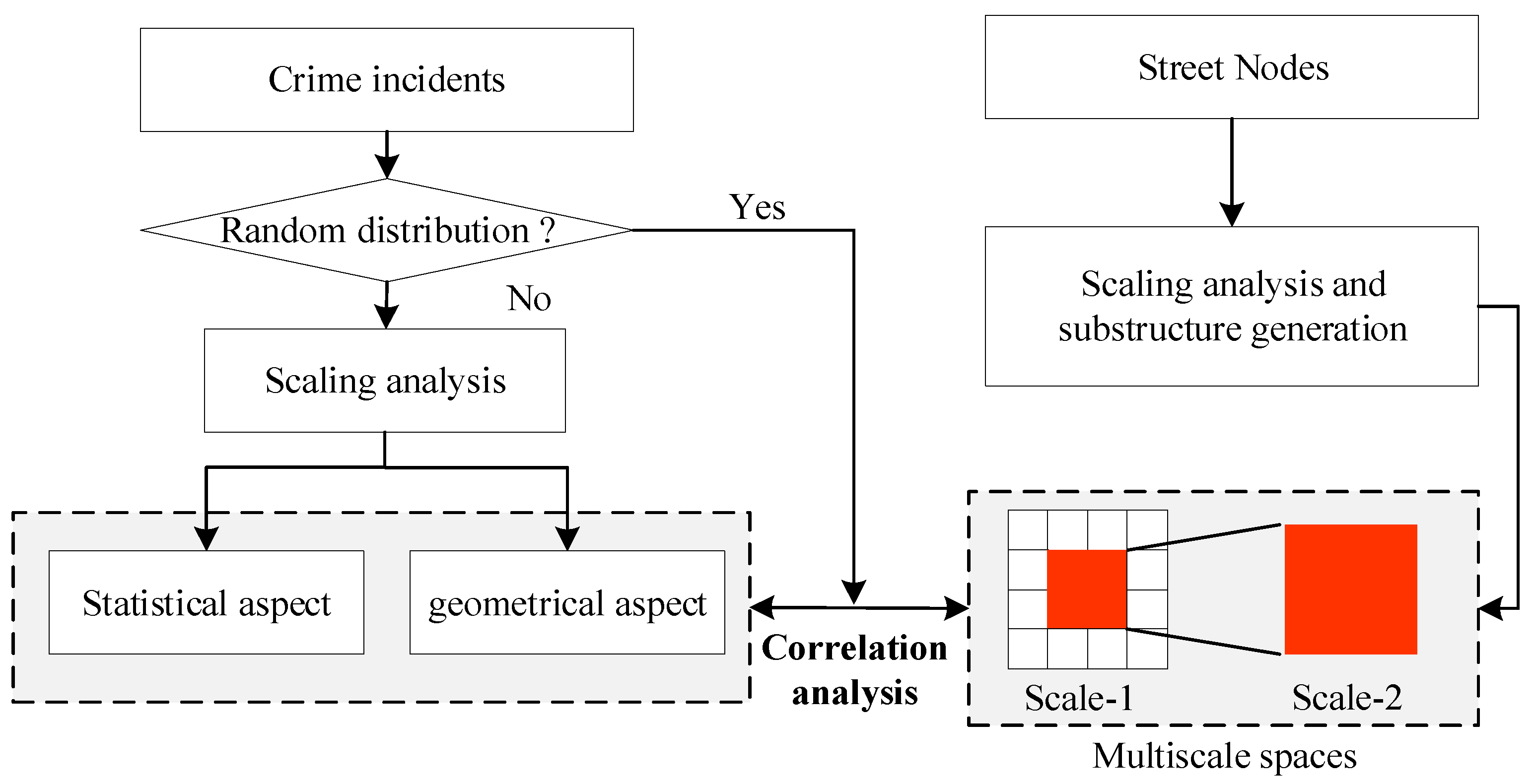
3.1. Methodology

In this study, we borrowed the recently proposed concepts of “living structure”, “natural cities” and “topological representation” in geographic information science [40,41,49]. In the domain of geographic information science, spatial data are often represented by a raster or vector data format, and geographic space is abstracted as either a large set of pixels or a variety of points, lines and polygons. Recently, some research argued that geographic space is just a collection of numerous lifeless pieces (e.g., pixels, points and lines) under conventional geographic representations, which pose little meaning in space cognition. In real geographic space, entities are connected to other things, to constitute even larger things, forming a hierarchy of recursive entities or subspaces (e.g., the street, neighborhood and city). Under such a worldview, the world is an unbroken whole that possesses a physical structure, called a “living structure”. The living structure can be represented as a hierarchy of recursive subspaces, which is a truly multiscale representation for geographic space. The concepts of natural cities refer to spatial patches adaptively portrayed by the density of spatial features (e.g., the street nodes, points of interest, etc.) and head/tail breaks [50], which are different from conventional concepts of cities defined by census authorities. The detailed process of generating natural cities can be found in Jiang’s research [51]. The living structure is closely related to natural cities, referring to the fact that the spatial centers of natural cities support each other and form an organic whole. Topological representation is the method used to describe the living structure, which aims to build up a supporting relationship for hierarchical natural cities using a complex network. The detailed description for living structure generation and topological representation can be found in related studies [40,41,51].

To achieve the research goal of this study, two kinds of geographic data were adopted, i.e., crime incidents and street nodes. The analysis of the heterogeneity of crime distribution is based on crime incidents and the underlying geographic space, which can be generated by the street nodes. Specifically, crime heterogeneity can be analyzed from two aspects. First, the aggregation of crime is checked by random distribution testing (e.g., the spatial statistic described in Section 2.1), although the distribution of crime incidents often violates the random distribution and exhibits a clustering tendency. In addition, the heterogeneity is also described by a scaling analysis method while considering both the statistical and geometrical distribution [40,41]. The key idea of scaling analysis is to describe the geographic distribution from multiple scales, specifically, by representing the geographic distribution as a hierarchy of recursive clusters or subspaces. To explore the influence of multiscale geographic space on crime, “living structure” and “natural cities” are generated by the street nodes, then geographic space can be represented as a hierarchy of recursive subspaces [41]. Finally, the correlation between crime distribution and underlying natural cities could be analyzed at multiple scales. The general research strategy of this study is shown in Figure 1.

3.1.1. Scaling Analysis for Spatial Heterogeneity

In this study, scaling analysis is used to describe the spatial heterogeneity. It consists of two aspects: scaling analysis about the statistical distribution and scaling representation about the geometric distribution.

• Scaling analysis on the statistical distribution

Scaling analysis on the statistical distribution aims to describe the skewed distribution of geographic events. Two common skewed distributions are the power law distribution [48] and the heavy-tailed distribution [50]. A simple way to detect a power law distribution is by creating a log–log plot of the data. If the data follows the power law distribution, a descending line will appear on the log–log plot. In real application, a more robust approach to judge the power law distribution is by calculating two parameters, i.e., the power law exponent α and the goodness-of-fit index p-value [52]. Formally, the power law exponent α is calculated as follows:

$$\alpha =1+n{\left[{\displaystyle \sum _{i=1}^n\ln \left(\frac{x_i}{x_{\min }}\right)}\right]}^{-1}$$

(1)

where the x_min is the smallest value in the data. The α falling in the range (1, 3) indicates a power law distribution. In addition, a goodness-of-fit index p-value is used to measure how well the data fits a power law distribution. The minimum p-value is zero and indicates the non-power law distribution, while the maximum p-value (i.e., 1) indicates a perfect power law distribution. In practice, a p-value threshold should be given to judge an acceptable power law distribution. Following the practices in previous research [18], the p-value threshold is set as 0.01.

Another way to describe the skewed distribution is based on the head/tail breaks, which divides the data values into two classes (i.e., the head part and tail part) around the mean. For a skewed distribution, the proportion of values in the head and tail would be imbalanced. The head/tail breaks partition continues iteratively until the head part values are no longer heavy-tailed. The number of head/tail partitions can also be used to measure the data skewness. Jiang et al., defined the ht-index, to measure the heterogeneity of data distribution, as the number of head/tail partitions plus one [50]. Compared with the power law distribution, the ht-index can describe a wider range of distributions (e.g., the exponential distribution). Therefore, in this study, the scaling analysis on statistical distribution is measured by three parameters: the power law exponent α, the goodness-of-fit index p-value and the ht-index value ht.

2.

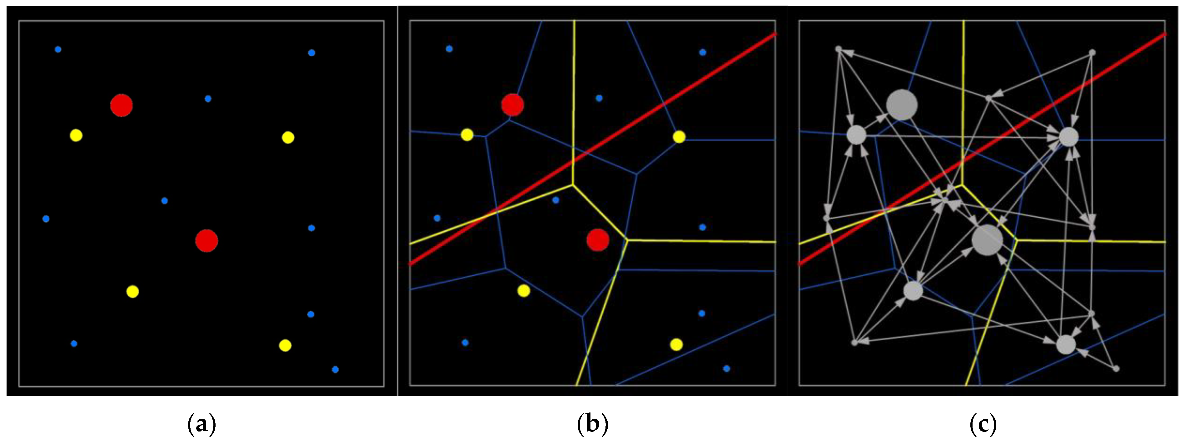
Scaling analysis on geometric distribution

The scaling analysis on geometric distribution aims to identify hierarchical geographic clusters and the topological relationship. Illustration of related concepts (“natural cities”, “living structure” and the topological representation) can be found in Figure 2. In the figure, geographic clusters (e.g., crime clusters) are firstly represented by their geometric centers and then divided into different hierarchical levels according to size or importance. Then, for each hierarchy, these geometric centers are used to generate the Thiessen polygons to partition the study region. Finally, a complex network can be constructed based on polygon–polygon relationships, i.e., small polygons point to large ones at the same level, and contained polygons point to containing polygons across two consecutive levels (as illustrated in Figure 2c). In this way, the spatial heterogeneity can be modelled by incorporating the scale property. The topological representation not only tells “where the clusters are”, but also tells “how important this center is” and “why the center is important” by revealing the hierarchy information and its topology relationship. To quantitatively measure the liveness (or importance) of nodes in the complex network, both the city sizes and Google’s PageRank (PR) scores can be used. More specifically, the sizes measure the degree of livingness in the current status, and the PR score measures the degree of livingness in the future.

3.1.2. Multiscale Association between Geographic Space and Crime Distribution

Based on the scaling analysis method, both the crime distribution and street nodes can be divided into several hierarchies based on the concept of natural cities and scaling analysis approach. Since natural cities refer to spatial patches adaptively portrayed by the density of spatial features, they have different meanings when applied to different data. For crime distribution, the derived natural cities describe the crime clusters in different hierarchies. For street nodes, natural cities describe a hierarchy of geographic subspaces with varying degrees of livingness. Based on the multiscale crime hotspots and underlying subspace, the correlation between spatial environment and crime can be analyzed. In previous research, a Pearson’s correlation coefficient was applied to analyze correlations at the different scales [40,51]. Inspired by the development of spatio-temporal data mining techniques, the clustered spatial co-location rule [53] is adopted to describe the association between spatial environment and crime distribution in this study. Given X and Y as sets of layers, a clustered spatial co-location rule is defined as follows:

$$X\Rightarrow Y\left(CS,CC\right)$$

(2)

where X and Y are termed as antecedent and consequent, separately. The CS is termed the “clustered support”, defined as the ratio of the area of the cluster (region) that satisfies both X and Y to the total area of the subspace (i.e., X). The “clustered confidence” (CC) is defined as the ratio of the area satisfying both X and Y to the total area of the cluster region of Y. From the definition, the clustered support measures the percentage of subspace overlapping with the crime clusters, while the clustered confidence indicates the percentage of crime clusters explained by the subspace. Together, the two indicators in the clustered spatial co-location rule could explain the correlation among different spatial features without normal distribution or linear relationship assumption.

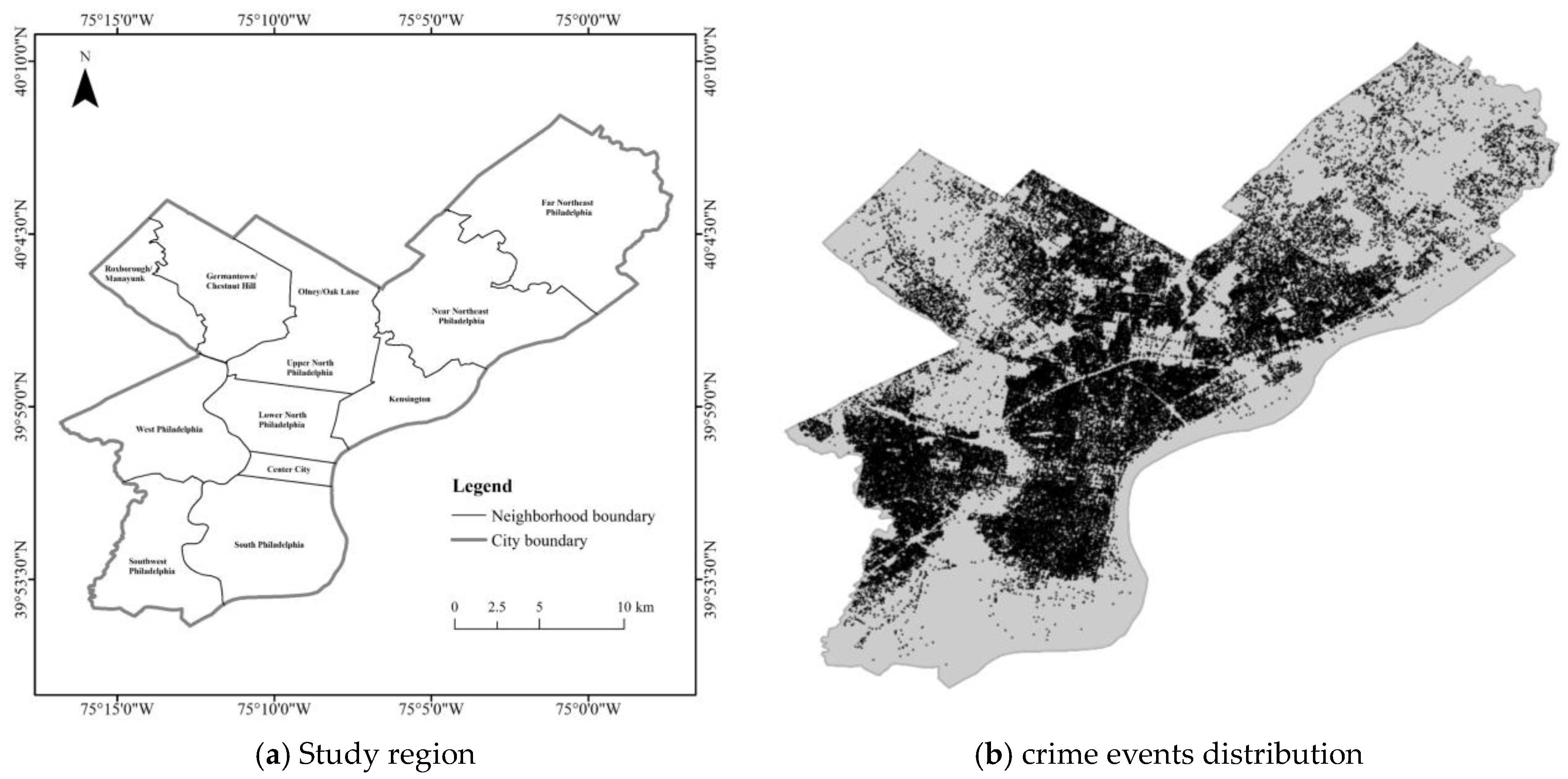
3.2. Data Description

In this study, both the crime and street node data in the city of Philadelphia are collected. Both the crime data and street nodes data can be accessed from the Philadelphia Police Department (https://www.opendataphilly.org/, accessed on 1 June 2022). Located in southeastern Pennsylvania, Philadelphia is an economic and cultural anchor of the greater Delaware Valley, with a population of 1,580,863 (based on 2017 census-estimated results). The crime occurrence in Philadelphia consistently ranks above the national average, which is a major concern for the government of the city of Philadelphia. In this study, we mainly focus on crime occurrences in the years of 2019, considering the dramatic changes (e.g., regarding the social inequality) caused by COVID-19. During this period, there are 25,427 street nodes and 159,313 crime incidents in total, which is mainly composed of violent crimes (e.g., robbery) and property crimes (e.g., theft). The distribution of the study region and crime data are shown in Figure 3. The numbers of crime incidents are so huge that it is difficult to identify specific spatial patterns. However, the distribution of crime and street nodes are highly similar by simple visual comparation.

4. Results and Discussions

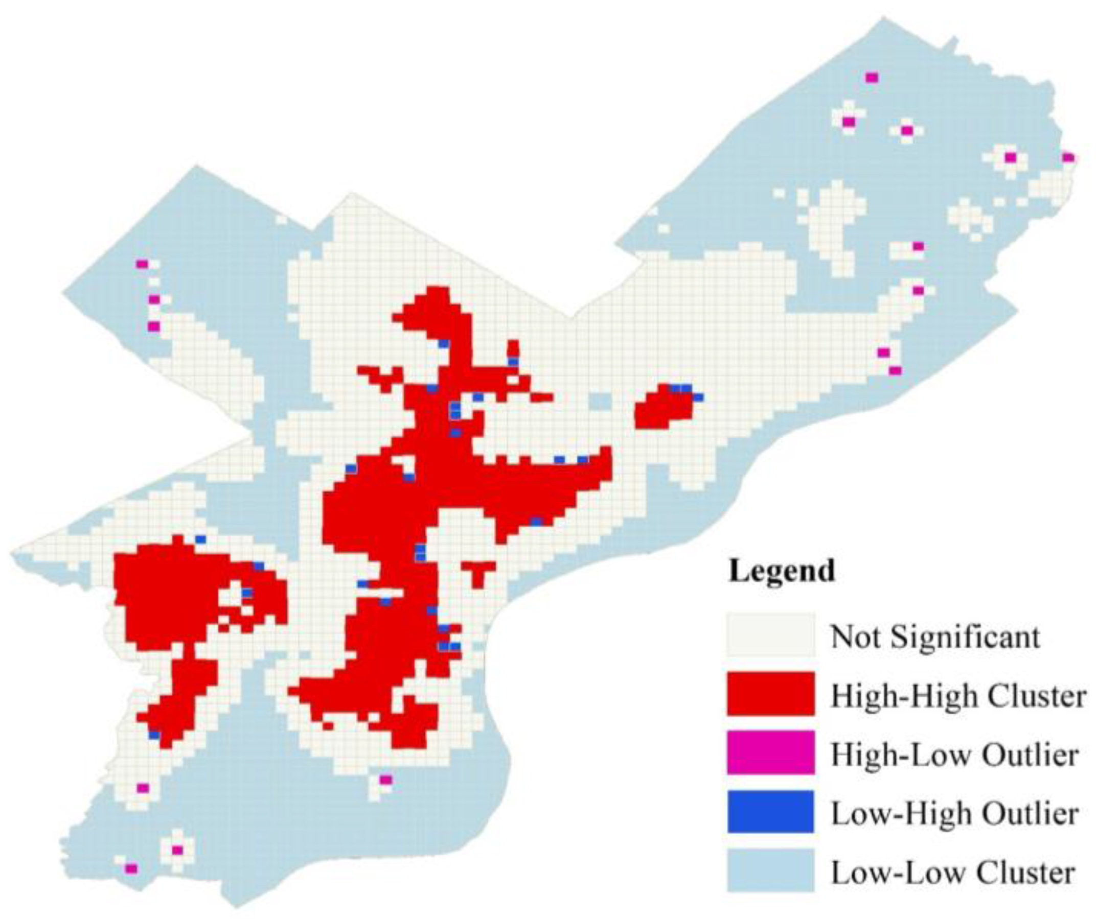
4.1. Scaling Analysis for the Heterogeneity of Crime Distribution

First, whether the crime distribution follows random distribution is tested. To do that, the crime incidents are first mapped to the spatial grid with a size of 600 × 600 m. The selection of grid size is based on experience in previous studies [17,21]. Then, Local Moran’s I is adopted to check the clustering tendency of crime incidents. The Local Moran’s I can identify both the spatial clusters and spatial outliers. It also distinguishes between a statistically significant cluster of high values (i.e., High-High cluster), cluster of low values (i.e., Low-Low cluster), outliers in which a high value is surrounded by low values (i.e., High-Low outlier), and outliers in which a low value is surrounded primarily by high values (i.e., Low-High outlier). The result of Local Moran’s I is shown in Figure 4. The results once again prove the fact that the spatial distribution of crime is not randomly distributed. The concentration of crime incidents may be related with spatial environmental factors.

To further explore the multiscale heterogeneity, the scaling analysis approach is applied. Specifically, the Delaunay triangulation network is first generated based on the crime incidents. Then, the head/tail break is applied to divide edges of the network into head and tail parts based on an edge’s length. Following the practices in previous studies [40], the head/tail proportion is set as 0.4. Finally, the edges in the tail parts (high-density regions) are transformed into polygons and then merged to generate the natural cities. In this sense, the natural cities correspond to the clusters of crime distribution and can be regarded as the crime hotspots. The operation process described above can be recursively applied and hierarchical crime hotspots can be generated. As illustrated in Figure 5, crime hotspots at different levels of scale are in a nested relationship, i.e., Level Ⅲ $\subset$ Level Ⅱ $\subset$ Level I. It can be learned that crime events are heterogeneously distributed at different scales. A deeper look into a hotspot on a larger scale (e.g., the largest hotspot in Philadelphia) will reveal that the crime distribution inside the hot spot is still heterogeneous. To quantitatively describe the multiscale heterogeneity of crime distribution, the related measuring indexes are calculated and presented in

Table 1. Measuring indexes for multiscale crime hotspots.

	Ht	#NC	#NC_head	%NC_head	MaxArea	MeanArea	#crime	%crime_head
Level Ⅰ	5	2943	114	3.87	10.556	0.021	159313	69.2
Level Ⅱ	4	711	88	12.38	0.616	0.003	19194	56.14
Level Ⅲ	3	71	12	16.9	0.034	0.002	4539	73.23

Ht: ht-index; #NC: number of natural cities; #NC_head: number of natural cities in head; %NC_head: percent of natural cities in head; MaxArea: maximum area of the natural cities (km²); MeanArea: average area of the natural cities (km²); #crime: number of crime incidents; and %crime_head: percentage of crime in head part.

and Figure 6.

In Table 1, the “natural cities” describe the clusters of crime incidents. As shown in the Table, the crime distribution in all three levels is heterogeneous, which can be reflected by the ht-index value. Usually, an ht-index above 3 will indicate the heterogeneous distribution [40]. The heterogeneity of crime distribution also can be reflected by the number of crime clusters (i.e., columns 4 and 5) and their areas (i.e., columns 6 and 7). Although the head/tail break is around the mean area of clusters, the percentage in the head part is always less than 20%. Meanwhile, the maximum area of the crime cluster is far away from the average area, which also indicates the skewness of the distribution. The last column in the table indicates that the small proportion of crime clusters covering the majority of crime incidents, which is consistent with the statement about the law of concentrations of crime at place [6].

As shown in Figure 6, the areas of crime hotspots at different scales fit the power-law distribution well, with α falling in the range (1, 3) and a p-value above 0.01. The similarity among different scales demonstrates the fractal nature of geographic phenomena; that is, the distribution of geographic phenomena appears similar in spatial pattern at various scales. As one major spatial property of geographic phenomena (e.g., crime events), spatial heterogeneity also exists across multiple scales. In previous research, however, the crime heterogeneity often is analyzed at a single scale, for example, by spatial statistics such as Local Moran’s I, which is illustrated in Figure 4. By comparing Figure 4 and Figure 5, it can be learned that the scaling analysis can describe the crime heterogeneity more accurately. Without considering the scale effect, non-hotspot regions at fine scale may be incorrectly identified as hotspot regions at coarse scale.

Finally, the scaling analysis on geometric distribution is implemented. All derived hotspots are abstracted as individual points and put into different hierarchical levels based on their sizes and the head/tail breaks. Then, these points of different hierarchical levels are used to create Thiessen polygons, and the topological representation for hierarchical hotspots is shown in Figure 7. In Figure 7, crime hotspots in different scale are represented by their geometric centers, and the hierarchy of hotspots are reflected by both the color and size of the centers. From Figure 7, it is easy to identify the location and significance of crime hotspots in each level by simply checking the size of their centers. In addition, the distribution of crime hotspots is not random, but exhibiting the property of a living structure, i.e., there are far more small centers than large ones and centers in different levels support each other to form the final complex and coherent structure. Specifically, the clusters in the high level are in fact related with and supported by a set of clusters at low levels. If the crime occurrence is influenced by the spatial environment, then the formation of the complex structure may be related with the complex underlying spatial structures.

4.2. Multiscale Association between Crime and Spatial Environment

The association analysis between crime and underlying geographic space is analyzed at multiple scales. To do that, the street nodes are further used to generate natural cities at different levels of scale, and then the multiscale natural cities are regarded as the fundamental subspace where crime events occur. The reason behind the operation is that underlying geographic space determines human mobility or human activities, and human mobility is a critical factor for crime occurrence which has been widely verified by environmental criminal theories [12,13,14]. The hierarchical subspace generated by street nodes is shown in Figure 8. By a visual comparison of Figure 5 and Figure 8, it can be found that there is a high similarity between the distribution of crime hotspots and the underlying subspaces. To quantify the correlation, we overlap the crime distribution and the generated hierarchical subspace, which is shown in Figure 9. Then, the clustered spatial co-location rule is applied to measure the spatial correlation. In this study, we mainly concern the influence of underlying geographic space on crime distribution; therefore, only two kinds of factors are considered, i.e., the underlying subspace and crime hotspots. Specifically, the clustered spatial co-location rule is simply expressed as “underlying space → crime distribution”, while treating the subspace as antecedent and crime distribution as consequent. The related indexes in the rules are in

Table 2. Correlation explained by clustered association rules.

	Subspace Area (km2)	Hotspots Area (km2)	Overlapped Area (km2)	CS	CC
Level 1	120.017	62.441	53.967	44.97%	86.43%
Level 2	15.636	11.325	4.819	30.82%	42.55%
Level 3	2.036	1.114	0.654	32.12%	58.71%

.

In the Table 2, CS is short for clustered support and CC is short for clustered confidence, which have been defined in Formulate 2 in Section 3.1.2. Specifically, the CS measures the percentage of subspace overlapping with the crime clusters and CC indicates the percentage of crime clusters explained by the subspace. For example, the first row in the Table can interpreted as “without any other auxiliary data, given the subspace described in Figure 8a, more than 86 percent of crime distribution can be explained by the subspace, and these crimes are distributed in nearly 45 percent of area in the subspace”. From the table, it can be learned that the underlying subspace described by natural cities have a good correlation with crime distribution. In Level 1, the underlying subspace can explain about 86 percent of crime hotspots. That is to say, the spatial heterogeneity of crime on a large scale (e.g., the whole city level) is mainly explained by the physical structure of spatial environment, which is represented by geographic subspaces (i.e., natural cities) in this study. These subspaces are closely related to the density of existing spatial features, for instance, the street nodes or points of interest. If we want to predict the distribution of crime at this scale, there may be no need for too much auxiliary data, for example, the street view images. In Level 2 and Level 3, the underlying subspace can explain 42.55% and 58.71% of the crime clusters. That indicates a declined association between geographic space and crime occurrence. That means, if we try to figure out the influencing factors for crime occurrence at a small scale, we may need more related data, for example, socioeconomic data or street view data. In addition, the association between geographic space and crime distribution declines in a non-liner manner when spatial scale changes, which manifests a complex mechanism between influencing factors and crime occurrence. Specifically, the influence of spatial environment on crime varies with the spatial scale of underlying geographic space.

In this study, we also compare the Pearson’s correlation coefficients at natural cities (generated by street nodes) level, following the practices in previous studies [46]. The results are listed in

Table 3. Pearson Correlation at natural cities.

	Size/Crime	Life/Crime	Street Node/Crime	%Street Node	%Crime
Level 1	0.993 **	0.937 **	0.995 **	0.87	0.74
Level 2	0.864 **	0.858 **	0.834 **	0.74	0.37
Level 3	0.930 **	0.961 **	0.905 **	0.88	0.54

**: Statistically significant at the level of 0.01.

. In the table, the ‘Size/Crime’ and ‘Life/Crime’ columns indicate the correlation between crime and size and PageRank score of natural cities. It can be learned that both the size and configuration (i.e., the support relationship) of these natural cities are positively correlated with crime distribution. The ‘Street node/Crime’ column indicates the correlation between counts of street nodes and crime incidents, and the last two columns measure the percent of street nodes and crime incidents falling in natural cities. As shown in Table 3, the correlation between street nodes and crime distribution is higher than 0.8 in all three levels. However, Pearson’s correlation coefficients only consider the statistical information in the natural cities, without considering both the data distribution (e.g., the normal or power law) and the spatial adjacent relationship (i.e., whether street nodes are collocated with crime incidents). Therefore, the Pearson’s correlation at natural cities level will, in fact, overstate the correlation between street nodes and crime distribution. Considering the spatial overlap, the correlation between crime and street nodes would decline, as shown in the last column in Table 2. Even so, subspace generated by street nodes can predict the crime hotspots well, especially at large scale (e.g., the Level 1).

4.3. Discussion

This study adopts a multiscale analysis method to quantitatively measure the heterogeneity of crime distribution. The multiscale method extends the current criminological research regarding crime pattern analysis. Most previous studies only explore crime heterogeneity from the mechanistic perspective, which treats geographic space as a collection of points or lines and then analyzes the crime distribution at single scale. In this study, inspired by a recent theory about “living structure” in geographic information science, we adopt another worldview, which represents geographic space as a hierarchy of recursive subspaces. The new representation of geographic space can pose more meaning in space cognition and crime understanding. In addition, by applying the scaling analysis on both the statistical and geometric distribution of crime, the crime heterogeneity can be fully measured. Based on the methodology in this study, we can answer questions such as “how are the crime incidents distributed at different spatial scales?” and “where are the crime clusters given a specific spatial scale?” The analysis on crime heterogeneity proves that the crime distribution is also often characterized by the 80–20 principle; that is, most of the crime incidents are distributed in a few hotspot areas. The heterogeneous distribution can be found at different spatial scales. This study also explores the multiple associations between crime hotspots and underlying geographic space (i.e., subspace generated by street nodes). The results show that the underlying subspace can explain the crime concentration well, especially at a large scale. As illustrated in Table 2, the subspace generated by street nodes can explain about 86% of the crime clusters at the city scale. In fact, it is not surprising that only the street nodes explain crime distribution to such an extent. Such results can be easily explained by existing environmental criminal theories. For example, routine activity theory believes that crimes would occur at the intersection of motivated offenders, suitable targets and the absence of capable guardians. All these factors may be related with human mobility. As the skeleton of the city, streets are closely related with urban vitality and even shape human movements, which further creates crime opportunities. However, most crimes actually occur in micro-spatial scenes, which may be influenced by surrounding facilities (e.g., crime generator or attractor), perception of the built environment (e.g., the disorder and decay) and even the natural environment condition (e.g., raining) [54]. As a result, street nodes explain crime distribution to a lesser extent on a fine scale. Establishing a more precise relationship between crime and spatial environment may depend on other types of data (e.g., the street view images).

We believe that the multiple associations between underlying geographic space and crime heterogeneity are helpful for crime analysis in practice, including crime pattern analysis, crime explanation and even crime prevention. Most previous studies mainly focus on spatial dependence at a specific scale in crime pattern analysis, while this study extends the previous work by exploring uneven distribution at multiple scales. In addition, the multiscale heterogeneity of crime also reminds practitioners that the spatial scale effect should be considered when exploring the influencing factors. Specifically speaking, the major influencing factors may be different at different spatial scales. Correspondingly, the scale effect should also be considered when making crime prevention decisions. The results in this study suggest that effective crime prevention measures should pay more attention to a small portion of data on a fine scale.

5. Conclusions

As a major characteristic of spatial data, spatial heterogeneity should never be neglected in geographic information science and related disciplines, for example, environmental criminology. Although it is widely accepted that crime incidents are usually heterogeneously distributed, most previous studies focus on the uneven distribution at a specific spatial scale. In this study, we summarize several implications of spatial heterogeneity, and point out that multiscale issues should also be considered in studying crime heterogeneity. Therefore, this study developed a multiscale analysis method to quantitatively measure the heterogeneity of crime distribution while simultaneously considering the statistical and geometrical characteristics of crime distribution. Then, inspired by the spatial data mining technique, the clustered spatial co-location rule mining approach was applied to explore a multiscale association between crime distribution and the underlying geographic space. Experimental results showed that the proposed approach can reflect the multiscale nature of crime heterogeneity well and effectively detect the hierarchical crime hotspots. The multiscale analysis on the association between crime and underlying geographic space reveals that the living structures or subspaces generated by street nodes play a key role in determining human mobility and crime distribution.

In the geographic big data era, the growth of data type and data volume provides geographic research with both opportunities and challenges. On one hand, more information and various relationships can be extracted, which is helpful to understanding the complex geographic phenomena. On the other hand, the increasing geographic data volume may make it difficult to identify dominant spatial patterns if the spatial scales are neglected. In this study, crime incidents over a full year were investigated. Without considering the multiscale effect, existing crime pattern analysis may find it difficult to precisely describe the crime heterogeneity and its influencing factors. The multiscale analysis method in this study could develop new penetrating insights on crime pattern and crime explanation analysis. However, we admit that this study still has some limitations. The main limitation lies in the limited data types. In this study, we only consider two types of data, that is, the crime incidents and street nodes. However, crime occurrence is affected by a variety of factors and there are complex interactions between environment and crime occurrence. Therefore, the underlying geographic space alone cannot fully explain crime occurrence. In future studies, more environmental factors (e.g., socioeconomics) should be added to quantitatively measure their influence on crime occurrence. In addition, more cities and even countries should be considered to prove the multiscale association between underlying geographic space and crime heterogeneity.

References

1. Liu, L. Progresses and Challenges of Crime Geography and Crime Analysis. In New Thinking in GIScience; Springer: Singapore, 2022; pp. 349–353. [Google Scholar]
2. Shu, H.; Pei, T.; Song, C.; Ma, T.; Du, Y.; Fan, Z.; Guo, S. Quantifying the spatial heterogeneity of points. Int. J. Geogr. Inf. Sci. 2019, 33, 1355–1376. [Google Scholar] [CrossRef]
3. Brantingham, P.L.; Brantingham, P.J. A theoretical model of crime hot spot generation. Stud. Crime Crime Prev. 1999, 8, 7–26. [Google Scholar]
4. Weisburd, D.; Bushway, S.; Lum, C.; Yang, S.-M. Trajectories of crime at places: A longitudinal study of street segments in the city of Seattle. Criminology 2004, 42, 283–322. [Google Scholar] [CrossRef]
5. Weisburd, D.; Morris, N.A.; Groff, E.R. Hot spots of juvenile crime: A longitudinal study of arrest incidents at street segments in Seattle, Washington. J. Quant. Criminol. 2009, 25, 443–467. [Google Scholar] [CrossRef]
6. Weisburd, D.; Amram, S. The law of concentrations of crime at place: The case of Tel Aviv-Jaffa. Police Pract. Res. 2014, 15, 101–114. [Google Scholar] [CrossRef]
7. Vilalta, C.J. How exactly does place matter in crime analysis? Place, space, and spatial heterogeneity. J. Crim. Justice Educ. 2013, 24, 290–315. [Google Scholar] [CrossRef]
8. Boivin, R. Routine activity, population(s) and crime: Spatial heterogeneity and conflicting Propositions about the neighborhood crime-population link. Appl. Geogr. 2018, 95, 79–87. [Google Scholar] [CrossRef]
9. Fotheringham, A.S.; Yang, W.; Kang, W. Multiscale geographically weighted regression (MGWR). Ann. Am. Assoc. Geogr. 2017, 107, 1247–1265. [Google Scholar] [CrossRef]
10. Brunsdon, C.; Fotheringham, S. Geographically weighted regression. J. R. Stat. Soc. Ser. D (Stat.) 1998, 47, 431–443. [Google Scholar] [CrossRef]
11. Andresen, M.A.; Malleson, N. Spatial heterogeneity in crime analysis. In Crime Modeling and Mapping Using Geospatial Technologies; Springer: Dordrecht, The Netherlands, 2013; pp. 3–23. [Google Scholar]
12. Becker, G.S. Crime and punishment: An economic approach. In The Economic Dimensions of Crime; Springer: Berlin/Heidelberg, Germany, 1968; pp. 13–68. [Google Scholar]
13. Brantingham, P.J.; Brantingham, P.L. Patterns in Crime; Macmillan: New York, NY, USA, 1984. [Google Scholar]
14. Cohen, L.E.; Felson, M. Social Change and Crime Rate Trends: A Routine Activity Approach. Am Sociol. Rev. 1979, 44, 588–608. [Google Scholar] [CrossRef]
15. Hipp, J.R.; Lee, S.; Ki, D.; Kim, J.H. Measuring the Built Environment with Google Street View and Machine Learning: Consequences for Crime on Street Segments. J. Quant. Criminol. 2021, 38, 537–565. [Google Scholar] [CrossRef]
16. He, L.; Páez, A.; Jiao, J.; An, P.; Lu, C.; Mao, W.; Long, D. Ambient population and larceny-theft: A spatial analysis using mobile phone data. ISPRS Int. J. Geo-Inf. 2020, 9, 342. [Google Scholar] [CrossRef]
17. He, Z.; Deng, M.; Xie, Z.; Wu, L.; Chen, Z.; Pei, T. Discovering the joint influence of urban facilities on crime occurrence using spatial co-location pattern mining. Cities 2020, 99, 102612. [Google Scholar] [CrossRef]
18. Ma, D.; Osaragi, T.; Oki, T. Exploring the heterogeneity of human urban movements using geo-tagged tweets. Int. J. Geogr. Inf. Sci. 2020, 34, 2475–2496. [Google Scholar] [CrossRef]
19. Zeng, M.; Mao, Y.; Wang, C. The relationship between street environment and street crime: A case study of Pudong New Area, Shanghai, China. Cities 2021, 112, 103143. [Google Scholar] [CrossRef]
20. Tobler, W.R. A computer movie simulating urban growth in the Detroit region. Econ. Geogr. 1970, 46, 234–240. [Google Scholar] [CrossRef]
21. He, Z.; Tao, L.; Xie, Z.; Xu, C. Discovering spatial interaction patterns of near repeat crime by spatial association rules mining. Sci. Rep. 2020, 10, 17262. [Google Scholar] [CrossRef]
22. Leong, K.; Sung, A. A review of spatio-temporal pattern analysis approaches on crime analysis. Int. E-J. Crim. Sci. 2015, 9, 1–33. [Google Scholar]
23. Kennedy, L.W.; Caplan, J.M.; Piza, E. Risk clusters, hotspots, and spatial intelligence: Risk terrain modeling as an algorithm for police resource allocation strategies. J. Quant. Criminol. 2011, 27, 339–362. [Google Scholar] [CrossRef]
24. Anselin, L. The Local indicators of spatial association—LISA. Geogr. Anal. 1995, 27, 93–115. [Google Scholar] [CrossRef]
25. Ord, J.K.; Getis, A. Local spatial autocorrelation statistics: Distributional issues and an application. Geogr. Anal. 1995, 27, 286–306. [Google Scholar] [CrossRef]
26. Besag, J. Discussion of Dr Ripley’s paper. J. R. Stat. Soc. Ser. B 1977, 39, 193–195. [Google Scholar]
27. Kulldorff, M. A spatial scan statistic. Commun. Stat.-Theory Methods 1997, 26, 1481–1496. [Google Scholar] [CrossRef]
28. Lotwick, H.; Silverman, B. Methods for analysing spatial processes of several types of points. J. R. Stat. Soc. Ser. B (Methodol.) 1982, 44, 406–413. [Google Scholar] [CrossRef]
29. Miethe, T.D.; Hart, T.C.; Regoeczi, W.C. The conjunctive analysis of case configurations: An exploratory method for discrete multivariate analyses of crime data. J. Quant. Criminol. 2008, 24, 227–241. [Google Scholar] [CrossRef]
30. Summers, L.; Caballero, M. Spatial conjunctive analysis of (crime) case configurations: Using Monte Carlo methods for significance testing. Appl. Geogr. 2017, 84, 55–63. [Google Scholar] [CrossRef]
31. Bernasco, W.; Block, R. Robberies in Chicago: A block-level analysis of the influence of crime generators, crime attractors, and offender anchor points. J. Res. Crime Delinq. 2011, 48, 33–57. [Google Scholar] [CrossRef]
32. Hipp, J.R.; Kim, Y.-A. Explaining the temporal and spatial dimensions of robbery: Differences across measures of the physical and social environment. J. Crim. Justice 2019, 60, 1–12. [Google Scholar] [CrossRef]
33. Song, G.; Liu, L.; Bernasco, W.; Xiao, L.; Zhou, S.; Liao, W. Testing indicators of risk populations for theft from the person across space and time: The significance of mobility and outdoor activity. Ann. Am. Assoc. Geogr. 2018, 108, 1370–1388. [Google Scholar] [CrossRef]
34. Song, G.; Bernasco, W.; Liu, L.; Xiao, L.; Zhou, S.; Liao, W. Crime feeds on legal activities: Daily mobility flows help to explain thieves’ target location choices. J. Quant. Criminol. 2019, 35, 831–854. [Google Scholar] [CrossRef]
35. Deng, M.; Yang, W.; Chen, C.; Liu, C. Exploring associations between streetscape factors and crime behaviors using Google Street View images. Front. Comput. Sci. 2022, 16, 164316. [Google Scholar] [CrossRef]
36. Connealy, N.T. Understanding the predictors of street robbery hot spots: A matched pairs analysis and systematic social observation. Crime Delinq. 2021, 67, 1319–1352. [Google Scholar] [CrossRef]
37. Zhang, F.; Fan, Z.; Kang, Y.; Hu, Y.; Ratti, C. “Perception bias”: Deciphering a mismatch between urban crime and perception of safety. Landsc. Urban Plan. 2021, 207, 104003. [Google Scholar] [CrossRef]
38. Cozens, P.; Love, T. Manipulating permeability as a process for controlling crime: Balancing security and sustainability in local contexts. Built Environ. 2009, 35, 346–365. [Google Scholar] [CrossRef]
39. Davies, T.; Johnson, S.D. Examining the relationship between road structure and burglary risk via quantitative network analysis. J. Quant. Criminol. 2015, 31, 481–507. [Google Scholar] [CrossRef]
40. Jiang, B.; Ren, Z. Geographic space as a living structure for predicting human activities using big data. Int. J. Geogr. Inf. Sci. 2019, 33, 764–779. [Google Scholar] [CrossRef]
41. Jiang, B.; de Rijke, C. Representing geographic space as a hierarchy of recursively defined subspaces for computing the degree of order. Comput. Environ. Urban Syst. 2022, 92, 101750. [Google Scholar] [CrossRef]
42. Anselin, L.; O’Loughlin, J. Geography of international conflict and cooperation: Spatial dependence and regional context in Africa. In The New Geopolitics; Taylor & Francis: Abingdon, UK, 1992; pp. 39–75. [Google Scholar]
43. Wu, J.; Li, H. Concepts of scale and scaling. In Scaling and Uncertainty Analysis in Ecology; Springer: Berlin/Heidelberg, Germany, 2006; pp. 3–15. [Google Scholar]
44. Deng, M.; He, Z.; Liu, Q.; Cai, J.; Tang, J. Multi-scale approach to mining significant spatial co-location patterns. Trans. GIS 2017, 21, 1023–1039. [Google Scholar] [CrossRef]
45. Sherman, L.W.; Gartin, P.R.; Buerger, M.E. Hot spots of predatory crime: Routine activities and the criminology of place. Criminology 1989, 27, 27–56. [Google Scholar] [CrossRef]
46. Fotheringham, A.S.; Wong, D.W. The modifiable areal unit problem in multivariate statistical analysis. Environ. Plan. A 1991, 23, 1025–1044. [Google Scholar] [CrossRef]
47. Andresen, M.A. Testing for similarity in area-based spatial patterns: A nonparametric Monte Carlo approach. Appl. Geogr. 2009, 29, 333–345. [Google Scholar] [CrossRef]
48. Newman, M.E. Power laws, Pareto distributions and Zipf’s law. Contemp. Phys. 2005, 46, 323–351. [Google Scholar] [CrossRef]
49. Jiang, B.; Miao, Y. The evolution of natural cities from the perspective of location-based social media. Prof. Geogr. 2015, 67, 295–306. [Google Scholar] [CrossRef]
50. Jiang, B. Head/tail breaks: A new classification scheme for data with a heavy-tailed distribution. Prof. Geogr. 2013, 65, 482–494. [Google Scholar] [CrossRef]
51. Jiang, B. A topological representation for taking cities as a coherent whole. In The Mathematics of Urban Morphology; Birkhäuser: Cham, Switzerland, 2019; pp. 335–352. [Google Scholar]
52. Clauset, A.; Shalizi, C.R.; Newman, M.E. Power-law distributions in empirical data. SIAM Rev. 2009, 51, 661–703. [Google Scholar] [CrossRef]
53. Huang, Y.; Zhang, P. On the relationships between clustering and spatial co-location pattern mining. In Proceedings of the 2006 18th IEEE International Conference on Tools with Artificial Intelligence (ICTAI’06), Arlington, VA, USA, 13–15 November 2006; IEEE: Piscataway, NJ, USA, 2006; pp. 513–522. [Google Scholar]
54. Zhanjun, H.; Wang, Z.; Xie, Z.; Wu, L.; Chen, Z. Multiscale analysis of the influence of street built environment on crime occurrence using street-view images. Comput. Environ. Urban Syst. 2022, 97, 101865. [Google Scholar]
Figure 1. Research strategy of this study.
Ijgi 12 00437 g001
Figure 2. Illustration of the topological representation. (a) 15 points are categorized in three hierarchical levels, indicated by different colors, i.e., red, yellow and blue for first to third levels; (b) points in same hierarchical level are used to partition the space by generating Thiessen polygons; and the boundaries of Thiessen polygon partitions are represented by lines in corresponding color; (c) topological representation, i.e., a complex network is constructed based on polygon–polygon relationships, and links in the network are represented by gray lines with arrows.
Ijgi 12 00437 g002
Figure 3. Study region and crime events distribution.
Ijgi 12 00437 g003
Figure 4. Spatial clusters of crime distribution detected by Local Moran’s I.
Ijgi 12 00437 g004
Figure 5. Spatial distribution of natural city for crime distribution. (a) Level Ⅰ: Philadelphia and its natural cities (the largest natural city is termed Level Ⅱ), (b) natural cities at Level Ⅱ (the largest one is termed Level Ⅲ), and (c) natural cities at Level Ⅲ.
Ijgi 12 00437 g005
Figure 6. Scaling analysis on statistical distribution for multiscale crime hotspots: (a) crime_level1; (b) crime_level2; and (c) crime_level3.
Ijgi 12 00437 g006
Figure 7. Scaling analysis on geometry distribution. (a) the hierarchy of levels and Thiessen polygon partitions for crime hotspots (represented by their geometric centers) at level 1; (b) the hierarchy of levels and Thiessen polygon partitions for crime hotspots at level 2; and (c) the hierarchy of levels and Thiessen polygon partitions for crime hotspots at level 3.
Ijgi 12 00437 g007
Figure 8. Multiscale subspace generated by street nodes. (a) the subspaces at level 1; (b) the subspaces at level 2; (a) the subspaces at level 3.
Ijgi 12 00437 g008
Figure 9. Overlay analysis of distribution of crime hotspot and underlying subspaces. (a) the overlay of crime hotspots and subspaces at level 1; (b) the overlay of crime hotspots and subspaces at level 2; (c) the overlay of crime hotspots and subspaces at level 3.
Ijgi 12 00437 g009