Abstract
Climate change and overpopulation have led to an increase in water demands worldwide. As a result, land subsidence due to groundwater extraction and water level decline is causing damage to communities in arid and semiarid regions. The agricultural plain of Samalghan in Iran has recently experienced wide areas of land subsidence, which is hypothesized to be caused by groundwater overexploitation. This hypothesis was assessed by estimating the amount of subsidence that occurred in the Samalghan plain using DInSAR based on an analysis of 25 Sentinel-1 descending SAR images over 6 years. To assess the influence of water level changes on this phenomenon, groundwater level maps were produced, and their relationship with land subsidence was evaluated. Results showed that one major cause of the subsidence in the Samalghan plain was groundwater overexploitation, with the highest average land subsidence occurring in 2019 (34 cm) and the lowest in 2015 and 2018 (18 cm). Twelve Sentinel-1 ascending images were used for relative validation of the DInSAR processing. The correlation value varied from 0.69 to 0.89 (an acceptable range). Finally, the aquifer behavior was studied, and changes in cultivation patterns and optimal utilization of groundwater resources were suggested as practical strategies to control the current situation.
1. Introduction
Groundwater aquifers are one of the most valuable water resources in many parts of the world [1]. Climate change and rapid population growth, however, are putting groundwater aquifers under pressure, particularly in densely populated areas in arid and semiarid environments [2]. Hence, frequent monitoring of groundwater level is essential to identify areas experiencing rapid depletion in groundwater resources and to move toward sustainable water management of aquifers, especially in arid areas prone to drought [3]. Land subsidence resulting from overexploitation of groundwater resources has been reported in many different parts of the world [4]. The immediate factor driving force the subsidence is considered to be the dropping of groundwater level; however, the primary factor behind this phenomenon is the existence of unconsolidated sediment deposits in the local aquifer system [5].
This phenomenon has affected many cities and regions in the world and caused serious damage to infrastructures and buildings. For instance, Beijing, the capital city of China, has suffered from land subsidence due to groundwater extraction since the 1950s [6]. The subsidence rate in this city is more than 100 mm/year [7]. Subsidence has also occurred in Mexico City in Mexico [8], California [9], Hue in Vietnam [10], Gorgan in Iran [11], Semarang in Indonesia [12], Mashhad in Iran [13], and many other cities in the world [4]. Dry climatic conditions in most inland areas of Iran have increased the dependency on groundwater resources to meet different demands [14]. More than 600 plains in Iran have confronted land subsidence due to excessive groundwater withdrawal [15]. In addition, there have been some plains identified with subsidence of 1 mm per day, indicating a critical situation [13].
A gradual or sudden settlement of the ground surface without any limitation on speed or occurrence area is called subsidence [16]. Different processes such as fluid extraction and mining result in the deformation or movement of soil materials, leading to land subsidence [17]. Excessive groundwater extraction leads to a continuous decline in groundwater level, reduces pore pressure [18], and results in compression and consolidation of the soil layer and gradual settling of the ground surface [19].
Land subsidence may result from elastic or inelastic deformation [20,21], and is in proportion to changes in the groundwater table and the compatible layer thickness [22]. For an elastic deformation in aquifers with semipermeable layers, the groundwater head must remain above the previous lowest level (stress before consolidation). If the groundwater table falls below the previous lowest level, inelastic compaction leads to permanent shifts in the solid grains, and porosity in the groundwater system will reduce [20]. Regions with massive pumping of groundwater usually experience inelastic deformation [21]. By introducing control strategies for groundwater pumping to limit its detrimental effects, a low uplift value is often observed [23,24,25]. However, only a small part of the initial compaction is recoverable when water is recharged into the aquifer [21].
To implement a proper analysis of the causing factor(s) of land subsidence in a particular site, a vital step is to obtain accurate measurements of the actual amount of subsidence that occurred at multiple points in time. At present, various methods can be used to measure the subsidence amplitude, including precise differential leveling [26] and permanent stations of the Global Positioning System (GPS), Light Detection and Ranging (LiDAR) [27], and Interferometric Synthetic Aperture Radar (InSAR) [28].
One of the most accurate and economic techniques based on remote sensing is radar interferometry. This technique evaluates the amount and range of subsidence over the whole area under study (rather than at a small number of sample points) and provides the possibility of repeated monitoring of the area relatively frequently (i.e., whenever new satellite images of the site are acquired) [29,30]. Differential Interferometric Synthetic Aperture Radar (DInSAR) is an efficient radar interferometry approach [31] that can be used to accurately detect ground movements and land deformation patterns at a high spatial resolution (~5 × 20 m in the case of the Sentinel-1) over large geographic areas [7]. DInSAR analysis can achieve up to millimeter accuracy, making it a very capable tool for land subsidence and uplift measurement under suitable conditions [32], such as short temporal and perpendicular baseline, and suitable atmospheric conditions [33]. This technique’s ability to determine land deformations from millimeters to centimeters in size makes it a suitable method for monitoring slow-moving deformation [34].
Increasing water demands and urbanization has caused overexploitation and depletion in many aquifers. Mexico, for example, includes a number of aquifers suffering from depletion, and as a result, land subsidence combined with ground fracturing. Synthetic aperture radar proved its ability to monitor land subsidence in this area for a long-term period. Maximum settlement rates in this area were recognized as 14 cm/year in 1996 and 10 cm/year in 2010–2012, and these increased to 12 cm/year from 2015 to 2020 [35] Excessive groundwater withdrawal has led to land subsidence and sinkholes in Central Anatolia in Turkey. Interferometric Synthetic Aperture Radar was used to monitor and better understand the relation between groundwater extractions and land subsidence in this area. The investigations revealed subsidence of 70 mm/year in this area, which follows the overall groundwater level changes with over 80% cross-correlation consistency [36]. The Tuscany region has been affected by land subsidence due to water overexploitation, geothermal activity, and urbanization. This area was studied using SqueeSAR processing of Sentinel-1 between 2014 and 2018. The descending images time series showed a maximum value of 55 mm/year subsidence in the Montemurlo area [37]. Sui et al. [30] studied subsidence in the Loess Plateau of China using DInSAR due to underground extraction using ALOS PALSAR data in 2007. They monitored subsidence with maximum values of 20 cm in some areas. They proposed an approach to combine InSAR results with the support vector machine regression algorithm to predict subsidence with a high level of accuracy.
The Samalghan plain, located in the North Khorasan province of Iran, is one of the most important agricultural plains in this country. It currently suffers, however, from subsidence, causing irreversible damage to the plain. Groundwater conditions in the mentioned area have become essential to be monitored and managed, as groundwater overexploitation may be a causing factor. A prior study [38] found that subsidence in the plain could be divided into two regions: a high-risk region in the west and northwest of the plain, and a low-risk region in the eastern parts. During the past decades, surface fractures have been created in the northwest Samalghan plain that is being developed. Consequently, studying subsidence in this plain is of great importance. In the previous studies conducted on Samalghan plain, subsidence was not measured over the entire plain area, and the relationship between subsidence rates and the rate of groundwater decline was not investigated. We aimed to fill these research gaps in the present study by detecting land subsidence using the DInSAR method and quantitatively analyzing its relationship with groundwater depletion. Then, the aquifer response to water recharge and discharge in terms of changes in groundwater head and land subsidence was evaluated.
2. Materials and Methods
2.1. Study Area
The study area is an important agricultural plain located in the western part of North Khorasan Province, Iran, covering an area of over 1100 km2 with an arid/semiarid climate. The location and extent of this area, simplified geology, and the piezometric well locations are presented as follows (Figure 1). This plain is located in the Kopeh Dagh geological zone, and its geographical location is limited within 37°21′–37°39′ N in latitude and 56°25′ to 57°06′ E in longitude. The high demand for fresh water in this area relies mostly on groundwater, which has increased due to growing agricultural consumption [39].
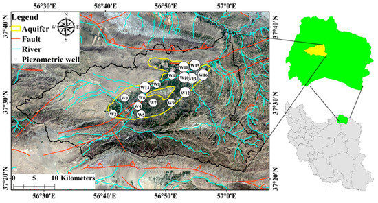
Figure 1.
Location map of study area in North Khorasan Province of Iran.
The maximum elevation is in Korkhod Mountains, 2680 m above sea level, and the minimum elevation, at the outlet of Darband, is 600 m above sea level. The average annual precipitation of this basin is approximately 465 mm, with a mean annual temperature and evapotranspiration of 11.1 °C and 1132 mm/year, respectively [40].
Based on figures obtained from the regional water authority organization of North Khorasan Province (NKHRW), this plain has 333 operational wells, with a discharge rate of 37.65 million cubic meters (MCM) per year. The number of wells experiencing overextraction in this area is 86, and the total volume of this overextraction is 17.17 MCM. An additional 1.2 MCM is extracted annually from 15 aqueducts in this plain. The aquifer recharge capacity of this plain—the maximum volume of water that can be recharged after discharge each year—is about 5 MCM/year; the current amount of extraction has caused a lack of balance in the aquifer. In terms of water quality, this plain is categorized as suitable for agricultural use and acceptable for drinking.
According to data from NKHRW, 35 MCM of the annual groundwater consumption is appertained by agriculture. The allocation of groundwater resources is represented in Figure 2. The main farmed crops in this area are cotton, rice, wheat, and barley. The density of farmlands is higher in the low-lying parts of the plain [39].
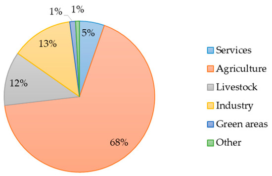
Figure 2.
Percentage of different groundwater consumption sectors in Samalghan plain.
A prior study claimed that there have been fractures reported in the northwest parts of the plain in a north–south direction. These fractures continue along a line several hundred meters in length dictated by a fault in the rock. Most of these cracks were formed in the agricultural lands and caused substantial damage to farmlands due to extra water escape and leakage into them, as well as the change of slope. As a result, farmers are constantly flattening the land and trying to eliminate the effects of cracks in agricultural lands [38].
Groundwater quality deterioration is another negative impact of these cracks. The formation of cracks can be a channel for the transfer of surface pollutants, including effluent and drainage from the agricultural lands following the use of chemical fertilizers and pesticides to the aquifer [41].
The underground geological investigations of the Samalghan plain show the variable thickness of the alluvium of this plain. In the northern part of this plain, the Tirgan formation can be observed in both the surface and the depth. The groundwater level is low in this area; therefore, most of the exploitation wells are located in this part. In the eastern part of the plain, Neogene sediments are located on the Tirgan formation, and the main lithology of these sediments is conglomerate, marl, and evaporite rocks.
The underground geological layers investigated using the log information of the existing wells in the region in three directions is shown in Figure 3a. Examining the well logs in the direction of AA’ shows that the sediments in the northeast of the aquifer are fine-grained, and the sediments change to coarse-grained towards the southwest of the area. In this regard, the thickness of the alluvium is so high that it did not meet the bedrock in the SW15 well, with a depth of 140 m. The SW2 well has encountered limestone due to its proximity to the Tirgan limestone formation. This means that along the AA’ direction, the bedrock has a great depth, and in some places it is formed of limestone.
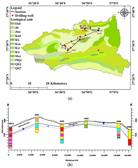
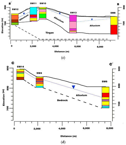
Figure 3.
The location of drilling wells for the investigation of well logs (a); (b) the log of wells in AA’; (c) the log of wells in BB’ direction; and (d) the log of wells in CC’ section.
Excavation of the drilling wells in the direction of BB’ indicates that the sediments become mostly coarse, and as the thickness of the fine-grained sediments decreases, the thickness of the coarse-grained sediments increases from east to west. In the western part of the Tirgan plain, limestone can be seen on the ground; it can also be seen in the deep parts of the northwest of the plain.
Surveys in the direction of CC’ reveal that the topographical changes decrease from the south to the north of the plain. There is a height difference of 94 m between the two wells; the water depth increases from the south to the north of the plain. Investigations in this direction indicate that the thickness of coarse-grained sediments increase from the south to the north of the plain [42].
2.2. Dataset
To study land subsidence in this plain, two series of datasets have been used: groundwater time-series data and SAR remote sensing imagery. In this section, these two datasets will be introduced.
2.2.1. Groundwater Data
To prepare and study the groundwater level change maps, piezometric data of the studying area are needed. In this study, the piezometric data consist of monthly groundwater level time series at 16 well sites covering the period of 2008–2018, provided by the Iran Water Resources Management Company (http://wrs.wrm.ir/ (accessed on 27 December 2019)). First, the historical groundwater level data were collected and sorted by year, then the trend changes in water level over each well, and also the average changes in water level in the area were studied. The groundwater level for 2019 and 2020 was predicted with the use of historical data and the best-fitted trend line in Excel. Therefore, various trendlines were fitted in this process, and the most accurate estimation was implemented according to the available data. To carry this out, exponential, linear, logarithmic, polymonal with power 2, and power trendlines were evaluated using cross-validation. The well locations can be seen as presented in Figure 1. In this study, the IDW (inverse distance weighted) method with a power value of 1, 2, 3, and 4, and ordinary Kriging and Spline methods were conducted for interpolation of groundwater levels, and their performances were evaluated by cross-validation. Then, the most accurate method was chosen as the interpolation method to develop wall-to-wall groundwater level maps of the study site.
2.2.2. SAR Data
Utilizing the radar interferometry method, the rate and trend of subsidence in Samalghan plain were investigated using the Single Look Complex (SLC) radar data stacks of the Sentinel-1 Satellite. In this study, Sentinel-1A data provided in the Copernicus database Sentinel-1 SAR, which is freely available through https://asf.alaska.edu/ (accessed on 22 January 2021), were used. The 12-day repeat orbit cycle is expected to increase the coherence value of interferometric pairs for land deformation monitoring. The Sentinel-1 data were acquired in interferometric wide (IW) swath mode, which is made up of three subswathes (IW1, IW2, and IW3) with a total swath of 250 km [8]. This mode enables coverage of a large area with a good spatial resolution [43] of 5 × 20 m for SLC-type data [44].
A total of 24 pairs of images in VV polarization were processed with the use of the conventional DInSAR technique. Appropriate selection of the data pair is a vital step because the results are highly dependent on coherence values [34]. In order to increase the coherence value and reduce the speckle noise in the interferograms and enhance the results, images with the least perpendicular baseline and the temporal baseline difference between acquisition dates were selected. The data are used in a way that every 4 interferograms contain 4 seasons for each year, with the optimal perpendicular baseline value. The interferometric pairs were chosen as given in Table 1.

Table 1.
Analyzed descending datasets information, including interferogram ID (Int ID), master date, slave date, temporal baseline (days), and perpendicular baseline (meters).
The 30 m Shuttle Radar Topography Mission (SRTM) digital elevation model was used for co-registration of the data stack. Due to the nonexistence of either previous land subsidence measurement data in the study area, GPS measurement data, or precise leveling data, the displacement results could not be validated; however, the results could be deemed to be acceptable, since DInSAR is known as an acceptable methodology giving accurate results for deformation in most areas [5]. Therefore, 11 pairs of ascending-direction images from 2018 to 2020, which were available with the optimum baseline value in the same path, were used for the validation of DInSAR the process.
2.2.3. Additional Data
In order to investigate the hypothesis that groundwater has an impact on land subsidence in the Samalghan plain, the impact of other factors such as railways and earthquakes was also examined. In order to investigate the effect of tectonic conditions and continuous earthquakes on subsidence in the region, earthquakes with a magnitude of 4 [45] or above on the Richter scale were prepared from the Seismological Center of the Institute of Geophysics, University of Tehran. In the period under study, there is no earthquake above magnitude of 4 with its center in Samalghan plain or a short distance from the region. These earthquakes do not have much effect (in centimeters) on the displacement of the study area. In addition, there is no rail line in the study area, so the impact of these two cases was ignored.
Soil type data were not available in the area, so geological information from the area was used. The information obtained from a previous study [42]. Finally, according to the study of geological maps in the study area, the relationship between subsidence loss and soil granulation was studied.
2.3. DInSAR Method
As mentioned earlier, the method employed to monitor subsidence in the Samalghan plain was DInSAR, due to its high accuracy and speed of monitoring. With the usage of this technique, accuracy in millimeters or centimeters is achievable for the velocity of land deformation [46].
The DInSAR process is conducted using the SNAP software developed by the European Space Agency (ESA) (https://step.esa.int/main/toolboxes/snap/ (accessed on 31 March 2020)). The conventional DInSAR process is shown in Figure 4 for a single-pair DInSAR. To reduce the decorrelation in interferograms and its relevant errors, the master acquisition was chosen based on the measured temporal and spatial baselines to achieve an appropriate coherence in interferograms [47]. For the descending data, the image taken later (after the event, e.g., 2020) was used as the master. In order to perform interferometric processing, two or more images were coregistered as a stack [48,49]. This step causes each ground target in both images to be identified in the same position [50]. At this point, to correct azimuth and amplitude estimations, enhanced spectral diversity (ESD) [51] was used.
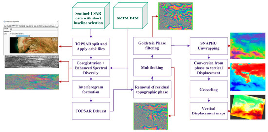
Figure 4.
Conventional DInSAR workflow in SNAP.
An interferogram contains information about both topographic and surface movement. In other words, the interferometric phase is a measure of the difference in the path length between the target and the two sensor positions [28,52]. The DInSAR technique aims to separate the contribution of the topographic phase of the earth’s surface and the portion of the displacement phase to show the extent of the displacement. In order to remove the topographic phase effect, an additional interferogram or a digital elevation model is required [53]. The 30 m SRTM Dem was used to remove the flat earth effect [54,55] and phase pixels due to the topography.
The interferograms were then filtered by Goldstein phase filtering [56] in order to remove the noise from radar instruments and temporal decorrelation [5]. Subsequently, they were unwrapped using the minimum cost flow (MCF) algorithm with SNAPHU [57,58]. Then, the unwrapped interferograms were converted into line-of-sight (LOS) displacement maps.
The vertical displacement map of the earth was prepared and geocoded. After developing Samalghan land subsidence maps, a cumulative displacement map, which is the sum of all displacements of all segments, was produced for each year. Next, the maps were examined, and the relationship between land subsidence and groundwater changes in the study area was investigated.
3. Results and Discussion
To investigate the interaction behavior of the aquifer and to evaluate the land subsidence in the Samalghan plain, radar images were processed. Secondly, the piezometric well data in the area were used to investigate groundwater level changes, then the relation between groundwater level changes and land subsidence was studied. This section will discuss the findings of the research.
3.1. Groundwater Level Variation
The trend in average annual groundwater level in the study period was plotted, and the best trend line was fitted, as shown in Figure 5. From this, it can be seen that the average depth of groundwater increased from 2008 to 2018 (i.e., groundwater level decreased). Thus, the recharge rate is significantly less than the rate of groundwater extraction. Exponential, linear, logarithmic, polymonal with power 2, and power trendlines were evaluated. The results showed that the best fitted trend line is the polymonal trendline, with a root-mean-square error (RMSE) of 0.4 (m) and correlation coefficient (CC) of 0.95 (Table 2). Using the fitted diagram trendline, the average groundwater level in 2019 and 2020 was estimated to be 24.1 and 24.9 m, respectively.
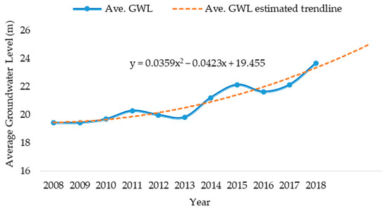
Figure 5.
Variations in average groundwater level in Samalghan plain.
Table 2.
The CC and RMSE value of the selected trendlines to estimate groundwater level.
Of the different interpolation methods and weighting parameters tested (Table 3), the ordinary Kriging method showed the lowest RMSE (1.6 m). This result is similar to that of other studies’ findings that Kriging tends to outperform IDW methods [59].
Table 3.
The RMSE value of the interpolation methods to generate the groundwater level maps.
Thus, using the observed well data, wall-to-wall groundwater level maps of the plain were generated using the ordinary Kriging interpolation method in low-height parts of the area (less than 1100 m). By overlaying the 2008 and 2018 groundwater level maps and calculating the difference (Figure 6), it is clear that the northern area saw the most significant groundwater level drop, being up to 20 m in some areas. In general, the whole plain was found to have been affected by groundwater fall. It is worthwhile to mention the fact that there are uncertainties in some parts of the region due to the lack of data and the absence of observational wells (e.g., north-west and south-east of the plain). Nevertheless, some external data (i.e., piezometric wells in a northern adjacent plain) were used to increase the accuracy in these areas.
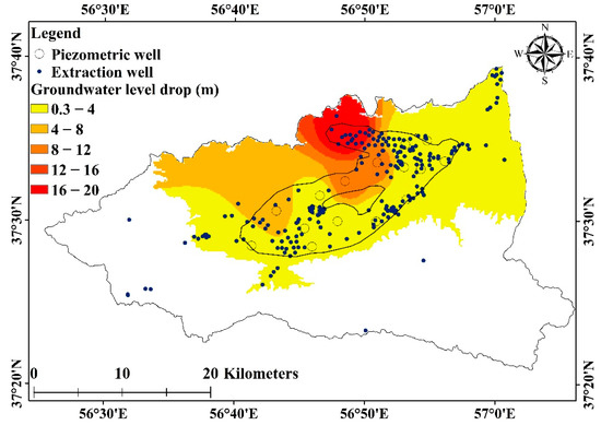
Figure 6.
Groundwater level change map between 2008 and 2018.
3.2. Displacement Maps
The results of DInSAR processing and investigation of the annual displacement maps show the pattern of subsidence over time in the study area (Figure 7). In a previous study [38], the authors pointed out that cracks have been created in the northwest of the plain, moving towards the east of the region. It can be seen that land subsidence in the Samalghan plain mainly occurred in the northern and northwestern parts of the region.
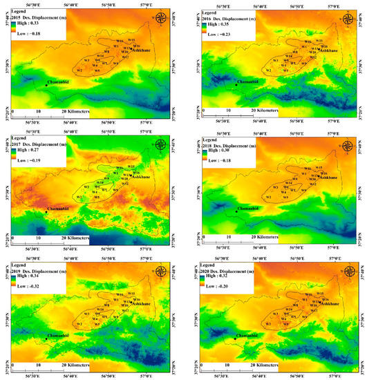
Figure 7.
Cumulative annual vertical displacement maps for 2015–2020 using descending data.
Based on deformation maps in the region, the land subsidence occurred in 2015 in all northern parts of the Samalghan plain. There was no subsidence in the south and southwest of the area in 2015. This pattern also took place in 2016. Moreover, by 2016, the maximum subsidence had reached a new peak compared to the previous year. In 2017, the land subsidence pattern changed slightly and spread to almost the entire plain. In the north of the city of Ashkhane, a slight uplift spread lightly towards the northeast–southwest of the plain. In 2018, a subsidence pattern similar to the pattern in 2015 and 2016 was detected in the Samalghan plain, which happened in all northern parts of Samalghan plain, and the pattern continues towards the central parts of the plain. Examination of the displacement maps shows the recurrence of subsidence in the north and northwest of Samalghan plain, the central part containing an aquifer, and the western part near Chamanbid in recent years. The subsidence in western parts is developing towards the Chamanbid, and if not properly managed will cause damage to residential areas. The results of field research in the city of Ashkhane and the surrounding areas showed a lot of damage to these areas, including cracks in the walls, well casing protruding, and holes in the ground.
The uplift observed in mountains is sought to have various reasons. According to information from organizations, major activities had been performed in highly elevated areas in this region. Firstly, afforestation is being conducted on an annual scale of around 70 hectares. A part of the vegetation growth can be misrecognized by uplift, as an error. Moreover, there are many villages located in mountainous areas, expanding their farmlands and plowing the bare lands, and transforming them into rainfed cultivation areas. The agricultural and urban activities in these villages are detected as uplift as well.
Following the trend of land surface changes during the study period, it is possible to observe the uplift of the ground surface after its subsidence in some places. For instance, around Chamanbid, Ashkhane, some parts of the southern part of the plain, and even the northern part of the plain in 2016, the ground surface recovered after its previous subsidence. In addition, in some areas that had been involved in subsidence in 2017, including south of the Samalghan aquifer, west and north of the Samalghan plain, and south-east of the plain, an uplift was observed in the following years. As a result, the possibility of the elastic ground behavior is high, which needs further investigation. In Figure 8, the land subsidence in the two major cities in the study area has been shown. As can be seen from the provided figure, in the city of Ashkhane, after two consecutive years of subsidence, in 2017 and 2018, an uplift was observed, and after that, two years of subsidence occurred again; however, the effect of subsidence was greater, and overall, a cumulative subsidence of 39 cm occurred at this point. In Chamanbid, the situation was different: from 2015 to 2018, an uplift was detected, while in 2019 and 2020, the trend changed and subsidence occurred.
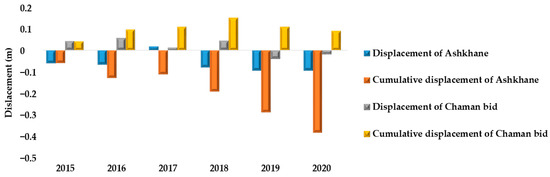
Figure 8.
The trend of annual and cumulative land deformation in Ashkhane and Chamanbid cities.
3.3. Validation
Since neither precise leveling nor GPS station data were available during the study period over the area, it is not possible to evaluate the results of InSAR processing using Earth observations. Moreover, there were no other sufficient SAR data available for the plain. Hence, a comparative validation method was used to validate the processing results in this region. For this purpose, the InSAR processing was performed using data with a different path and direction. The results were deemed acceptable if the interferometric processing results of ascending and descending satellite images of one sensor were similar [60]. The subsidence values at the piezometric well locations were also extracted in the ascending and descending displacement maps for comparison. The results showed a satisfactory result quantitatively, with a correlation of 0.69–0.89 between the subsidence estimates given by the ascending/descending data (Table 4), and a similar visual pattern in the Figure 9 maps. The slight differences between the datasets may be partially explained by the time differences between the image acquisitions.
Table 4.
Correlation of monitored subsidence for ascending and descending data at the position of piezometric wells in Samalghan plain.
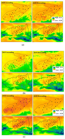
Figure 9.
Annual cumulative displacement maps for the ascending and descending data in (a) 2020, (b) 2019, and (c) 2018.
Furthermore, to determine the validity of the research findings and also to collect field evidence of subsidence in the Samalghan plain, a field operation was conducted. Subsidence has had various effects on plain areas (Figure 10). From this, we found that the effects of subsidence can be seen in the form of cracks in the ground, cracks in the walls, well casing protruding, and holes in the ground. The subsidence in some parts of the plain is accompanied by surface cracks, but in other places, it is observed as a uniform and homogeneous subsidence.
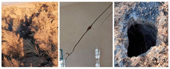
Figure 10.
Evidence of land subsidence in the study area as cracks and holes (Photographs were taken at Ashkhane on 25 February, 2021 by Rafiei, F.).
3.4. Groundwater Related Subsidence
Since this paper aimed to study the whole plain, we decided to investigate the groundwater level drop over the whole area, and although there are piezometric wells in the aquifer, there are some extraction wells outside of the aquifer (Figure 6). In addition, as can be seen, there is land subsidence in the north of the plain, even in the areas without piezometric data, but the groundwater level maps indicate that a groundwater level drop is happening there. However, to increase the accuracy, we investigated the relationship between the groundwater drop and subsidence in well locations in more detail.
To investigate the relation between water level decline and land subsidence, water level variations in the piezometric wells were overlaid with the cumulative displacement map. As shown in Figure 11, subsidence occurred in all points experiencing water level falls. In addition, in the areas where the water decline was lower, the subsidence radius value was smaller around the well. Conversely, the subsidence around the wells with a higher water level drop was spread with a greater radius. The subsidence has entirely affected the low-height parts of Samalghan, which contain a high concentration of agricultural lands and experience noticeable water extraction.
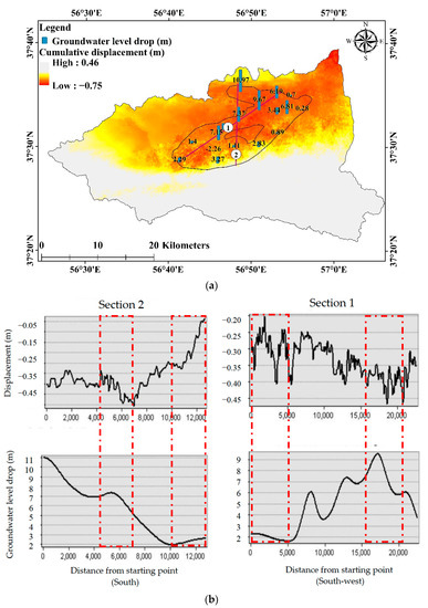
Figure 11.
(a) Change in water level and position of the piezometric wells overlaid with subsidence in the region from 2015 to 2020, with purple lines as section. (b) Sections in the aquifer showing the groundwater level drop and displacement plots.
To better understand the relationship between water level changes and land subsidence, two sections (profiles) were considered in the Samalghan aquifer. Their locations are indicated by the two lines shown in Figure 11a. The first line was drawn to cover a longer length of the aquifer in the plain and passes through the position of more piezometers. The graphs of land surface change and water level decline were then plotted in Figure 11b. It can be seen that the higher the drop in water level, the more subsidence occurs in the area. A few examples of extents with a stronger connection between water level drop and land subsidence are shown in Figure 11, indicated with the red boxes. With the lower water level fall, the rate of subsidence also decreased.
In the next step, the temporal evolution of groundwater changes and land deformation at piezometric wells are drawn on a dual-axis chart. According to Figure 12, at some wells, both changes follow almost a similar trend (Figure 12a,b), and with subsidence of groundwater, subsidence is observed. Similarly, with the recovery of the water level in the wells, an uplift is detected. However, in some wells, the ground surface with a one-year lag showed similar behavior to the water surface, as shown in Figure 12b,c.
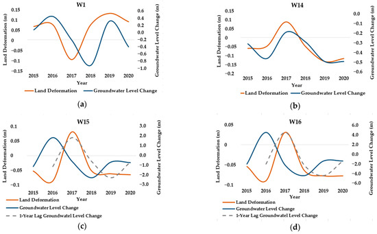
Figure 12.
Temporal evolution of deformation (InSAR estimations) (orange line), groundwater level change (blue line) at (a) well 1, (b) well 14, (c) well 15, and (d) well 16, and the groundwater level change with a one-year lag in (b,c) (gray-dashed line).
3.5. Aquifer Behavior
The following section discusses subsidence in piezometric wells in the plain, considering changes in subsidence over time.
One procedure for monitoring the relationship between the groundwater level variations and land surface changes is to plot these two parameters (groundwater level and land deformation). The authors of [61] claimed that a method can be used to estimate the approximate value of the storage coefficient of an aquifer. Based on this technique, the y-axis indicates the water level change, while the ground level changes (derived from the Interferometric processing) are plotted on the x-axis. In the next step, a linear trendline is fitted on these datasets, and the inverse slope of this line represents the aquifer storage coefficient. The trendline can estimate the approximate value of subsidence for a certain amount of water drop [61,62]. Based on this method, the storage coefficient value around the piezometric wells was calculated with the minimum value of 0.04, and the maximum value of 0.36. The higher the computational storage coefficient, the more sensitivity of the ground surface to respond to the water level changes. After that, using the Kriging interpolation method, a map of changes in the approximate storage coefficient of the aquifer was calculated (Figure 13).
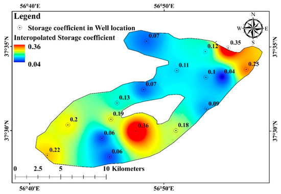
Figure 13.
The value of the interpolated storage coefficient of the Samalghan aquifer, using the ordinary Kriging method.
To study the aquifer behavior, the relationship between the DInSAR displacements for every extraction–recovery period concerning the distance to the wells was measured. For this purpose, in every extraction–recovery cycle at a radial distance varying from 250 to 4000 m from the observation wells (Figure 14), the average displacement was measured in the desired buffer area. Then, the maximum and minimum subsidence rates for the generated maps and their average were plotted on a graph. It was noted that the results were not significant and effective at a distance of 4000 m and they were rather homogeneous and intense from 1000 to 4000 m. On the other hand, at a radius of 1000 m, the effect of adjacent wells could be seen to some extent. Therefore, the greatest influence area of the aquifer exploitation is limited to the 1000 m-radius circle around the wells, and the values extracted from a radial distance of 4000 m were excluded from the analysis. The averages of the displacement data collected for each year were then plotted at a distance of 250 m, which was closest to each well, as shown in Figure 15.
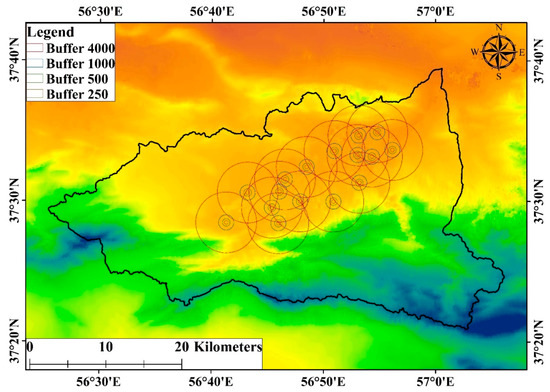
Figure 14.
Buffer areas with different radius values and locations around well fields in the study area on the displacement maps.
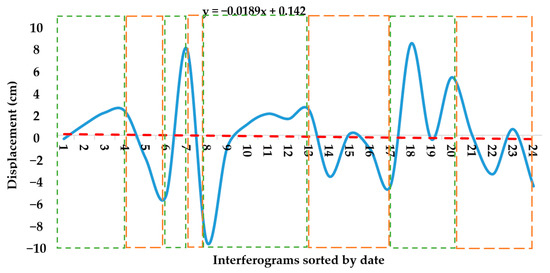
Figure 15.
Graph of average surface changes at a distance of 250 m from observation wells (green and orange-dashed rectangles representing recovery and extraction periods, respectively).
According to the trend of land surface changes in the study period (Figure 15), the whole time range was divided into four periods, including both uplift and subsidence. The data order in Figure 15 is ascending, with 1 representing the first interferogram produced in 2014, and 24 representing the last interferogram produced in 2020 (Table 5). A trend line was also fitted on the chart, representing the inelastic behavior in the region.
Table 5.
Interferogram ID and its corresponding number in Figure 15 X-axis.
The expected inelastic behavior in the region should be in accordance with the fitting line as represented in Figure 15. Due to the noncompliance of the aquifer system with this trend or behaving at the closest distance to this trend, it can be said that the behavior of the Samalghan aquifer might be elastic.
After the investigation of the selected periods, the relation between differential ground surface displacements and the duration of the extraction–recovery phases for every cycle was also analyzed. To reach this goal, the ratio of uplift–subsidence ratio (SR) and the cycle temporal ratio (TR) were calculated according to Table 6. The SR ratio represents the dependence between ground surface uplift during recovery and the subsidence that occurred in the extraction phase [29]. The results not only showed the highest average of subsidence in cycle 2, but also included the highest amount of uplift in the same period. The highest ratio of uplift to subsidence is in the fourth period, with a value of 1800% with a radius of 250 m around the wells. As is advised by [29], to achieve optimal aquifer management, the best time ratio is between 2 and 4. The closer the value obtained to this interval, the better the time frame for managing the area. Therefore, the first period has the best time interval, with a recovery period of 276 days and a subsidence period of 192 days. The third cycle also had a good value of TR, in which the recovery period was 444 days and the extraction period was 360 days. According to SR values, the smaller the time ratio in each period, the higher the monitored uplift to subsidence ratio. In agreement with the optimal number mentioned earlier, to reduce the damages caused by subsidence with proper management of water resources, for each year of uncontrolled extraction of plain resources, two years of plain could be considered as the recovery phase.
Table 6.
Average changes of the land surface in the four selected periods studied at different distances from observation wells, the ratio of uplift to subsidence values, and the ratio of uplift to subsidence phase.
According to Table 6, for cycle 1, ground surface subsidence related to the extraction phase represented the minimum value compared to the other cycles’ SR values of 32%, 20%, and 33% for 250 m, 500 m, and 1000 m from well fields, respectively. Meanwhile, the maximum TR value was represented in cycle 1, with the optimum amount of 1.43. In cycle 2, although the amount of uplift was on average about 3 times bigger than the phase 1 recovery, the value of subsidence compensated for both values of uplift in cycles 1 and 2. However, it was noticeable that the SR increased significantly. In the third cycle, the SR value decreased, while the TR value in this cycle rose. This procedure was reversed in the fourth cycle. While the time ratio decreased, the value of uplift increased significantly compared to subsidence in the extraction phase. The regional water company of North Khorasan proposed to rehabilitate water resources in 2016 and took action in 2018. Strict enforcement of groundwater extraction seems to have been effective in the study area.
Lastly, the stress–displacement relationship, which delivers a relationship between the measured displacement (ΔD) caused by a groundwater level fall (Δh), was computed for the water level drop–subsidence temporal series shown in Table 7 using Equation (1) [63,64]:
Table 7.
Computed elastic storage coefficient for wells shown in Figure 1.
The calculated value represents the deformability, and adopts different values with the stress rate according to the piezometric level [64]. When the stress induced by the hydraulic head variation overreaches the maximum pre-existing stress, as with preconsolidation stress, deformation rates could be largely high and irrecoverable in most cases due to the changes in arrangement and compaction of the soils. However, if induced stress does not exceed the preconsolidation stress, the deformations are much smaller and mostly elastic. This different soil behavior can be introduced to Equation 1 by assigning two different skeletal specific storages, elastic (Sske) and inelastic (Sskv), according to the state of stress concerning the preconsolidation stress.
In this work, the elastic storage coefficients Ske of the Samalghan aquifer were calculated for the period 2015–2020 using piezometric data for the 17 available wells where DInSAR retrieved deformations were also observed (Figure 16). These data applied for plotting the stress–strain curves that represent the relationship between piezometric level changes and aquifer system deformations, from which elastic storage coefficients were determined consisting of the slope of the branch of the stress–strain curve [29,64].
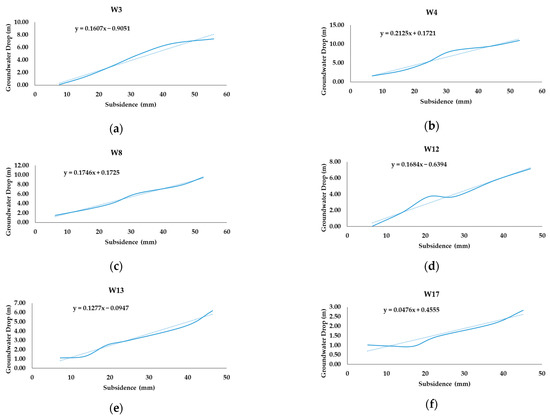
Figure 16.
Stress–strain analysis for wells W3 (a), W4 (b), W8 (c), W 12 (d), W13 (e), and W17 (f).
Figure 16 shows the stress–strain relationship at six well locations in the study area. Groundwater level drops define the stresses, and the ground displacements represent the vertical deformation of the aquifer system. The stress–strain trajectories during the period are similar in most of the wells. The Ske values of each well site obtained using the slope of the trendline for each well are shown in Table 7. Ske values vary from 3 × 10⁻⁶ at well 10 to 2.1 × 10⁻⁴ at well 4.
If the aquifer system is not stressed exceeding its preconsolidation stress, the Ske values are quite stable and independent of the considered time interval. The Ske computed values can be applied to estimate groundwater levels at well locations during the desired SAR acquisition time interval and compared with observed groundwater level values [3].
3.6. Suggestions
One of the complex issues that will arise with population growth in the future is the management of water resources in order to meet the demands and reduce the damage caused by the excessive extraction of groundwater.
Various factors have an impact on groundwater level drop [65], which can be controlled by proper management. First and foremost, one crucial step is increasing public awareness and attracting public participation [66] and implementing operational strategies. Water resources can be used optimally and these valuable resources can be protected. In order to manage the groundwater drop, several steps can be taken, some of which are addressed in this section.
3.6.1. Aquifer Conservation
The first action is the protection of groundwater aquifers. This is an important step to reduce the rate of groundwater depletion. There are several steps that can be taken to achieve this aim:
- Decentralization of exploitation wells [67];
- Increasing infiltration by restoring vegetation [68] in pastures;
- Construction control in aquifer recharge areas and preventing reduction of irrigation level;
- Increasing aquifer recharge through the use of injection wells [69], increasing infiltration of rivers and canals [70], flood infiltration in dried aqueducts, and recharging through infiltration of the surface water from natural pits.
3.6.2. Reduce Water Consumption
Reducing water consumption helps to reduce water loss in the region in several ways: first, by reducing groundwater extraction, and second, by reducing surface water consumption and increasing aquifer infiltration. There are several ways to do this:
- Explaining the leading problems and also increasing the level of awareness of consumers [71];
- Treatment of wastewater and effluents and their reuse [72];
- Improving soil conditions by using modern irrigation methods [73] and reducing evaporation;
- Reducing water transmission losses;
- Promoting greenhouse cultivation [74] in high-consumption areas;
- Promoting and developing hydroponics [75] and providing budgets for these facilities.
3.6.3. Soil Amendation
By improving collapsible soils, the development process of cracks in the Samalghan plain can be reduced. Due to the fact that the fractures in the plain have reached some roads and caused damage to them, it is possible to reduce further damages during the construction or repair of roads by using some techniques. Soil collection, replacement, and compaction; collection of moisture-sensitive soils; chemical stabilization by injection; and the use of piles or foundations are some of the steps that can be taken in this regard.
3.7. Geological Investigation
By comparing the results of annual cumulative displacement with the geological map (Figure 17), it is possible to identify the areas in which more subsidence has occurred. According to the given information in the previous study [42], the soil texture of the plain can be identified. Land deformation has occurred in different parts of the Samalghan plain, which is discussed as follows:
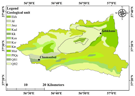
Figure 17.
Geological map of the Samalghan plain [42].
- East of the plain, on the Marl Formation, including fine sediments;
- North of the plain, on the Tirgan formation (Ktr), and composed of orbitoline limestone;
- Sarcheshmeh formation (Ksr) in the eastern Samalghan plain, containing marl (consisting of a high percentage of clay);
- The center of the plain where the aquifer is located, on new deposits (Qft2) composed of coarse- to fine-grained sediments including clay, sand, and silt, and Khangiran formation (Ekh), formed of sandstone;
- Some parts of eastern Chamanbid at a radius of 14 kms, and the south of Chamanbid at a distance of 2 km from the city on the Pliocene conglomerate (P1QC), which consists of sandstone and conglomerate, and some parts of Kalat Formation (Kk), including fine sand and erodible limestone;
- West of the plain at a distance of 4 km to the north of Chamanbid on a small part of the Jmz formation, composed of lime and dolomite;
- At 5 km to the northeast of Chamanbid, and southwest of Samalghan aquifer, which is located on a part of the Chamanbid formation (Jd).
The textures of the mentioned formations are mostly fine-grained and soluble rocks. Most of the constituent particles of these sections—lime, clay, and silty sediments—are fine-grained, which confirms that subsidence occurs mostly in fine-grained soils. Due to the clayey texture of the soil in most of these areas, the elastic behavior of the ground cannot be expected. Therefore, in these areas (Sanganeh, Marl, Qft2), it is not possible to propose new suggestions for the land recovery. In addition, the groundwater flow direction [39] is towards the center of the plain, and these areas outside the aquifer are not recharged at a high velocity; so in these areas, groundwater should be extracted under management.
According to the given information, from east to west and from south to north of the Samalghan aquifer, the soil texture varies from fine-grained to coarse-grained. For this reason, decision making in these sections should be different. In the western and northern aquifer, elastic behavior can be expected, so the subsidence can be recovered to an acceptable range by recharging this area or transferring surface water from the highlands to these areas. In contrast, the eastern and southern Samalghan aquifer, subsidence should be managed by overseeing and controlling the withdrawal from wells and managing the consumption of water resources, for example, reducing farmers’ water needs by modifying the cultivation pattern and increasing the irrigation system efficiency. To control subsidence in the Samalghan aquifer, the aquifer layers can be examined more closely using well log information, which will be available in extended studies.
3.8. Soft Soil Thickness
It is well-known that when the piezometric level falls, the land subsidence is greater if the accumulated compressible layer is thicker [76]. In this section, the distribution of soft soil thickness derived from boreholes located in the aquifer is compared to the land subsidence measured by DInSAR. The land subsidence in the Samalghan plain is developed in the sand, gravel, and clayey layer. Figure 18 represents the distribution of the mentioned soft soil layer existing in the Samalghan aquifer overlayed with the slope map. The clayey layer is one of the biggest contributors to land subsidence. As can be seen from Figure 18, the layer thickness from the surface ranges between ~30 to 140 m, and as shown in the deformation maps, all of these areas are affected by land subsidence.
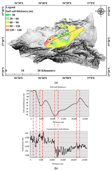
Figure 18.
Soft soil thickness map of the Samalghan plain (a); the line shows the section used for investigating the soft soil section along the southwest–northeast direction (b).
For better investigation, a cross section was employed to better interpret the relation between the soft soil and the deformation. Although there is some correlation between these two (as shown in red boxes in some places), there are some areas that are not completely affected by soft soil. For example, in the first box, the figure for accumulated subsidence reached 40 cm, where the soil thickness increased to its highest value, and in the second box, the accumulated subsidence decreased to approximately 25 cm as the thickness decreased to just below 70 m. However, this trend is not always the same along the area, e.g., in the distance of 15000–2000 m, which shows that the subsidence is not completely affected by the soil thickness. Although subsidence affected some areas according to their thickness, the relation between the subsidence and the groundwater drop was stronger in the deformed area.
4. Conclusions
Most of the previous studies have illustrated plastic or elastoplastic deformation in aquifers [4,6,9,11]. Overexploitation and continuous piezometric level decline [7] act together with seasonal variations [11] as the main driving factors of land subsidence. These variations are usually the reason for continuous plastic deformation and cyclic elastic deformations in aquifers [29].
The present study aimed to monitor land subsidence using the Sentinel-1 radar images in Samalghan plain and investigate its relationship with changes in groundwater level and aquifer behavior. The spatial and temporal evolution of ground surface displacement was evaluated using radar interferometry by processing datasets of Sentinel-1 SLC from November 2014 to November 2020, with results showing that subsidence occurred over most of the Samalghan plain, while in a few areas uplift was also observed in one or more years. It shows that the aquifer behavior showed an elastic deformation in some areas, but in other parts of the region, plastic deformation was detected. With the examination of groundwater level changes in Samalghan plain and land deformation in this area, it can be concluded that the subsidence in this plain is affected by groundwater depletion and uncontrolled extraction from the aquifer. The study of the aquifer interaction in the area concerning the variation of land deformation caused by changes in the groundwater level represents an elastic behavior of the land in the Samalghan aquifer and around Chamanbid city, and the inelastic behavior of the land surface in other parts of the plain. It is undeniable that understanding the land surface response to water level decline is essential in arid and semiarid areas to reduce damage and achieve sustainable water resource management. These results showed that the quasi-elastic aquifer deformational behavior is influenced by groundwater withdrawal in Samalghan plain. Applying groundwater management exploitation seems reasonable because the piezometric level in wells is mostly recovered after the extraction periods. To illustrate, it can be advised that after 1–2 years of overexploitation, the aquifer should enter 2–4 years of recovery. In addition, the identified displacements show a modest subsidence phenomenon influencing a broad area. With reference to the continuous groundwater depletion in the Samalghan plain, both aquifer conservation and reducing water consumption would alleviate the current situation. However, some actions could be taken specifically in areas pursuant to their subsidence situation. We advise that according to the subsidence pattern and the geological structures (Figure 7 and Figure 17), proposed methods of reducing water consumption should be applied to the Ktr, Ekh, and Mur sections to manage water consumption. Furthermore, aquifer conservation would be practical in some parts of the PlQC, Kad, Jmz, Qft2, and northern parts of Ktr geological sections. The investigation of the relationship between land subsidences showed that although there is a small correlation between the soft soil thickness and the land deformation, the subsidence in this area is mostly affected by the groundwater level variations.
Author Contributions
For research contributions, Fatemeh Rafiei performed data processing and the first drafting of the manuscript; Saeid Gharechelou methodologically advised, investigated, and validated the result and edited the manuscript; Saeed Golian supervised; and Brian Alan Johnson revised the final manuscript grammatically and technically. All authors have read and agreed to the published version of the manuscript.
Funding
This research received no external funding.
Data Availability Statement
Data are available on request.
Acknowledgments
The authors acknowledge the support of the Regional Water Authority of North Khorasan province of Iran for groundwater data and some water resources reports sharing. We would also like to thank the experts for their contribution in progressing this study.
Conflicts of Interest
The authors declare no conflict of interest.
References
- Custodio, E. Aquifer overexploitation: What does it mean? Hydrogeol. J. 2002, 10, 254–277. [Google Scholar] [CrossRef]
- Famiglietti, J.S. The global groundwater crisis. Nat. Clim. Chang. 2014, 4, 945–948. [Google Scholar] [CrossRef]
- Béjar-Pizarro, M.; Ezquerro, P.; Herrera, G.; Tomás, R.; Guardiola-Albert, C.; Hernández, J.M.R.; Fernández, M.; Miguel, M.; Martínez, R. Mapping groundwater level and aquifer storage variations from InSAR measurements in the Madrid aquifer, Central Spain. J. Hydrol. 2017, 547, 678–689. [Google Scholar] [CrossRef]
- Chitsazan, M.; Rahmani, G.; Ghafoury, H. Investigation of subsidence phenomenon and impact of groundwater level drop on alluvial aquifer, case study: Damaneh-Daran plain in west of Isfahan province, Iran. Model. Earth Syst. Environ. 2020, 6, 1145–1161. [Google Scholar] [CrossRef]
- Bhattarai, R.; Alifu, H.; Maitiniyazi, A.; Kondoh, A. Detection of land subsidence in Kathmandu Valley, Nepal, using DInSAR technique. Land 2017, 6, 39. [Google Scholar] [CrossRef]
- Bai, Z.; Wang, Y.; Balz, T. Beijing Land Subsidence Revealed Using PS-InSAR with Long Time Series TerraSAR-X SAR Data. Remote Sens. 2022, 14, 2529. [Google Scholar] [CrossRef]
- Gao, M.; Gong, H.; Chen, B.; Li, X.; Zhou, C.; Shi, M.; Yuan, S.; Zheng, C.; Duan, G. Regional land subsidence analysis in eastern Beijing plain by insar time series and wavelet transforms. Remote Sens. 2018, 10, 365. [Google Scholar] [CrossRef]
- Cigna, F.; Tapete, D. Present-day land subsidence rates, surface faulting hazard and risk in Mexico City with 2014–2020 Sentinel-1 IW InSAR. Remote Sens. Environ. 2021, 253, 112161. [Google Scholar] [CrossRef]
- Miller, M.M.; Jones, C.E.; Sangha, S.S.; Bekaert, D. Rapid drought-induced land subsidence and its impact on the California aqueduct. Remote Sens. Environ. 2020, 251, 112063. [Google Scholar] [CrossRef]
- Braun, A.; Hochschild, V.; Pham, G.T.; Nguyen, L.H.K.; Bachofer, F. Linking land subsidence to soil types within Hue city in Central Vietnam. J. Vietnam. Environ. 2020, 12, 1–6. [Google Scholar] [CrossRef]
- Rezaei, A.; Mousavi, Z. Characterization of land deformation, hydraulic head, and aquifer properties of the Gorgan confined aquifer, Iran, from InSAR observations. J. Hydrol. 2019, 579, 124196. [Google Scholar] [CrossRef]
- Yastika, E.; Shimizu, N.; Abidin, H.Z. Monitoring of long-term land subsidence from 2003 to 2017 in coastal area of Semarang, Indonesia by SBAS DInSAR analyses using Envisat-ASAR, ALOS-PALSAR, and Sentinel-1A SAR data. Adv. Space Res. 2019, 63, 1719–1736. [Google Scholar] [CrossRef]
- Gharechelou, S.; Akbari Ghoochani, H.; Golian, S.; Ganji, K. Evaluation of land subsidence relationship with groundwater depletion using Sentinel-1 and ALOS-1 radar data (Case study: Mashhad plain). J. GIS RS for Nat. Res. 2021, 12, 11–14. Available online: http://dorl.net/dor/20.1001.1.26767082.1400.12.3.3.8 (accessed on 1 October 2021). (In Persian).
- Mesgaran, M.B.; Madani, K.; Hashemi, H.; Azadi, P. Iran’s land suitability for agriculture. Sci. Rep. 2017, 7, 7670. [Google Scholar] [CrossRef]
- Mohammady, M.; Pourghasemi, H.R.; Amiri, M.; Tiefenbacher, J. Spatial modeling of susceptibility to subsidence using machine learning techniques. Stoch. Environ. Res. Risk Assess. 2021, 35, 1689–1700. [Google Scholar] [CrossRef]
- Sayyaf, M.; Mahdavi, M.; Barani, O.R.; Feiznia, S.; Motamedvaziri, B. Simulation of land subsidence using finite element method: Rafsanjan plain case study. Nat. Hazards 2014, 72, 309–322. [Google Scholar] [CrossRef]
- Dyskin, A.V.; Pasternak, E.; Shapiro, S.A. Fracture mechanics approach to the problem of subsidence induced by resource extraction. Eng. Fract. Mech. 2020, 236, 107173. [Google Scholar] [CrossRef]
- Abou Zaki, N.; Torabi Haghighi, A.M.; Rossi, P.J.; Tourian, M.; Kløve, B. Monitoring groundwater storage depletion using gravity recovery and climate experiment (GRACE) data in Bakhtegan Catchment, Iran. Water 2019, 11, 1456. [Google Scholar] [CrossRef]
- Wang, D.; Li, M.; Chen, J.; Xia, X.; Zhang, Y. Numerical study on groundwater drawdown and deformation responses of multi-layer strata to pumping in a confined aquifer. J. Shanghai Jiaotong Univ. 2019, 24, 287–293. [Google Scholar] [CrossRef]
- Poland, J.F.; Davis, G.H. Land Subsidence Due to Withdrawal of Fluids. In Reviews in Engineering Geology; Varnes, D.J., Kiersch, G., Eds.; Geological Society of America: Onslow Beach, NC, USA, 1969; Volume 2, pp. 187–269. [Google Scholar] [CrossRef]
- Guzy, A.; Malinowska, A.A. State of the art and recent advancements in the modelling of land subsidence induced by groundwater withdrawal. Water 2020, 12, 2051. [Google Scholar] [CrossRef]
- Wilson, A.M.; Gorelick, S. The effects of pulsed pumping on land subsidence in the Santa Clara Valley, California. J. Hydrol. 1996, 174, 375–396. [Google Scholar] [CrossRef]
- Zhang, Y.; Wu, J.; Xue, Y.; Wang, Z.; Yao, Y.; Yan, X.; Wang, H. Land subsidence and uplift due to long-term groundwater extraction and artificial recharge in Shanghai, China. Hydrogeol. J. 2015, 23, 1851–1866. [Google Scholar] [CrossRef]
- Hammond, W.C.; Burgette, R.J.; Johnson, K.M.; Blewitt, G. Uplift of the western transverse ranges and Ventura area of Southern California: A four-technique geodetic study combining GPS, InSAR, leveling, and tide gauges. J. Geophys. Res. Solid Earth 2018, 123, 836–858. [Google Scholar] [CrossRef]
- Hu, X.; Lu, Z.; Wang, T. Characterization of hydrogeological properties in salt lake valley, Utah, using InSAR. J. Geophys. Res. Earth Surf. 2018, 123, 1257–1271. [Google Scholar] [CrossRef]
- Galloway, D.L.; Burbey, T.J. Regional land subsidence accompanying groundwater extraction. Hydrogeol. J. 2011, 19, 1459–1486. [Google Scholar] [CrossRef]
- Khan, S.D.; Huang, Z.; Karacay, A. Study of ground subsidence in northwest Harris county using GPS, LiDAR, and InSAR techniques. Nat. Hazards 2014, 73, 1143–1173. [Google Scholar] [CrossRef]
- Bürgmann, R.; Rosen, A.; Fielding, E.J. Synthetic aperture radar interferometry to measure Earth’s surface topography and its deformation. Annu. Rev. Earth Planet Sci. 2000, 28, 169–209. [Google Scholar] [CrossRef]
- Ezquerro, P.; Herrera, G.; Marchamalo, M.; Tomás, R.; Béjar-Pizarro, M.; Martínez, R. A quasi-elastic aquifer deformational behavior: Madrid aquifer case study. J. Hydrol. 2014, 519, 1192–1204. [Google Scholar] [CrossRef]
- Sui, L.; Ma, F.; Chen, N. Mining subsidence prediction by combining support vector machine regression and interferometric synthetic aperture radar data. ISPRS Int. J. Geo-Inf. 2020, 9, 390. [Google Scholar] [CrossRef]
- Martins, B.H.; Suzuki, M.; Yastika, E.; Shimizu, N. Ground surface deformation detection in complex landslide area—Bobonaro, Timor-Leste—Using SBAS DinSAR, UAV photogrammetry, and field observations. Geosciences 2020, 10, 245. [Google Scholar] [CrossRef]
- Braun, A. Retrieval of digital elevation models from Sentinel-1 radar data–open applications, techniques, and limitations. Open Geosci. 2021, 13, 532–569. [Google Scholar] [CrossRef]
- Raspini, F.; Bardi, F.; Bianchini, S.; Ciampalini, A.; Del Ventisette, C.; Farina, P.; Ferrigno, F.; Solari, L.; Casagli, N. The contribution of satellite SAR-derived displacement measurements in landslide risk management practices. Nat. Hazards 2017, 86, 327–351. [Google Scholar] [CrossRef]
- Fárová, K.; Jelének, J.; Kopačková-Strnadová, V.; Kycl, P. Comparing DInSAR and PSI techniques employed to Sentinel-1 data to monitor highway stability: A case study of a massive Dobkovičky landslide, Czech Republic. Remote Sens. 2019, 11, 2670. [Google Scholar] [CrossRef]
- Cigna, F.; Tapete, D. Satellite InSAR survey of structurally-controlled land subsidence due to groundwater exploitation in the Aguascalientes Valley, Mexico. Remote Sens. Environ. 2021, 254, 112254. [Google Scholar] [CrossRef]
- Orhan, O.; Oliver-Cabrera, T.; Wdowinski, S.; Yalvac, S.; Yakar, M. Land subsidence and its relations with sinkhole activity in Karapınar region, Turkey: A multi-sensor InSAR time series study. Sensors 2021, 21, 774. [Google Scholar] [CrossRef]
- Del Soldato, M.; Solari, L.; Raspini, F.; Bianchini, S.; Ciampalini, A.; Montalti, R.; Ferretti, A.; Pellegrineschi, V.; Casagli, N. Monitoring ground instabilities using SAR satellite data: A practical approach. ISPRS Int. J. Geo-Inf. 2019, 8, 307. [Google Scholar] [CrossRef]
- Khosropanah, E.; Karami, G.; Jeyhooni, S. Effects of the excessive withdrawals of groundwater and subsidence in the Semalghan plain. In Proceedings of the 7th Iranian Conference of Engineering Geology and the Environment, Shahrud, Iran, 5 September 2011. (In Persian). [Google Scholar]
- Rafiee, F.; Gharechelou, S.; Golian, S.; Nozarpour, N. Recharge and Discharge Zones Identification using GIS (Case study: Semalghan plain). In Proceedings of the 12th International Congress on Civil Engineering, Mashhad, Iran, 12–14 July 2021. [Google Scholar]
- Nasiri, S.; Ansari, H.; Ziaei, A.N. Simulation of water balance equation components using SWAT model in Samalqan Watershed (Iran). Arab. J. Geosci. 2020, 13, 421. [Google Scholar] [CrossRef]
- Singh, N.S.; Sharma, R.; Parween, T.; Patanjali, K. Modern Age Environmental Problems and their Remediation. In Pesticide Contamination and Human Health Risk Factor; Oves, M., Zain Khan, M., Ismail, I.M.I., Eds.; Springer: Cham, Switzerland, 2018; pp. 49–68. [Google Scholar] [CrossRef]
- Ajam, H.; Mohammadzadeh, H.; Karami, Q.; Kazemi Gelian, R. Investigating of Samalqan aquifer groundwater quality base on underground variations of alluvial and rock facies. Sci Semiannu. J. Sediment. Facies 2018, 10, 291–310. (In Persian) [Google Scholar] [CrossRef]
- Liu, Z.; Liu, W.; Massoud, E.; Farr, T.G.; Lundgren, P.; Famiglietti, J.S. Monitoring groundwater change in California’s central valley using sentinel-1 and grace observations. Geosciences 2019, 9, 436. [Google Scholar] [CrossRef]
- Bui, L.K.; Le, V.; Dao, D.; Long, N.Q.; Pham, H.V.; Tran, H.H.; Xie, L. Recent land deformation detected by Sentinel-1A InSAR data (2016–2020) over Hanoi, Vietnam, and the relationship with groundwater level change. Gisci. Remote Sens. 2021, 58, 161–179. [Google Scholar] [CrossRef]
- Koukouvelas, I.; Mpresiakas, A.; Sokos, E.; Doutsos, T. The tectonic setting and earthquake ground hazards of the 1993 Pyrgos earthquake, Peloponnese, Greece. J. Geol. Soc. 1996, 153, 39–49. [Google Scholar] [CrossRef]
- Chen, B.; Gong, H.; Chen, Y.; Lei, K.; Zhou, C.; Si, Y.; Li, X.; Pan, Y.; Gao, M. Investigating land subsidence and its causes along Beijing high-speed railway using multi-platform InSAR and a maximum entropy model. Int. J. Appl. Earth Obs. Geoinf. 2021, 96, 102284. [Google Scholar] [CrossRef]
- Khorrami, M.; Hatami, M.; Alizadeh, B.; Khorrami, H.; Rahgozar, P.; Flood, I. Impact of ground subsidence on groundwater quality: A case study in Los Angeles, California. In Proceedings of the Computing in Civil Engineering 2019: Smart Cities, Sustainability, and Resilience, Atlenta, GA, USA, 17–19 June 2019; American Society of Civil Engineers: Reston, VA, USA, 2019; pp. 162–170. [Google Scholar]
- Veci, L. TOPS Interferometry Tutorial. Sentinel-1 Toolbox; Array Systems Computing Inc. and ESA, 2015. Available online: http://step.esa.int/docs/tutorials/S1TBX%20Stripmap%20Interferometry%20with%20Sentinel-1%20Tutorial.pdf (accessed on 27 September 2018).
- Sansosti, E.; Berardino, P.; Manunta, M.; Serafino, F.; Fornaro, G. Geometrical SAR image registration. IEEE Trans. Geosci. Remote Sens. 2006, 44, 2861–2870. [Google Scholar] [CrossRef]
- Kelany, K.A.H.; Baniasadi, A.; Dimopoulos, N.; Gara, M. Improving InSAR Image Quality and Co-Registration through CNN-Based Super-Resolution. In Proceedings of the IEEE International Symposium on Circuits and Systems (ISCAS), Seville, Spain, 28 September 2020; pp. 1–5. [Google Scholar]
- Fattahi, H.; Agram, P.; Simons, M. A network-based enhanced spectral diversity approach for TOPS time-series analysis. IEEE Trans. Geosci. Remote Sens. 2016, 55, 777–786. [Google Scholar] [CrossRef]
- Wegmttller, U.; Strozzi, T.; Werner, C.; Wiesmann, A.; AG, G.R.S. Sar interferometry for topographic mapping and surface deformation monitoring. FJP 2002, 18, 24–32. [Google Scholar]
- Tolomei, C.; Caputo, R.; Polcari, M.; Famiglietti, N.A.; Maggini, M.; Stramondo, S. The use of interferometric synthetic aperture radar for isolating the contribution of major shocks: The case of the thessaly, Greece, seismic sequence. Geosciences 2021, 11, 191. [Google Scholar] [CrossRef]
- Ai, B.; Liu, K.; Li, X.; Li, D.H. Flat-earth phase removal algorithm improved with frequency information of interferogram. In Proceedings of the Geoinformatics and Joint Conference on GIS and Built Environment: Classification of Remote Sensing Images, Guangzhou, China, 7 November 2008; Volume 7147, pp. 418–427. [Google Scholar] [CrossRef]
- Xu, B.; Li, Z.; Zhu, Y.; Shi, J.; Feng, G. SAR interferometric baseline refinement based on flat-earth phase without a ground control point. Remote Sens. 2020, 12, 233. [Google Scholar] [CrossRef]
- Goldstein, R.M.; Werner, C.L. Radar interferogram filtering for geophysical applications. Geophys. Res. Lett. 1998, 25, 4035–4038. [Google Scholar] [CrossRef]
- Chen, C.W.; Zebker, H.A. Two-dimensional phase unwrapping with statistical models for nonlinear optimization. In Proceedings of the IGARSS 2000—IEEE 2000 International Geoscience and Remote Sensing Symposium. Taking the Pulse of the Planet: The Role of Remote Sensing in Managing the Environment. Proceedings (Cat. No. 00CH37120), Honolulu, HI, USA, 6 August 2000; Volume 7, pp. 3213–3215. [Google Scholar] [CrossRef]
- Huang, Q.; Zhou, H.; Dong, S.; Xu, S. Parallel branch-cut algorithm based on simulated annealing for large-scale phase unwrapping. IEEE Trans. Geosci. Remote Sens. 2015, 53, 3833–3846. [Google Scholar] [CrossRef]
- Johnson, B.; Tateishi, R.; Kobayashi, T. Remote sensing of fractional green vegetation cover using spatially-interpolated endmembers. Remote Sens. 2012, 4, 2619–2634. [Google Scholar] [CrossRef]
- Maghsoudi, Y.; Amani, R.; Ahmadi, H. A study of land subsidence in west of Tehran using Sentinel-1 data and permanent scatterer interferometric technique. Arab. J. Geosci. 2021, 14, 30. [Google Scholar] [CrossRef]
- Sadeghi, Z.; Veldan Zoj, M.J.; Dehghani, M. Introduction and comparison of two radar interferometry methods based on permanent scatterer to measure land subsidence (Case study: Southwest of Tehran plain). Iran. J. Remote Sens. GIS 2012, 4, 97–110. (In Persian) [Google Scholar]
- Bonì, R.; Cigna, F.; Bricker, S.; Meisina, C.; McCormack, H. Characterisation of hydraulic head changes and aquifer properties in the London Basin using Persistent Scatterer Interferometry ground motion data. J. Hydrol. 2016, 540, 835–849. [Google Scholar] [CrossRef]
- Navarro-Hernández, M.I.; Tomás, M.; Lopez-Sanchez, J.M.; Cárdenas-Tristán, A.; Mallorquí, J.J. Spatial analysis of land subsidence in the San Luis Potosi valley induced by aquifer overexploitation using the coherent pixels technique (CPT) and sentinel-1 InSAR observation. Remote Sens. 2020, 12, 3822. [Google Scholar] [CrossRef]
- Tomás, R.; Herrera, G.; Delgado, J.; Lopez-Sanchez, J.M.; Mallorquí, J.J.; Mulas, J. A ground subsidence study based on DInSAR data: Calibration of soil parameters and subsidence prediction in Murcia City (Spain). Eng. Geol. 2010, 111, 19–30. [Google Scholar] [CrossRef]
- Dinh, B.H.; Go, G.H.; Kim, Y.S. Performance of a horizontal heat exchanger for ground heat pump system: Effects of groundwater level drop with soil–water thermal characteristics. Appl. Therm. Eng. 2021, 195, 117203. [Google Scholar] [CrossRef]
- Samani, S. Analyzing the groundwater resources sustainability management plan in Iran through comparative studies. Groundw. Sustain. Dev. 2021, 12, 100521. [Google Scholar] [CrossRef]
- Joshi, D.; Kulkarni, H.; Aslekar, U. Bringing aquifers and communities together: Decentralised groundwater governance in rural India. In Proceedings of the Water Governance: Challenges and Prospects, Singapore, 1 February 2019. [Google Scholar] [CrossRef]
- Lozano-Baez, S.E.; Cooper, M.; Meli, P.; Ferraz, S.F.; Rodrigues, R.R.; Sauer, T.J. Land restoration by tree planting in the tropics and subtropics improves soil infiltration, but some critical gaps still hinder conclusive results. For. Ecol. Manag. 2019, 444, 89–95. [Google Scholar] [CrossRef]
- Parker, A.L.; Pigois, J.P.; Filmer, M.S.; Featherstone, W.E.; Timms, N.E.; Penna, N.T. Land uplift linked to managed aquifer recharge in the Perth Basin, Australia. Int. J. Appl. Earth Obs. Geoinf. 2021, 105, 102637. [Google Scholar] [CrossRef]
- Villeneuve, S.; Cook, G.; Shanafield, M.; Wood, C.; White, N. Groundwater recharge via infiltration through an ephemeral riverbed, central Australia. J. Arid Environ. 2015, 117, 47–58. [Google Scholar] [CrossRef]
- Stavenhagen, M.; Buurman, J.; Tortajada, C. Saving water in cities: Assessing policies for residential water demand management in four cities in Europe. Cities 2018, 79, 187–195. [Google Scholar] [CrossRef]
- Zhang, H.; Xu, Y.; Kanyerere, T. A review of the managed aquifer recharge: Historical development, current situation and perspectives. Phys. Chem. Earth 2020, 118, 102887. [Google Scholar] [CrossRef]
- Porhemmat, J.; Nakhaei, M.; Dadgar, M.A.; Biswas, A. Investigating the effects of irrigation methods on potential groundwater recharge: A case study of semiarid regions in Iran. J. Hydrol. 2018, 565, 455–466. [Google Scholar] [CrossRef]
- Raeisi, L.G.; Morid, S.; Delavar, M.; Srinivasan, R. Effect and side-effect assessment of different agricultural water saving measures in an integrated framework. Agric. Water Manag. 2019, 223, 105685. [Google Scholar] [CrossRef]
- Edgerton, C.; Estrada, A.; Fairchok, K.; Parker, M.T.; Jezak, A.; Pavelka, C.; Lee, H.; Doyle, L.; Feldmeth, A. Addressing water insecurity with a greywater hydroponics system in South Africa. In Proceedings of the IEEE Global Humanitarian Technology Conference (GHTC), Seattle, WA, USA, 29 October–1 November 2020; pp. 1–4. [Google Scholar] [CrossRef]
- Chen, M.; Tomás, R.; Li, Z.; Motagh, M.; Li, T.; Hu, L.; Gong, H.; Li, X.; Yu, J.; Gong, X. Imaging land subsidence induced by groundwater extraction in Beijing (China) using satellite radar interferometry. Remote Sens. 2016, 8, 468. [Google Scholar] [CrossRef]
Publisher’s Note: MDPI stays neutral with regard to jurisdictional claims in published maps and institutional affiliations. |
© 2022 by the authors. Licensee MDPI, Basel, Switzerland. This article is an open access article distributed under the terms and conditions of the Creative Commons Attribution (CC BY) license (https://creativecommons.org/licenses/by/4.0/).