
Prediction of Urban Sprawl by Integrating Socioeconomic Factors in the Batticaloa Municipal Council, Sri Lanka


Abstract
:1. Introduction
2. Materials and Methods
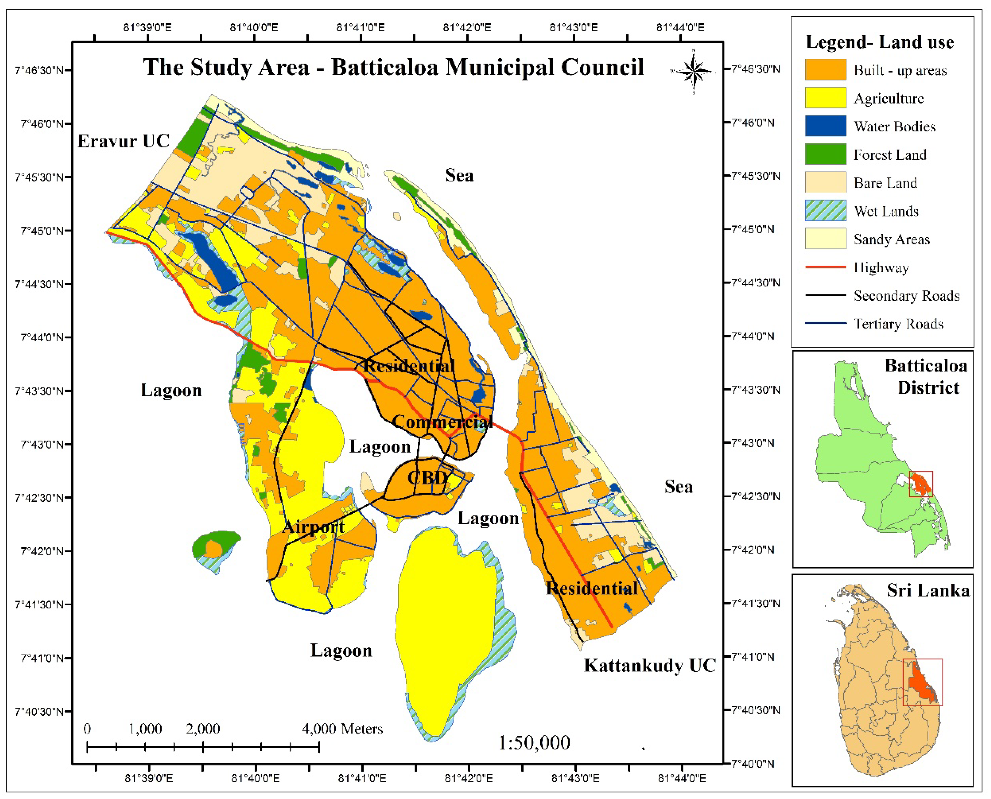
2.1. Study Area
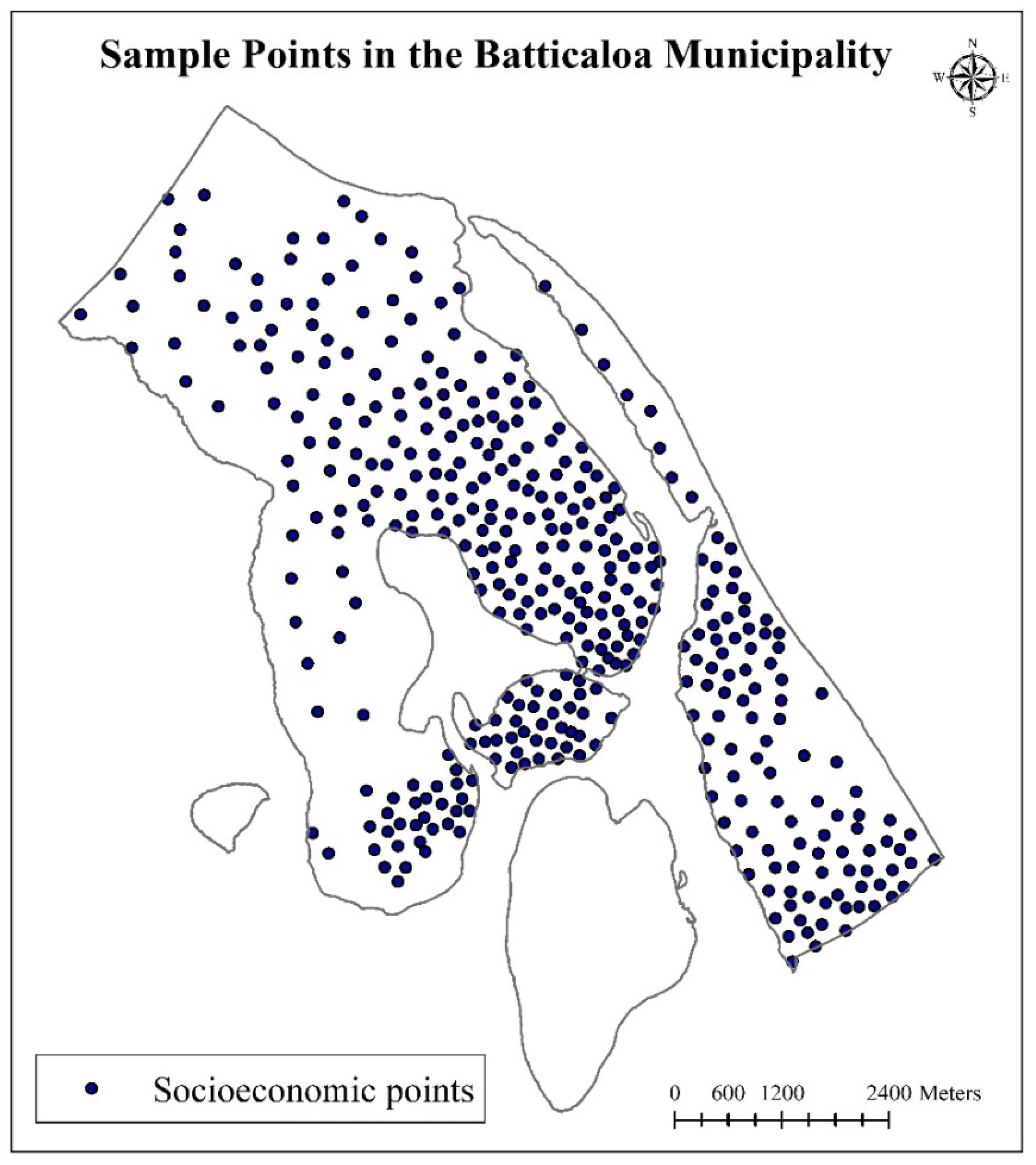
2.2. Data Source
2.3. Data Analysis
2.3.1. Normalized Difference Built-Up Index (NDBI)
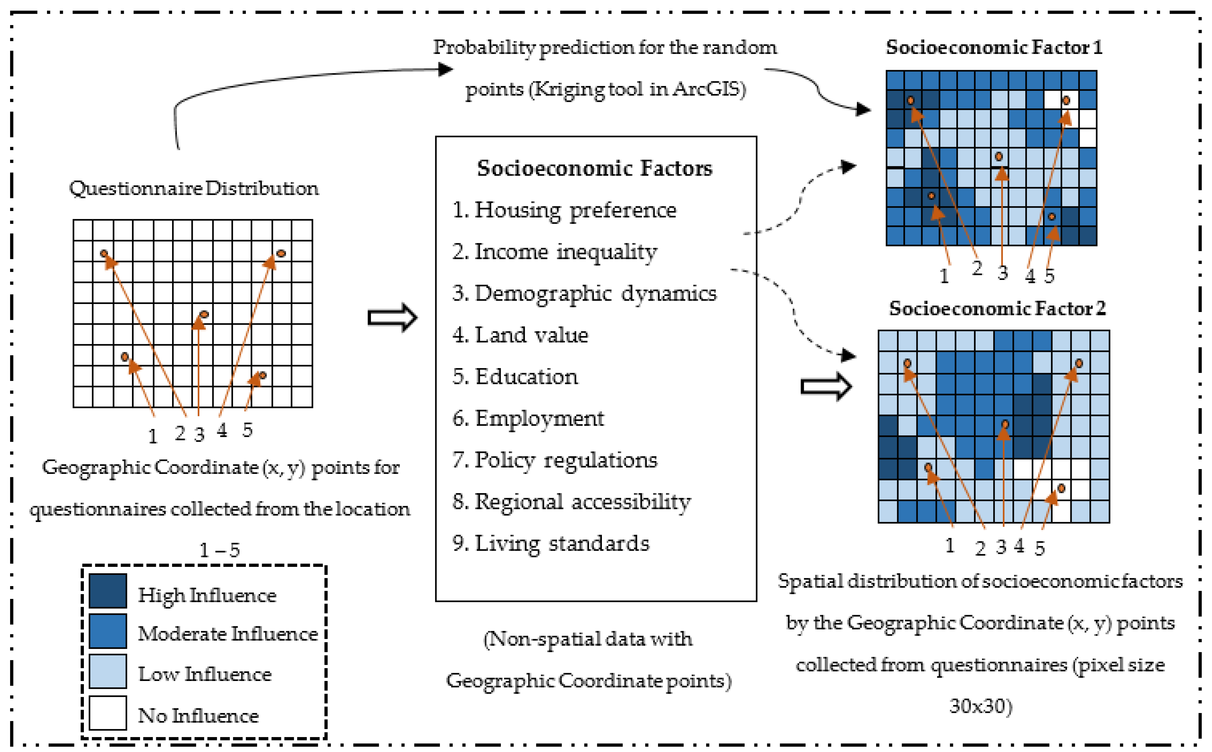
2.3.2. Socioeconomic Data Transformation
2.3.3. Cramer’s V Test
2.3.4. Sub Model: Logistic Regression
2.3.5. CA-Markov Model
2.3.6. Model Validation
3. Results and Discussion
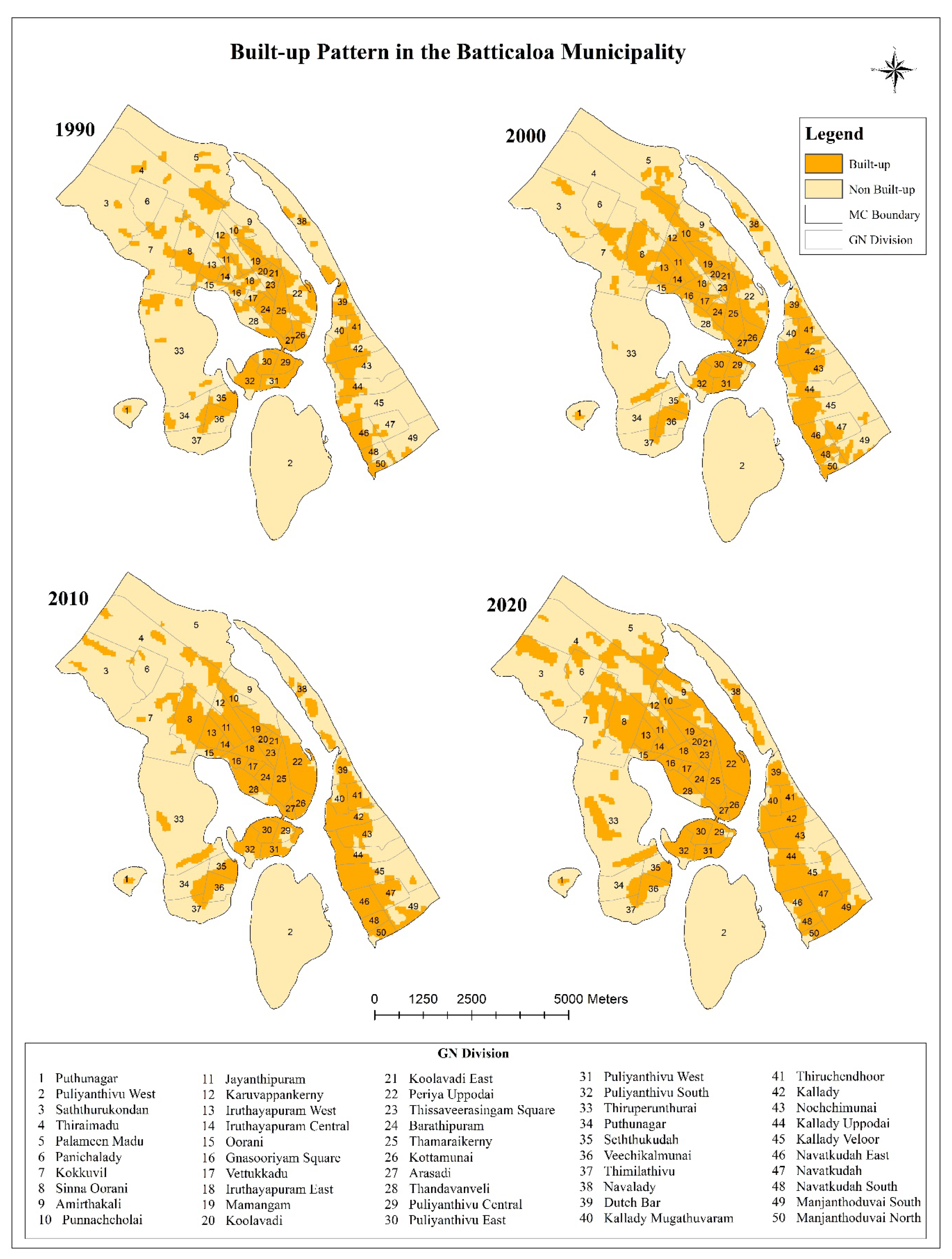
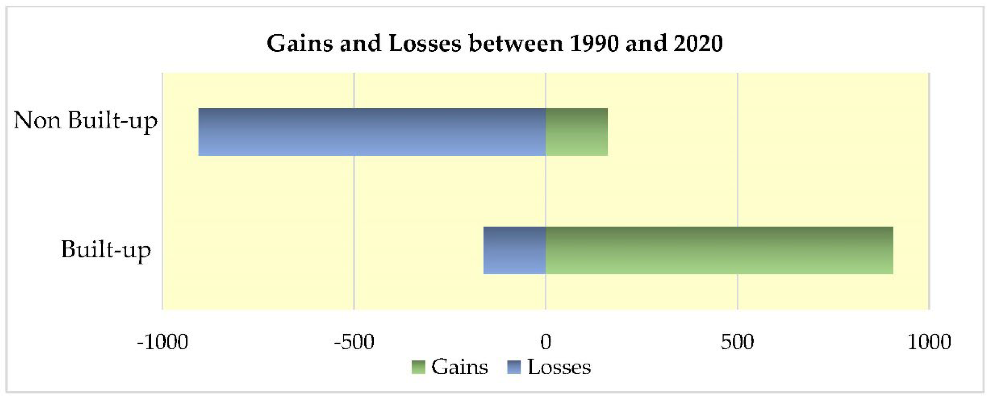
3.1. Built-Up Pattern
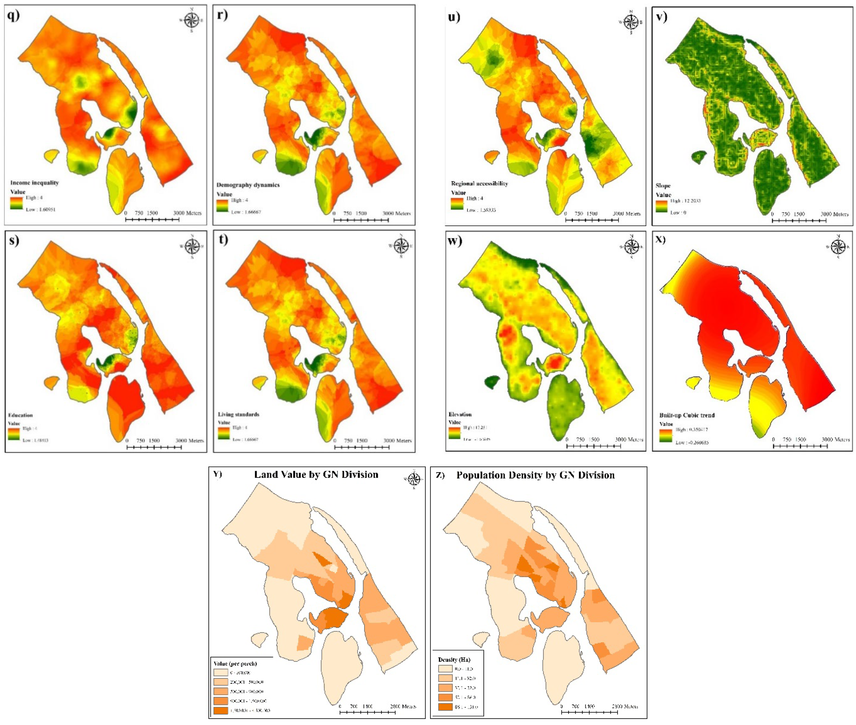
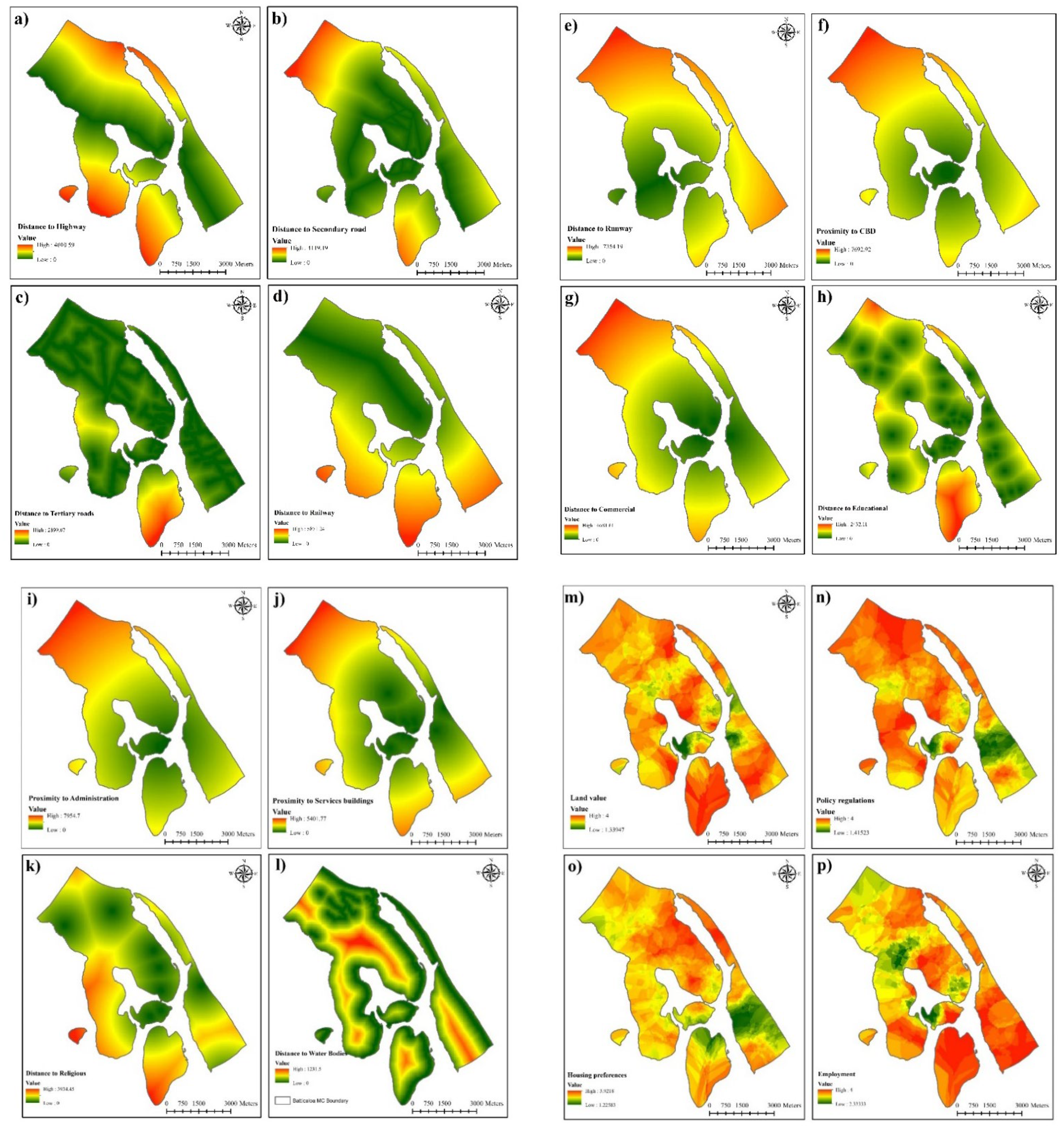
3.2. Selection of Drivers’ Variables
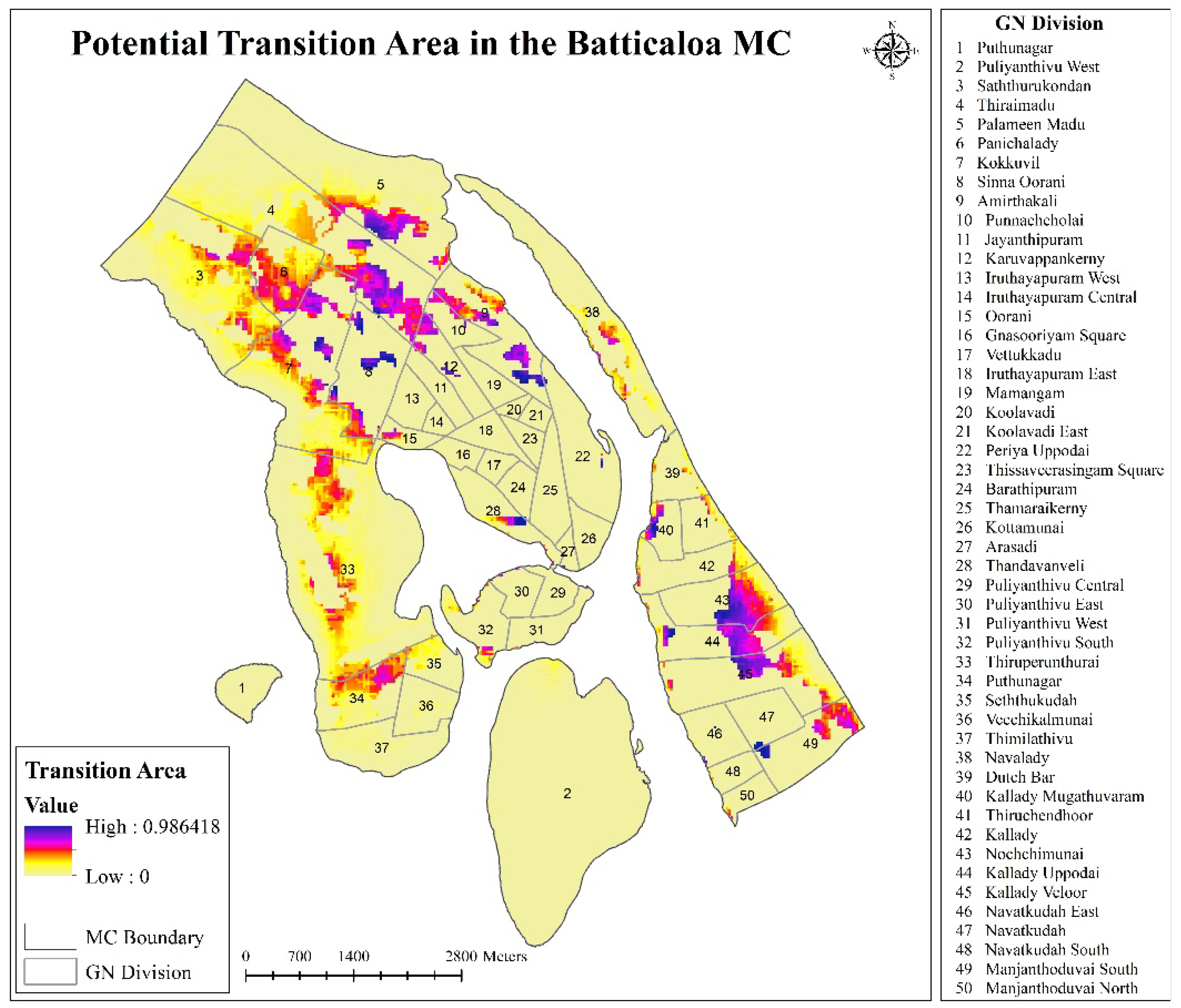
3.3. Transition Potentials
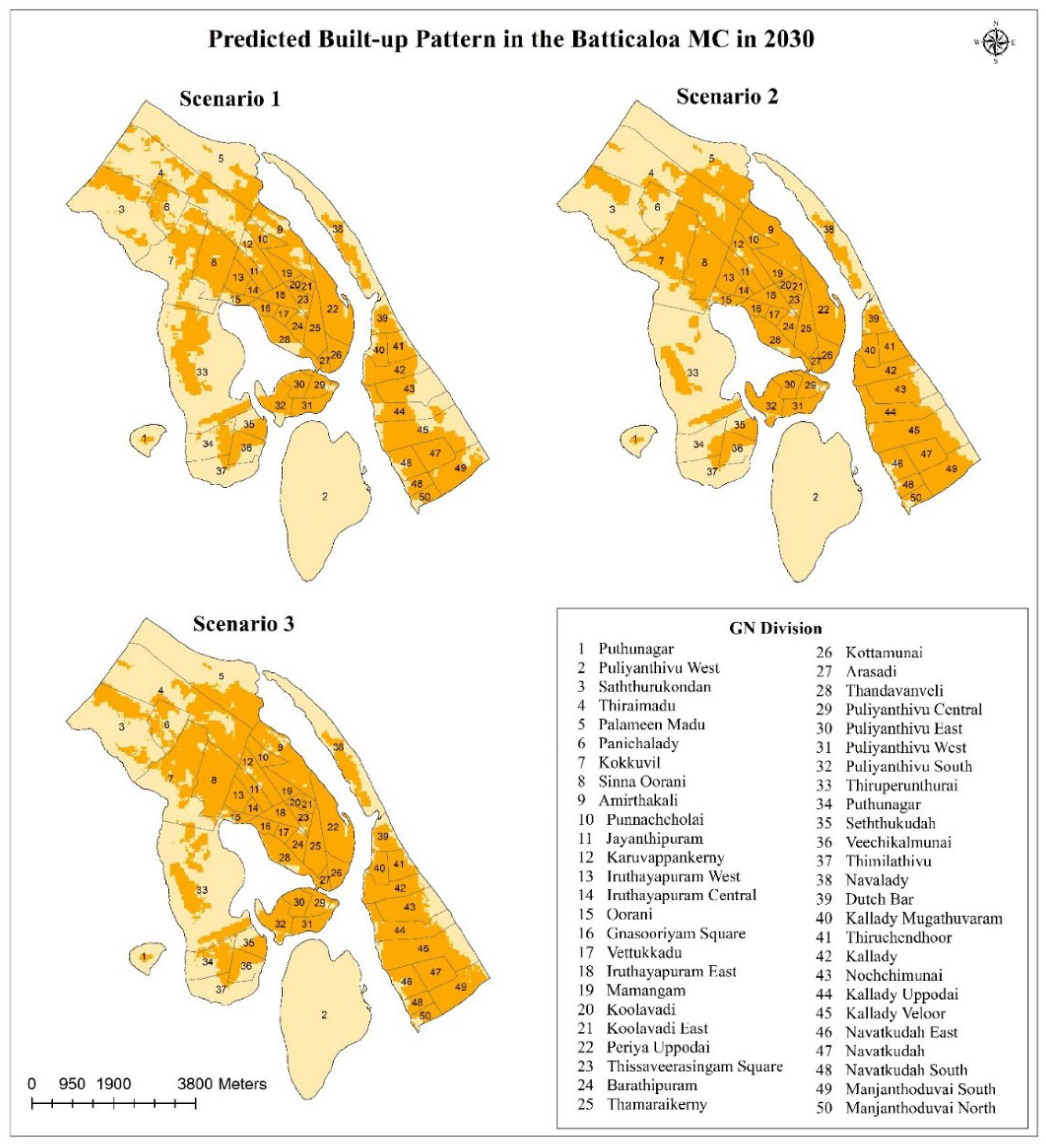
3.4. Urban Sprawl Prediction in 2030
4. Conclusions
Author Contributions
Funding
Institutional Review Board Statement
Informed Consent Statement
Data Availability Statement
Acknowledgments
Conflicts of Interest
References
- Grigorescu, I.; Kucsicsa, G.; Mitrică, B. Assessing spatio-temporal dynamics of urban sprawl in the Bucharest metropolitan area over the last century. Land Use Cover. Changes Sel. Reg. World 2015, 10, 19–27. [Google Scholar]
- Chettry, V.; Surawar, M. Assessment of urban sprawl characteristics in Indian cities using remote sensing: Case studies of Patna, Ranchi, and Srinagar. Environ. Dev. Sustain 2021, 23, 1–23. [Google Scholar] [CrossRef]
- Das, S.; Angadi, D.P. Assessment of urban sprawl using landscape metrics and Shannon’s entropy model approach in town level of Barrackpore sub-divisional region, India. Modeling Earth Syst. Environ. 2021, 7, 1071–1095. [Google Scholar] [CrossRef]
- Mehriar, M.; Masoumi, H.; Mohino, I. Urban Sprawl, Socioeconomic Features, and Travel Patterns in Middle East Countries: A Case Study in Iran. Sustainability 2020, 12, 9620. [Google Scholar] [CrossRef]
- Thakur, K.P.; Kumar, M.; Gosavi, E.V. Monitoring and Modelling of Urban Sprawl Using Geospatial Techniques—A Case Study of Shimla City, India. In Geoecology of Landscape Dynamics; Springer: New York, NY, USA, 2020; pp. 263–294. [Google Scholar]
- Hamad, R. A remote sensing and GIS-based analysis of urban sprawl in Soran District, Iraqi Kurdistan. SN Appl. Sci. 2019, 2, 24. [Google Scholar] [CrossRef]
- Seevarethnam, M. A Geo-Spatial Analysis for Characterising Urban Sprawl Patterns in the Batticaloa Municipal Council, Sri Lanka. Land 2021, 10, 636. [Google Scholar] [CrossRef]
- Ahrens, A.; Lyons, S. Changes in land cover and urban sprawl in Ireland from a comparative perspective over 1990–2012. Land 2019, 8, 16. [Google Scholar] [CrossRef]
- Fuladlu, K.; Riza, M.; Ilkan, M. Monitoring Urban Sprawl Using Time-Series Data: Famagusta Region of Northern Cyprus. SAGE Open 2021, 11, 21582440211007465. [Google Scholar] [CrossRef]
- Hamidi, S. Measuring sprawl and its impacts: An update. J. Plan. Educ. Res. 2015, 35, 35–50. [Google Scholar] [CrossRef]
- Christiansen, P.; Loftsgarden, T. Drivers behind urban sprawl in Europe. TØI Rep Inst. Transp. Econ. 2011, 1136, 29. [Google Scholar]
- Gavrilidis, A.A. Methodological framework for urban sprawl control through sustainable planning of urban green infrastructure. Ecol. Indic. 2019, 96, 67–78. [Google Scholar] [CrossRef]
- Vos, D.J.; Witlox, F. Transportation policy as spatial planning tool; reducing urban sprawl by increasing travel costs and clustering infrastructure and public transportation. J. Transp. Geogr. 2013, 33, 117–125. [Google Scholar] [CrossRef]
- Polyzos, S.; Minetos, D.; Niavis, S. Driving factors and empirical analysis of urban sprawl in Greece. Theor. Empir. Res. Urban Manag. 2013, 8, 5–29. [Google Scholar]
- Weilenmann, B.; Seidl, I.; Schulz, T. The socio-economic determinants of urban sprawl between 1980 and 2010 in Switzerland. Landsc. Urban Plan. 2017, 157, 468–482. [Google Scholar] [CrossRef]
- Li, G.; Li, F. Urban sprawl in China: Differences and socioeconomic drivers. Sci. Total Environ. 2019, 673, 367–377. [Google Scholar] [CrossRef]
- Liu, Z. Urban sprawl among Chinese cities of different population sizes. Habitat Int. 2018, 79, 89–98. [Google Scholar] [CrossRef]
- Hosseini, H.S.; Hajilou, M. Drivers of urban sprawl in urban areas of Iran. Pap. Reg. Sci. 2019, 98, 1137–1158. [Google Scholar] [CrossRef]
- Chatterjee, D.N.; Chatterjee, S.; Khan, A. Spatial modeling of urban sprawl around Greater Bhubaneswar city, India. Modeling Earth Syst. Environ. 2016, 2, 14. [Google Scholar] [CrossRef]
- Grigorescu, I. Urban sprawl and residential development in the Romanian Metropolitan Areas. Rom. J. Geogr. 2012, 56, 43–59. [Google Scholar]
- Ottensmann, J.R. An Alternative Approach to the Measurement of Urban Sprawl; Elsevier: Amsterdam, The Netherlands, 2018; pp. 1–39. [Google Scholar]
- Sinha, S.K. Causes of Urban Sprawl: A comparative study of Developed and Developing World Cities. Res. Rev. Int. J. Multidiscip. 2018, 3, 1–5. [Google Scholar]
- Batty, M. Fifty Years of Urban Modeling: Macro-Statics to Micro-Dynamics. In The Dynamics of Complex Urban Systems; Springer: New York, NY, USA, 2008; pp. 1–20. [Google Scholar]
- Bhatta, B. Analysis of Urban Growth and Sprawl from Remote Sensing Data; Springer Science & Business Media: Berlin/Heidelberg, Germany, 2010. [Google Scholar]
- Pooyandeh, M. A comparison between complexity and temporal GIS models for spatio-temporal urban applications. In International Conference on Computational Science and Its Applications; Springer: New York, NY, USA, 2007. [Google Scholar]
- Márquez, M.A.; Guevara, E.; Rey, D. Hybrid model for forecasting of changes in land use and land cover using satellite techniques. IEEE J. Sel. Top. Appl. Earth Obs. Remote Sens. 2019, 12, 252–273. [Google Scholar] [CrossRef]
- Daniel, C.J. State-and-transition simulation models: A framework for forecasting landscape change. Methods Ecol. Evol. 2016, 7, 1413–1423. [Google Scholar] [CrossRef]
- Saxena, A.K.; Jat, M. Capturing heterogeneous urban growth using SLEUTH model. Remote Sens. Appl. Soc. Environ. 2019, 13, 426–434. [Google Scholar] [CrossRef]
- Pijanowski, B.C. A big data urban growth simulation at a national scale: Configuring the GIS and neural network based land transformation model to run in a high performance computing (HPC) environment. Environ. Model. Softw. 2014, 51, 250–268. [Google Scholar] [CrossRef]
- Grigorescu, I. Modelling land use/cover change to assess future urban sprawl in Romania. Geocarto Int. 2019, 36, 721–739. [Google Scholar] [CrossRef]
- Huang, W. Detection and prediction of land use change in Beijing based on remote sensing and GIS. Int. Arch. Photogramm. Remote Sens. Spat. Inf. Sci 2008, 37, 75–82. [Google Scholar]
- Deep, S.; Saklani, A. Urban sprawl modeling using cellular automata. Egypt. J. Remote Sens. Space Sci. 2014, 17, 179–187. [Google Scholar] [CrossRef]
- Park, S.; Jeon, S.; Choi, C. Mapping urban growth probability in South Korea: Comparison of frequency ratio, analytic hierarchy process, and logistic regression models and use of the environmental conservation value assessment. Landsc. Ecol. Eng. 2012, 8, 17–31. [Google Scholar] [CrossRef]
- Rui, Y.; Ban, Y. Multi-agent simulation for modeling urban sprawl in the greater toronto area. In Proceedings of the 13th AGILE International Conference on Geographic Information Science 2010, Guimarães, Portugal, 10–14 May 2010. [Google Scholar]
- e Silva, L.P. Modeling land cover change based on an artificial neural network for a semiarid river basin in northeastern Brazil. Glob. Ecol. Conserv. 2020, 21, e00811. [Google Scholar] [CrossRef]
- Aburas, M.M.; Ahamad, M.S.S.; Omar, N.Q. Spatio-temporal simulation and prediction of land-use change using conventional and machine learning models: A review. Environ. Monit. Assess. 2019, 191, 205. [Google Scholar] [CrossRef]
- Han, H.; Yang, C.; Song, J. Scenario simulation and the prediction of land use and land cover change in Beijing, China. Sustainability 2015, 7, 4260–4279. [Google Scholar] [CrossRef]
- Mathanraj, S.; Rusli, N.; Ling, G. Applicability of the CA-Markov Model in Land-use/Land cover Change Prediction for Urban Sprawling in Batticaloa Municipal Council, Sri Lanka. IOP Conf. Ser. Earth Environ. Sci. 2021, 620, 012015. [Google Scholar] [CrossRef]
- Yang, X.; Chen, R.; Zheng, X. Simulating land use change by integrating ANN-CA model and landscape pattern indices. Geomat. Nat. Hazards Risk 2016, 7, 918–932. [Google Scholar] [CrossRef]
- Mirici, M. Land use/cover change modelling in a mediterranean rural landscape using multi-layer perceptron and markov chain (mlp-mc). Appl. Ecol. Environ. Res 2018, 16, 467–486. [Google Scholar] [CrossRef]
- Arsanjani, J.J. Integration of logistic regression, Markov chain and cellular automata models to simulate urban expansion. Int. J. Appl. Earth Obs. Geoinf. 2013, 21, 265–275. [Google Scholar] [CrossRef]
- Masakorala, P.; Dayawansa, N. Spatio-temporal Analysis of Urbanization, Urban Growth and Urban Sprawl Since 1976–2011 in Kandy City and Surrounding Area using GIS and Remote Sensing. Bhumi Plan. Res. J. 2015, 4, 26–44. [Google Scholar] [CrossRef]
- Antalyn, B.; Weerasinghe, V. Assessment of Urban Sprawl and Its Impacts on Rural Landmasses of Colombo District: A Study Based on Remote Sensing and GIS Techniques. Asia-Pac. J. Rural. Dev. 2020, 30, 1–16. [Google Scholar] [CrossRef]
- Statistic-Office. Statistical Hand Book. In Population and Housing; District Secretariat: Batticaloa, Sri Lanka, 2021. [Google Scholar]
- Earth-Explorer. Landsat Images; United States Geological Survey (USGS): Reston, VA, USA, 2021. [Google Scholar]
- Sahana, M.; Hong, H.; Sajjad, H. Analyzing urban spatial patterns and trend of urban growth using urban sprawl matrix: A study on Kolkata urban agglomeration, India. Sci. Total Environ. 2018, 628, 1557–1566. [Google Scholar] [CrossRef]
- Viana, C.M. Land use/land cover change detection and urban sprawl analysis. In Spatial Modeling in GIS and R for Earth and Environmental Sciences; Elsevier: Amsterdam, The Netherlands, 2019; pp. 621–651. [Google Scholar]
- Oliver, A.M.; Webster, R. Kriging: A method of interpolation for geographical information systems. Int. J. Geogr. Inf. Syst. 1990, 4, 313–332. [Google Scholar] [CrossRef]
- Hamdy, O. Applying a hybrid model of markov chain and logistic regression to identify future urban sprawl in Abouelreesh, Aswan: A case study. Geosciences 2016, 6, 43. [Google Scholar] [CrossRef]
- Hamdy, O. Analyses the driving forces for urban growth by using IDRISI® Selva models Abouelreesh-Aswan as a case study. Int. J. Eng. Technol. 2017, 9, 226. [Google Scholar] [CrossRef]
- Mansour, S.; Al-Belushi, M.; Al-Awadhi, T. Monitoring land use and land cover changes in the mountainous cities of Oman using GIS and CA-Markov modelling techniques. Land Use Policy 2020, 91, 104414. [Google Scholar] [CrossRef]
- Camara, M. Integrating cellular automata Markov model to simulate future land use change of a tropical basin. Glob. J. Environ. Sci. Manag. 2020, 6, 403–414. [Google Scholar]
- Fitawok, M.B. Modeling the Impact of Urbanization on Land-Use Change in Bahir Dar City, Ethiopia: An Integrated Cellular Automata–Markov Chain Approach. Land 2020, 9, 115. [Google Scholar] [CrossRef]
- Liping, C.; Yujun, S.; Saeed, S. Monitoring and predicting land use and land cover changes using remote sensing and GIS techniques—A case study of a hilly area, Jiangle, China. PLoS ONE 2018, 13, e0200493. [Google Scholar] [CrossRef] [PubMed]
- Hamad, R.; Balzter, H.; Kolo, K. Predicting land use/land cover changes using a CA-Markov model under two different scenarios. Sustainability 2018, 10, 3421. [Google Scholar] [CrossRef]
- Gunasekera, P. IOM Aids Displaced Civilians in Batticaloa. Available online: https://www.iom.int/news/iom-aids-displaced-civilians-batticaloa (accessed on 28 May 2022).
- Mustafa, A.; Teller, J. Self-Reinforcing Processes Governing Urban Sprawl in Belgium: Evidence over Six Decades. Sustainability 2020, 12, 4097. [Google Scholar] [CrossRef]
- Saqui, F.T.K. Regional Analysis of Urban Sprawl in Bangladesh. J. Bangladesh Inst. Plan. ISSN 2017, 10, 15–23. [Google Scholar]
- Shahraki, S.Z. Urban sprawl pattern and land-use change detection in Yazd, Iran. Habitat Int. 2011, 35, 521–528. [Google Scholar] [CrossRef]
- Yue, W.; Liu, Y.; Fan, P. Measuring urban sprawl and its drivers in large Chinese cities: The case of Hangzhou. Land Use Policy 2013, 31, 358–370. [Google Scholar] [CrossRef]
- Amarawickrama, S.; Singhapathirana, P.; Rajapaksha, N. Defining urban sprawl in the Sri Lankan context: With special reference to the Colombo Metropolitan Region. J. Asian Afr. Stud. 2015, 50, 590–614. [Google Scholar] [CrossRef]
- UDA. Development plan for Batticaloa Municipal Council; Urban Development Authority, Ministry of Defence and Urban Development: Colombo, Sri Lanka, 2015; Volume 3, pp. 1–124. [Google Scholar]
- Manesha, E.; Jayasinghe, A.; Kalpana, H.N. Measuring urban sprawl of small and medium towns using GIS and remote sensing techniques: A case study of Sri Lanka. Egypt. J. Remote Sens. Space Sci. 2021, 24, 1051–1060. [Google Scholar] [CrossRef]
- UN-Habitat, The State of Sri Lankan Cities 2018; Government of the Democratic Socialist Republic of Sri Lanka: Colombo, Sri Lanka, 2018.
- Chandana, M. Towards a Better Understanding of Sri Lankan Cities Using Satellite Imagery. LIRNEasia 2022. Available online: https://lirneasia.net/2022/01/towards-a-better-understanding-of-sri-lankan-cities-using-satellite-imagery/ (accessed on 25 July 2022).


| Satellite Name (Year) | Satellite Image ID | Acquisition Date |
|---|---|---|
| Landsat 5 TM (1990) | LT05_L1TP_140055_19900912_20200915_02_T1 | 12 September 1990 |
| Landsat 7 ETM+ (2000) | LE07_L1TP_140055_20000928_20200917_02_T1 | 28 September 2000 |
| Landsat 7 ETM+ (2010) | LE07_L1TP_140055_20100924_20200910_02_T1 | 24 September 2010 |
| Landsat 8 OLI (2020) | LC08_L1TP_140055_20200927_20201005_02_T1 | 27 September 2020 |
| Point No. (Questionnaire No.) | Housing Preference | Income Inequality | Demographic Dynamics | Land Value | Education | Employment | Policy Regulations | Regional Accessibility | Living Standards |
|---|---|---|---|---|---|---|---|---|---|
| 1 | 3 | 1 | 0 | 1 | 1 | 1 | 3 | 1 | 1 |
| 2 | 1 | 2 | 1 | 2 | 2 | 1 | 2 | 2 | 2 |
| 3 | 0 | 1 | 1 | 3 | 2 | 3 | 1 | 2 | 3 |
| 4 | 1 | 2 | 3 | 3 | 3 | 1 | 1 | 2 | 2 |
| 5 | 2 | 1 | 1 | 2 | 3 | 1 | 2 | 3 | 2 |
| Class Name | 1990 | % | 2000 | % | 2010 | % | 2020 | % |
|---|---|---|---|---|---|---|---|---|
| Built-up | 1030.23 | 24.56 | 1237.86 | 29.51 | 1367.10 | 32.59 | 1774.44 | 42.30 |
| Non-built-up | 3164.95 | 75.44 | 2957.32 | 70.49 | 2828.08 | 67.41 | 2420.74 | 57.70 |
| Total | 4195.18 | 4195.18 | 4195.18 | 4195.18 |
| Variables | Cramer’s | Coefficient | Variables | Cramer’s | Coefficient | ||
|---|---|---|---|---|---|---|---|
| (a) | Biophysical Factors | 14 | Employment | 0.0756 | |||
| 1 | Elevation | 0.4260 | 0.4615 | (b1) | Transport Accessibility | ||
| 2 | Slope | 0.1531 | −0.4546 | 15 | Distance to highway | 0.5192 | 0.00000443 |
| 3 | Distance to water bodies | 0.1903 | 0.0009572 | 16 | Distance to secondary road | 0.4877 | 0.000083 |
| (b) | Socioeconomic Factors | 17 | Distance to tertiary road | 0.3398 | 0.0027 | ||
| 4 | Land value | 0.1980 | −0.7519 | 18 | Distance to railway | 0.2553 | 0.00008454 |
| 5 | Demographic dynamics | 0.1956 | −0.5519 | 19 | Distance to air runway | 0.1375 | |
| 6 | Policy regulations | 0.1603 | 0.9036 | (b2) | Services Buildings | ||
| 7 | Regional accessibility | 0.1537 | 0.7254 | 20 | Proximity to CBD | 0.2322 | −0.0016 |
| 8 | Population by GN division | 0.4620 | −0.5766 | 21 | Distance to commercial | 0.2839 | 0.0000318 |
| 9 | Land value by GN division | 0.5113 | 0.000491 | 22 | Distance to educational | 0.3478 | −0.0012 |
| 10 | Housing preferences | 0.1478 | 23 | Proximity to administration | 0.2240 | 0.0009856 | |
| 11 | Income inequality | 0.1376 | 24 | Distance to Rrligious | 0.3624 | −0.0015 | |
| 12 | Education | 0.0783 | 25 | Proximity to services buildings | 0.2844 | 0.0012 | |
| 13 | Living standards | 0.0956 | 26 | Built-up cubic trend | 0.5462 | 3.6418 |
| Built-Up | Non-Built-Up | |
|---|---|---|
| Built-up | 0.9203 | 0.0797 |
| Non-built-up | 0.0397 | 0.9603 |
| Class | Scenario 1 | Scenario 2 | Scenario 3 |
|---|---|---|---|
| Built-up | 1904.28 | 2118.24 | 2133.63 |
| Non-built-up | 2290.90 | 2076.94 | 2061.55 |
| Total | 4195.18 | 4195.18 | 4195.18 |
Publisher’s Note: MDPI stays neutral with regard to jurisdictional claims in published maps and institutional affiliations. |
© 2022 by the authors. Licensee MDPI, Basel, Switzerland. This article is an open access article distributed under the terms and conditions of the Creative Commons Attribution (CC BY) license (https://creativecommons.org/licenses/by/4.0/).
Share and Cite
Seevarethnam, M.; Rusli, N.; Ling, G.H.T. Prediction of Urban Sprawl by Integrating Socioeconomic Factors in the Batticaloa Municipal Council, Sri Lanka. ISPRS Int. J. Geo-Inf. 2022, 11, 442. https://doi.org/10.3390/ijgi11080442
Seevarethnam M, Rusli N, Ling GHT. Prediction of Urban Sprawl by Integrating Socioeconomic Factors in the Batticaloa Municipal Council, Sri Lanka. ISPRS International Journal of Geo-Information. 2022; 11(8):442. https://doi.org/10.3390/ijgi11080442
Chicago/Turabian StyleSeevarethnam, Mathanraj, Noradila Rusli, and Gabriel Hoh Teck Ling. 2022. "Prediction of Urban Sprawl by Integrating Socioeconomic Factors in the Batticaloa Municipal Council, Sri Lanka" ISPRS International Journal of Geo-Information 11, no. 8: 442. https://doi.org/10.3390/ijgi11080442
APA StyleSeevarethnam, M., Rusli, N., & Ling, G. H. T. (2022). Prediction of Urban Sprawl by Integrating Socioeconomic Factors in the Batticaloa Municipal Council, Sri Lanka. ISPRS International Journal of Geo-Information, 11(8), 442. https://doi.org/10.3390/ijgi11080442