Raster Map Line Element Extraction Method Based on Improved U-Net Network

Abstract

To address the problem of low accuracy in line element recognition of raster maps due to text and background interference, we propose a raster map line element recognition method based on an improved U-Net network model, combining the semantic segmentation algorithm of deep learning, the attention gates (AG) module, and the atrous spatial pyramid pooling (ASPP) module. In the proposed network model, the encoder extracts image features, the decoder restores the extracted features, the features of different scales are extracted in the dilated convolution module between the encoder and the decoder, and the attention mechanism module increases the weight of line elements. The comparison experiment was carried out through the constructed line element recognition dataset. The experimental results show that the improved U-Net network accuracy rate is 93.08%, the recall rate is 92.29%, the DSC accuracy is 93.03%, and the F1-score is 92.68%. In the network robustness test, under different signal-to-noise ratios (SNRs), comparing the improved network structure with the original network structure, the DSC improved by 13.18–17.05%. These results show that the network model proposed in this paper can effectively extract raster map line elements.

1. Introduction

Raster maps are among the most important data sources in geographic information science (GIS) [1]. Maps contain rich cartographic information, such as the location of buildings, roads, contours, and hydrology [2]. Essentially, these geographic elements of colored, dotted, linear, and regional features are used to represent geographic information about the Earth. In the past, many official maps were stored in paper form, but in recent years, they have been scanned into raster maps and stored in computers. To make full use of raster maps to carry out spatial analysis and thematic mapping, it is usually necessary to transform the points, lines, and polygons in a raster map into vector graphics for people to query and topologically analyze information. This process is called raster map vectorization.

According to the degree of automation of vectorization, raster map vectorization can be divided into manual, semi-automatic, and automatic vectorization. The manual vectorization method uses software to trace lines point-by-point along the raster map to form a line or polygon. This method is inefficient and subjective, which affects the accuracy of vectorization. The semi-automatic vectorization method firstly removes irrelevant elements manually by image processing and obtains binary images composed of line pixels and non-line pixels. Then, the line features are vectorized by the raster vectorization algorithm. It is difficult to apply this method when the map image has many annotations and a complex background. In the automatic vectorization method, line features are automatically extracted from a raster map and converted into binary images by the computer algorithm, and then transformed into vector graphics by a raster data conversion algorithm. The automatic algorithm of binary image to vector is mature, so the extraction of line features has become the key step in the automatic vectorization of line features, which could directly affect the efficiency and accuracy of vectorization.

At present, there has been substantial research on extracting geographical elements from maps [3,4,5,6,7]. Such extraction is used, for example, to identify text elements from maps [8,9,10] and map symbols by feature matching [11]. The computer science and geographic information science communities have been developing technologies for automatic and semi-automatic map understanding (digital map processing) for almost 40 years [12].

At present, there are two main ways to extract map line elements. The first is to draw lines point-by-point along the map with the help of relevant vectorization software to form line features or polygons. The related software includes ArcGIS, WideImage, SuperMap, MapGIS, etc. For example, Beattie [13] spent over 70 h on the human task of extracting contour lines from two USGS historical maps. This method requires considerable manpower and resources. The second main way to extract map line elements is to use a traditional algorithm. These algorithms mainly include the threshold segmentation algorithm [14,15,16], mathematical morphology operation [17], and the color segmentation algorithm [18,19]. For example, the threshold segmentation algorithm is used to realize line feature extraction of a contour color map. The existence of divergent color and mixed color makes the extracted lines appear as fragments, breakpoints, adhesions, etc., increasing the corresponding processing procedures. Both mathematical morphology algorithms and skeleton line extraction algorithms are used to extract map line features. These methods involve multiple manual adjustment parameters at the same time, and the accuracy is unstable, the degree of automation is not high, and it is difficult to directly apply to the common scanning map.

The main difficulties in extracting line features from raster maps by traditional methods are as follows. (1) The mixing of point markers and line features makes it easy to identify the part of point markers as lines. (2) There are background colors or fill markets in polygon features, which bring difficulties in line recognition. (3) The mixing of map annotations and line features may be mistaken for lines. These problems lead to low accuracy of traditional methods in online feature extraction.

The deep learning method can form more abstract high-level representation attribute categories or features by combining low-level features, which provides the possibility for the accurate extraction of raster map line features [20]. In particular, the emergence of convolutional neural networks (CNNs) and fully convolutional neural networks (FCNs) realizes the classification of every pixel of the image—that is, the semantic segmentation of the image. This is helpful in image processing. Duan et al. [21] used convolutional neural networks to build a system for automatic recognition of geographical features on historical maps. Uhl et al. [22] used the LeNet network to identify map symbols, and CNN to identify buildings and urban areas on the map [23]. All these studies indicate that convolutional neural networks have effective applications in map image processing.

Semantic segmentation uses deep learning technology for autonomous feature learning of input data. The low-level, middle-level, and high-level features are extracted from the image to consider local and global features at the same time. By fusing the features of different levels and regions, the implicit contextual information in the image is captured, thus realizing the segmentation, cognition, and understanding of the image at a higher level. At present, many deep learning image segmentation networks are the improvement of full convolutional neural networks. 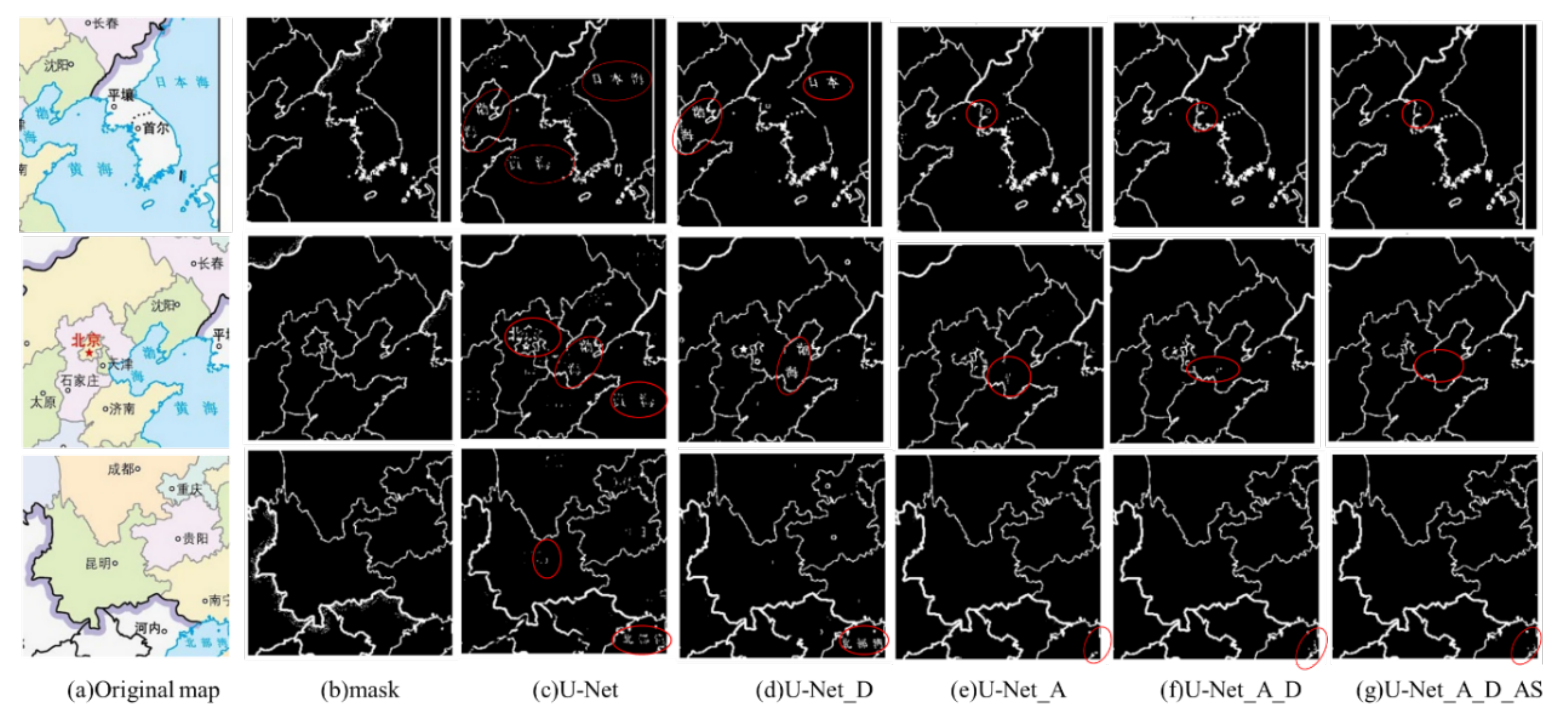The U-Net network is the classic encoder and decoder network, and there are many improved networks based on it, such as U-Net ++ [24] and U-Net +++, which can realize the convolution operation of images of any size and obtain the contextual information of the image through the maximum pooling sampling to reduce the amount of computation [25]. However, due to the repeated use of pooling operations in U-Net, the resolution of feature maps is reduced, leading to rough predicted results. Using down-sampling operations to extract abstract semantic information as features will lead to the loss of some detailed semantic information, causing the problem of missing details and semantic ambiguity in the extracted results. When the U-Net model is directly used to extract line features of the raster map, there will be text interference and broken lines. Therefore, it is necessary to combine other network modules to improve the performance.

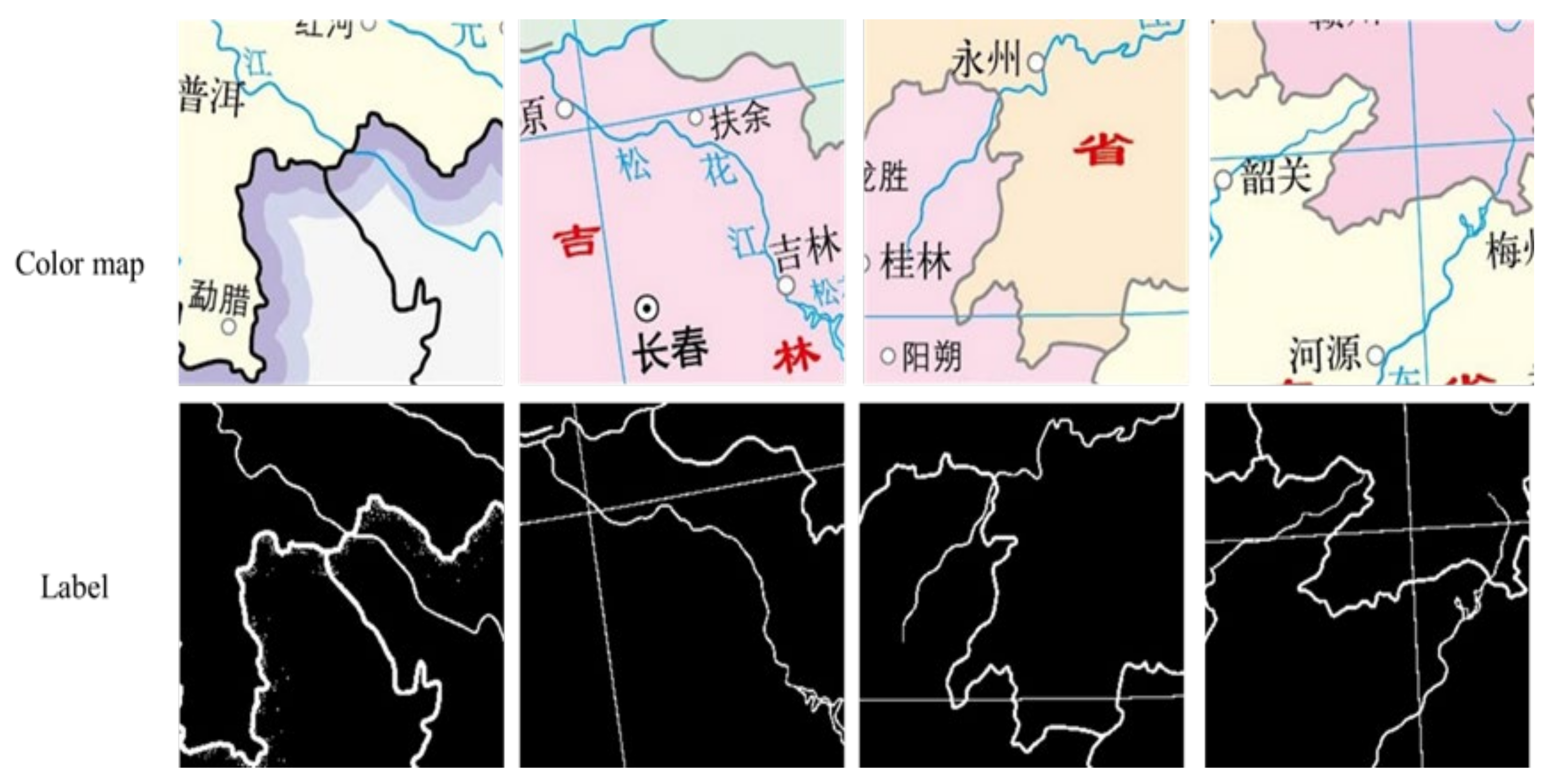
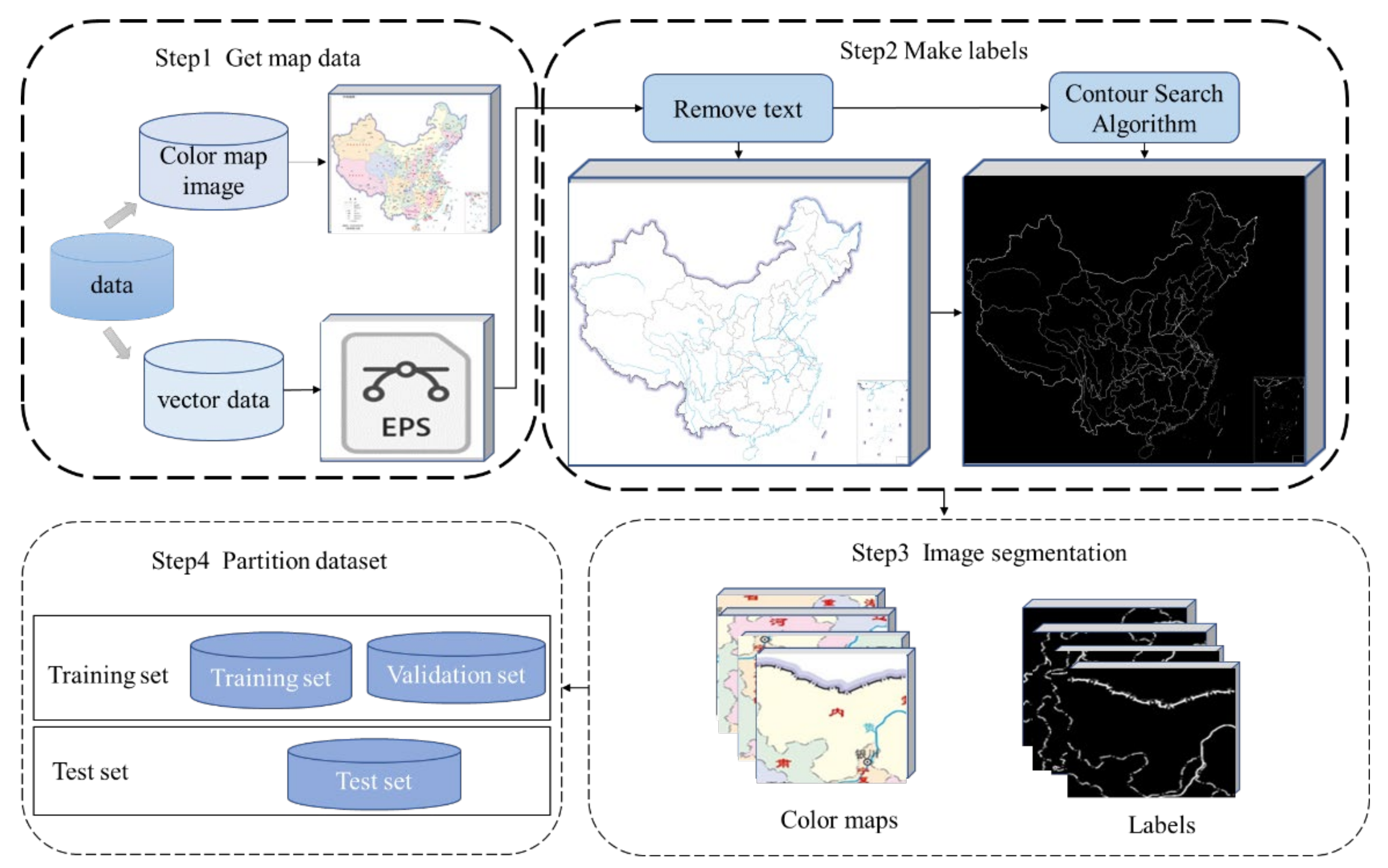
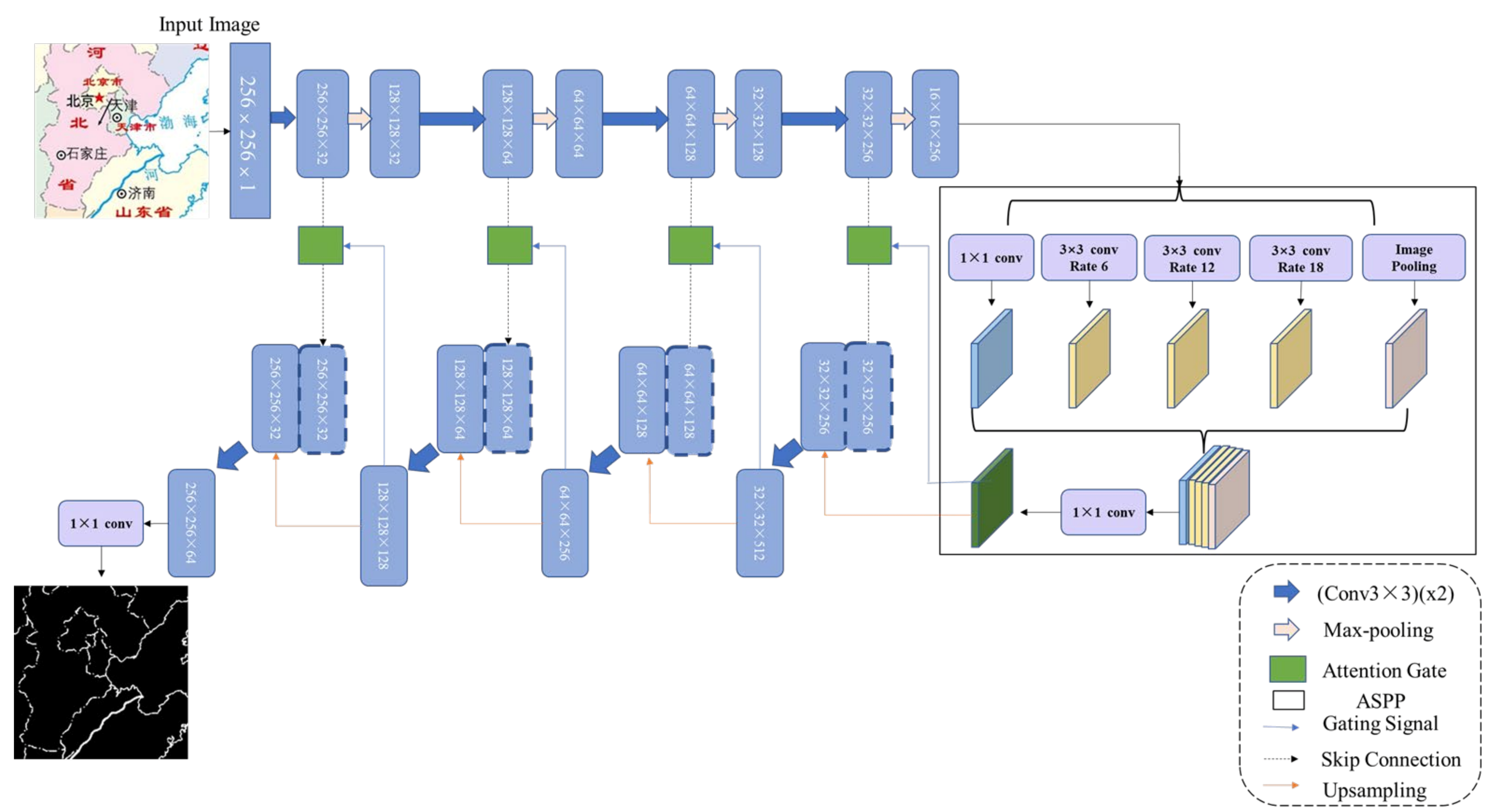
To solve the problems existing in line feature extraction of scanned maps, we constructed test and training datasets based on a raster map. Based on the original U-Net network model, the AG and ASPP modules were added, and an improved U-Net deep network model was proposed to realize the automatic extraction of raster map line features.

2. Data and Methods

2.1. Building the Sample Dataset

Since there is no public dataset of line feature extraction from map images, we constructed a line feature extraction sample set. It mainly includes four processes: acquiring map data, making labels, image segmentation, and dataset division (Figure 1).

2.1.1. Acquiring Map Data

The map data were downloaded from the Chinese Standard Map Service website (http://bzdt.ch.mnr.gov.cn/ (accessed on 25 July 2022)). This web page provides standard maps in JPG and EPS format. JPG is the raster image and EPS is the vector image, which provides favorable conditions for generating label files quickly and accurately. Seven maps with different scales and different areas were collected. The raster images are the images for line feature extraction, and the vector images are used to make the corresponding label files. Detailed attributes of the collected maps are shown in

Table 1. Dataset details.

Map	Width (Pixel)	Height (Pixel)	Resolution (dpi)	Bit Depth	Scale (Million)
A	2127	1628	300	24	1:32
B	5774	4218	300	24	1:7
C	3579	5021	300	24	1:2.1
B	2184	2622	300	24	1:30
E	4208	3178	300	24	1:16
F	1105	1348	300	24	1:60
G	8954	6413	300	24	1:11

.

2.1.2. Making Labels

A map in EPS format contains the interference elements, such as notes, point marks, etc. Through vector data editing software, interference elements in each vector map are deleted, and only line features are retained, and then saved as image data in JPG format. Finally, the line features of JPG format image data are binarized to make label files. The pixel value of the line feature is set to 255, and the pixel value of the background is set to 0. Then, the binary images are used as label data for network training.

2.1.3. Image Segmentation

An entire map could not be fed directly to the input of the proposed network model. Therefore, the size of the training images was reduced to 256 × 256. The sliding window was used to cut out the origin image. The sliding window size was set to 256 × 256, and the position of the sliding window on the image was randomly generated to crop the image. Finally, 1400 images with a size of 256 × 256 were obtained. To speed up the convergence of the network, the images were normalized before being input into the network. To avoid the interference of images of non-line features in network training, the small block images of non-line features were deleted to obtain 1190 image sample datasets.

2.1.4. Dataset Division

The images were divided into a training set and a validation set in a 7:3 ratio. Among them, 883 images were used for training, and 357 images were used for validation.

Figure 1. Training set construction process.

Figure 1. Training set construction process.

Figure 2 shows an example of the sample dataset. The whole color map is cropped into 256 × 256 images, and the corresponding label data are also cropped into 256 × 256 images.

2.2. Improved U-Net Model

2.2.1. Improved U-Net Model Architecture

Based on the classic U-Net network as the basic framework, we designed a more conducive network model for the extraction of map line features. The improved U-Net network structure is shown in Figure 3. U-Net is a network architecture composed of a full convolution, used to perform semantic segmentation tasks. The network structure is symmetric, with an encoder to extract spatial features from images and a decoder to construct segmentation maps from coding features.

The encoder follows the structure of a typical convolutional network. It contains a total of four blocks. Each block in the contracting path consists of two successive 3 × 3 convolutions, followed by a ReLU activation unit and a max pooling layer. Considering the influence of the ReLU activation function on the distribution of output data, the initialization mode of the convolution kernel is set as a normal He initialization, he_normal. It takes samples from truncated normal distribution, as shown in Equation (1), with standard deviation so that the variance of the input and output data is consistent. To keep the size of the feature graph obtained after convolution unchanged, the filling method of the feature graph is set as padding. After the convolution operation, a neuron random inactivation (dropout) layer is added after the convolution layer to avoid overfitting. That is, a certain proportion of convolution kernels in the previous layer are randomly inactivated so that they cannot participate in feature extraction in this round of training, and the parameters of these convolution sums are not updated. The ratio of random inactivation of neurons set in this paper is 0.2. Then, there is a maximum pooling operation with a pool size of 2 × 2 and a step of two. This sequence is repeated four times, and in each down-sampling process, the number of filters in the convolution layer is doubled, amounting to 32, 64, 128, and 256, respectively.

$$\mathrm{std}=sqrt(2/fan\_in)$$

(1)

here, std stands for the standard deviation and $fan\_in$ refers to the number of input units in the weight tensor.

Between the encoder and the decoder, the ASPP module is used to connect them. In the ASPP module, the dilated convolution with sampling levels of 1, 2, 4, and 8 is used for convolution calculation of input features, so that the size of the receptive field is 3, 7, 15, and 31, respectively. New feature maps are obtained by fusing feature maps of different sampling levels. The ASPP module is described in detail in a later section.

The decoder and the encoder belong to a symmetric structure, and the decoder part also contains four blocks. Each block up-samples the feature map using 3 × 3 up-convolution, and the number of filters in the convolution layer is 256, 128, 64, and 32. Then, the feature map from the corresponding layer in the contracting path is cropped and concatenated onto the up-sampled feature map. The initialization mode of the convolution kernel is still set as He initialization, and the feature graph is filled with padding. Finally, a 1 × 1 convolution operation is connected to change the channel number of the feature graph into the category number of classification, and Sigmoid is used for the activation function. The AG module is described in detail in the following sections.

2.2.2. The AG Module in the Model

The idea of the AG module is to enhance the learning ability of the convolutional neural network model to line features by increasing the weight of line features of the color map, to suppress the noise of text in the map background and improve the extraction effect of map line features (Figure 4). $x_i^l$ represents the feature graph obtained by the encoder module, and $g_i^{}$ represents the feature graph obtained by the decoder module through up-sampling. Xi is convolved with 1 × 1 to obtain the weight $W_x^{}$, and $g_i^{}$ is convolved with 1 × 1 to obtain the weight $W_g$, and then they are added together. $q_{attn}^l$ is obtained by using the ReLU activation function and convolution function, ψ, for a 1 × 1 × 1 convolution operation, and then the final attention coefficient $q_{attn}^l$ is obtained by using the activation function Sigmoid for $q_{attn}^l$. Finally, the attention coefficient obtained is multiplied by the input feature $x_i^l$ to obtain the final output feature ${\widehat{x}}_{i,c}^l$. The calculation formulas of the attention coefficient of the attention mechanism in the AG module are Equations (2) and (3), respectively:

$$q_{attn}^l=\mathrm{\Psi }[{\sigma }_1(W_x^T{x}_i^l+W_g^T{g}_i^{}+b_g)]+b_{\mathrm{\Psi }},$$

(2)

$${\alpha }_i^l={\sigma }_2(q_{attn}^l),$$

(3)

where $\mathrm{\Psi }$ represents the convolution function of size 1 × 1 × 1, ${\sigma }_1$ represents the ReLU activation function, $W_x^{}$ is the corresponding weight value of input feature $x_i^l$, $x_i^l$ is the input feature, $W_g$ is the weight value corresponding to the selected communication number $g_i$, $g_i$ is the optional communication number, $b_g$ is the offset value of the selected communication signal, $b_{\mathrm{\Psi }}$ is the bias value corresponding to the convolution function of 1 × 1 × 1, and ${\sigma }_2$ is the Sigmoid activation function.

2.2.3. The ASPP Module in the Model

The latest ASPP module was proposed by Chen et al. [26]. It integrates multi-scale information into ASPP through parallel multiple cavities’ convolution with different proportions to obtain fine segmentation results. The ASPP module has better detection performance for map line features with different scale shapes.

Aiming at the extraction of slender map line features, the ASPP module is added to the last layer of the encoder. The ASPP module adds voids to the general convolution kernel, and the voids of different levels of convolution kernels realize the increase in the receptive field without increasing the computational load (Figure 5). The calculation method of dilated convolution is shown in Equation (4). In this structure, different sampling layers in the coding layer are used as input, and the output of the corresponding upper sampling layer is summed up as the input of the next upper sampling layer. The dilated convolution structure uses the dilated convolution with the sampling levels of 1, 2, 4, and 8 to carry out convolution operation on the input feature graph, so the receptive field size of each layer is 3, 7, 15, and 31, respectively. Feature maps of different sampling levels are used for the model calculation to obtain different scale features, and finally, the fusion between features is carried out. Multi-scale spatial information of feature maps is fully extracted and used to adapt to line feature extraction of the map.

$$y[i,j]={\displaystyle \sum _{k=1}^{k}x[i+r\ast k,j+r\ast k]\omega [k]},$$

(4)

here, $y[i,j]$ is the output of the dilated convolution, $x[i,j]$ is the input, $\omega [k]$ is the convolution kernel of size k, and r represents different sampling levels of the convolution kernel.

2.3. Network Parameter Design

The loss function, optimizer, and learning rate settings used in the improved network are as follows.

2.3.1. Loss Function

Dice loss [27,28] was selected as the loss function. The Dice coefficient is a function of set similarity measurement, usually used to calculate the similarity of two samples, and its value ranges from 0 to 1. The calculation formula of Dice loss is shown in Equation (5):

$$\mathrm{Loss}=1-\frac{2|X\cap Y|}{\left|X\right|+\left|Y\right|},$$

(5)

here, $\left|X\cap Y\right|$ represents the intersection between $X$ and $Y$, and $\left|X\right|$ and $\left|Y\right|$ represent the number of pixels in the predicted label $X$ and the ground truth $Y$, respectively.

2.3.2. Optimizer

We selected the Adam optimizer in the neural network training. Compared with other optimizers, the Adam optimizer has significant advantages [29]; for example, parameter update is not affected by gradient scaling transformation. Moreover, the Adam optimizer has efficient computing and fewer memory requirements, the updated step size can be limited to a rough range, etc.

2.3.3. Learning Rate

The learning rate is the hyperparameter of network weight adjusted by the gradient of the loss function. The initial learning rate is set to 0.001, and the loss platform is set. Training ten times per iteration, if the loss rate does not change much, the learning rate will decrease. The decrease in the learning rate is shown in Equation (6), and the minimum value that the learning rate can decrease to is set as 0.000001. We setup the early stop mechanism to avoid network overfitting during training.

$$lr=l{r}_0\times 0.1$$

(6)

here, $lr$ represents the learning rate, and $l{r}_0$ represents the initial learning rate.

2.4. Model Validation Method

To evaluate the results more comprehensively, we adopted both regional and classification accuracy evaluation indices [30,31]. The selected evaluation indices include the Dice similarity coefficient (DSC), precision, recall, and F1-score.

The Dice coefficient is a region-based evaluation index, focusing on the overlap between the label reference region and automatic segmentation results in the spatial dimension. DSC evaluation experiment results are pixel-level evaluations. The real line feature appears in area A, and the line feature predicted by the network model appears in area B. The Dice coefficient formula is Equation (7):

$$Dice=\frac{2|A\cap B|}{A+B}$$

(7)

The extraction of map line features is a dichotomous problem. Precision, recall, and F1-score are the evaluation indexes based on pixel classification, focusing on the coincidence degree between the label reference area and the contour of the automatic segmentation result. The line feature information is a positive sample, and the background information is a negative sample. All the prediction results can be divided into four categories: the true positive (TP) represents the number of pixels of elements on the correct classification line, the true negative (TN) represents the number of background pixels that are correctly classified, the false positive (FP) represents the number of background pixels that are mistakenly divided into line features, and the false negative (FN) represents the number of line feature pixels mistakenly classified as background pixels. According to these indicators, the calculation formulas for precision, recall, and F1-score are Equations (8)–(10), respectively.

$$Precision=\frac{TP}{TP+FP}$$

(8)

$$\mathrm{Re}call=\frac{TP}{TP+FN}$$

(9)

$$F1=\frac{2\times \mathrm{Precision}\times \mathrm{Recall}}{\mathrm{Precision}+\mathrm{Recall}}$$

(10)

3. Experimental Results and Analysis

This experiment was run in a Linux system environment. The running framework was Tensorflow2.5, and GPU acceleration was used. The server processor was Intel(R) Core (TM) (Intel Corporation, Santa Clara, CA, USA) i9-10980XE GPU @ 3.00 GHz, and the graphics card was NVIDIA GeForce GTX 3080(Santa Clara, CA, USA). The programming environment was Python 3.8.8(Guido van Rossum, The Netherlands).

Table 2. Parameter settings.

Experimental Data	Number	Experimental Environment Parameters
		Frame	TensorFlow
Training set	833	Initial learning rate	0.01
Validation set	357	Optimizer	Adam
Test set	50	Batch size	10

shows the experiment’s parameter settings.

3.1. Influence of Different Network Depths on Extraction Results

Different network depths were selected to analyze their influence on map line feature extraction.

Table 3. Network parameters at different depths.

Network Depth (MB)	Total Parameters (MB)	Trainable Parameters (MB)	Nontrainable Parameters (MB)
4	2.8247	2.8243	0.00037
6	3.8966	3.8957	0.00085
8	7.3685	7.3667	0.00183

shows the number of network parameters when the network depth is 4, 6, and 8. As can be seen from Table 3, as the number of network layers deepens, the number of network parameters increases at double the speed.

Table 4. DSC, precision, and recall rates of networks with different depths.

	Validation Set			Test Set
Network Depth	DSC (%)	Precision (%)	Recall (%)	DSC (%)	Precision (%)	Recall (%)
4	89.37	91.51	87.14	91.73	93.96	89.57
6	90.44	93.23	88.87	92.67	95.08	90.43
8	92.07	95.28	89.12	94.05	95.86	92.34

shows the accuracy evaluation results after experiments with different network depths. It can be seen that with the increase in network depth, the values of DSC, precision, and recall in the test set reached the optimal values, which were 94.05%, 95.86%, and 92.34%, respectively. Although the number of network parameters at layer 8 is larger than that at layers 4 and 6, the increase in parameters can be ignored compared with the accuracy of its extraction.

Figure 6 shows the comparison of map line feature extraction results of different networks. The red boxes in the figure indicate the obvious differences. As can be seen from the figure, when the network depth is 4, the interference of text information in the extraction results is more serious, the extraction effect of map line features details is not favorable, and there is noise interference. When the network depth is 6, the extraction result is better than when the network depth is 4, but there still exists the interference of text. When the network depth is 8, there is almost no text interference in the network, and the details of online feature extraction are also better. The results show that with the deepening of the network, the text interference gradually decreases, and the extracted lines become more and more complete.

When the network depth is 8, the line feature extraction has reached the ideal effect; therefore, we selected 8 layers for the final network depth.

3.2. Influence of Different Addition Modules on Extraction Results

By adding different modules, the influence of the network on the line feature extraction was tested. The experimental results are shown in

Table 5. DSC, precision, recall, and F1-score of different basic networks.

Network	DSC (%)	Precision (%)	Recall (%)	F1 (%)
U_Net	85.93	86.69	84.13	85.39
U_Net_D	91.18	91.73	90.70	91.21
U_Net_A	92.66	94.88	91.80	93.31
U_Net_A_D	92.57	93.22	91.99	92.60
U_Net_A_D_AS	93.03	93.08	92.29	92.68

Bold is the optimal value for each column.

, where U_Net_D represents adding a random inactivation layer after the convolution layer. U_Net_A represents the network added to the attention mechanism module, U_Net_A_D represents the network in which the random inactivation layer of neurons and the attentional mechanism module are added simultaneously, and U_Net_A_D_AS represents the network in which the random inactivation layer of neurons and the ASPP module are added simultaneously. It can be seen from Table 5 that compared with the original U-Net network, the network integrating the attention mechanism and ASPP module improved the DSC by 7.10%, the precision by 6.39%, the recall by 8.16%, and the F1-score by 7.29% in the test set. When only the attention mechanism module was added to the network, the precision reached the highest value of 94.88%, but the DSC was not as high as that when adding the attention mechanism and the ASPP module at the same time. When the attention and ASPP module were added at the same time, the DSC and the recall reached the highest values of 93.03% and 92.29%, respectively.

The learning curve of the training in the experiment is shown in Figure 7. In the figure, the red curve is the loss curve of the training set, and the blue curve is the loss curve of the verification set. The horizontal axis is the number of training iterations, and the vertical axis is the loss value. In the experiment, the total number of training times was 100, because the number of datasets was relatively small, and the network model was relatively simple. As can be seen from the learning curve of the training set, the final trend of the loss curve in the improved U-Net model proposed in this paper tended to be stable, and the accuracy was significantly improved compared with other networks.

The map line feature extraction results after adding different modules are shown in Figure 8. As can be seen from the resulting figure, the extracted line features also contain certain text information, marked with red circles in the figure. Figure 8g is the extraction result of the model proposed in this paper. It can be seen from the resulting figure that the influence of characters has been greatly improved.

3.3. Test of Map Images with Different Language Characters

We use the trained model to test map images annotated as English characters. A total of 99 map images were tested. The experimental results are shown in

Table 6. Test results of English character map.

Network	DSC (%)	Precision (%)	Recall (%)	F1 (%)
U_Net	67.69	58.83	79.95	67.78
U_Net_D	68.28	58.09	82.98	68.34
U_Net_A	71.12	62.28	82.30	70.90
U_Net_A_D	71.08	61.80	83.04	70.86
U_Net_A_D_AS	70.95	62.30	82.56	71.01

. It can be seen from Table 6 that the accuracy will be much lower than that of map images with Chinese characters. We compared the results of the Chinese character map obtained in Table 5 with those of the English character map obtained in Table 6 by selecting the highest evaluation indexes. We found that the DSC decreased by 21.91%, the precision decreased by 32.58%, the recall decreased by 9.25%, and the F1-score decreased by 22.3%. This is because the images in the training set used in the training model are all map images of Chinese characters. However, characters in different languages have different characteristics. Therefore, if the model without English character map training is directly applied to the map image with English characters, its accuracy will considerably decrease.

The extraction results of line features of the English character map are shown in Figure 9. Compared with the original U-Net network, the improved U-Net network also had a better effect when tested with English character map images. It can be seen from the result that the size of English characters has a certain influence on the extraction of map line features. If the English characters in the map are too large, they will be easily confused with the line features of the map.

3.4. Improved U-Net Model Robustness Test

The robustness of the network was tested by adding random noise to the raster map. In the image, the signal-to-noise ratio (SNR) is usually used to measure the image noise. In this paper, the proportion of signal pixels was used as the SNR to measure the amount of added noise. In this paper, the SNRs of 0.01, 0.02, 0.03, 0.04, and 0.05 were selected to test the effect of network extraction of map line features.

Table 7. Comparison of DSC between the improved network and the original network.

SNR	0.01	0.02	0.03	0.04	0.05
U_Net	46.80	42.85	39.64	36.31	32.46
U_Net_D	46.54	39.34	35.43	32.92	32.01
U_Net_A	48.99	42.03	37.35	33.39	30.56
U_Net_A_D	48.26	41.75	36.46	32.06	28.27
Improved U-Net	63.85	57.96	54.05	50.12	47.01

shows the DSC comparison of extraction results of different SNR line features. Compared with the original U-Net network, the improved U-Net network model in this paper has a greatly improved anti-noise ability. When the SNR was 0.01, the DSC of the improved network increased by 17.05%. When the SNR was 0.02, the DSC increased by 15.11%. When the SNR was 0.03, the DSC increased by 14.41%. When the SNR was 0.04, the DSC increased by 13.18%. When the SNR was 0.05, the DSC increased by 14.55%.

Figure 10 shows the line feature extraction results of a sample in the test set. Figure 10a is the label of the selected sample, and Figure 10b–f show the extraction results of map line features of color maps with SNRs of 0.01, 0.02, 0.03, 0.04, and 0.05, with the original U-Net network and improved U-Net network.

The red box in Figure 10 highlights an obvious difference. When the SNR was 0.01, the original U-Net network had broken lines and lost line features, as marked in the red box in the image extracted by U-Net in Figure 10b. However, when the SNR of the improved U-Net network was 0.05, the disconnection occurred, as indicated in the red box in the improved U-Net extraction result in Figure 10f. The original U-Net lost line features more seriously when the SNR was 0.05. It can be seen from the experiment that the improved U-Net network proposed in this paper has better robustness in online feature extraction than the traditional U-Net network.

4. Discussion

Maps store valuable information documenting human activities and natural features on Earth over long periods of time. Understanding how to make full use of the data information in maps has become a difficult point in research. Due to the complexity of map images compared with general images, various elements on maps are interlaced and overlapped, which increases the complexity of map elements’ extraction. Much existing research on maps is aimed at the recognition or detection of symbols on maps [7,9,16,23], such as identifying urban districts, hotels, and architectural markers on a map. The recognition and extraction of map line features are mostly based on traditional algorithms.

There are two major challenges in applying semantic segmentation CNNs to maps for automatically extracting geographic features. The first challenge is generating accurate object boundaries, which is still an open research topic in semantic segmentation. The second challenge is that semantic segmentation models trained with the publicly available labeled datasets do not work well for maps without a sufficient amount of labeled training data from map scans. To fully take advantage of the valuable content in historical map series, advanced semantic segmentation methods that can handle small objects and extract precise boundaries still need to be developed.

The model for extracting geographic line features trained in this paper has certain limitations. Since the dataset used in training the model is relatively simple, there is no adequate generalization for maps with different characters in different countries and languages. To make the model more generalized, it is necessary to enrich the types of map samples in the training set. Overall, the sample size of the current dataset is not large enough to apply the model to more kinds of maps.

5. Conclusions

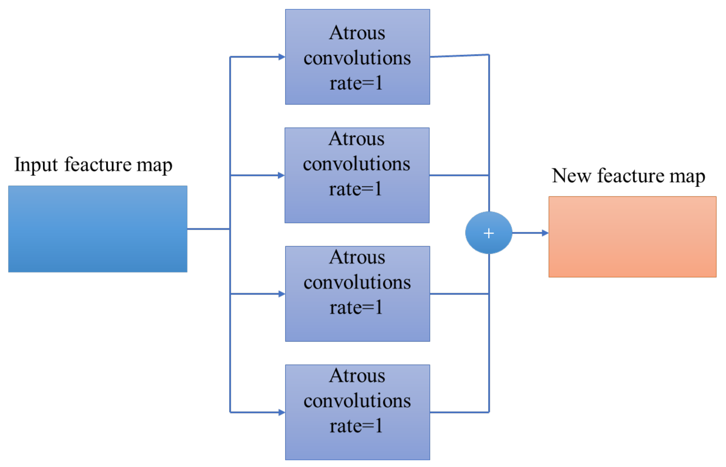
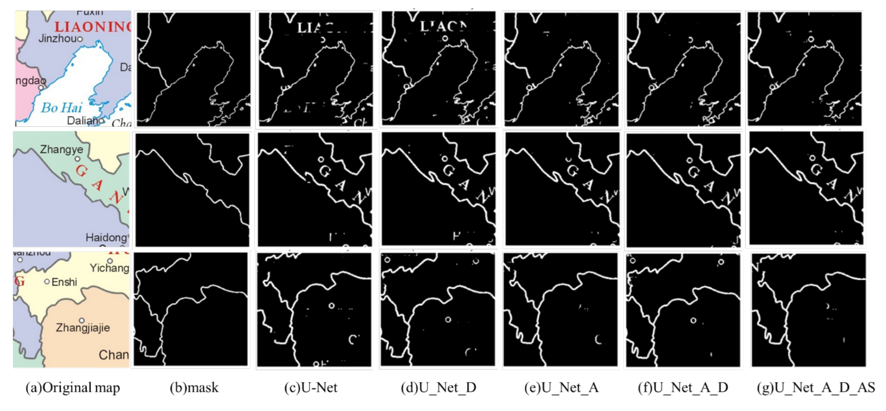
In this paper, we introduced ASPP and AG modules into the traditional U-Net network, constructed the sample set of map line feature extraction, and proposed an improved U-Net network model for scanning map line feature extraction. The AG module increased the weight of line feature extraction and reduced the interference of background text. The ASPP module was used to extract features of different scales to improve the segmentation effect. Through comparative analysis of experiments designed with different network depths, network modules, and robustness testing, our conclusions are as follows:

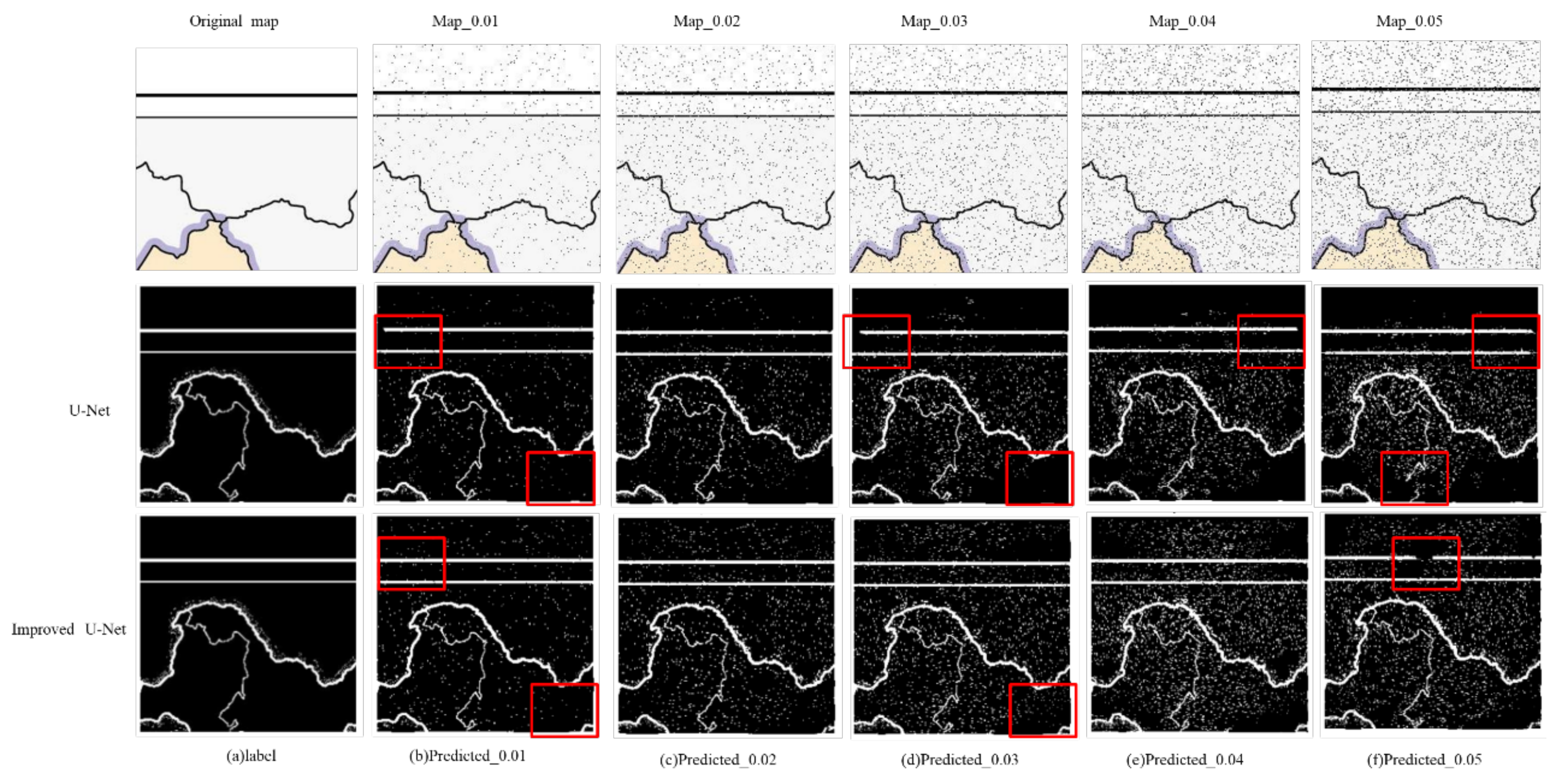
• The improved U-Net network we proposed achieved the accurate automatic extraction of grid map line features, and the DSC accuracy of the extraction results reached 93.3%. Compared with the traditional U-Net network model, the DSC was increased by 7.1%, the accuracy was increased by 6.39%, and the recall rate was increased by 8.16%. In the presence of noise, when the SNR was 0.01, the accuracy of DSC was improved by 17.05%. When the SNR was 0.02, DSC increased by 15.11%. When the SNR was 0.03, DSC increased by 14.41%. When the SNR was 0.04, DSC increased by 13.18%. When the SNR was 0.05, DSC increased by 14.55%.
• The improved U-Net network proposed here had better anti-noise ability and better robustness in raster map line feature extraction than the traditional U-Net network, indicating its superior extensibility.

In this work, we achieved automatic extraction of raster map line features based on the deep learning method. However, due to the limitations of data sources and the heavy workload of manual vectorization of maps, the map styles and types in the sample dataset created in this paper are slightly monotonous. The network model proposed in this paper must be further tested and improved for more line feature extraction sample sets in the future.

References

1. Chiang, Y.Y.; Moghaddam, S.; Gupta, S.; Fernandes, R.; Knoblock, C.A. From map images to geographic names. In Proceedings of the 22nd ACM SIGSPATIAL International Conference on Advances in Geographic Information Systems, Dallas/Fort Worth, TX, USA, 4–7 November 2014; pp. 581–584. [Google Scholar]
2. Yu, R.; Luo, Z.; Chiang, Y.Y. Recognizing text in historical maps using maps from multiple time periods. In Proceedings of the 2016 23rd International Conference on Pattern Recognition (ICPR), Cancún, Mexico, 4–8 December 2016. [Google Scholar]
3. Fletcher, L.A.; Kasturi, R. A robust algorithm for text string separation from mixed text/graphics images. IEEE Trans. Pattern Anal Mach Intell. 1988, 10, 910–918. [Google Scholar] [CrossRef]
4. Zhang, T.; Yin, Y.L.; Liu, X.L. Automatic Recognition of Point-Shaped Symbols in Scanned Maps. Eng. Surv. Mapp. 2000, 3, 15–18. [Google Scholar] [CrossRef]
5. Illert, A. Automatic Digitization of Large-Scale Maps. In Proceedings of the 1991 Acsm-Asprs Annual Convention, Baltimore, MD, USA, 25–29 March 1991; pp. 113–122. [Google Scholar]
6. Ohsawa, Y.; Sakauchi, M.; Murakami, A.; Kamada, K. Automatic Recognition of Road Information on Medium Scale Topographical Maps. Available online: https://www.isprs.org/proceedings/XXVII/congress/part3/350_XXVII-part3-sup.pdf (accessed on 26 July 2022).
7. Satoshi, S.; Makoto, K.; Toshio, H. Errata: Automatic Line Drawing Recognition Of Large-Scale Maps. Opt. Eng. 1987, 26, 826. [Google Scholar]
8. Nagy, G.; Samalz, A.; Sethz, S.; Fisherz, T.; Guthmann, E.; Kalafala, K.; Li, L.; Sivasubramaniam, S.; Xu, Y. Reading Street Names from Maps—Technical Challenges. In Proceedings of the GIS/LIS Conference, Washington, DC, USA, 20 November 1998; pp. 89–97. [Google Scholar]
9. Chiang, Y.Y.; Knoblock, C.A. Recognizing text in raster maps. Geoinformatica 2015, 19, 1–27. [Google Scholar] [CrossRef]
10. Chiang, Y.Y.; Leyk, S.; Nazari, N.H.; Moghaddam, S.; Tan, T.X. Assessing the impact of graphical quality on automatic text recognition in digital maps. Comput. Geosci. 2016, 93, 21–35. [Google Scholar] [CrossRef]
11. Lladós, J.; Valveny, E.; Sánchez, G.; Martí, E. Symbol Recognition: Current Advances and Perspectives. In Proceedings of the 4th International Workshop, GREC 2001, Kingston, ON, Canada, 7–8 September 2001. [Google Scholar]
12. Chiang, Y.-Y.; Leyk, S.; Knoblock, C.A. A Survey of Digital Map Processing Techniques. ACM Comput. Surv. 2014, 47, 1–44. [Google Scholar] [CrossRef]
13. Beattie, C.S. 3D visualization models as a tool for reconstructing the historical landscape of the Ballona Creek watershed. China Fiber Insp. 2011, 99, 290–300. [Google Scholar]
14. Levachkine, S.; Velázquez, A.; Alexandrov, V.; Kharinov, M. Semantic Analysis and Recognition of Raster-Scanned Color Cartographic Images. In International Workshop on Graphics Recognition; Springer: Berlin/Heidelberg, Germany, 2001; pp. 178–189. [Google Scholar]
15. Lim, Y.W.; Sang, U.L. On the color image segmentation algorithm based on the thresholding and the fuzzy c-means techniques. Pattern Recog. 1990, 23, 935–952. [Google Scholar]
16. Du, J.; Zhang, Y. Automatic extraction of contour lines from scanned topographic map. In Proceedings of the IEEE International Geoscience & Remote Sensing Symposium, Anchorage, Alaska, USA, 20–24 September 2004. [Google Scholar]
17. Wang, S.; Zhang, Z.; Wwn, W.; Qiu, Z. Automated Color Segmentation in Maps Based on Theory of Color and Mathematical Morphology. Bull. Surv. Mapp. 2001, 10, 334–340. [Google Scholar]
18. Budig, B. Extracting Spatial Information from Historical Maps: Algorithms and Interaction; BoD–Books on Demand: Hamburg, Germany, 2018. [Google Scholar]
19. Li, W.; Shuai, X.; Liu, J. Segmentation of color contour map based on Matlab. Geospat. Inf. 2021, 19, 80–82+85. [Google Scholar] [CrossRef]
20. LeCun, Y.; Bengio, Y.; Hinton, G. Deep learning. Nature 2015, 521, 436–444. [Google Scholar] [CrossRef] [PubMed]
21. Duan, W.; Chiang, Y.Y.; Knoblock, C.; Jain, V.; Dan, F.; Uhl, J.H.; Leyk, S. Automatic alignment of geographic features in contemporary vector data and historical maps. In Proceedings of the 1st workshop on artificial intelligence and deep learning for geographic knowledge discovery, Los Angeles, CA, USA, 7–10 November 2017; pp. 45–54. [Google Scholar]
22. Uhl, J.H.; Leyk, S.; Chiang, Y.Y.; Duan, W.; Knoblock, C.A. Extracting Human Settlement Footprint from Historical Topographic Map Series Using Context-Based Machine Learning. In Proceedings of the ICPRS 2017, 8th International Conference on Pattern Recognition Systems, Madrid, Spain, 11–13 July 2017. [Google Scholar]
23. Uhl, J.H.; Leyk, S.; Chiang, Y.Y.; Duan, W.; Knoblock, C.A. Spatialising uncertainty in image segmentation using weakly supervised convolutional neural networks: A case study from historical map processing. IET Image Proc. 2018, 12, 2084–2091. [Google Scholar] [CrossRef]
24. Peng, D.F.; Zhang, Y.J.; Guan, H.Y. End-to-End Change Detection for High Resolution Satellite Images Using Improved UNet plus. Remote Sens. 2019, 11, 1382. [Google Scholar] [CrossRef] [Green Version]
25. Ronneberger, O.; Fischer, P.; Brox, T. U-Net: Convolutional Networks for Biomedical Image Segmentation. Med. Image Comput. Comput.-Assist. Interv. Pt Iii 2015, 9351, 234–241. [Google Scholar] [CrossRef] [Green Version]
26. Chen, L.C.E.; Zhu, Y.K.; Papandreou, G.; Schroff, F.; Adam, H. Encoder-Decoder with Atrous Separable Convolution for Semantic Image Segmentation. Lect. Notes Comput. Sci. 2018, 11211, 833–851. [Google Scholar] [CrossRef] [Green Version]
27. Chen, X.; Williams, B.M.; Vallabhaneni, S.R.; Czanner, G.; Zheng, Y. Learning Active Contour Models for Medical Image Segmentation. In Proceedings of the 2019 IEEE/CVF Conference on Computer Vision and Pattern Recognition (CVPR), Long Beach, CA, USA, 15–20 June 2019. [Google Scholar]
28. Bosman, A.S.; Engelbrecht, A.; Helbig, M. Visualising Basins of Attraction for the Cross-Entropy and the Squared Error Neural Network Loss Functions. Neurocomputing 2020, 400, 113136. [Google Scholar] [CrossRef] [Green Version]
29. Kingma, D.; Ba, J. Adam: A Method for Stochastic Optimization. arXiv 2014, arXiv:1412.6980. [Google Scholar]
30. Wei, X.; Zhou, Z. Two Performance Evaluation Methods for Classification Problems Based on ROC Curve. Comput. Technol. Dev. 2010, 20, 47–50. [Google Scholar]
31. Wu, B.; Lin, S.; Zhou, G. Quantitatively Evaluating Indexes for Object-based Segmentation of High Spatial Resolution Image. J. Geo-Inform. Sci. 2013, 15, 567–573. [Google Scholar] [CrossRef]
Figure 2. The map dataset.
Ijgi 11 00439 g002
Figure 3. The structure of the improved U-Net model.
Ijgi 11 00439 g003
Figure 4. Schematic diagram of AG module implementation.
Ijgi 11 00439 g004
Figure 5. Schematic diagram of obtaining features of different scales.
Ijgi 11 00439 g005
Figure 6. The network extraction results of different depths: (a) cropped color map image blocks, (b) labels of map line features produced, (c) the result of the network depth is 4, (d) the result of the network depth is 6, and (e) the result of the network depth is 8.
Ijgi 11 00439 g006
Figure 7. Learning curve of network training with different modules: (a) the learning curve of U-Net, (b) the learning curve of U_Net_D, (c) the learning curve of U_Net_A, (d) the learning curve of U_Net_A_D, and (e) the learning curve of U_Net_A_D_AS.
Ijgi 11 00439 g007
Figure 8. The extraction results of line features: (a) cropped color map image blocks, (b) labels of map line features, (c) the U-Net result, (d) the U_Net_D result, (e) the U_Net_A result, (f) the U_Net_A_D result, and (g) the U_Net_A_D_AS result.
Ijgi 11 00439 g008
Figure 9. Extraction results of English character map: (a) cropped color map image blocks, (b) labels of map line features, (c) the U-Net result, (d) the U_Net_D result, (e) the U_Net_A result, (f) the U_Net_A_D result, and (g) the U_Net_A_D_AS result.
Ijgi 11 00439 g009
Figure 10. Experimental results with different SNRs: (a) map line feature labels, (b) the results with SNR of 0.01, (c) the results with SNR of 0.02, (d) the results with SNR of 0.03, (e) the results with SNR of 0.04, and (f) the results with SNR of 0.05.
Ijgi 11 00439 g010