Effects of Climate Change on Corn Yields: Spatiotemporal Evidence from Geographically and Temporally Weighted Regression Model

Abstract

Food security has been one of the greatest global concerns facing the current complicated situation. Among these, the impact of climate change on agricultural production is dynamic over time and space, making it a major challenge to food security. Taking the U.S. Corn Belt as an example, we introduce a geographically and temporally weighted regression (GTWR) model that can handle both temporal and spatial non-stationarity in the relationship between corn yield and meteorological variables. With a high fitting performance (adjusted R² at 0.79), the GTWR model generates spatiotemporally varying coefficients to effectively capture the spatiotemporal heterogeneity without requiring completion of the unbalanced data. This model makes it possible to retain original data to the maximum possible extent and to estimate the results more reliably and realistically. Our regression results showed that climate change had a positive effect on corn yield over the past 40 years, from 1981 to 2020, with temperature having a stronger effect than precipitation. Furthermore, a fuzzy c-means algorithm was used to cluster regions based on spatiotemporally changing trends. We found that the production potential of regions at high latitudes was higher than that of regions at low latitudes, suggesting that the center of productive regions may migrate northward in the future.

1. Introduction

Global food security is a major challenge to the sustainable development goals and implementation of the 2030 Paris Agreement on Climate Change. Climate solutions aiming at effective adaption to climate change are needed, along with further research into its dual role in requiring a response from agri-producers and as a natural factor in food security. In addition to socioeconomic factors such as scientific and technological progress, farming costs and benefits, and land use patterns, these natural factors including soil quality and climatic conditions [1,2,3] are essential to crop production. Beginning in the 1950s, as the scientific evidence of human greenhouse gas emissions affecting important agricultural factors such as temperature and precipitation has continued to accumulate, scholars and experts have become convinced that climate change will significantly impact crop yields [4,5,6,7,8]. Therefore, measuring the potential impact of meteorological variability on crop yield is critical for farm management and food security [9,10].

Many studies have been conducted to understand the impact of climate change on crop yield. For example, using regression analysis of historical data to link past yields with weather realizations, Lobell showed that at national and regional scales temperature changes were more important than precipitation changes for maize, rice, and wheat [11]. Scholars have found that climate extremes have a much stronger impact on crop yield in rain-fed areas than in irrigated areas [12]. In addition, under different conditions, meteorological factors such as precipitation have been shown to have different effects on corn yield [13]. Several studies have shown that the degree of negative susceptibility to excessive precipitation and of positive susceptibility to precipitation under drought conditions are of similar magnitude [14].

In order to research the effects of climate change on crop yield, two modeling strategies have been extensively applied, namely, crop simulation [13,15] and statistical models [2,16,17]. The crop simulation model, known as the process-based model, can accurately control for all crop growth factors (i.e., temperature, humidity, soil, fertilizer, etc.) and examine the impact of different climate change scenarios on crop growth, development, and yield [18]. The decision support system for agrotechnology transfer (DSSAT), for example, typically requires various input data such as crop variety, soil conditions, and farm management [19]. However, crop growth simulation experiments are difficult to implement at large scales, which is necessary in order to obtain professional technical information and can additionally incur high acquisition costs [11]. The second approach is statistical modeling, which extends crop production variables in order to perform regression estimations.

Initially, scholars can estimate the impact of weather by analyzing year-to-year weather changes and their impact on yield using time series models [2,20]. However, considering the long-term impact of climate change on yield changes, as production processes are updated (as exemplified by variety improvement), time-invariant analysis cannot adequately capture the impact [11]. In addition, cross-sectional models that account for spatial autocorrelation have reflected the historical effectiveness of adaptation in maintaining the yield of a crop across different climates.

Next, in light of the heterogeneity of crop production systems and significant inter-annual meteorological variability, the regression coefficients of meteorological variables are expected to vary both spatially and temporally [6,16,21,22,23]. As a result, panel models that consider both time and space have been widely used [24,25,26]. In the past, panel data have allowed for the use of either fixed or random effects models to control for unobserved heterogeneity. Here, we have improved the estimation efficiency by conducting panel data analysis.

However, the panel model has a fatal drawback in that it requires balanced input data and does not perform well with unbalanced data. Therefore, data completion has become a necessary process for research. The most commonly used data completion methods consider similar yield data over similar times or spaces and preset the distribution characteristics of yield in advance. This likely produces interference when determining the relationships between crop outcomes and various climatic factors.

To use original unbalanced data directly and estimate the results more reliably and realistically, we must develop a novel model. At the same time, this new model should deal with both spatial and temporal non-stationary processes. Luckily, a frequently used cross-section model, geographically weighted regression (GWR), has demonstrated a powerful ability to capture related spatial datasets [27,28,29]. Here, we further propose a spatiotemporal regressive model, the geographically and temporally weighted regression (GTWR) model, which provides a broader and more flexible inference basis for spatiotemporal yield variability analysis by accounting for the fusion of temporal and spatial heterogeneity [30]. Meanwhile, using local regression, GTWR can deal effectively with unbalanced data. GTWR has already been widely used to determine spatiotemporal relationships in areas such as housing prices and marine ecology [31,32,33]. Thus, we can use the GTWR model to handle both the unbalanced data and the spatiotemporal non-stationary characteristics of the coefficients.

The purpose of the present research was to reveal persuasive spatial and temporal relationships between meteorological variables and corn yield using county-level data in the U.S. Corn Belt from 1981 to 2020. In order to demonstrate the advantages of this model, we further compared it with ordinary least squares (OLS) (Equation S1) [6], time-linear regression (time-LR, a time series method) (Equation S2) [34], and GWR (a cross-sectional method) (Equation S3) [27] in terms of model fitting performance (Table S1).

The rest of the paper is structured as follows. We introduce the study area and data sources in Section 2. In Section 3, we describe in detail the analytical methods used and propose a set of methods for investigating variation in corn yield with meteorological variables based on the GTWR model. In Section 4, we analyze how climatic variables affect yield changes in time and space. Finally, in Section 5 we summarize our findings, provide conclusions, and discuss the strengths and limitations of the study.

2. Study Area and Data

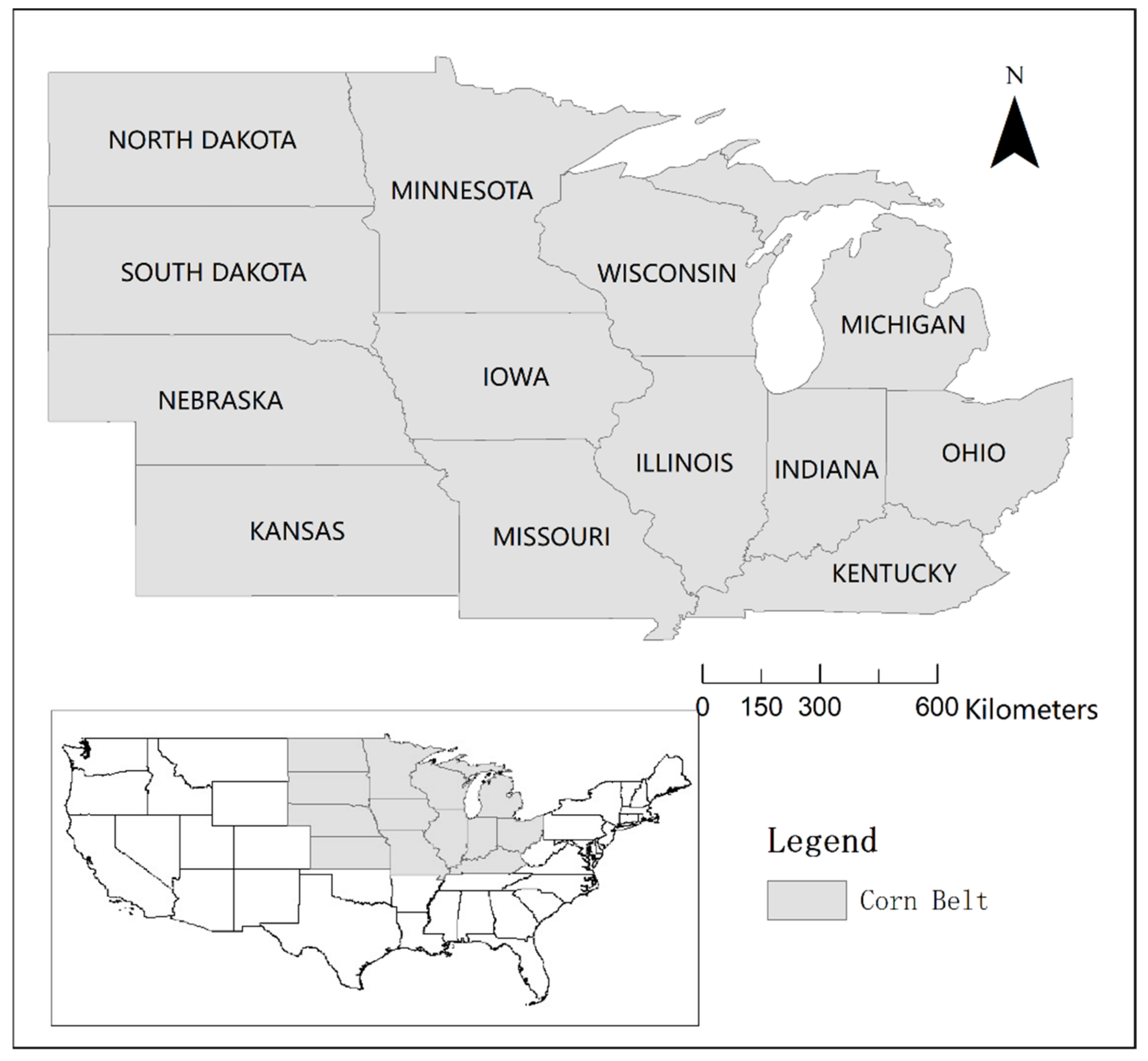
2.1. Study Area

In this study, we focused on the main corn cropping regions in the U.S. (Figure 1). This region, called the Corn Belt, covers 13 States (Illinois, Indiana, Iowa, Kansas, Kentucky, Michigan, Minnesota, Missouri, Nebraska, Ohio, Wisconsin, North Dakota, and South Dakota), and has a humid continental climate with rich and deep soils and is located in the center of the country [35,36]. The Corn Belt is the world’s largest specialized corn-producing area, and has the highest yield [20]; corn production here accounts for three-quarters of the country’s total.

2.2. Data Collection and Preprocessing

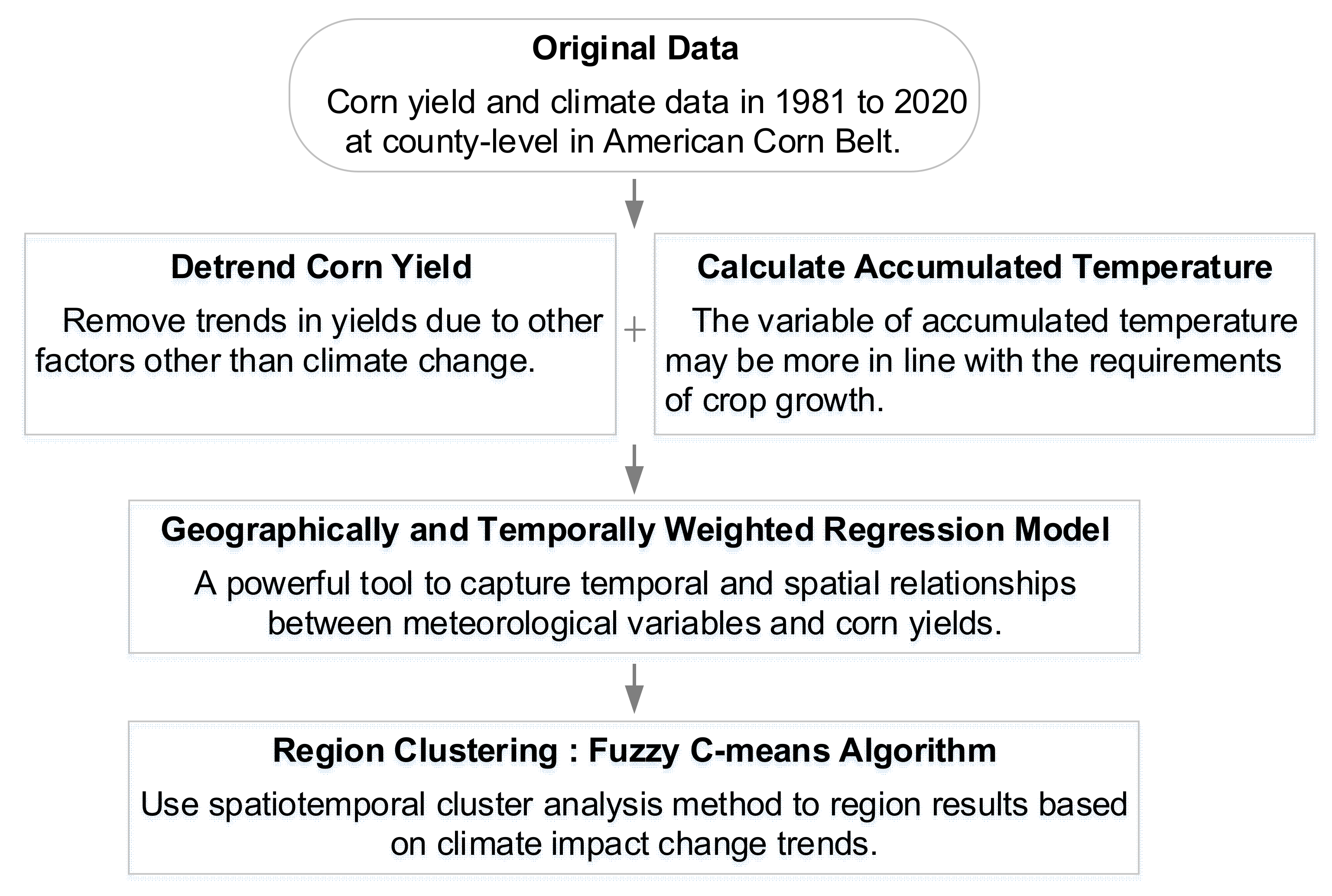
Corn yield data from 1981 to 2020 were collected from the National Agricultural Statistics Service (NASS) of the U.S. Department of Agriculture (USDA) (https://www.nass.usda.gov/, accessed on 24 March 2021) at the county level (unit: tons/acre) and converted to tons/ha. Counties that had too much missing data or no longer grew corn were eliminated.

From the existing data, yield records were occasionally missing for a variety of reasons, making the original yield data unbalanced. For example, certain counties skipped the survey for many years. Fortunately, the method used in this study could handle unbalanced data well, and the preprocessing method no longer completed missing data. Our final sample included 1159 counties and 41,693 county-year records (

Table 1. Corn yield data at the county level (1981–2020).

State Name	County Count	Records
ILLINOIS	102	3965
INDIANA	92	3517
IOWA	99	3931
KANSAS	105	3737
KENTUCKY	113	3775
MICHIGAN	81	2603
MINNESOTA	85	3077
MISSOURI	114	3597
NEBRASKA	93	3524
OHIO	86	3320
WISCONSIN	71	2565
NORTH DAKOTA	53	1747
SOUTH DAKOTA	65	2335
Total	1159	41,693

).

Daily county-level meteorological data were obtained from Parameter Elevation Regression on Independent Slopes (PRISM) (https://prism.oregonstate.edu, accessed on 1 August 2021) using the Applied Climate Information System API (2017). The PRISM variables used for analysis were daily mean air temperature (TEMP), maximum air temperature (T_max), minimum air temperature (T_min), total precipitation (PCPN), maximum vapor pressure deficit (VPD_max), and minimum vapor pressure deficit (VPD_min) [37], all in metric units (°C, mm, hPa).

As PRISM meteorology data are available as continuous surfaces (spatial raster layers) with a spatial resolution of 4 km, zonal statistics were obtained by overlapping the data with county boundaries to estimate the average values of climate-related factors at the county level [6].

3. Methodology

We proposed a novel spatiotemporal analytical framework to measure the potential impact of meteorological variability on crop yield in the U.S. Corn Belt (as shown in Figure 2). First, we needed to remove the portion affected by the time trend from the corn yield data, for which we used the linear detrend method. This enabled us to focus only on climate data. The original climate variables were obtained with new variables that were more in line with the requirements of crop production, such as effective accumulated temperature. A powerful spatiotemporal regression model, the GTWR model, was then implemented to discover the relationships between climate change and crop production by deriving spatiotemporal coefficients. Furthermore, the spatiotemporal coefficients were clustered using a fuzzy c-means algorithm to discover regions with similar trends over the past 40 years.

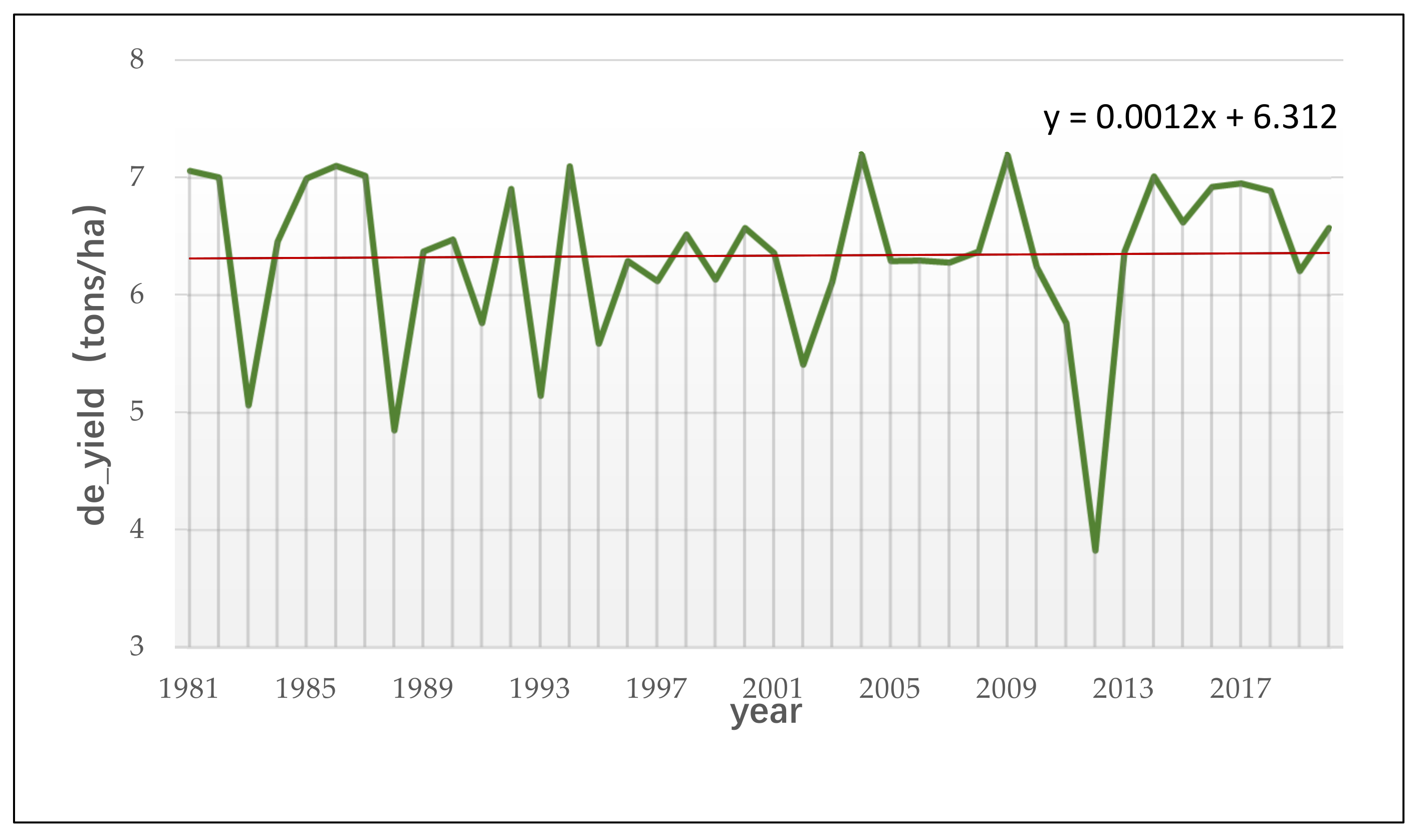
3.1. Linear Detrend Preprocessing

In order to remove the influence of crop growing practices and conditions [38,39], we detrended the corn yield for county $i$ at year $t$ by removing the linear fits for the yield model using Equation (1):

$$Y{d}_{i,t}=Y_{i,t}-Y_{i,t}^{\ast }+Y_{i,1981}^{\ast }$$

(1)

where $Y{d}_{i,t}$ represents the detrended values, $Y_{i,t}$ represents the observed yield, and $Y_{i,t }^{\ast }$ represents the predicted yield; $Y_{i,1981}^{\ast }$ indicates the initial value in the year 1981.

3.2. Interval Accumulated Temperature Method

Generally, the accumulated temperature in a certain temperature range is defined as the effective accumulated temperature and is referred to as growing degree days (GDD) [35,40]. GDD serves as a necessary thermal resource for crop growth. In an extreme temperature range, the accumulated temperature is defined as harmful accumulated temperature, known as killing degree days (KDD) [6,41]; this directly indicates the heat stress. The daily accumulated temperature is summed based on the crop growth period to measure the impact of temperature on crop yield. These two variables can be calculated using Equations (2)–(4):

$$TEMP=\left(Tmax+Tmin\right)/2$$

(2)

$$GDD={{\displaystyle \sum }}_{period}TEMP-Tb$$

(3)

$$KDD={{\displaystyle \sum }}_{period}Tmax-Tu$$

(4)

where $Tu$ and $Tb$, the upper and lower bounds, respectively, are set as 29 °C and 8 °C, respectively [6,42].

3.3. GTWR Model

To fit the inherent spatial non-stationarity of geographic relationships, we harness the idea of local smoothing, specifically a GWR model, to change the regression coefficients alongside changes in spatial location [43,44]. The GWR model is an extension of the OLS model, which embeds the spatial relationship changes caused by spatial position differentiation into the calculation of regression coefficients.

Huang introduced time and space factors to balance the differences in time and space scales, embedded the changes in the time dimension into the GWR model, proposed a method for constructing time and space distance, and established a time and space GTWR model [30]. This derivation proves the theoretical feasibility of replacing time and space factors with space-time factors, thereby reducing computational complexity. Combined with the relationship between crop yield and climate factors studied in this article, the mathematical expression of the GTWR model is described by Equation (5):

$$\begin{array}{cc}d{Y}_{\left(u_i,v_i,t_i\right)}& ={\beta }_{\left(u_i,v_i,t_i\right),0}+{\beta }_{\left(u_i,v_i,t_i\right),1}GD{D}_{\left(u_i,v_i,t_i\right)}+{\beta }_{\left(u_i,v_i,t_i\right),2}KD{D}_{\left(u_i,v_i,t_i\right)}+\\ & {\beta }_{\left(u_i,v_i,t_i\right),3}VP{D}_{\left(u_i,v_i,t_i\right)}+{\beta }_{\left(u_i,v_i,t_i\right),4}PCP{N}_{\left(u_i,v_i,t_i\right)}+{\epsilon }_{\left(u_i,v_i,t_i\right)}\end{array}$$

(5)

where $\left(u_i,v_i,t_i\right)$ represents the space-time coordinates of the sample county $i$, ${\beta }_{\left(u_i,v_i,t_i\right),0}$ is the regression constant, ${\beta }_{\left(u_i,v_i,t_i\right),1–4}$ is the regression coefficient of each independent variable and is a function of space-time position $\left(u_i,v_i,t_i\right)$, ${\epsilon }_{\left(u_i,v_i,t_i\right)}$ is the error term of sample county $i$ and is subject to ${\epsilon }_i~N\left(0,{\sigma }^2\right)$, and $Cov({\epsilon }_i,{\epsilon }_j)=0\left(i\ne j\right)$.

The Gaussian and bi-square kernel functions are currently the two most commonly used kernel functions. The mathematical expression of the Gaussian kernel function is described using Equation (6):

$$w_{ij}=exp\left(-d_{ij}^2/b^2\right)$$

(6)

The Gaussian kernel function assigns weights to all sample points when calculating regression coefficients. In reality, when a certain distance is exceeded, the spatial influence of geographic element relationships should decrease to 0. To improve the computational efficiency of the model, a bi-square kernel function is adopted, as shown in Equation (7):

$$w_{ij}=\left\{\begin{array}{c}{\left[1-{\left(d_{ij}/b\right)}^2\right]}^2,\\ 0,\end{array}\begin{array}{c}if d_{ij}<b\\ otherwise\end{array}\right.$$

(7)

where $d_{ij}$ represents the distance between sample points $i$ and $j$. In the GWR model, $d_{ij}$ represents spatial distance, and in the GTWR model, it represents the space-time distance. Bandwidth b is a parameter describing the non-negative decreasing relationship between weight and distance.

3.4. Soft Clustering Using the Fuzzy C-Means Algorithm

Clustering is an important tool for agricultural zone analysis [45]. As the next step in the analysis of spatiotemporal regions, we needed to find an efficient spatiotemporal clustering method that could be used to examine the spatiotemporal relationship between yield and meteorology. In agronomy, the agglomerative hierarchical clustering method [46] and machine learning [47] have been widely implemented to solve this problem. However, the former method cannot be used for large amounts of data and the latter method has a complicated learning process, making both methods unsuitable for this study. We discovered that fuzzy clustering (sometimes referred to as soft clustering or soft k-means) can efficiently handle spatiotemporal coefficient data [48,49,50].

The fuzzy c-means algorithm, which has been extensively applied for microarray data analysis and clustering, is based on the iterative optimization of an objective function to minimize variations in objects within clusters. It meets the clustering needs when evaluating the impact of meteorological variables on crop yield because the influence coefficients obtained from the GTWR model are microarray data.

The fuzzy c-means algorithm is very similar to the k-means algorithm, and is implemented as follows:

• Choose a number of clusters;
• Assign coefficients randomly to each data point based on the cluster to which it belongs;
• Repeat until the algorithm has converged (i.e., the change in coefficients between two iterations is no more than ε, which is the assigned sensitivity threshold);
• Compute the centroid for each cluster and then, for each data point, compute its coefficients based on the cluster to which it belongs.

We used an R package, Mfuzz, to implement this soft clustering method. This helped us to determine when and where the effects of meteorological variables on corn yield followed similar trends in time and space.

4. Results

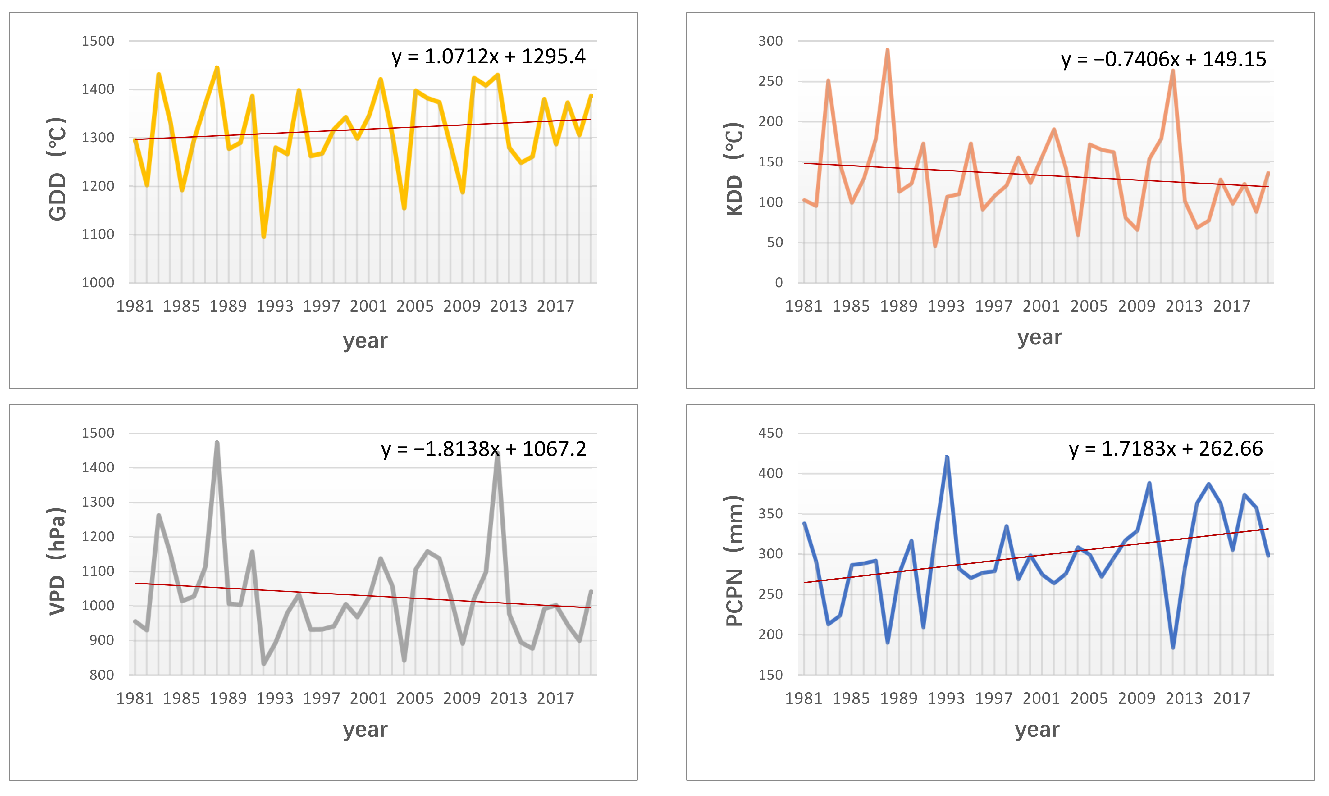
4.1. How Detrended Yield and Meteorological Variables Changed over 40 Years

After applying the linear detrending treatments from 1981 to 2020, the corn yield trends were very flat (Figure 3), indicating that time-dependent factors were almost completely eliminated. As the improvements in production brought about by technological advances and human behavior were removed, we were able to focus on the impact of climate change on yield. In addition, low values fluctuated more widely than high values, indicating that corn yield was susceptible to negative volatility. One of the purposes of this study was, therefore, to reduce the negative impact of meteorological variables on corn yield by determining how climate change affects yields.

Table 2. Correlation analysis results of meteorological variables and detrended yield, with all p-values < 0.001. TEMP_all, GDD_all, KDD_all, VPD_all, and PCPN_all data are aggregated from May 1 to October 31, whereas TEMP_s, GDD_s, KDD_s, VPD_s, and PCPN_s data are aggregated over the summer months of June, July, and August.

	TEMP_all	GDD_all	KDD_all	VPD_all	PCPN_all	TEMP_s	GDD_s	KDD_s	VPD_s	PCPN_s	De-yield
TEMP_all	1.00
GDD_all	1.00	1.00
KDD_all	0.70	0.72	1.00
VPD_all	0.56	0.58	0.92	1.00
PCPN_all	0.20	0.18	−0.26	−0.43	1.00
TEMP_s	0.93	0.95	0.80	0.66	0.10	1.00
GDD_s	0.93	0.95	0.80	0.66	0.10	1.00	1.00
KDD_s	0.67	0.70	0.99	0.91	−0.26	0.80	0.80	1.00
VPD_s	0.46	0.48	0.90	0.96	−0.44	0.61	0.61	0.91	1.00
PCPN_s	0.07	0.06	−0.30	−0.39	0.78	−0.02	−0.02	−0.32	−0.47	1.00
De-yield	−0.06	−0.07	−0.30	−0.26	0.19	−0.17	−0.17	−0.32	−0.32	0.27	1.00

shows the result of correlation analysis for 40 years of 41,693 county-years of recorded yield data along with the TEMP, GDD, KDD, VPD, and PCPN variables aggregated over growing seasons. Traditionally, the growing season for the Corn Belt runs from May 1 to October 31. However, for simplicity, researchers may define the corn growing season as June, July, and August, i.e., the summer [51,52]. We found that all of the meteorological factors in summer had better relevance with the detrended yield than in the growing season, especially for TEMP, GDD, and PCPN.

For temperature-dependent factors in the summer, the correlation coefficient between KDD and the detrended yield was −0.32, which was much higher than the coefficient of −0.17 between both TEMP and GDD and the detrended yield; the correlation between TEMP and GDD was close to 1. All three temperature-related factors were negatively correlated with corn yield. For water-dependent variables, the coefficients of VPD (−0.32) and PCPN (0.27) were not significantly different in terms of absolute value, although the yield was negatively correlated with VPD and positively correlated with PCPN. Ultimately, we chose GDD, KDD, VPD, and PCPN in the summer months as the factors for our next experiment.

From Figure 4, it can be seen that GDD increased over the past 40 years, while KDD decreased. This indicates that although the temperature increased, instances of extremely hot weather decreased, in turn implying that the impact of global warming on the U.S. Corn Belt may not have been completely negative. Furthermore, the upward trend in PCPN and the downward trend in VPD were very clear. Figure 4 shows that the annual distribution of meteorological variables in the Corn Belt was uneven, showing several sudden decreases or increases in accumulated temperature or precipitation between 1981 and 2020. Cumulative temperature GDD and KDD plummeted in 1992, 2004, 2009, and 2014, whereas KDD increased abruptly in 1983, 1988, and 2012, implying that the former years were much cooler and the latter years were hotter than average summers. In 1988 and 2012, there was a sharp rise in VPD and a sudden decline in PCPN, implying extreme dry weather.

Combining the detrended corn yield and meteorological variables, we found a significant nadir in 2012 that coincided with notable heat and drought. In 1983, 1988, 1993, and 2002, when corn production fell deeply, several climate conditions were either higher or lower than normal conditions.

4.2. Spatiotemporal Model Fitting and Performance in Assessing Climate Change Impact on Yield

We applied several spatiotemporal models to the detrended yield and meteorological variables in summer that were chosen in the previous section to fit reliable yield–meteorology relationships. It can be seen from

Table 3. Summary of parameters and performances of ordinary least square (OLS), time linear regression (LR), geographically weighted regression (GWR) with Gaussian kernel, GWR with the bi-square kernel, geographically and temporally weighted regression (GTWR) with Gaussian kernel, and GTWR with bi-square kernel models; values in round brackets are the first and third quantiles of the coefficients.

Parameters	OLS	Time-LR	GWR-Gaussian	GWR-Bi-Square	GTWR-Gaussian	GTWR-Bi-Square
Coefficient of GDD (tons/ha/°C)	0.0012	0.0021 (−0.0003, 0.0044)	0.0019 (−0.0000, 0.0036)	0.0020 (−0.0002, 0.0042)	0.0012 (−0.0016, 0.0039)	0.0010 (−0.0020, 0.0041)
Coefficient of KDD (tons/ha/°C)	−0.0063	−0.0121 (−0.0171, −0.0071)	−0.0114 (−0.0153, −0.0075)	−0.0119 (−0.0168, −0.0072)	−0.0020 (−0.0016, −0.0060)	−0.0017 (−0.0106, 0.0069)
Coefficient of VPD (tons/ha/Pa)	0.0006	−0.0005 (−0.0025, 0.0014)	−0.0005 (−0.0021, 0.0010)	−0.0006 (−0.0024, 0.0013)	−0.0007 (−0.0030, 0.0016)	−0.0006 (−0.0031, 0.0019)
Coefficient of PCPN (tons/ha/mm)	0.0019	0.0004 (−0.0018, 0.0021)	0.0005 (−0.0012, 0.0021)	0.0004 (−0.0016, 0.0020)	0.0022 (−0.0001, 0.0041)	0.0022 (−0.0003, 0.0043)
Moran’s I of residuals	0.53	0.44	0.33	0.32	0.22	0.19
Adj.R2	0.14	0.44	0.59	0.63	0.73	0.79
MAE (tons/ha)	0.89	0.74	0.66	0.64	0.50	0.44
RMSE (tons/ha)	1.18	0.96	0.88	0.86	0.67	0.59

that the GTWR outperformed alternative models, namely, OLS, time-LR, and GWR, in fitting corn yield. GTWR had the highest adjusted R² of 0.79, obtained using a bi-square kernel. The GTWR-bi-square had the lowest RMSE of all models, with a value of 0.59 tons/ha. Furthermore, GTWR, which is based on spatiotemporally non-stationary processes, outperformed GWR, which only accounts for spatial autocorrelation, in terms of almost all factors. GTWR similarly outperformed time-LR, which only considers temporal autocorrelation, and OLS, which considers neither autocorrelation. The OLS and time-LR models performed exceptionally poorly compared to other traditional studies, as we used unbalanced data without data completion in order to demonstrate the superiority of the GWR and GTWR models on such tasks.

Based on the Moran’s I of the residuals in Table 3, all of the experimental models were significantly positive, indicating that neighboring counties tended to have similar degrees of estimation bias. As the GTWR model considered spatial autocorrelation, it had fewer spatial clustered residuals. Unexpectedly, incorporating the temporal non-stationarity in the GWR model significantly reduced the spatial autocorrelation of residuals in GTWR to 0.22 and 0.19, compared to 0.33 and 0.32 for the GWR (p < 0.01 for all years and models). These findings prove that temporal non-stationarity plays an important role in resolving spatial autocorrelation.

The improved performance of the GTWR model indicates that non-stationary spatiotemporal processes are more suitable for the description of the relationship between meteorology and yield. GTWR with a bi-square kernel showed a slightly better performance than GTWR with a Gaussian kernel, making the former the best model for our study.

We then used the 40-year average coefficient weights of the meteorological variables obtained from the GTWR-bi-square model, shown in Table 3, to illustrate the general relationship between meteorology and yield. GDD and PCPN had positive effects on yield. For every degree of increase in GDD, the yield increased by 1 kg/ha, while for each millimeter increase in PCPN the yield increased by 2.2 kg/ha. However, the impact of KDD and VPD on yield was negative. Yield decreased by 1.7 or 0.6 kg/ha for every degree increase in KDD or every hectopascal increase in VPD. Coincidentally, combined with the 40-year climate trends shown in Figure 4, we predicted that all four climate variables would have a positive impact on yield in the summer. This implies that nearly 40 years of climate change has had a positive impact on yields in the U.S. Corn Belt.

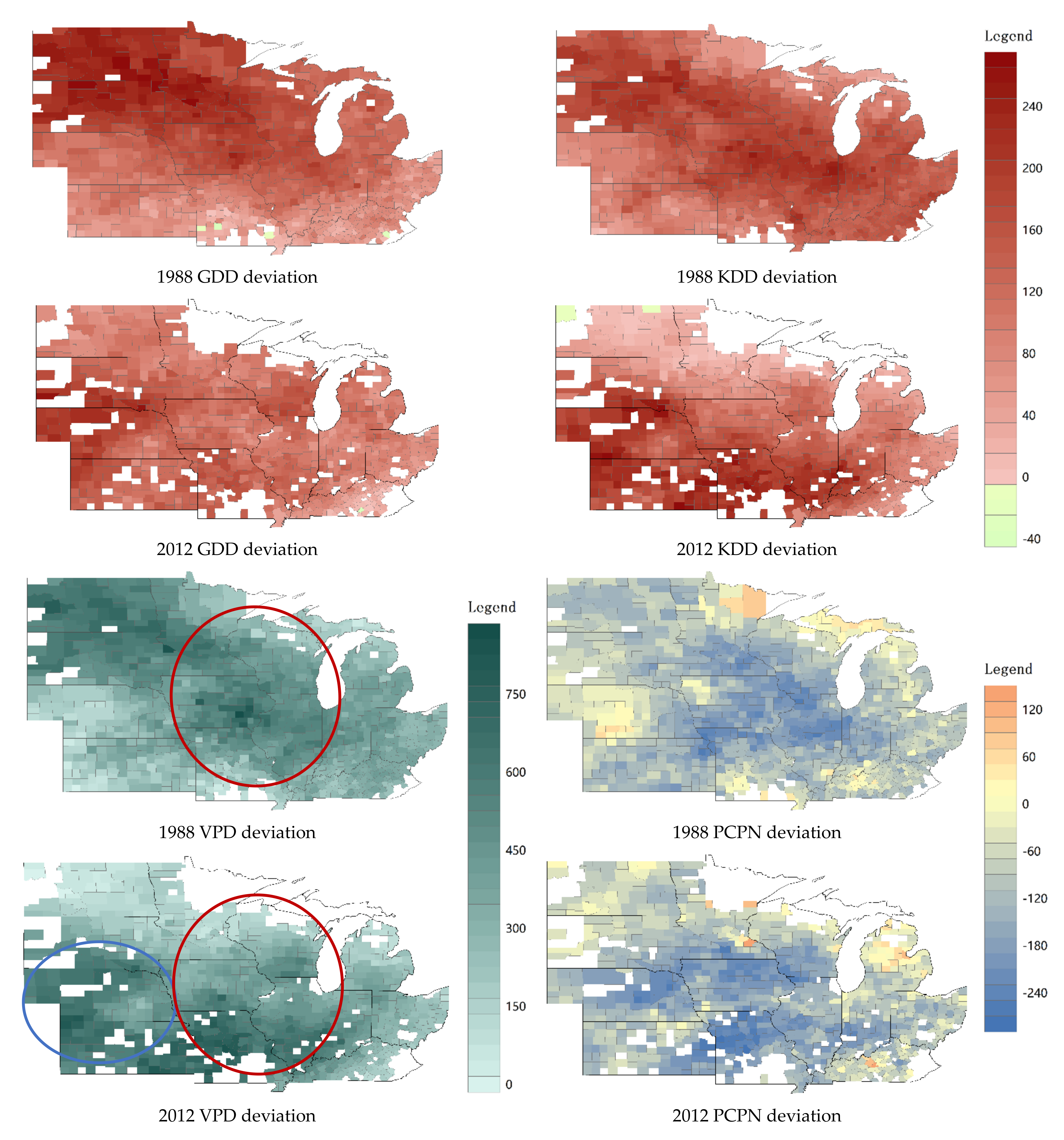
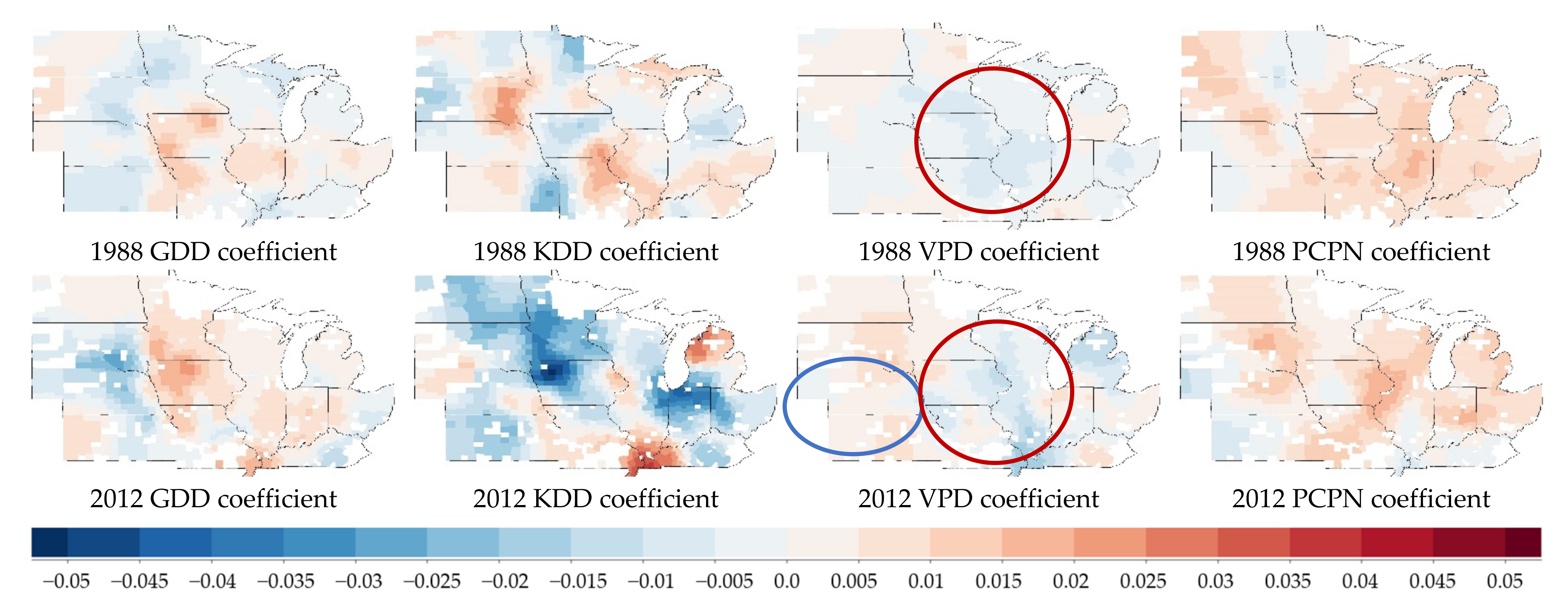
4.3. Explaining Yield Anomalies during Extreme Drought and Hot Climate Events

Historically, droughts have been major contributors to agricultural losses [53,54], and are often accompanied by high temperatures. Corn is especially vulnerable to climate change due to its high irrigation requirements. High temperatures are expected to increase water loss, making corn production susceptible to drought and high temperatures. Thus far, this study has confirmed that latitude and air temperature are closely related, with KDD having the strongest influence. We found that KDD and VPD were highly correlated, with a correlation coefficient of 0.91 in Table 2, indicating that high temperature is often accompanied by high VPD, which inhibits crop growth due to a lack of moisture.

The county-level results for GDD, KDD, VPD, PCPN and detrended yield in 1988 and 2012 are presented in

Table 4. Summary of meteorological variables and detrended yield in 1988 and 2012 at the county level.

Year	County		GDD	KDD	VPD	PCPN	De-Yield
1988	1134	Average over 40 years	1311.5 °C	135.4 °C	1034.1 Pa	294.2 mm	6.33 tons/ha
		Average for 1988	1444.6 °C	289.1 °C	1472.4 Pa	190.3 mm	4.85 tons/ha
		Average deviation	133.1 °C	153.7 °C	438.3 Pa	−103.9 mm	−1.48 tons/ha
		Deviation ratio	10.1%	113.5%	42.4%	−35.3%	−23.4%
		Average of coefficients	0.0003 tons/ha/°C	0.0015 tons/ha/°C	−0.0021 tons/ha/Pa	0.0061 tons/ha/mm	/
2012	996	Average over 40 years	1316.5 °C	134.3 °C	1031.9 Pa	295.3 mm	6.33 tons/ha
		Average for 2012	1431 °C	263.8 °C	1443.4 Pa	184.1 mm	3.83 tons/ha
		Average deviation	114.5 °C	129.5 °C	411.5 Pa	−111.2 mm	−2.50 tons/ha
		Deviation ratio	8.7%	96.4%	39.9%	−37.7%	−39.5%
		Average of coefficients	0.0020 tons/ha/°C	−0.0090 tons/ha/°C	−0.0014 tons/ha/Pa	0.0055 tons/ha/mm	/

. We used these results to determine how extreme drought and hot weather led to a sharp decrease in corn yield. The changes in meteorological variables in the summer for these two years were very similar. Compared with the normal climate, from the attribute of deviation ratio, GDD increased by around 10%, KDD increased by around 100%, VPD increased by around 40%, and PCPN decreased by around 35%, while the difference in detrended yield reduction was almost double. The spatial distributions of deviations in meteorological variables at the county level were quite different between 1988 and 2012, as shown in Figure 5.

Figure 5 shows that the deviation of GDD and KDD to the value of the average over 40 years was lower in most areas in 2012 than in 1988, while the marginal effect was stronger, from 0.3 kg/ha in 1988 to 2 kg/ha in 2012 for a 1 °C increase in GDD and 1.5 kg/ha in 1988 to −9 kg/ha in 2012 for a 1 °C increase in KDD, as shown in Table 4. In terms of GDD, the increase in temperature slightly boosted the yield, while in terms of KDD the extremely high temperature had a significant negative effect in 2012. As can be seen in Figure 6, although the northern regions experienced only slight increases in KDD in 2012, the negative impact was sizeable. This illustrates that higher latitudes experienced a greater impact due to extremely high temperatures, and further indicates that the southern regions had better heat resistance.

Figure 6 shows that the boundary effect of the PCPN coefficient was close to positive on a large scale, with the red part having more area than the blue part. For each additional milliliter of precipitation in Table 4, the yield in 1988 and 2012 increased by 6.1 kg/ha and 5.5 kg/ha, respectively. This indicates that precipitation and yield had a stable positive correlation. The impact of VPD on yield was relatively mild in terms of space in both 1988 and 2012, as shown in Figure 6. Then, as shown in Table 4, the average yield in 1988 and 2012 increased by −2.1 kg/ha and −1.4 kg/ha, respectively. The portion in the red circle in Figure 6 centered on Illinois, Wisconsin, and Iowa experienced a steady negative impact and was very sensitive to VPD. Nebraska and Kansas (blue circle), which are typically irrigated areas [13,55], experienced a very large increase in VPD in Figure 5, and only a small actual impact on yield in Figure 6, especially in 2012. Despite the increase in VPD, the marginal effect remained positive, indicating the significant positive effect of irrigation. Thus, the impact of VPD on yield can be alleviated manually; the effect of irrigation was evident.

In conclusion, the impact of temperature on yield increased between 1988 and 2020 and that of water declined, as it is more amenable to human intervention. Furthermore, we found that the impact of climate factors on yield has a threshold; even though the impact may not necessarily be negative, production is expected to decrease because of declining yields.

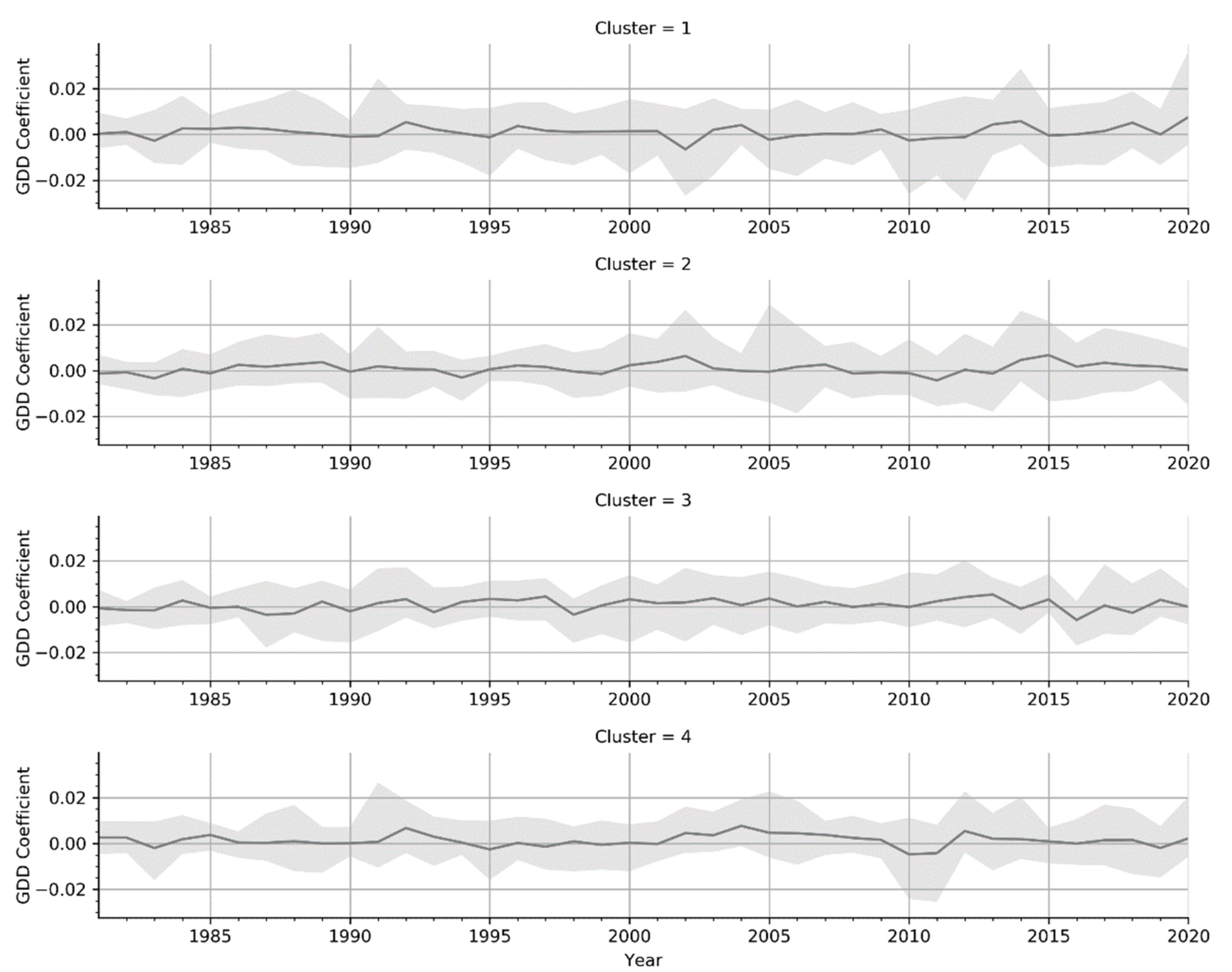
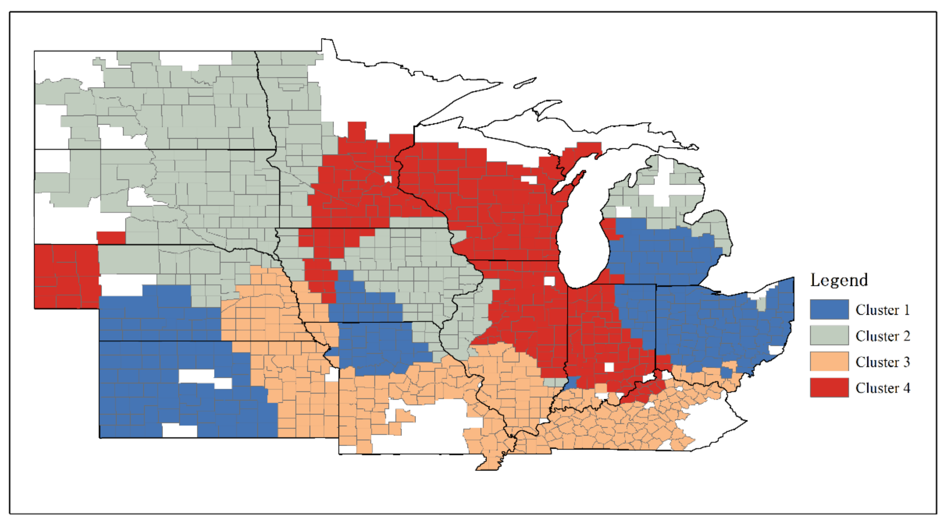
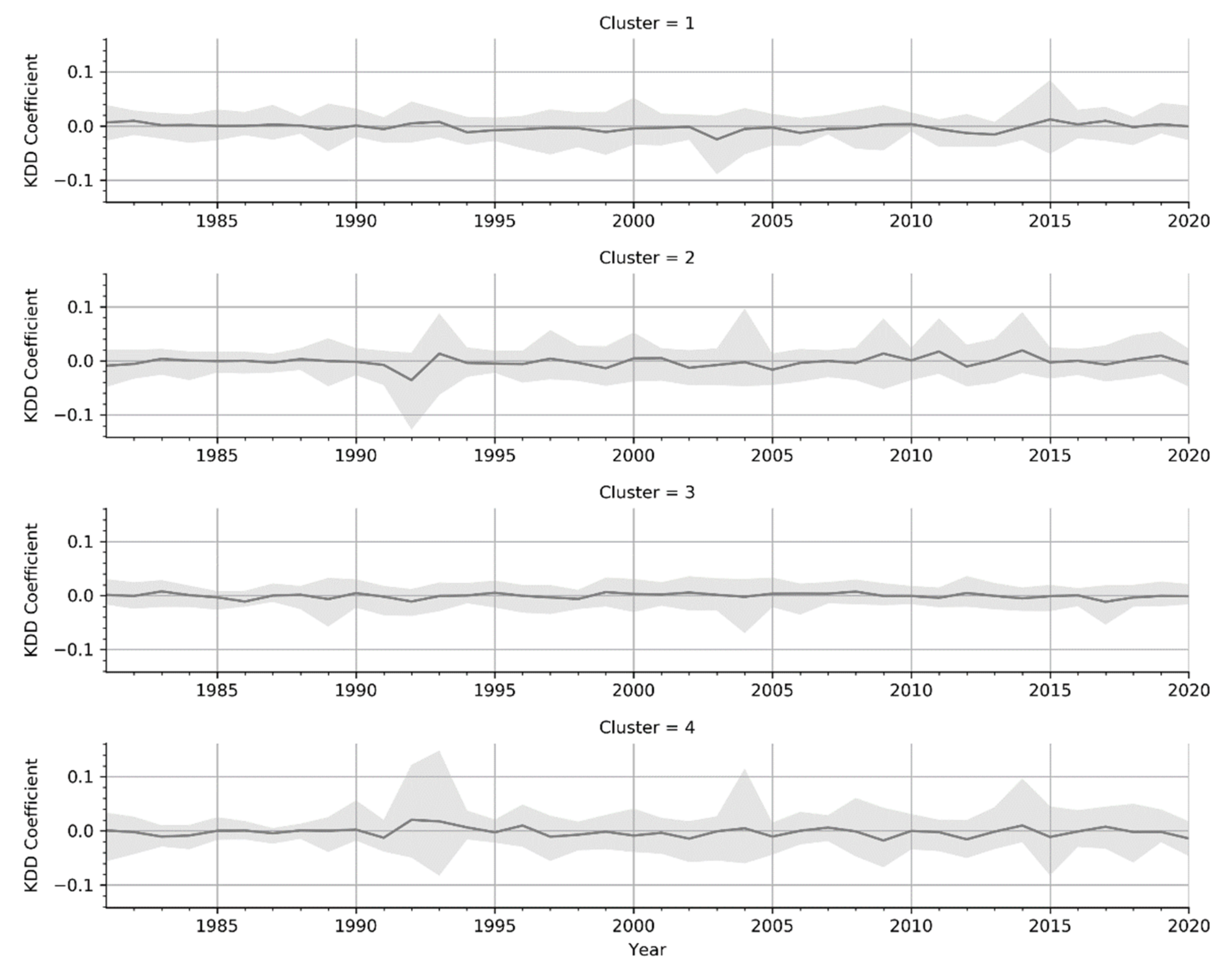
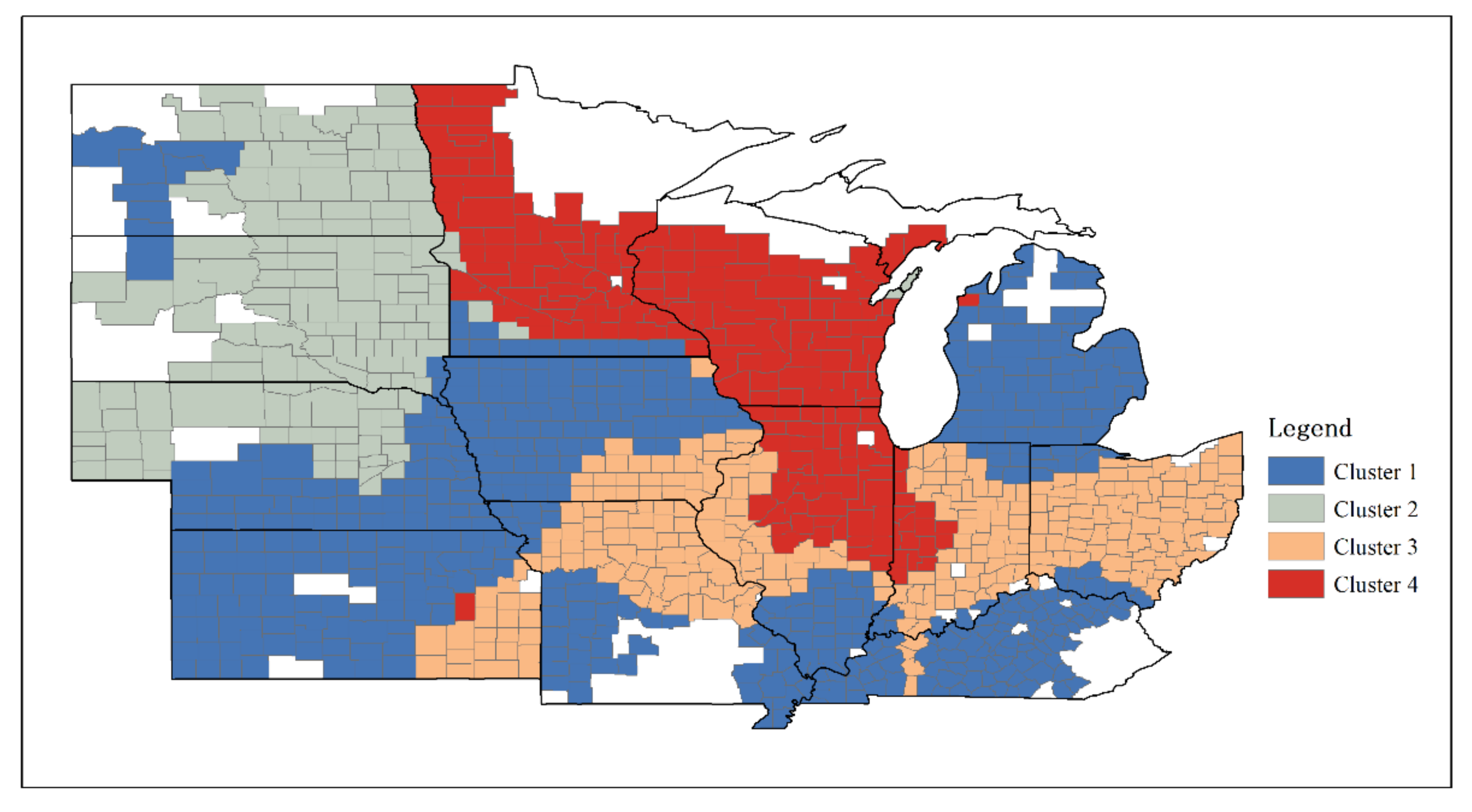
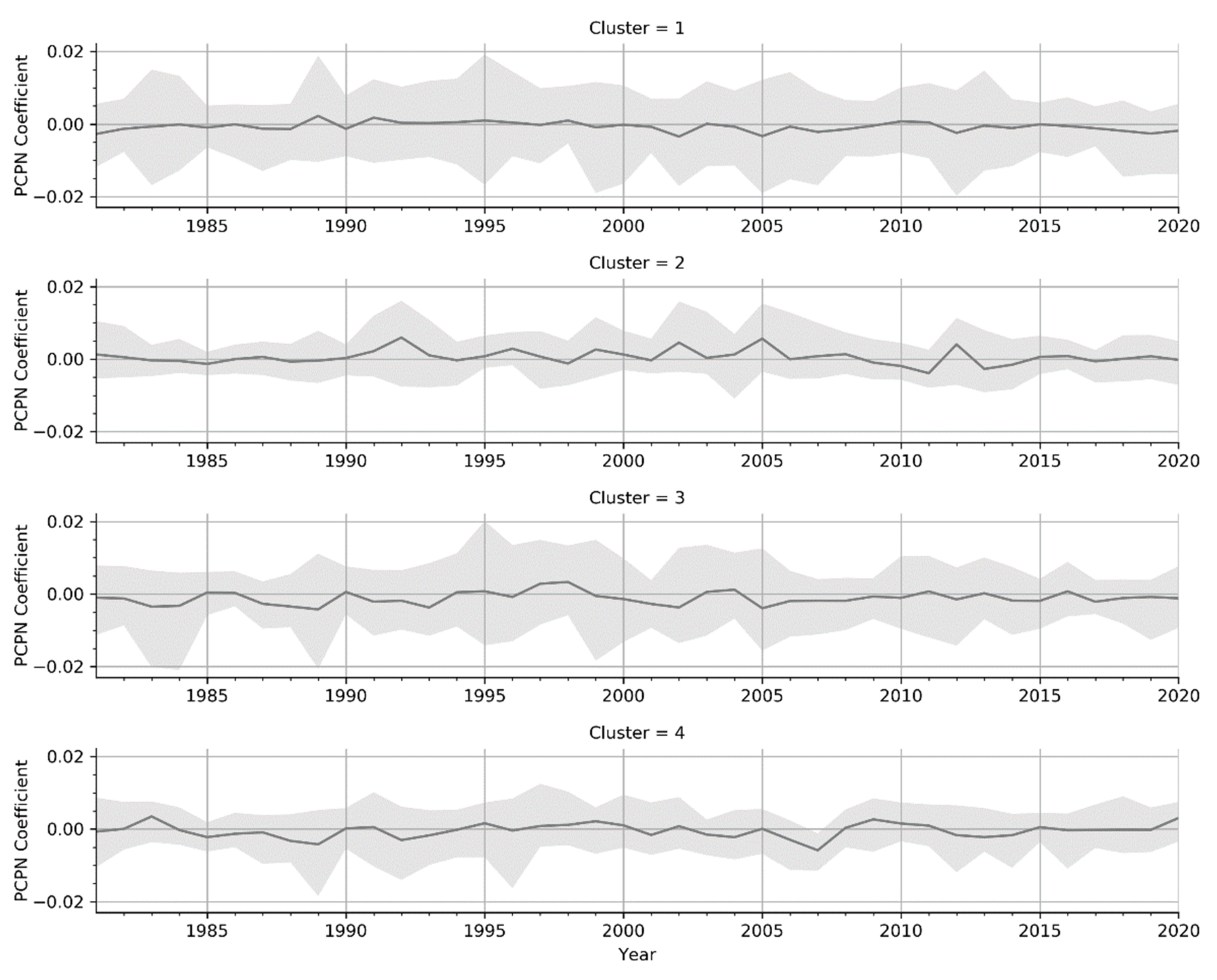
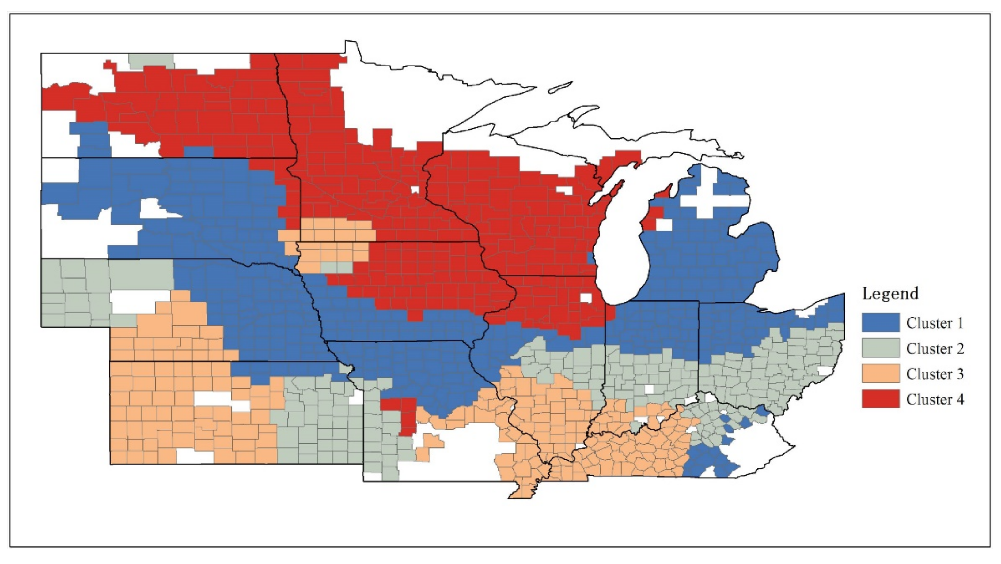
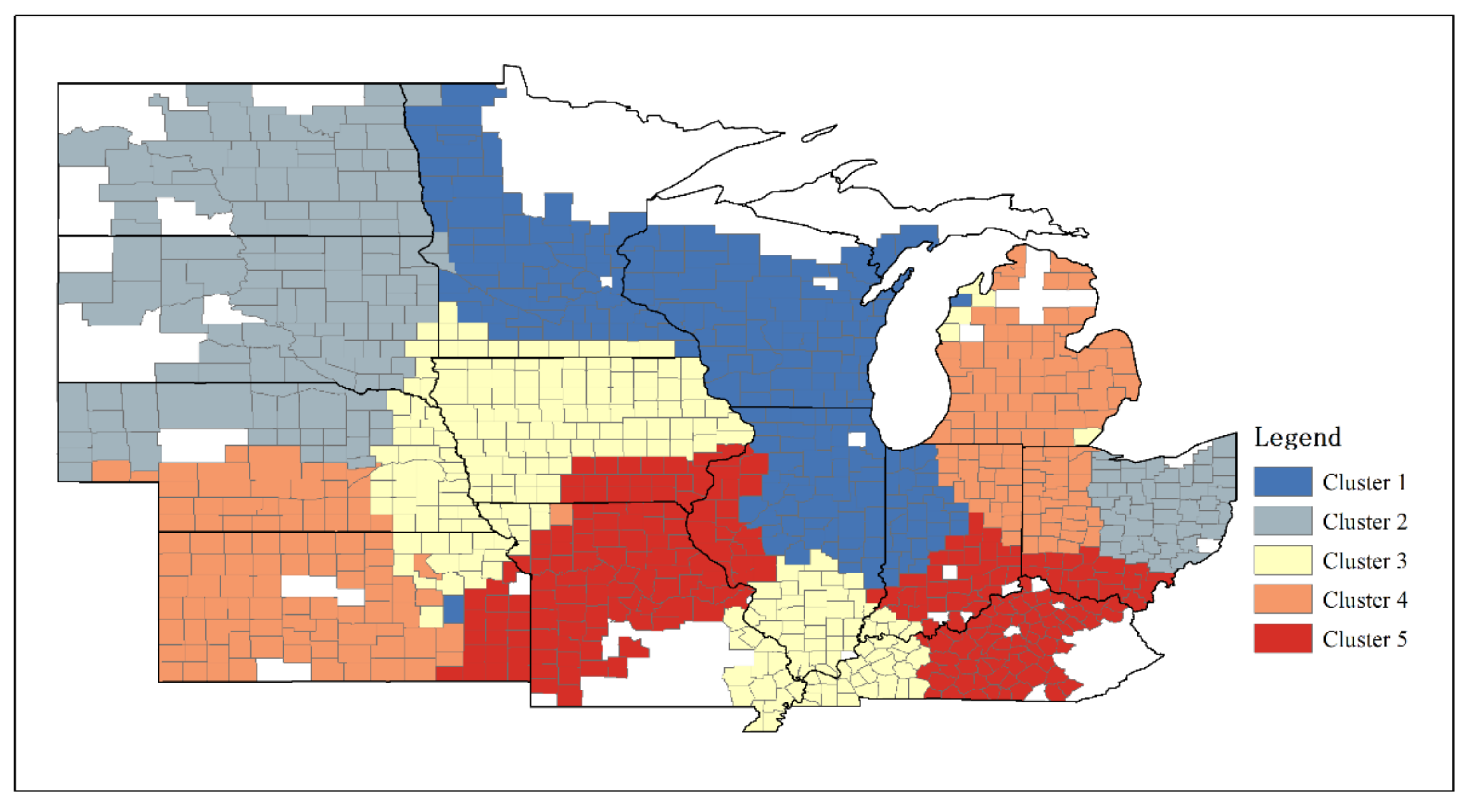
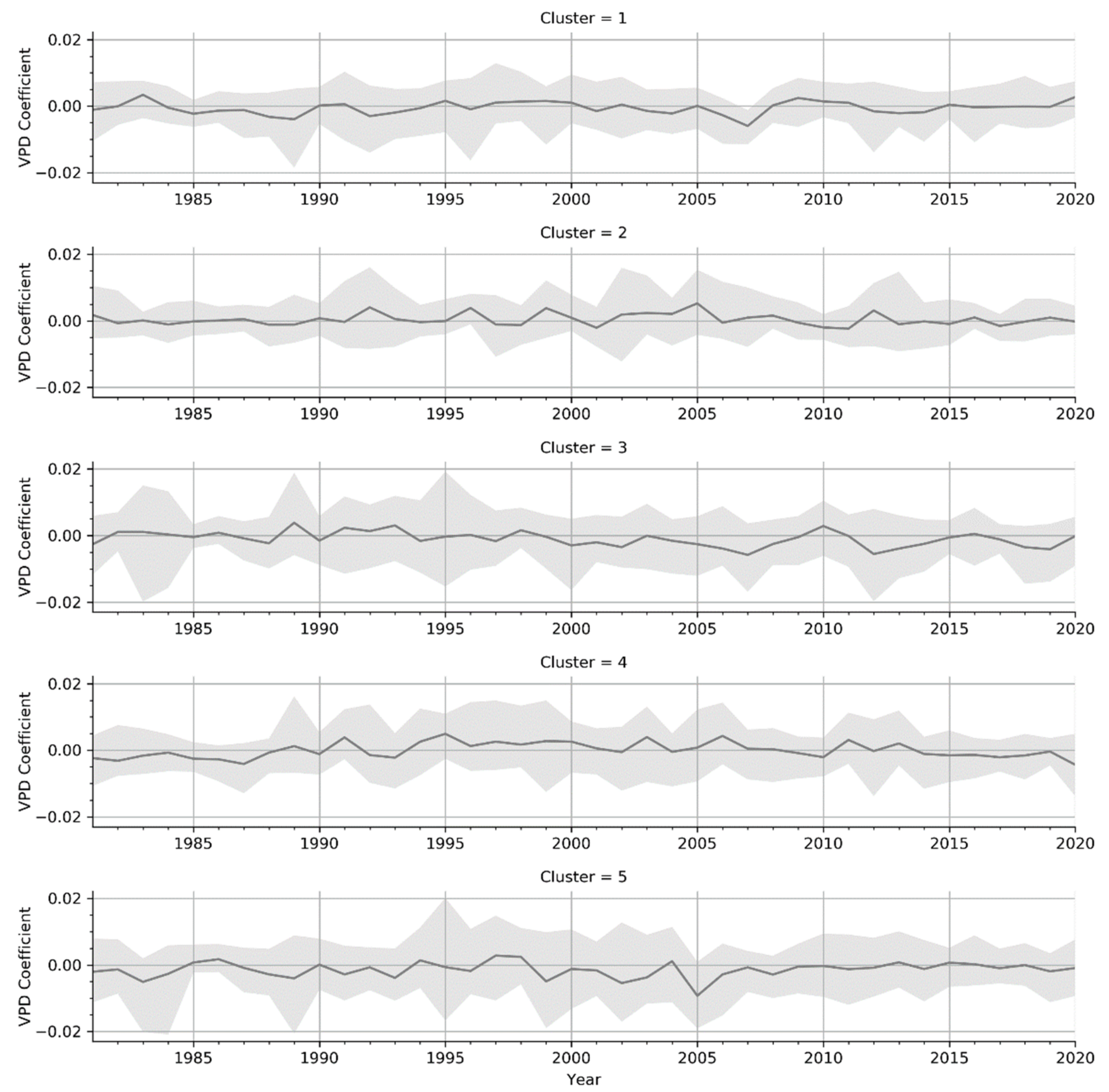
4.4. Temporal and Spatial Clustering Based on Climate Change Impact Trends

We performed fuzzy c-means clustering of the results of the GTWR-bi-square model to obtain the membership values of counties with different meteorological variables for each cluster. As a first step, we excluded 122 counties with more than 25% of the years missing. This left 1037 counties that met the requirements of the Mfuzz clustering method. In order to better understand the experimental results, we divided the effect of GDD on yield from 1981 to 2020 into four clusters, the effect of KDD into four clusters, the effect of VPD into five clusters, and the effect of PCPN into four clusters.

Figure 7 shows that the clustering result for GDD was distributed based on latitude, which was in line with our expectations. Cluster 3, which was located at the lowest latitude, showed relatively stable fluctuations of the boundary effect of yield; its absolute values were low, with most of the values in the range of ±0.01, as shown in Figure 8. Cluster 4, at the highest latitude, showed a clear positive trend between 2001 and 2009 in Figure 8, indicating that GDD played a significant role in promoting the yield in this region in this decade. Overall, Figure 8 shows that all four clusters had more positive than negative portions, although the impact trends across different historical periods were not similar. We found that the differences between these four regions further diverged over the past 20 years, from 2000 to 2020, in Figure 8, making the impact of GDD on yield more unsteady.

The impact of temperature-related factors was very latitude-dependent. The clustering results for KDD were completely different from those for GDD, although they showed latitude correlations, as shown in Figure 9. Cluster 2, with the highest overall latitude, was more prone to frequent positive impact fluctuations when excluding a sudden large negative effect in 1992, as shown in Figure 10. Cluster 3, at the lowest latitude, had most coefficients in the range of −0.02 to 0.02 in Figure 10, reflecting corn production more susceptible to negative effects on KDD. The effect of KDD on yield in clusters 2 and 4, both of which were at high latitudes, varied widely and had values close to 0.2. The variation interval decreased as the latitude decreased, confirming that the lower latitude regions were better able to tolerate KDD changes.

The spatial clustering results of county-level VPD coefficients, shown in Figure 11, were highly consistent with the distribution of irrigation districts in the U.S. Most irrigated areas were spatially covered by clusters 2 and 4, which had VPD coefficients falling within the smallest variation range, as shown in Figure 12. This confirmed that the two regions affected by VPD fluctuated the least. Rainfall in the other three cluster areas was abundant, making irrigation unnecessary. These three clustered regions were strongly affected by VPD and were more susceptible to negative effects. Based on the changing trends over the past ten years shown in Figure 12, the regions in clusters 3 and 4 had reduced resistance to VPD. For the regions in cluster 4, this loss in resistance may have been caused by a drop in the groundwater level, which could have caused irrigation problems. As the regions in cluster 3 are relatively far from both the Great Lakes and the Atlantic Ocean, their declining ability to withstand climate change is understandable. However, production conditions permitting, irrigation technology can be upgraded to supplement these areas.

It is clear that the spatial clustering results for PCPN clusters 2 and 4 in Figure 13 have corresponding regions in clusters 2 and 1 for VPD in Figure 11. This indicates that the moisture-related VPD and PCPN were highly correlated in these two regions. In Figure 14, cluster 2, which required irrigation, had a significant positive feedback effect on corn yield, especially from 1990 to 2010. Cluster 4, which has historically been largely negatively impacted by PCPN, was positively impacted by PCPN over the past five years, even exceeding the positive impact of cluster 2. In addition, the variation interval in Clusters 2 and 4 were smaller than in the other two, illustrating that the high-latitude regions in the Corn Belt had a better tolerance for PCPN changes. In general, the magnitude of the impact faced by the four clusters has reduced in recent years. In contrast, the coefficient variation of PCPN was not as high as that of VPD, which better represented the water-related impact on corn yield.

5. Discussion

This study aimed to discover the temporal and spatial relationships between meteorological variables and corn yield using county-level data from the U.S. Corn Belt. By implementing a spatiotemporal analytical framework based on the GTWR model and fuzzy c-means algorithm, we obtained immediate information. Climate factors had different effects on crop yield at different points in time and space, especially in extremely dry and hot climates in 1988 and 2012. There was a high degree of diversity in the trends with respect to climate change’s impact on yield in different regions. In the future, we can synthesize this information to innovatively discover and discuss these trends and their implications.

5.1. Optimistic Predictions for the Impact of Climate Change on the Corn Belt

First, from the perspective of the whole corn belt region, the impact of climate variables on corn yield showed a positive trend. The coefficients of the GTWR model were positive for GDD and PCPN, and the values increased over time. Although KDD and VPD had negative coefficients, their values decreased over time. Based on the trends in the climate variables in the summer from 1981 to 2020 in Section 4.1 in combination with the coefficients in Section 4.2, GDD promoted corn yield by 0.07 kg/ha, KDD by 2.96 kg/ha, VPD by 1.69 kg/ha, and PCPN by 1.58 kg/ha on average per year.

Fortunately, since 2012, climate change has been relatively mild and conditions have been amenable to the healthy growth of crops. This has resulted in an upward trend in future yield, with production set to increase by 6.30 kg/ha due to climate change.

Researchers have found that precipitation increases yield in nearly all crops and countries [38,46]. Furthermore, although yields tend to be reduced when temperatures rise, this is not necessarily the case in high-latitude countries, where crops particularly benefit from warming [11,35]. Our findings are consistent with previous studies in which crop production at high latitudes such as the Corn Belt in the northern U.S. appeared to benefit from a warming climate [11].

5.2. Temperature Has a Stronger Impact than Precipitation

The ways in which the effects of the climate variables changed over the past four decades year by year have been discussed in Section 5.1. We found that KDD provided the greatest yield boost to productivity, proving that temperature changes were more important than precipitation changes at both national and regional scales [11] as well as at the county scale.

We found evidence to show that the influence of temperature has been strengthening and that of precipitation has been decreasing, especially in extreme climates. For example, in Table 4 of Section 4.3, we showed that KDD caused a crop yield loss of 1165.5 kg/ha in 2012, the effect being far greater than in 1988. Meanwhile, the corn yield loss caused by PCPN slightly decreased, from 633.79 kg/ha in 1988 to 611.6 kg/ha in 2012.

In previous studies, corn has been found to be more vulnerable to climate change due to its high irrigation water requirements [56,57]. However, crop yields could increase by expanding irrigated areas or intensifying irrigation [13,58], reducing the influence of natural rainfall. In this study, we selected a mature and specialized corn-producing area where the irrigation levels were already very professional. Thus, the impact of precipitation on corn yield was lower than that of temperature in our study area.

Despite recent increases in irrigation, crop yield has been reduced due to a lack of rainfall [59]. In addition, the groundwater table, on which irrigation is partly dependent, has been shown to be falling [55,60]. This has made future impact predictions not very optimistic.

5.3. Better Production Potential in High Latitudes

The effects of climate change on crop yield are expected to vary across regions, with crop yield increasing in some regions and decreasing in others, depending on the latitude and irrigation requirements of the region [1].

In Section 4.4, Figure 8 shows that GDD had more positive effects than negative effects on yield in nearly all Corn Belt regions. However, as shown in Figure 9 and Figure 10, the ability of several high-latitude counties, such as those in Wisconsin, Minnesota, North Dakota, and South Dakota, to withstand high temperatures was very low. The loss due to extreme heat in these regions is expected to be high. In contrast, regions at lower latitudes, such as those in Kentucky, Kansas, Missouri, and Southern Illinois, were more tolerant of extreme temperatures.

In terms of water, as shown in Figure 13 and Figure 14, most high-latitude regions were less sensitive to precipitation. Overall, selecting more heat-tolerant corn varieties or implementing greenhouse cultivation, thereby reducing the sensitivity to KDD, may contribute to greater increases in corn yield in high-latitude regions. This would mean that regions at higher latitudes would have a stronger potential to increase production despite climate change compared to those at lower latitudes.

6. Conclusions and Future Works

We applied a spatiotemporal analytical framework largely based on the GTWR model to a sample of 1159 counties in the U.S. Corn Belt, covering 13 States from 1981 to 2020. The results showed how four main meteorological variables quantitatively and qualitatively impacted corn production.

The GTWR model, which combines all data into a single regression, requires little data preprocessing, such as data completion for counties with missing years; this helps to remove human interference from the analysis of spatiotemporal relationships. Compared to previous studies, the completeness and accuracy of the original unbalanced data allowed us to obtain a more accurate prediction of climate responses. By accounting for both spatial and temporal non-stationary relationships, we were able to efficiently and robustly handle the spatiotemporal heterogeneity of the climate data.

Using the powerful spatiotemporal regression tool of the GTWR model, we innovatively uncovered several relationships between climate change and corn yield that varied over time and space. Temporally, the U.S. Corn Belt has benefited from the increase in temperature and precipitation over the past four decades, with the temperature effect being larger. Moreover, the impact of precipitation on yield decreased, whereas that of temperature increased during extreme climate events, mainly due to the use of artificial irrigation as a water supplement. Spatially, the impact of climate change on yield was closely related to latitude, with the production potential being higher in high-latitude areas.

Although we obtained large amounts of information from the spatiotemporal analytical model, the degree of information mining was not deep enough and the direction was not comprehensive. Meanwhile, this paper lacks simulations for projected climate change scenarios, which could have widened the information presented in the regression analysis with the historical meteorological data. In the future, we will try to find more patterns between climate change and crop yield. In addition, this model can be applied to other regions in order to further test its robustness and effectiveness.

References

1. Kang, Y.; Khan, S.; Ma, X. Climate change impacts on crop yield, crop water productivity and food security—A review. Prog. Nat. Sci. 2009, 19, 1665–1674. [Google Scholar] [CrossRef]
2. Lobell, D.B.; Burke, M.B. On the use of statistical models to predict crop yield responses to climate change. Agric. For. Meteorol. 2010, 150, 1443–1452. [Google Scholar] [CrossRef]
3. Monfreda, C.; Ramankutty, N.; Foley, J.A. Farming the planet: 2. Geographic distribution of crop areas, yields, physiological types, and net primary production in the year 2000. Glob. Biogeochem. Cycles 2008, 22, 2007GB002947. [Google Scholar] [CrossRef]
4. Tao, F.; Zhang, Z.; Zhang, S.; Rötter, R.P.; Shi, W.; Xiao, D.; Liu, Y.; Wang, M.; Liu, F.; Zhang, H. Historical data provide new insights into response and adaptation of maize production systems to climate change/variability in China. Field Crops Res. 2016, 185, 1–11. [Google Scholar] [CrossRef]
5. Alahacoon, N.; Edirisinghe, M. Spatial Variability of Rainfall Trends in Sri Lanka from 1989 to 2019 as an Indication of Climate Change. ISPRS Int. J Geo-Inf. 2021, 10, 84. [Google Scholar] [CrossRef]
6. Jiang, H.; Hu, H.; Li, B.; Zhang, Z.; Wang, S.; Lin, T. Understanding the non-stationary relationships between corn yields and meteorology via a spatiotemporally varying coefficient model. Agric. For. Meteorol. 2021, 301–302, 108340. [Google Scholar] [CrossRef]
7. Bakhsh, A.; Jaynes, D.B.; Colvin, T.S.; Kanwar, R.S. Spatio-temporal analysis of yield variability for a corn-soybean field in iowa. Trans. ASAE 2000, 43, 31–38. [Google Scholar] [CrossRef]
8. Williams, C.; Hargrove, W.; Liebman, M.; James, D. Agro-ecoregionalization of Iowa using multivariate geographical clustering. Agric. Ecosyst. Environ. 2008, 123, 161–174. [Google Scholar] [CrossRef]
9. Foley, J.A.; Ramankutty, N.; Brauman, K.A.; Cassidy, E.S.; Gerber, J.S.; Johnston, M.; Mueller, N.D.; O Connell, C.; Ray, D.K.; West, P.C.; et al. Solutions for a cultivated planet. Nature 2011, 478, 337–342. [Google Scholar] [CrossRef] [Green Version]
10. Peng, B.; Guan, K.; Tang, J.; Ain Sw Orth, E.A.; Zhou, W. Towards a multiscale crop modelling framework for climate change adaptation assessment. Nat. Plants 2020, 6, 338–348. [Google Scholar] [CrossRef]
11. Lobell, D.B.; Schlenker, W.; Costa-Roberts, J. Climate trends and global crop production since 1980. Science 2011, 333, 616–620. [Google Scholar] [CrossRef] [Green Version]
12. Troy, T.J.; Kipgen, C.; Pal, I. The impact of climate extremes and irrigation on US crop yields. Environ. Res. Lett. 2015, 10, 54013. [Google Scholar] [CrossRef] [Green Version]
13. Morell, F.J.; Yang, H.S.; Cassman, K.G.; Wart, J.V.; Elmore, R.W.; Licht, M.; Coulter, J.A.; Ciampitti, I.A.; Pittelkow, C.M.; Brouder, S.M.; et al. Can crop simulation models be used to predict local to regional maize yields and total production in the U.S. Corn Belt? Field Crops Res. 2016, 192, 1–12. [Google Scholar] [CrossRef] [Green Version]
14. Li, Y.; Guan, K.; Schnitkey, G.D.; Delucia, E.; Peng, B. Excessive rainfall leads to maize yield loss of a comparable magnitude to extreme drought in the United States. Glob. Chang. Biol. 2019, 25, 2325–2337. [Google Scholar] [CrossRef] [Green Version]
15. Blanc, É. Statistical emulators of maize, rice, soybean and wheat yields from global gridded crop models. Agric. For. Meteorol. 2017, 236, 145–161. [Google Scholar] [CrossRef]
16. Cai, R.; Yu, D.; Oppenheimer, M. Estimating the Spatially Varying Responses of Corn Yields to Weather Variations using Geographically Weighted Panel Regression. J. Agric. Resour. Econ. 2014, 39, 230–252. [Google Scholar]
17. Mcgrath, J.M.; Betzelberger, A.M.; Wang, S.; Shook, E.; Ainsworth, E.A. An analysis of ozone damage to historical maize and soybean yields in the United States. Proc. Natl. Acad. Sci. USA 2015, 112, 14390. [Google Scholar] [CrossRef] [Green Version]
18. White, J.W.; Hoogenboom, G.; Kimball, B.A.; Wall, G.W. Methodologies for simulating impacts of climate change on crop production. Field Crops Res. 2011, 124, 357–368. [Google Scholar] [CrossRef] [Green Version]
19. Jones, J.W.; Hoogenboom, G.; Porter, C.H.; Boote, K.J.; Batchelor, W.D.; Hunt, L.A.; Wilkens, P.W.; Singh, U.; Gijsman, A.J.; Ritchie, J.T. The DSSAT cropping system model. Eur. J. Agron. 2003, 18, 235–265. [Google Scholar] [CrossRef]
20. Ray, D.K.; Gerber, J.S.; MacDonald, G.K.; West, P.C. Climate variation explains a third of global crop yield variability. Nat. Commun. 2015, 6, 5989. [Google Scholar] [CrossRef] [Green Version]
21. Haghverdi, A.; Leib, B.; Washington-Allen, R.; Wright, W.; Ghodsi, S.; Grant, T.; Zheng, M.; Vanchiasong, P. Studying Crop Yield Response to Supplemental Irrigation and the Spatial Heterogeneity of Soil Physical Attributes in a Humid Region. Agriculture 2019, 9, 43. [Google Scholar] [CrossRef] [Green Version]
22. Choi, J.; Lawson, A.B.; Cai, B.; Hossain, M.M.; Kirby, R.S.; Liu, J. A Bayesian latent model with spatio-temporally varying coefficients in low birth weight incidence data. Statal Methods Med. Res. 2012, 21, 445–456. [Google Scholar] [CrossRef] [PubMed] [Green Version]
23. Folberth, C.; Baklanov, A.; Balkovič, J.; Skalský, R.; Khabarov, N.; Obersteiner, M. Spatio-temporal downscaling of gridded crop model yield estimates based on machine learning. Agric. For. Meteorol. 2018, 264, 1–15. [Google Scholar] [CrossRef] [Green Version]
24. Mahalingam, B.; Orman, W.H. GDP and energy consumption: A panel analysis of the US. Appl. Energy 2018, 213, 208–218. [Google Scholar] [CrossRef]
25. Congdon, P. Analysis of panel data. In Applied Bayesian Modelling; John Wiley & Sons: Hoboken, NJ, USA, 2014. [Google Scholar]
26. Anselin, L.; Gallo, J.L.; Jayet, H. Spatial Panel Econometrics. In The Econometrics of Panel Data; Springer: Berlin/Heidelberg, Germany, 2008; pp. 625–660. [Google Scholar]
27. Olgun, M.; Erdogan, S. Modeling crop yield potential of Eastern Anatolia by using geographically weighted regression. Arch. Acker Pflanzenbau Bodenkd. 2009, 55, 255–263. [Google Scholar] [CrossRef]
28. Duan, P.; Qin, L.; Wang, Y.; He, H. Spatiotemporal Correlations between Water Footprint and Agricultural Inputs: A Case Study of Maize Production in Northeast China. Water 2015, 7, 4026–4040. [Google Scholar] [CrossRef] [Green Version]
29. Yu, D. Exploring Spatiotemporally Varying Regressed Relationships: The Geographically Weighted Panel Regression Analysis. In Proceedings of the Joint International Conference on Theory, Data Handling and Modelling in GeoSpatial Information Science, Hong Kong, 26–28 May 2010; Volume 38, pp. 134–139. [Google Scholar]
30. Huang, B.; Wu, B.; Barry, M. Geographically and temporally weighted regression for modeling spatio-temporal variation in house prices. Int. J. Geogr. Inf. Sci. IJGIS 2010, 24, 383–401. [Google Scholar] [CrossRef]
31. Wu, B.; Li, R.; Huang, B. A geographically and temporally weighted autoregressive model with application to housing prices. Int. J. Geogr. Inf. Sci. IJGIS 2014, 28, 1186–1204. [Google Scholar] [CrossRef]
32. Fotheringham, A.S.; Crespo, R.; Yao, J. Geographical and Temporal Weighted Regression (GTWR). Geogr. Anal. 2015, 47, 431–452. [Google Scholar] [CrossRef] [Green Version]
33. Du, Z.; Wu, S.; Kwan, M.; Zhang, C.; Zhang, F.; Liu, R. A spatiotemporal regression-kriging model for space-time interpolation: A case study of chlorophyll-a prediction in the coastal areas of Zhejiang, China. Int. J. Geogr. Inf. Sci. IJGIS 2018, 32, 1927–1947. [Google Scholar] [CrossRef]
34. Liu, B.; Asseng, S.; Müller, C.; Ewert, F.; Elliott, J.; Lobell, D.B.; Martre, P.; Ruane, A.C.; Wallach, D.; Jones, J.W.; et al. Similar estimates of temperature impacts on global wheat yield by three independent methods. Nat. Clim. Chang. 2016, 6, 1130–1136. [Google Scholar] [CrossRef]
35. Sacks, W.J.; Kucharik, C.J. Crop management and phenology trends in the U.S. Corn Belt: Impacts on yields, evapotranspiration and energy balance. Agric. For. Meteorol. 2011, 151, 882–894. [Google Scholar] [CrossRef]
36. Sakamoto, T.; Gitelson, A.A.; Arkebauer, T.J. MODIS-based corn grain yield estimation model incorporating crop phenology information. Remote Sens. Environ. 2013, 131, 215–231. [Google Scholar] [CrossRef]
37. Buhiniček, I.; Kaučić, D.; Kozić, Z.; Jukić, M.; Gunjača, J.; Šarčević, H.; Stepinac, D.; Šimić, D. Trends in Maize Grain Yields across Five Maturity Groups in a Long-Term Experiment with Changing Genotypes. Agriculture 2021, 11, 887. [Google Scholar] [CrossRef]
38. Lu, J.; Carbone, G.J.; Gao, P. Detrending crop yield data for spatial visualization of drought impacts in the United States, 1895–2014. Agric. For. Meteorol. 2017, 237–238, 196–208. [Google Scholar] [CrossRef]
39. Quiring, S.M.; Papakryiakou, T.N. An evaluation of agricultural drought indices for the Canadian prairies. Agric. For. Meteorol. 2003, 118, 49–62. [Google Scholar] [CrossRef]
40. Mcmaster, G.S.; Wilhelm, W.W. Growing degree-days: One equation, two interpretations. Agric. For. Meteorol. 1997, 87, 291–300. [Google Scholar] [CrossRef] [Green Version]
41. Butler, E.E.; Huybers, P. Adaptation of US maize to temperature variations. Nat. Clim. Chang. 2013, 3, 68–72. [Google Scholar] [CrossRef]
42. Schlenker, W.; Roberts, M.J. Nonlinear temperature effects indicate severe damages to U.S. crop yields under climate change. Proc. Natl. Acad. Sci. USA 2009, 106, 15594–15598. [Google Scholar] [CrossRef] [Green Version]
43. Brunsdon, C.; Fotheringham, A.S.; Charlton, M.E. Geographically weighted regression. Ðmodelling spatial non-stationarity. J. R. Stat. Soc. Ser. D 1998, 47, 431–443. [Google Scholar] [CrossRef]
44. Fotheringham, A.S.; Brunsdon, C.F.; Charlton, M.E. Geographically Weighted Regression: The Analysis of Spatially Varying Relationships; John Wiley & Sons: Hoboken, NJ, USA, 2003. [Google Scholar]
45. Pascucci, S.; Carfora, M.; Palombo, A.; Pignatti, S.; Casa, R.; Pepe, M.; Castaldi, F. A Comparison between Standard and Functional Clustering Methodologies: Application to Agricultural Fields for Yield Pattern Assessment. Remote Sens. 2018, 10, 585. [Google Scholar] [CrossRef] [Green Version]
46. Heinemann, A.B.; Ramirez-Villegas, J.; Souza, T.L.P.O.; Didonet, A.D.; di Stefano, J.G.; Boote, K.J.; Jarvis, A. Drought impact on rainfed common bean production areas in Brazil. Agric. For. Meteorol. 2016, 225, 57–74. [Google Scholar] [CrossRef] [Green Version]
47. Wang, J.; Zhang, J.; Bai, Y.; Zhang, S.; Yang, S.; Yao, F. Integrating remote sensing-based process model with environmental zonation scheme to estimate rice yield gap in Northeast China. Field Crops Res. 2020, 246, 107682. [Google Scholar] [CrossRef]
48. Luo, W.; Yu, Z.; Xiao, S.; Zhu, A.; Yuan, L. Exploratory Method for Spatio-Temporal Feature Extraction and Clustering: An Integrated Multi-Scale Framework. ISPRS Int. J. Geo-Inf. 2015, 4, 1870–1893. [Google Scholar] [CrossRef]
49. Chen, Z.; Ma, X.; Wu, L.; Xie, Z. An Intuitionistic Fuzzy Similarity Approach for Clustering Analysis of Polygons. ISPRS Int. J. Geo-Inf. 2019, 8, 98. [Google Scholar] [CrossRef] [Green Version]
50. Liu, Y.; Yuan, Y.; Gao, S. Modeling the Vagueness of Areal Geographic Objects: A Categorization System. ISPRS Int. J. Geo-Inf. 2019, 8, 306. [Google Scholar] [CrossRef] [Green Version]
51. Rattalino Edreira, J.I.; Mourtzinis, S.; Conley, S.P.; Roth, A.C.; Ciampitti, I.A.; Licht, M.A.; Kandel, H.; Kyveryga, P.M.; Lindsey, L.E.; Mueller, D.S.; et al. Assessing causes of yield gaps in agricultural areas with diversity in climate and soils. Agric. For. Meteorol. 2017, 247, 170–180. [Google Scholar] [CrossRef]
52. Pede, T.; Mountrakis, G.; Shaw, S.B. Improving corn yield prediction across the US Corn Belt by replacing air temperature with daily MODIS land surface temperature. Agric. For. Meteorol. 2019, 276–277, 107615. [Google Scholar] [CrossRef]
53. Lobell, D.B.; Roberts, M.J.; Schlenker, W.; Braun, N.; Little, B.B.; Rejesus, R.M.; Hammer, G.L. Greater Sensitivity to Drought Accompanies Maize Yield Increase in the U.S. Midwest. Science 2014, 344, 516–519. [Google Scholar] [CrossRef]
54. Wei, C.; Liu, C.; Gui, F. Geographically weight seemingly unrelated regression (GWSUR): A method for exploring spatio-temporal heterogeneity. Appl. Econ. 2017, 49, 4189–4195. [Google Scholar] [CrossRef]
55. Mathieu, J.A.; Aires, F. Assessment of the agro-climatic indices to improve crop yield forecasting. Agric. For. Meteorol. 2018, 253–254, 15–30. [Google Scholar] [CrossRef]
56. Gohari, A.; Eslamian, S.; Abedi-Koupaei, J.; Massah Bavani, A.; Wang, D.; Madani, K. Climate change impacts on crop production in Iran’s Zayandeh-Rud River Basin. Sci. Total Environ. 2013, 442, 405–419. [Google Scholar] [CrossRef]
57. Odgaard, M.V.; Bøcher, P.K.; Dalgaard, T.; Svenning, J. Climatic and non-climatic drivers of spatiotemporal maize-area dynamics across the northern limit for maize production—A case study from Denmark. Agric. Ecosyst. Environ. 2011, 142, 291–302. [Google Scholar] [CrossRef]
58. Kassie, B.T.; Van Ittersum, M.K.; Hengsdijk, H.; Asseng, S.; Wolf, J.; Rötter, R.P. Climate-induced yield variability and yield gaps of maize (Zea mays L.) in the Central Rift Valley of Ethiopia. Field Crops Res. 2014, 160, 41–53. [Google Scholar] [CrossRef]
59. Shrestha, D.; Brown, J.F.; Benedict, T.D.; Howard, D.M. Exploring the Regional Dynamics of U.S. Irrigated Agriculture from 2002 to 2017. Land 2021, 10, 394. [Google Scholar] [CrossRef]
60. Orduña Alegría, M.E.; Schütze, N.; Niyogi, D. Evaluation of Hydroclimatic Variability and Prospective Irrigation Strategies in the U.S. Corn Belt. Water 2019, 11, 2447. [Google Scholar] [CrossRef] [Green Version]
Figure 1. Location of the Corn Belt.
Ijgi 11 00433 g001
Figure 2. Experimental procedures.
Ijgi 11 00433 g002
Figure 3. Detrended corn yield (de_yield) from year 1981 to 2020, with the trend line shown in red.
Ijgi 11 00433 g003
Figure 4. Changes in meteorological variables over the summer months from 1981 to 2020.
Ijgi 11 00433 g004
Figure 5. Spatial distributions of deviations in meteorological variables in the summer months at the county level in 1988 and 2012.
Ijgi 11 00433 g005
Figure 6. County-level coefficients from the geographically and temporally weighted regression (GTWR) bi-square model of GDD, KDD, VPD, and PCPN in 1988 and 2012.
Ijgi 11 00433 g006
Figure 7. Four spatial clusters of county-level coefficients of GDD.
Ijgi 11 00433 g007
Figure 8. Impact trends of GDD from 1981 to 2020 for four clusters.
Ijgi 11 00433 g008
Figure 9. Four spatial clusters of county-level coefficients of KDD.
Ijgi 11 00433 g009
Figure 10. Impact trends of KDD from 1981 to 2020 for four clusters.
Ijgi 11 00433 g010
Figure 11. Five spatial clusters of county-level coefficients of VPD.
Ijgi 11 00433 g011
Figure 12. Impact trends of VPD from 1981 to 2020 for five clusters.
Ijgi 11 00433 g012
Figure 13. Four spatial clusters of county-level coefficients of PCPN.
Ijgi 11 00433 g013
Figure 14. Impact trends of PCPN from 1981 to 2020 for four clusters.
Ijgi 11 00433 g014