Article

Global Spatial Suitability Mapping of Wind and Solar Systems Using an Explainable AI-Based Approach

by
Mourtadha Sarhan Sachit
1,2,
Helmi Zulhaidi Mohd Shafri
1,*,
Ahmad Fikri Abdullah
3,
Azmin Shakrine Mohd Rafie
4 and
Mohamed Barakat A. Gibril
1,5
1
Department of Civil Engineering and Geospatial Information Science Research Center (GISRC), Faculty of Engineering, Universiti Putra Malaysia (UPM), Serdang 43400, Malaysia
2
Department of Civil Engineering, College of Engineering, University of Thi-Qar, Nasiriyah 64001, Iraq
3
Institut Antarabangsa Akuakultur dan Sains Akuatik (I-AQUAS), Universiti Putra Malaysia (UPM), Si Rusa 71050, Malaysia
4
Department of Aerospace Engineering, Faculty of Engineering, Universiti Putra Malaysia (UPM), Serdang 43400, Malaysia
5
GIS & Remote Sensing Center, Research Institute of Sciences and Engineering, University of Sharjah, Sharjah P.O. Box 27272, United Arab Emirates
*
Author to whom correspondence should be addressed.
ISPRS Int. J. Geo-Inf. 2022, 11(8), 422; https://doi.org/10.3390/ijgi11080422
Submission received: 13 May 2022 / Revised: 27 June 2022 / Accepted: 8 July 2022 / Published: 26 July 2022
(This article belongs to the Special Issue Upscaling AI Solutions for Large Scale Mapping Applications)

Abstract

:
An assessment of site suitability for wind and solar plants is a strategic step toward ensuring a low-cost, high-performing, and sustainable project. However, these issues are often handled on a local scale using traditional decision-making approaches that involve biased and non-generalizable weightings. This study presents a global wind and solar mapping approach based on eXplainable Artificial Intelligence (XAI). To the best of the author’s knowledge, the current study is the first attempt to create global maps for siting onshore wind and solar power systems and formulate novel weights for decision criteria. A total of 13 conditioning factors (independent variables) defined through a comprehensive literature review and multicollinearity analysis were assessed. Real-world renewable energy experiences (more than 55,000 on-site wind and solar plants worldwide) are exploited to train three machine learning (ML) algorithms, namely Random Forest (RF), Support Vector Machine (SVM), and Multi-layer Perceptron (MLP). Then, the output of ML models was explained using SHapley Additive exPlanations (SHAP). RF outperformed SVM and MLP in both wind and solar modeling with an overall accuracy of 90% and 89%, kappa coefficient of 0.79 and 0.78, and area under the curve of 0.96 and 0.95, respectively. The high and very high suitability categories accounted for 23.2% (~26.84 million km2) of the site suitability map for wind power plants. In addition, they covered more encouraging areas (24.0% and 19.4%, respectively, equivalent to ~50.31 million km2) on the global map for hosting solar energy farms. SHAP interpretations were consistent with the Gini index indicating the dominance of the weights of technical and economic factors over the spatial assessment under consideration. This study provides support to decision-makers toward sustainable power planning worldwide.

1. Introduction

Nowadays, the world faces challenges in meeting the increasing energy demand associated with population explosion and trying to reduce greenhouse gas emissions accompanying these activities [1]. Fortunately, the development of renewable energy (RE) as an essential element of a strategy to mitigate climate change is widely agreed upon [2]. RE’s share in global power generation is projected to increase from the current estimate of 26% to reach 86% by 2050 [3]. Interestingly, wind and solar power are the most mature and popular green energy sources being explored globally owing to their cleanliness degree, availability, capacity factor, and construction cost compared with other clean energy sources [4]. However, extensive lands with special specifications are required to ensure the success of large-scale solar photovoltaic (PV) farms [5]. Similarly, the development of wind plants necessitates careful exploration of sites to meet standard operating conditions [6]. Therefore, a site suitability assessment that considers many aspects is critical in the life cycle of wind and solar systems for a low carbon future.
Traditionally, site suitability for wind and solar plants is assessed using multi-criteria decision-making (MCDM) techniques, such as Analytical Hierarchical Process (AHP) [7,8,9], Technique for Order of Preference by Similarity to Ideal Solution (TOPSIS) [1,10] and fuzzy logic [11,12]. In MCDM-based assessment, criteria are often weighted subjectively or objectively [13]. On the one hand, subjective weighting includes bias, particularly in regions that lack sufficient knowledge maturity of real-world RE experiences to enable local experts to make informed judgments. Objective weighting, on the other hand, is characterized by its inability to generalize, as it can only be applied to pre-determined alternatives. Moreover, the weights change when an alternative is added or deleted [14]. Accordingly, different approaches that provide reliable and generalizable solutions should be adopted.
Recently, machine learning (ML) and geographic information systems (GIS) techniques, along with remote sensing (RS) data, are emerging as among the most appropriate approaches for mapping spatial suitability and hazard susceptibility. ML models have been successfully implemented in many fields to solve location issues, such as predicting suitable sites for dams [15], hospitals [16], solid waste landfills [17], agricultural reclamation [18], and habitats [19]. Meanwhile, interesting attempts have been found to employ ML techniques in selecting optimal sites for RE farms and predicting their renewable resources. For example, a combined approach of AHP weights and suitability classification of the Multi-layer Perceptron (MLP) algorithm was used to locate wind/solar power plants in East Azerbaijan, Iran [20]. The study reported that, by using this procedure, adding a new candidate would not affect the suitability scores of other alternatives. Jani et al. [21] proposed a unique ML-based methodology to select the effective sites for solar and wind simultaneity. In another work covering the USA, the performance of five ML algorithms, namely K-Nearest Neighbors (k-NN), Support Vector Machine (SVM), Decision Tree (DT), Random Forest (RF), and MLP, was analyzed to find the optimal sites against three types of clean energy (wind, solar, and geothermal) [22]. The analysis showed that the RF algorithm performs best with an overall accuracy of 92%. Despite the recommendations of previous work to adopt ML as a viable alternative to MCDM methods, the availability of ground truth samples is a key factor for the smart models to be trained successfully. Thus, the application of these novel techniques for siting wind and solar plants is often not possible in developing countries that have just started planning to rely on green energy sources. Another barrier to the reliable use of ML models in real-world decision-making is the lack of transparency and explainability of the models’ outputs as these are perceived to be black box models [23].
In the last few years, the black box of ML models has been broken by passing on eXplainable Artificial Intelligence (XAI) algorithms, such as SHapley Additive exPlanations (SHAP). XAI refers to AI algorithms in which humans can logically interpret the output at an acceptable level [24]. Explainability facilitates understanding the influence and contribution of each input feature on the AI models’ outputs [25]. Furthermore, XAI has the ability to detect bias in the training dataset, thereby ensuring impartiality in decision-making [26]. XAI has been increasingly applied in the field of spatial prediction of droughts [27,28] and landslides [29], mapping of earthquake-induced building damage [25], and urban vegetation mapping [30]. Most of these studies concluded that XAI can not only provide insight into the output of intelligent models but also change our understanding of using ML-based models to make informed decisions [28]. Considering the aforementioned challenges and opportunities, this paper aims to conduct a GIS-based global assessment using ML and XAI techniques to recognize suitable regions for the development of onshore wind and solar stations. With the holistic vision, the on-site RE experiences worldwide can contribute to mapping spatial appropriateness across the planet, including in developing countries. Such experiences can also generate unbiased weights for decision criteria that can be applied worldwide. To the authors’ knowledge, this study is the first to investigate on a global scale the issue of site suitability for solar and wind energy systems. The specific objectives were to (i) establish a hybrid XAI-GIS framework to select the most suitable locations for RE facilities, considering various geo-technical, economic, and environmental conditioning factors; (ii) perform the suggested framework to generate global maps of site suitability for wind and solar installations; and (iii) discover factor weights influencing the optimal location.

2. Materials and Methods

The methodology developed to assess site suitability for wind and solar plants consists of three main stages, as illustrated in Figure 1. First, efforts are devoted to locating the real-world RE samples and generating thematic layers of conditioning criteria down to extracting a training dataset. The second stage focuses on data preprocessing, which involves refining and optimizing the dataset and dividing it into a train set, validation set and a test set. Finally, the performance of three ML algorithms, namely, RF, MLP, and SVM, is evaluated. The model with high precision metrics is considered for mapping the spatial suitability of wind and solar farms. Moreover, XAI techniques are utilized to interpret the results and derive the global weights for adopted factors. The following subsections discuss the methodology in detail.

2.1. Data Acquisition and Preparation

Two types of data were collected and prepared: an inventory map of the existing solar and wind power plants globally and thematic layers of the conditioning factors. The objective is to train a spatial prediction model for RE farms.

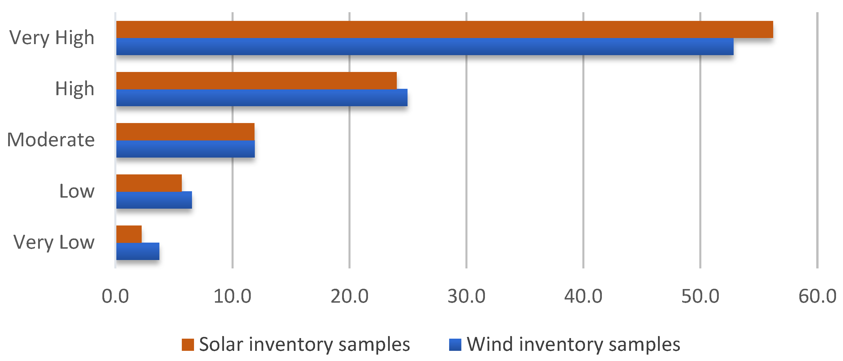
2.1.1. Sample Inventory

The availability of training samples based on real-world experiences is crucial to ensure the success of any ML model [31]. Accordingly, on-site solar and wind installations worldwide are considered samples for training an ML-based spatial assessment model. To this end, spatial data published and publicly available on Figshare entitled “global_wind_solar_2020” are used to inventory the targeted places [32]. These datasets are available in the geopackages and shapefiles format to present the geographic locations of wind turbines and solar panels individually or as groups. Sites’ description, whether urban or next to/on a water body, is included in the metadata of this database. According to the scope of this study, places that are described as urban or on a water body are excluded. All locations above 60° N or below 60° S latitude are also omitted. The total number of wind and solar energy locations considered in this study are 31,571 and 24,048, respectively, as illustrated in Figure 2.

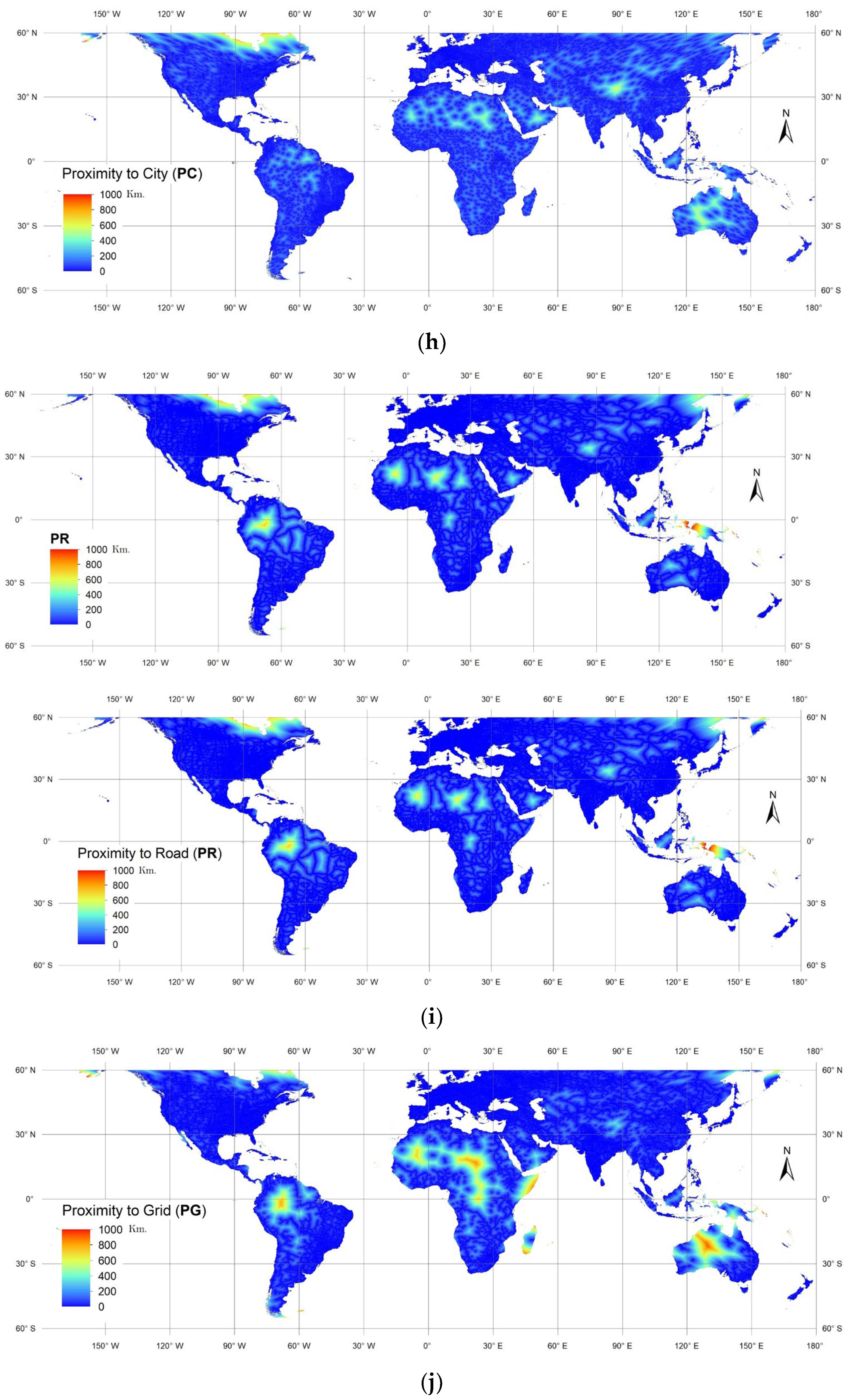
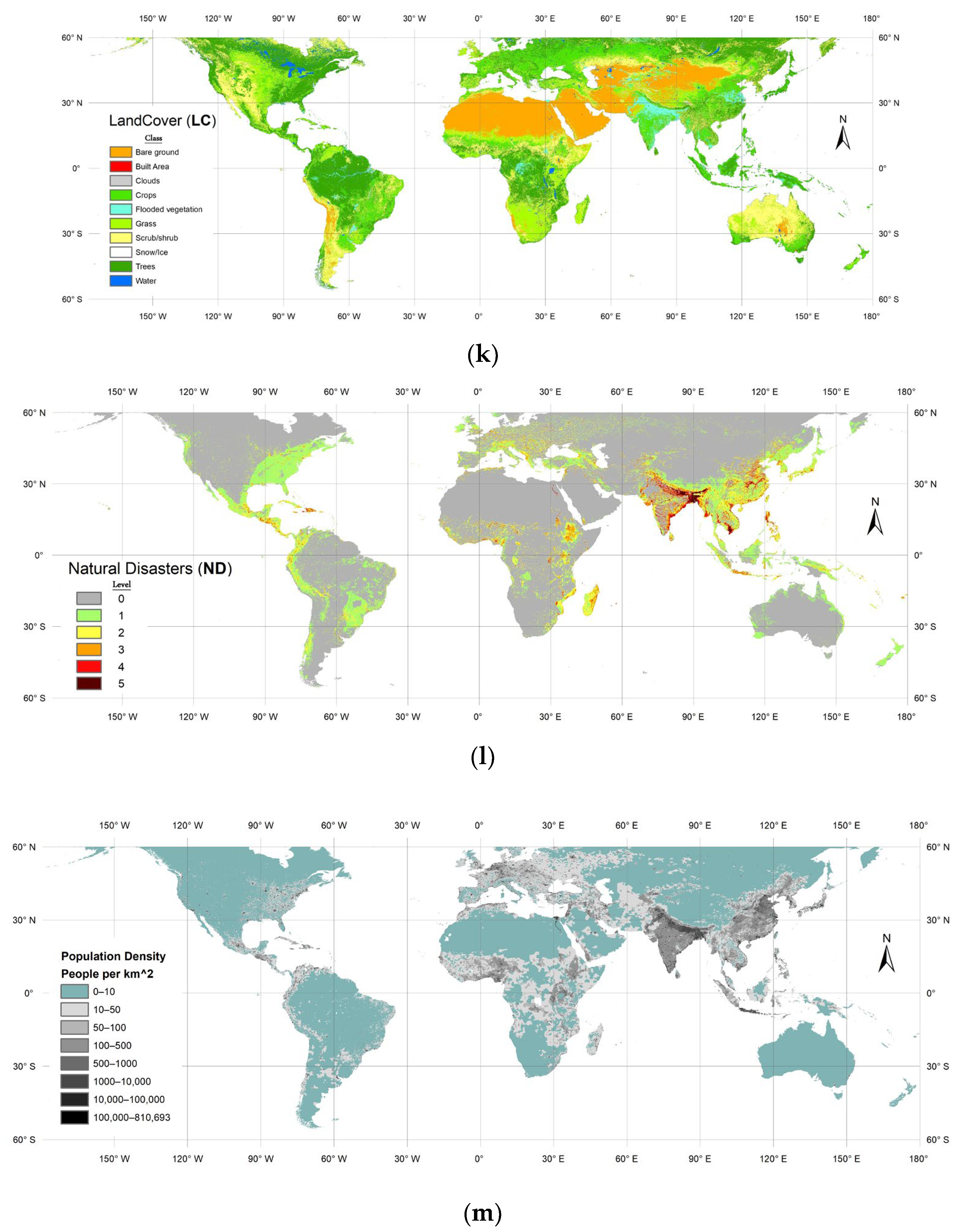
2.1.2. Conditioning Factors

Natural resource criteria, such as wind speed (WS) and solar radiation (SR), are key factors when choosing wind and solar farm locations [33]. However, other environmental and economic parameters are equally significant in the placement decision of RE systems [34]. Therefore, the most common factors that mimic the global scope of this study have been captured based on an extensive review of publications that addressed the site suitability assessment of wind and solar stations for different regions worldwide [1,5,6,7,12,20,35,36,37,38,39,40,41,42,43,44,45,46,47,48,49,50,51,52,53,54,55,56,57,58,59]. Accordingly, WS and Wind Density (WD) were considered technical factors for siting wind stations. However, they were replaced by SR, Air Temperature (AT) and Cloud Index (CI) when assessing the site suitability of solar farms. Moreover, eight other indicators participated in evaluating both types of energy, namely, Slope (S), Elevation (E), Landcover (LC), Proximity to Road (PR), Proximity to Grid (PG), Proximity to City (PC), Natural Disasters (ND) and Population Density (PD), which covered economic, environmental, and social aspects. For more details on the importance of these criteria, refer to the literature as they are comprehensively discussed [35,43,46,47,59,60,61].
As we investigate globally, publicly available online spatial databases from reliable sources were considered to collect global datasets for the criteria under consideration. WS and WD data at an altitude of 100 m were downloaded from the database of Global Wind Atlas v3.1 to meet the technical requirements of a modern wind turbine. For solar PV technologies, Global Solar Atlas v2.6 was used to gather the spatial datasets of AT and Global Horizontal Irradiation (GHI), which is the overall SR received at the horizontal surface on the ground [46]. Notably, the data of Global Wind Atlas and Global Solar Atlas, based on re-analyzed climate data, are widely used in formulating technical factors for siting RE plants [5,6,35]. In addition, CI factor data were acquired from the EarthEnv project database, which is based on 15 years of cloud observations derived from twice-daily MODIS satellite imagery [62]. Additionally, the digital elevation model products of SRTM 90m v4.1 available on the EarthEnv platform are certified to represent the E and S factors [63]. Meanwhile, vector data for the locations of cities, road networks, and electricity grids worldwide were gathered from a published dataset. Their quality is verified through comparison with high-resolution satellite images [64]. In a later step, the vector data are employed to formulate the PC, PR, and PG indicators. Table 1 presents LC, ND, and PD data sources and more details on the characteristics of the considered datasets.
The collected datasets are standardized in terms of geo-referencing, resampling, and workspace (onshore between latitude 60° N to 60° S). The vector datasets are converted to raster layers using the Euclidean distance tool. Finally, thematic layers for the conditioning factors are generated with an appropriate symbology, as shown in Figure 3.

2.1.3. Training Dataset Extraction

Based on the sample inventory (locations of wind and solar plants) and thematic layers of the criteria under consideration, two training datasets were generated. The first dataset was allocated for siting onshore wind farms, with 10 evaluation factors/independent variables: WS, WD, S, E, LC, PR, PG, PC, ND, and PD. On the contrary, the second dataset is employed to assess site suitability for solar farms against 11 influential factors/independent variables (i.e., RR, AT, CI, S, E, LC, PR, PG, PC, ND, and PD). As for dependent variables, solar samples were assigned as non-wind in the first dataset, whereas wind samples were designated as non-solar in the second dataset.

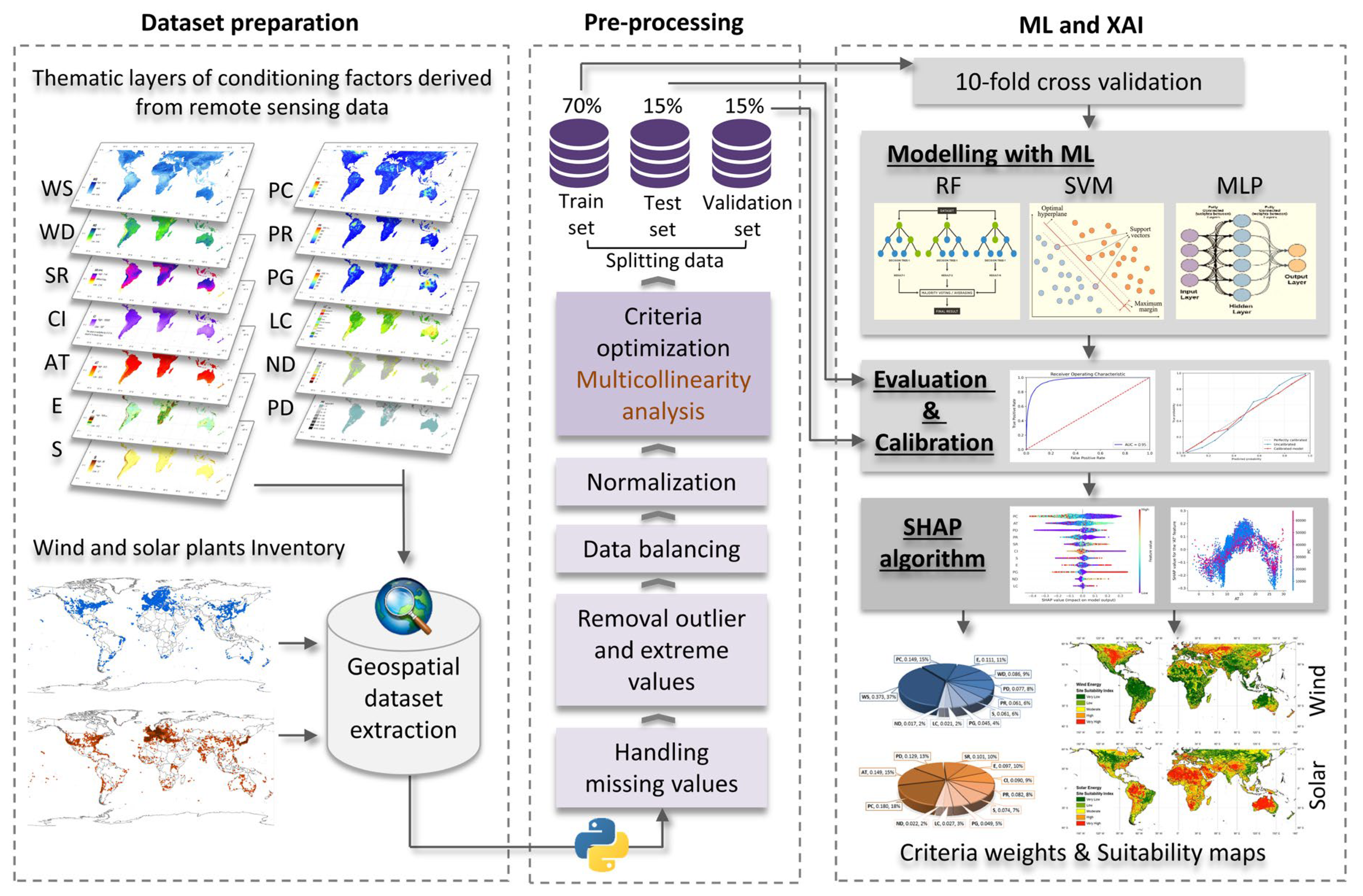
2.2. Dataset Pre-Processing

Ordinarily, real-world data can be incomplete (includes missing values), inaccurate (contains outlier and extreme values), and inconsistent [65]. Thus, preprocessing is an inevitable stage to clean, organize, and format the raw datasets, making them workable for ML models. In the present work, the two datasets mentioned earlier were preprocessed using the following successive steps:
  • Handling missing values: All missing values, whether for nominal or numeric attributes, are replaced by means and modes of the training data.
  • Removal outliers and extreme values: A filter is applied based on interquartile ranges to detect and remove outliers and extreme values that fall outside of what is expected.
  • Data balancing: For ML algorithms to operate unbiased, the number of samples must be balanced for each dependent variable [66]. To do so, our datasets were resampled by applying the Synthetic Minority Oversampling TEchnique (SMOTE), in which the minority samples are duplicated based on the minority data population.
  • Normalization: As data units of the independent variables vary widely, feature scaling or normalization is essential for objective functions of ML models to work correctly [67]. Accordingly, all attribute values under consideration were normalized on a standardized scale from 0 to 1.
  • Splitting data: An effective technique for understanding the performance of ML models is to divide the dataset into a training, validation, and testing set. Consistent with previous work [16,22,31], our dataset is split into 70% train set, 15% validation set, and 15% test set. In the training process, the training set is resampled to isolate the validation subset using a 10-fold cross-validation approach. The training and validation subset contributes to tuning the model parameters, whereas the test set is dedicated to evaluating the trained model accuracy.

Multicollinearity Analysis

As redundant independent variables are present, the calculations of ML algorithms are heavier and more time-consuming and even have lower performance [68]. Moreover, the multicollinearity between the parameters will affect the accuracy of the training results [69]. Therefore, multicollinearity analysis is a vital procedure to address these issues. To this end, a linear regression analysis was performed in which the square value of the correlation coefficient (R2) was calculated via SPSS software. Then, the R2 was utilized to compute the tolerance and variance inflation factor (VIF) for the input variables under consideration using Equations (1) and (2) [70]:
T i   =   1     R i 2 ,
VIF   =   1 T i .
The analysis indicates a multicollinearity issue between the considered criteria if T is less than 0.1 and/or VIF is larger than 10 [71]. Thus, the design of the criteria system should be reconsidered.

2.3. ML-Based Modeling

ML models, which have the ability to learn from large datasets, seek to perform a specific task efficiently without using explicit instructions [72]. ML uses two types of techniques: supervised learning to tackle classification and regression issues and unsupervised learning to solve clustering problems [15]. Supervised learning algorithms have demonstrated their ability to handle complexity and nonlinearity in many site-suitability and susceptibility analyses [68]. In this study, three supervised algorithms (RF, SVM, and MLP) using Python programming language with the Scikit-Learn package (http://scikit-learn.org, accessed on 15 March 2022) are exploited to classify the site suitability of wind and solar plants on a global scale. The Python programming code is provided in the Supplementary Material.

2.3.1. Algorithms Implemented

RF is one of the most widely used models for classification and regression issues because of its simplicity, accuracy, and flexibility. The RF algorithm, an upgraded version of the decision tree approach, combines numerous decision trees into a single structure termed a forest [15,73]. With more trees, the forest becomes robust against noise, overfitting, and non-correlated attributes [18]. Therefore, the number and depth of trees need to be carefully specified to run the RF algorithm efficiently [31].
SVM is a powerful ML algorithm that applies the structural risk reduction concept and is built on the theoretical basis of statistical learning [74]. The SVM model has the ability to overcome any complex nonlinear relationship by using kernel functions that convert input data into high-dimensional feature space [15]. Organized procedures for defining parameters in the SVM algorithm are critical, as they determine the model’s performance accuracy [75].
MLP is a class of feed-forward artificial neural networks that uses the backpropagation algorithm for supervised training [76]. The neural networks of MLP are built up of three major structures: input, hidden and output layers. One layer of input nodes is assigned to receive the relevant decision factors, and another one is to output the classified results. On the contrary, one or more intermediate hidden layers are dedicated as a computational engine for the MLP algorithm [16,77].
The hyper-parameters of the above-mentioned algorithms (i.e., RF, SVM and MLP) are fine-tuned to achieve maximum classification accuracy. The best number of trees to run the RF classifier was 100, with a maximum depth of five along with other default settings of the Scikit-Learn package [78]. For the SVM model, the Radial Basis Function (RBF) was the best kernel type with C and gamma values of 0.1 and 0.001, respectively. Finally, the MLP accuracy has stabilized with 4 hidden layers, 0.1 learning rate, and 10 epochs.

2.3.2. Algorithm Performance Evaluation

Performance appraisal is a crucial part of modeling in which the accuracy of prediction maps is tested using a real-world dataset that the models have not seen before [79]. In this study, a confusion matrix is considered to derive classifiers’ performance metrics, namely, Sensitivity ( Se ), Specificity ( Sp ), overall accuracy ( P o ), kappa coefficient ( k * ), and the Area Under the Curve (AUC). Se and Sp are executed to assess the model’s ability to correctly recognize the presence and absence of RE farms, respectively [31,75]. P o and k * were used to evaluate the classification accuracy of our models as kappa, in particular, has the capability to rule out a correct prediction occurring by chance [17]. The aforementioned metrics can be better described as follows:
Se   =   TP TP + FN ,
Sp   =   TN TN + FP ,
P o   =   TP + TN ( TP + FP + TN + FN ) ,
P e   =   [ ( TP + FP ) ( TP + FN ) + ( FN + TN ) ( FP + TN ) ] ( TP + FP + TN + FN ) 2 ,
k *   =   P o P e 1 P e .
where TP is the true positive instances of the predicted positive class; FP is the false positive instances of the predicted positive class; TN is the true negative instances of the predicted negative class, and FN is the false negative instances of the predicted negative class [18]. P o also indicates the observed accuracy, whereas P e is the expected accuracy.
Ultimately, the AUC, denoting the area under the Receiver Operating Characteristic (ROC) curve, is considered owing to its ability to distinguish binary classifications [75]. The ROC curve is plotted on a biaxial graphic. The x-axis indicates the false positive rate, and the y-axis denotes the true positive rate. The area under the ROC curve ranges from 0.5 to 1, with the highest AUC stating the most effective model [68,79].

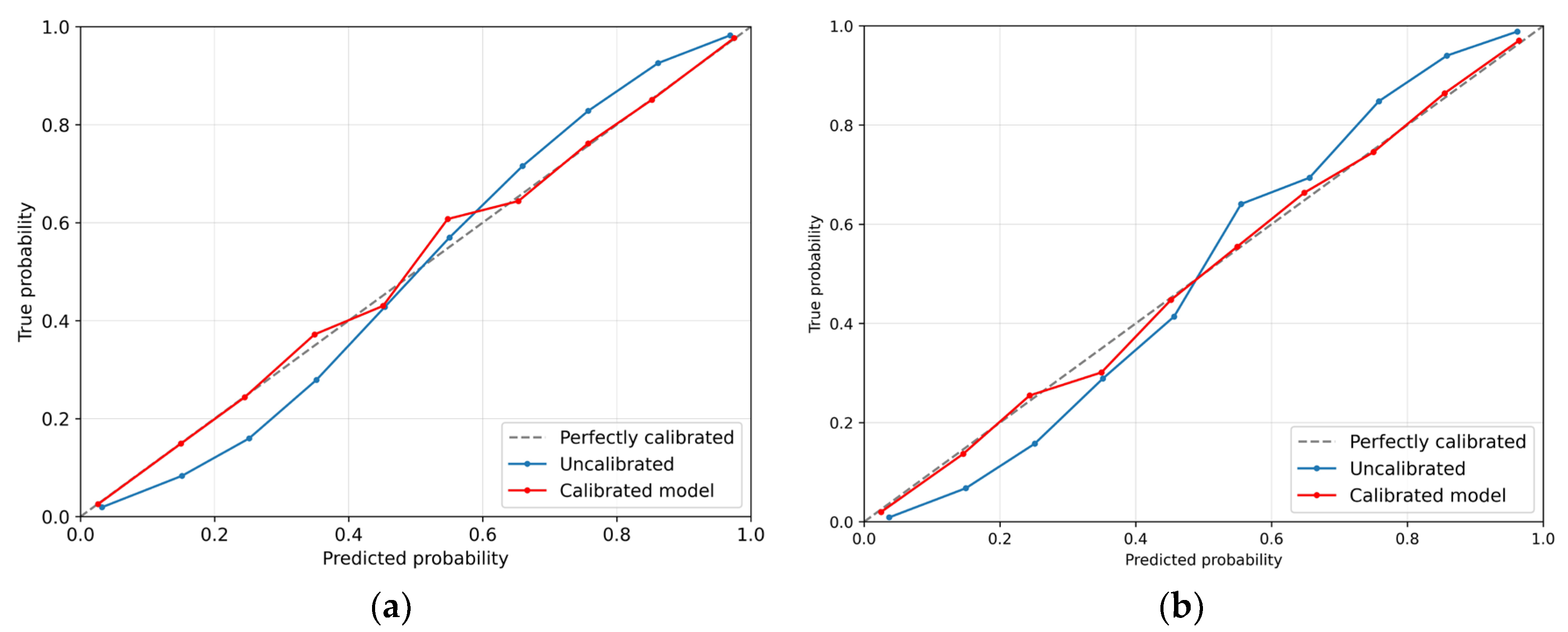
2.3.3. Model Calibration

Calibration is vital in training ML models that aim to convert model predictions into posterior class probabilities [80]. In other words, calibration works to approximate the predicted probabilities to the actual probabilities and thus obtain predictions that are more compatible with the real world [81]. The creation of a calibration plot (also known as a reliability plot) is the most common way to test the models’ calibration. Such a plot reveals any differences between the model’s predicted probability (x-axis) and the empirical probability in the data (y-axis) [82]. The closer the drawing curve is to the diagonal line, the better the calibration. As a popular method for calibrating models, isotonic regression is applied in this study. It is a non-parametric calibration method for binary classifiers in which the calibrated predictions are generated using an isotonic mapping transformation [81]. For more detail on the isotonic regression approach, the readers are referred to Leathart [83].

2.3.4. Explainable AI

XAI is a set of algorithms and plots that help humans understand and interpret the output of ML models [84]. XAI reveals the information that the actions are based on, thereby improving the performance of smart models. As the most popular XAI approach, the SHAP algorithm is performed in this work.
The SHAP algorithm was first developed by Shapley [85] to identify the contribution of individual players to the outcome of a cooperative team game [27]. Then, Lundberg et al. [86] recently introduced this concept to measure the participation and influence of parameters in formulating the outputs of ML models. The SHAP values estimate the magnitude and direction of each parameter contributing to the model’s output and present them in different kinds of interpretable plots [27]. The Shapley value is computed by taking the average of the marginal contribution across all conceivable parameter combinations, as described below [25]:
i   =   S N { i } | S | ! ( n | S | 1 ) ! n ! [ v ( S U { i } ) v ( S ) ] ,
where i is the contribution of parameter i; N is the set of all the parameters; n is the number of parameters in N; S is the subset of N which does not contain parameter i, and v (N) is the base value indicating the predicted result for each parameter in N without knowing the parameter values [28].
The SHAP index is usually estimated in various ways, such as Tree SHAP, Deep SHAP, and Kernel SHAP. This study employs Tree SHAP, a form of SHAP designed for tree-based ML models (e.g., decision trees, RF, XGBoost, and CatBoost) [87]. The Tree SHAP considers tree-based models to generate SHAP values in a matrix of equal size to the input dataset [88]. The SHAP values can determine whether the contribution of each input parameter is positive or negative. In this scenario, the SHAP analysis facilitates the understanding and identification of features most influential in predicting optimal sites for RE installations.
In this study, the Shapley explainer was adopted to obtain global and local interpretations of the ML model. The global explanation aims to estimate the general contribution of each conditioning factor in mapping the spatial suitability of wind and solar farms. The influence of factors is calculated as the mean of the absolute SHAP values throughout the entire dataset [29]. The local explanation, from another aspect, highlights the factors that made a significant contribution to the prediction by enabling us to identify the effect of each factor on classifying the individual pixels in the suitability map [25,29]. This capability gives us a deeper understanding of the model and the dataset. The global and local importance of the factors can be represented using the SHAP summary plot and the SHAP force plot, respectively.

3. Results

3.1. Collinearity of Conditioning Factors

A multicollinearity analysis was performed to achieve high predictive reliability and not overburden the trained models with extra parameters. The analysis results revealed that all criteria used in both datasets of this study yielded VIF values below 10 and T values exceeding 0.1, as presented in Table 2. The collinearity outcomes indicate that no strong correlation exists among the factors. Thus, the conditioning factors (independent variables) were all fed to the algorithms under consideration to derive their global weights and map the site’s suitability for wind and solar plants.

3.2. Evaluation and Calibration Results

Performance evaluation results using the 30% testing dataset demonstrated that the three algorithms have promising capabilities for predicting the spatial suitability to host wind and solar plants. Table 3 presents the appraisal of RF, SVM and MLP against Se , Sp , P o , k * and AUC metrics. Comparatively, the RF model was the most sensitive and specific in classifying the geospatial dataset of wind farms followed by the MLP and SVM, where the Se and Sp values were (0.88, 0.91), (0.79, 0.81), and (0.70, 0.75), respectively. A similar ordering was recorded within the solar dataset, revealing the ability of the RF model to correctly detect the presence and absence of wind and solar power plants. The highest overall accuracy in predicting suitable locations for wind and solar plants was when using the RF classifier (90% and 89%, respectively), followed by the MLP classifier (80% and 73%, respectively). By contrast, the SVM classifier provided the lowest P o (74% and 72%, respectively). Statistically, k * indices for the wind and solar modeling using the RF algorithm (0.79 and 0.78, respectively) were high compared with those using other algorithms under consideration. This result indicates substantial agreements between the model output and the ground truth. In addition, RF performance in wind and solar modeling had the best accuracy across the AUC metric (0.96 and 0.95, respectively), tracked by MLP and SVM. This finding implies no sign of overfitting in the RF model. Figure 4 displays the AUC plot of the RF model in which the ROC curves approach the upper left corner of the plot. This case is interpreted to mean that the AUC is closer to 1, and the overall accuracy is higher [16].
According to the aforementioned comparisons, the RF classifier achieved the highest accuracy within all performance metrics considered. Its merits include the ability to handle nonlinear relationships and low bias [18,89]. Therefore, the RF algorithm can be recommended as the best algorithm to predict the site’s suitability for wind and solar energy installations.
RF models were calibrated to obtain predictions compatible with real-world events. Figure 5a,b presents calibration plots for modeling the spatial suitability of wind and solar plants, respectively. The test calibration curve (the blue line) has an S-curve shape that is parallel to the perfect calibration line (diagonal gray line) in the wind and solar model of the RF classifier. However, the calibration of the models using the isotonic regression method (red line) significantly improved the predictive performance.

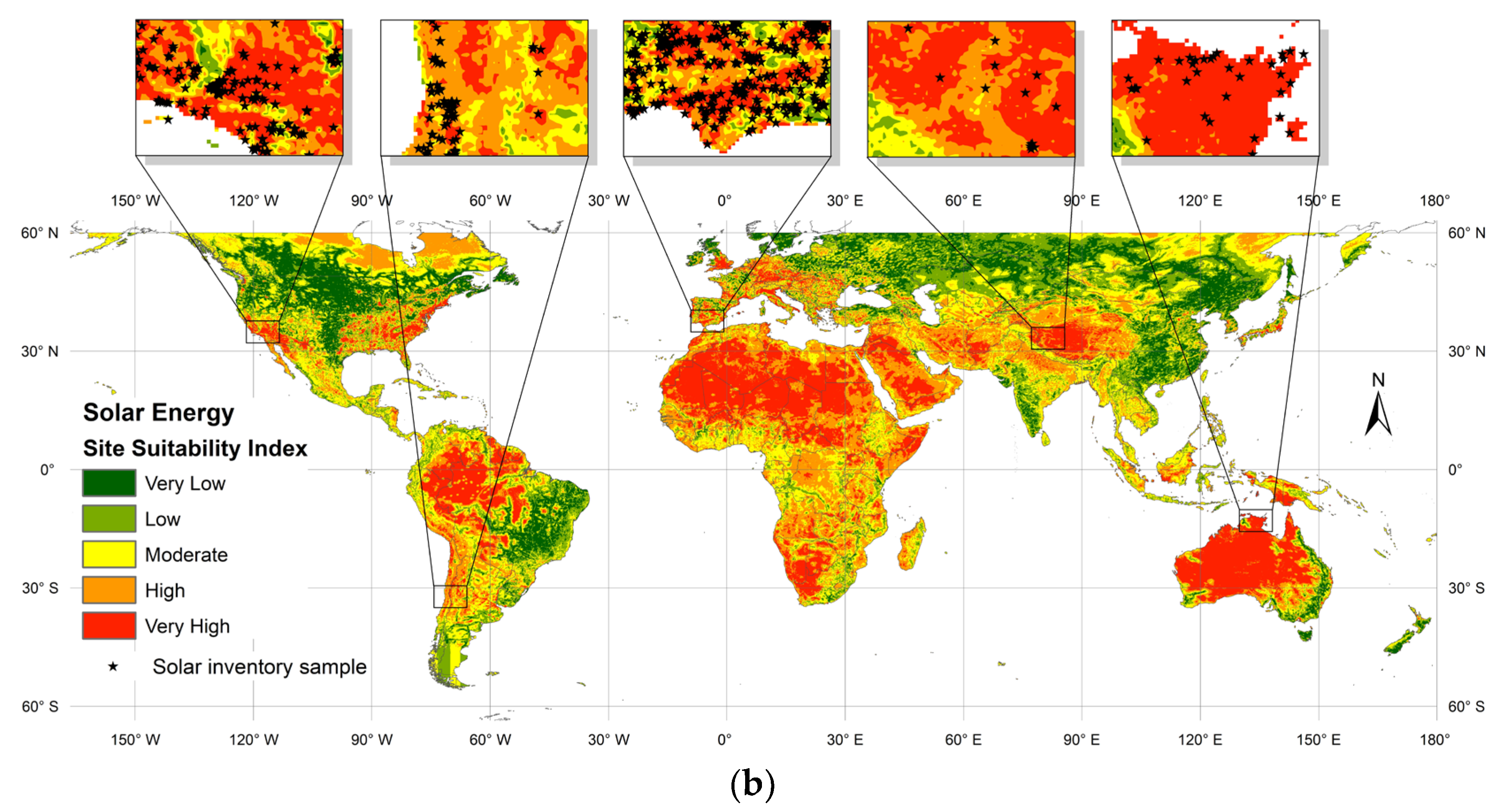
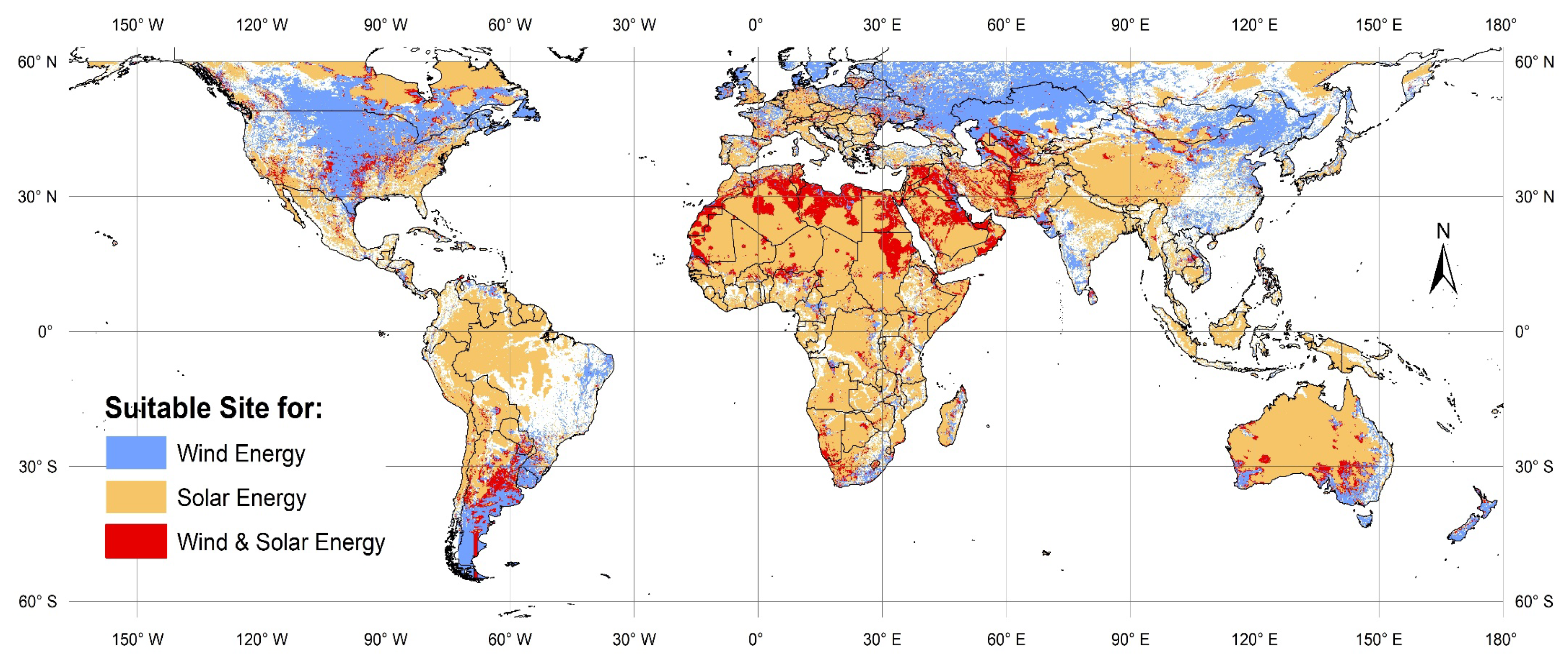
3.3. Global Suitability Mapping

RF was selected for further processing to generate spatial suitability maps to identify potential locations worldwide for the deployment of wind and solar energy equipment. The suitability maps were generated with a spatial resolution of 10 km. In each map, the degree of suitability is categorized into five classes using the equal interval classification method: very low (0.0–0.2), low (0.2–0.4), moderate (0.4–0.6), high (0.6–0.8), and very high (0.8–1.0). Figure 6 shows the results of the site suitability maps for wind and solar power plants.
The quantitative analysis in Table 4 shows that, for the wind map, the high and very high suitability categories cover 23.2% (~26.84 million km2) of the land, concentrated in regions above 30° in the Northern Hemisphere and below 30° in the Southern Hemisphere. America, Argentina, Russia, Kazakhstan and China are among the countries that have revealed significant areas of red and orange suitability indexes. Meanwhile, the moderate class (17.3%) is scattered across the site suitability map of wind energy, whereas 60% of the world’s considered area is low to very low for wind turbine deployment. As for the global map for hosting solar power plants, the high and very high suitability scores (24.0% and 19.4%, respectively) were more encouraging, covering a vast area of land, ~50.31 million km2. Territories on both sides of the equator, such as Africa, northern Latin America, northern Australia and parts of the Middle East and southern Asia, are considered the most suitable for the cultivation of solar PV panels. In addition, the very low class recorded a relatively small percentage of the area at 13.8%, followed by the low class with 18.9%, which constitutes a total of ~37.84 million km2 of land to be excluded from the planning of solar projects.
Overall, an opposite behavior is observed for the distribution of the suitability categories across the wind and solar energy maps. This discrepancy is because of the different spatial patterns of natural resource factors considered in this study, such as WS and SR. However, noteworthy regions of the planet can be found with promising suitability for both types of energy, as discussed in the next section.

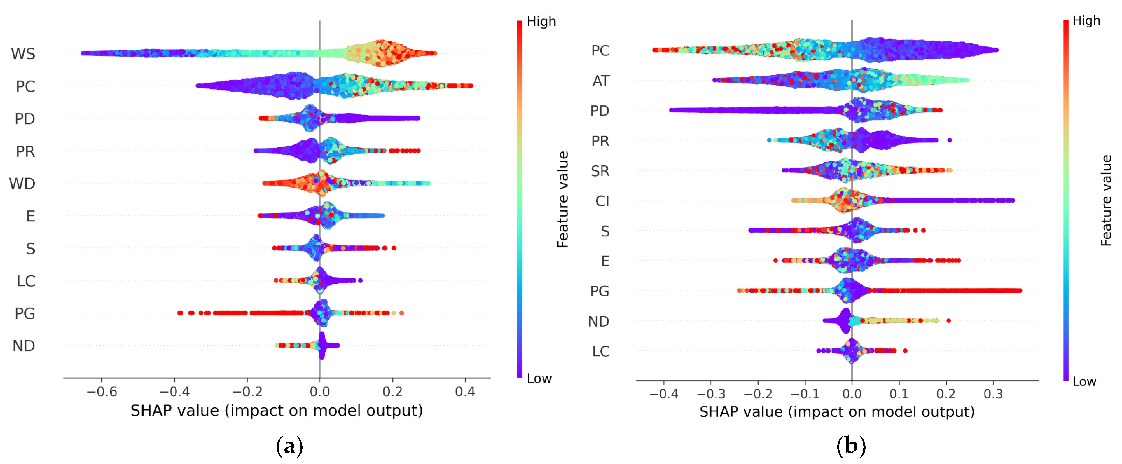
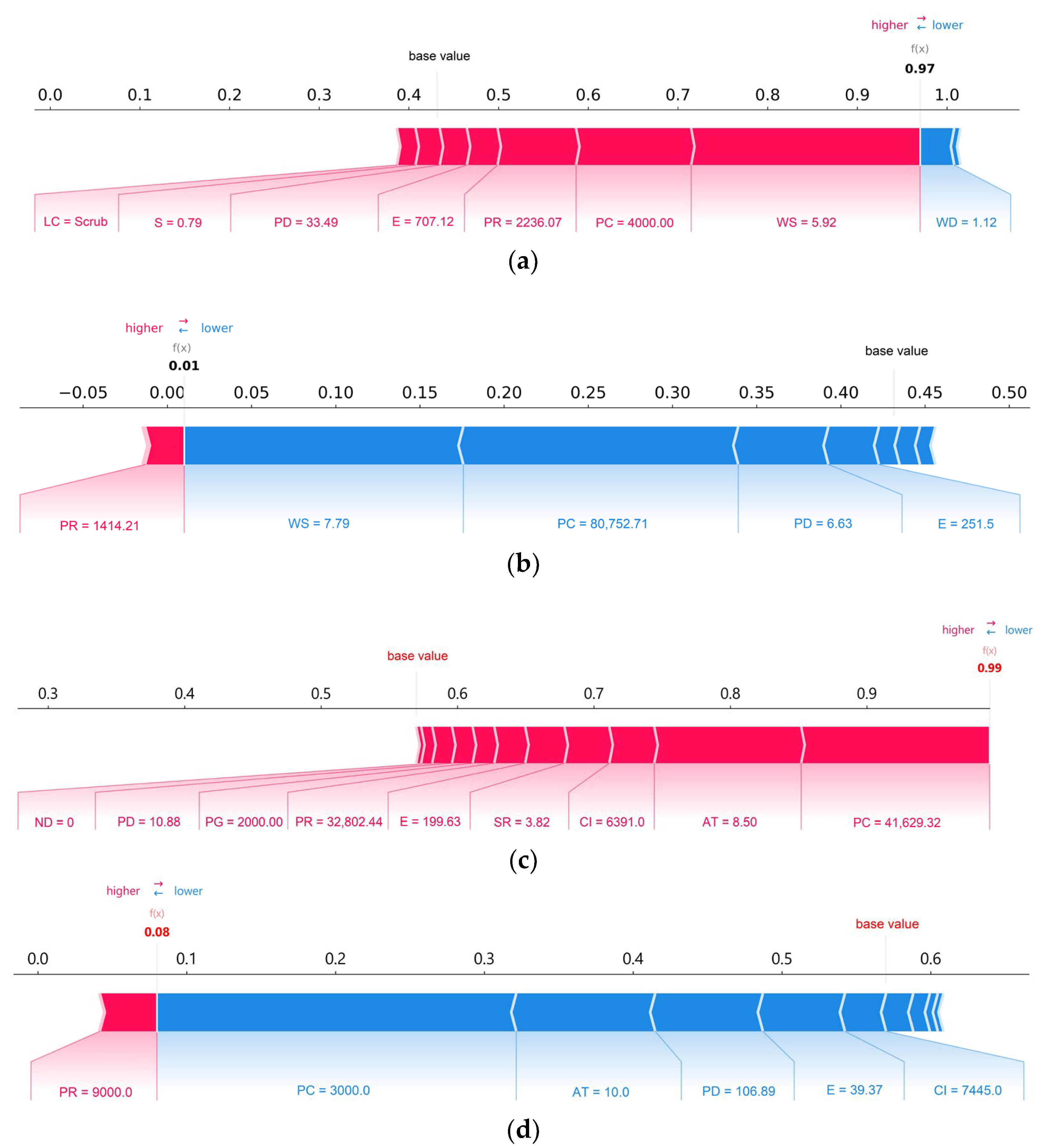
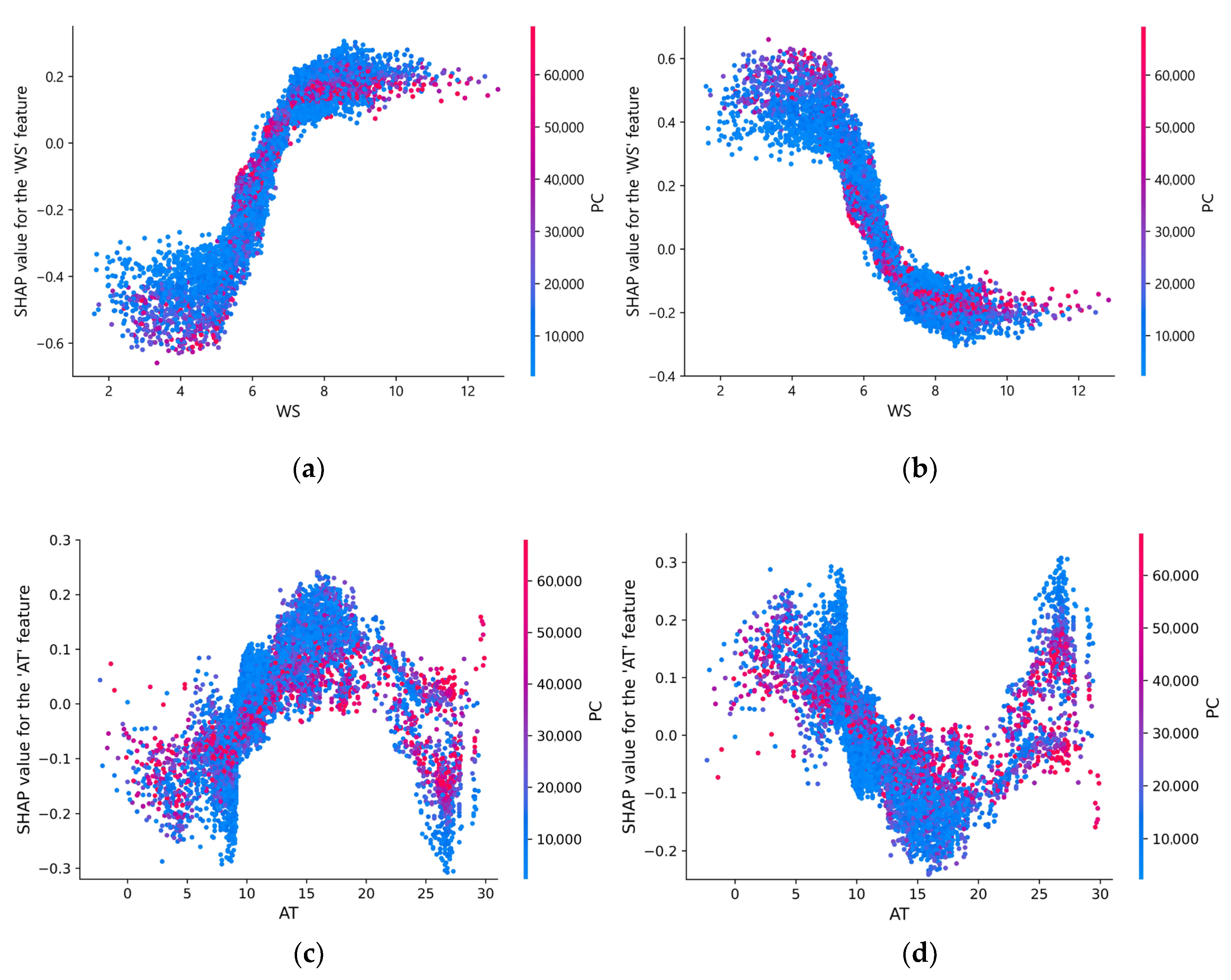
3.4. Predictive Model Explanation

The SHAP technique was applied to better understand the contribution of factors and their dependencies in formulating the prediction output. Shapley’s explanations are presented graphically in this section, globally and locally.
Globally, the impact of factors on the prediction output was investigated using the Shapley summary plot, as shown in Figure 7. The x-axis presents the SHAP value. A positive value implies an impact on the forward direction, whereas a negative one implies an impact on the backward direction toward attaining prediction outcomes. The y-axis ranks the factors in the order of significance. Each dot represents an observation from the original dataset. The value of each observation is displayed on the color scale ranging from low to high. Figure 7a shows that WS and PC have the greatest impact on the classification of the spatial suitability map for onshore wind systems. Taking an in-depth look, the concentration of red dots to the right of the baseline denotes that the high observation values of these factors increase the site’s potential to host wind turbines. In other words, the most suitable locations for siting wind plants are those with high WSs and a great distance from cities. From another aspect, PC and AT ranked first and second, respectively, in interpreting the influence of parameters involved in mapping site suitability for solar systems, as shown in Figure 7b. The blue color for PC and the bluish-green color for AT to the right of the baseline explain that places near cities and those with moderate temperatures are most likely to invest in solar PV energy. By contrast, PG, LC and ND had the least effect on the output of wind and solar models. Overall, the high impact of technical and economic factors can be recorded at the expense of other environmental and social factors.
Locally, a force plot was used to interpret the influence of factors on classifying certain pixels (Figure 8). The explanation shows how multiple factors interact to push the model’s output from the base value to the probability value of the initial prediction. As shown, the RF model can correctly classify pixels (a) and (c) with a 97% and 99% probability of being suitable for hosting wind and solar plants, respectively. By contrast, the model predicted pixels (b) and (d) to be spatially unsuitable for solar and wind systems with a probability of 1% and 8%, respectively. Each SHAP value is displayed by an arrow in the plot. Factors that increase the value of a positive classification (spatially suitable) are represented in red on the left, whereas those that decrease the value of a negative classification (spatially unsuitable) are indicated in blue on the right. In Figure 8a, for instance, WS, PC and PR play a significant role in raising the positive prediction of wind systems, whereas WD lowers the negative prediction. Furthermore, the values of WS, PC and PD factors were a determining criterion in assigning pixel un-suitability, as illustrated in Figure 8b. From another aspect, Figure 8c,d highlights the significant contributions of PC and AT factors in classifying the suitability of the observations for solar farm development.
Figure 9 shows the dependence plots for further understanding the factors that have a significant or dynamic effect on the prediction output. Such plots demonstrate the SHAP value of the features against the feature value of all instances under consideration. In Figure 9a,b the interactions between the WS and PC are plotted for the spatially suitable and unsuitable classes of wind power installations, respectively. The actual values of the first factor (WS) are represented on the x-axis, whereas the left y-axis displays the SHAP value associated with the factor. Positive values indicate that the factors contribute positively to the classification and vice versa. The colors denote the SHAP values given to the second factor (PC). Figure 9a shows that SHAP values get larger with increasing WS and PC leading to a positive prediction of site suitability for wind systems. The dependency between these factors takes an opposite pattern in classifying the unsuitable classes, as shown in Figure 9b. As the most influential factors in classifying the spatial suitability of solar stations, the interaction between AT and PC was represented using the same graphical approach mentioned above. Figure 9c,d shows dependence plots to predict suitable and unsuitable pixels for PV solar panel deployment. These plots revealed that AT values between 10 °C and 20 °C with a smaller distance to cities control the SHAP values, thereby formulating the prediction results.

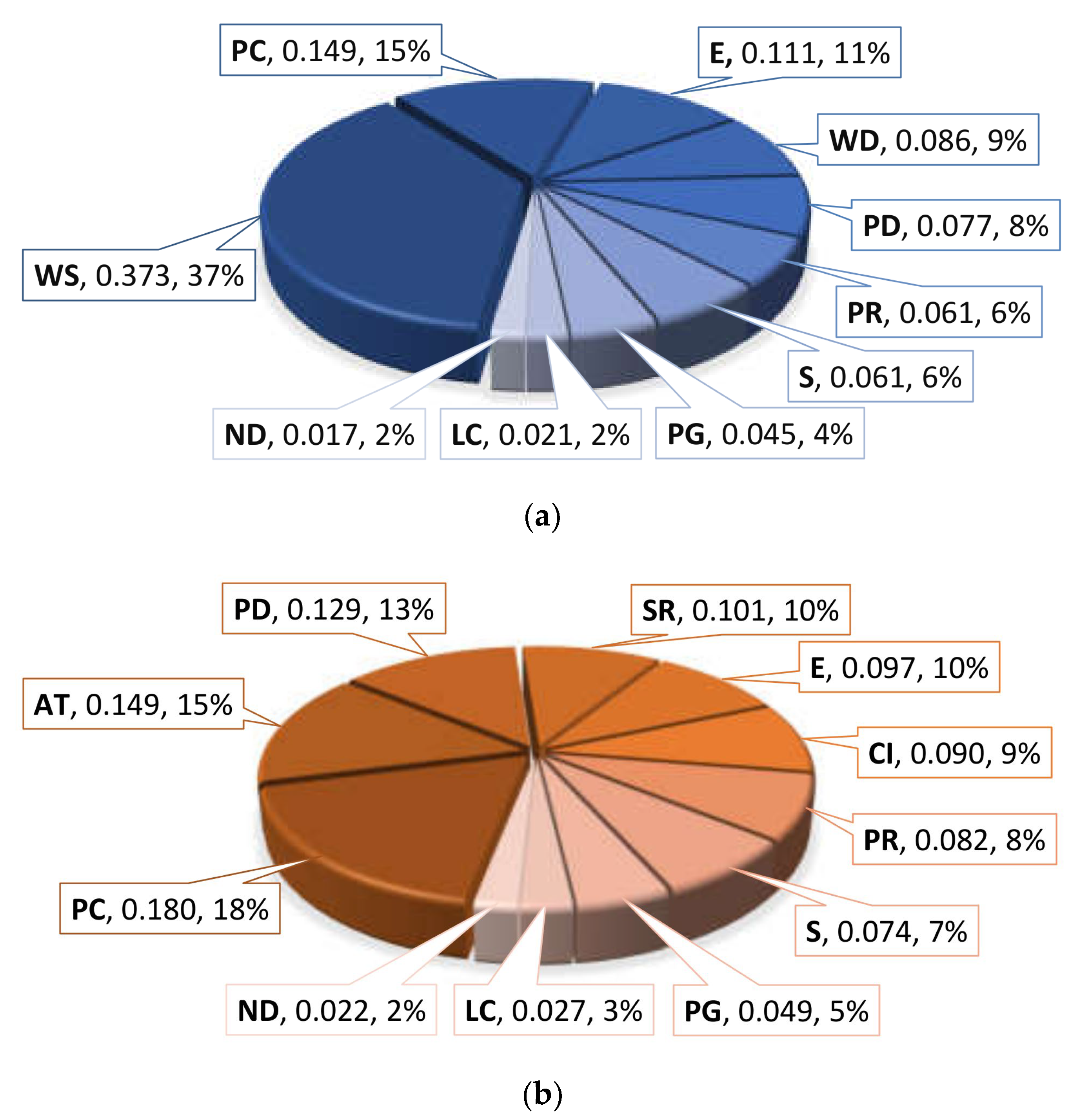
3.5. Weight of Conditioning Factors
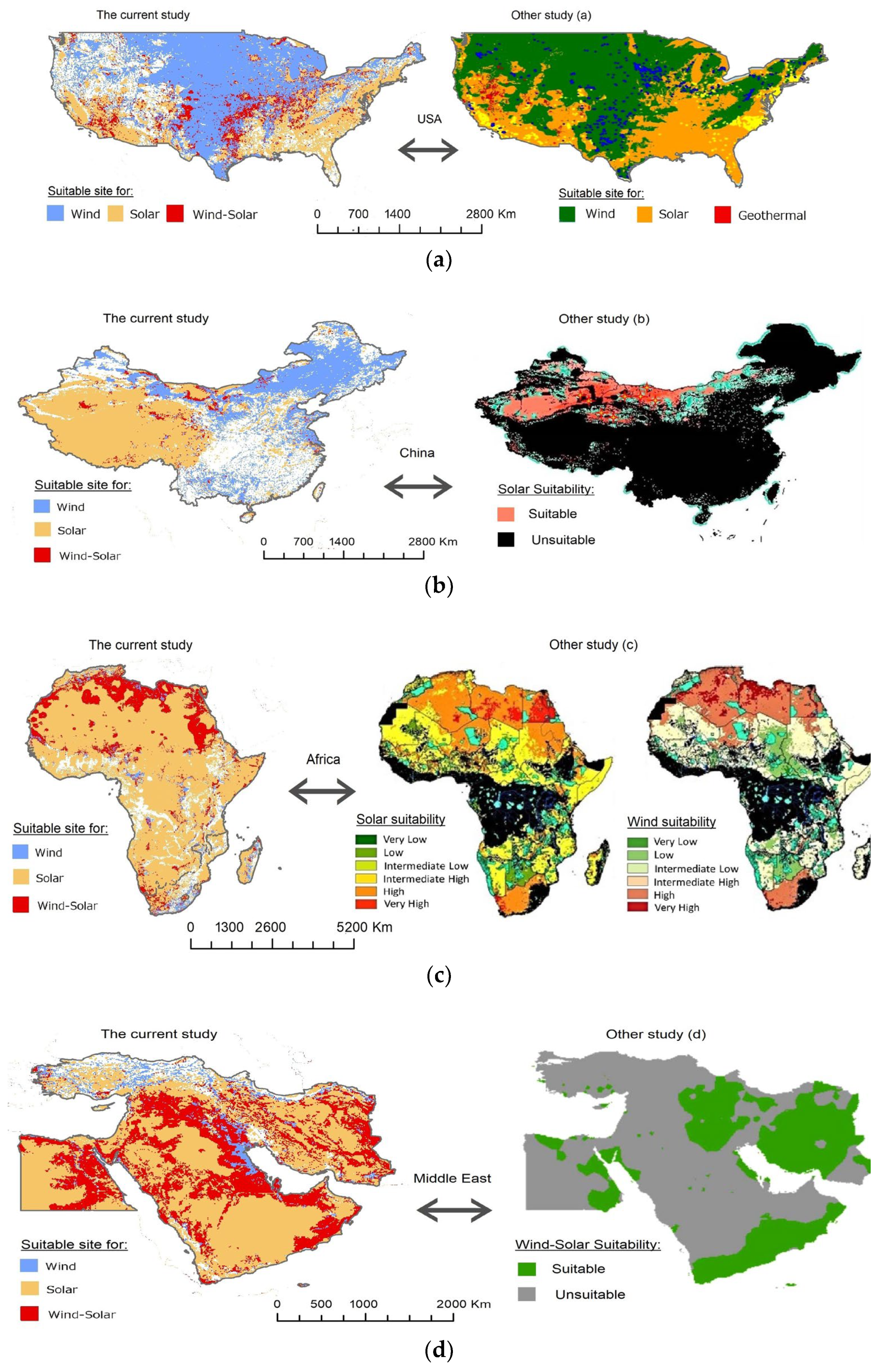
The relative weight of each conditioning factor within the RF algorithm-based modeling is calculated according to the mean decrease in impurity (MDI), sometimes called “gini importance” [90]. Figure 10 depicts the weights and contributions of each factor used in modeling and predicting land suitability for wind and solar power plants. Accordingly, the most influential parameter in the wind spatial modeling was WS (0.373), followed by PC (0.149). The E, WD and PD ranked the third, fourth and fifth with weights of 0.111, 0.086 and 0.077, respectively. Meanwhile, PR and S factors yielded an equal weight score of 0.061. Additionally, ND seemed to have no clear contribution to wind farm suitability mapping and was ranked 10th (0.017). In terms of the global suitability map of solar power plants, the weighting analysis for the dedicated factors exhibited the following ranking: PC (0.180), AT (0.149), PD (0.129), SR (0.101), E (0.097), CI (0.090), PR (0.082), S (0.074), PG (0.049), LC (0.027) and ND (0.027).

4. Discussion

Conventional assessments of site suitability for RE plants often involve challenges represented in designing a decision-making criteria system, identifying the criteria weights and mapping the relevant suitability. However, the availability of real-world spatial data for wind and solar power systems along with RS datasets for critical conditioning factors has led to the formulation of more mature and less-biased ML-based solutions. The performance appraisal metrics considered in this study provide scientific evidence of the robustness of the RF, SVM and MLP algorithms in predicting optimal sites for hosting wind and solar farms. Although the three models achieved an overall accuracy of over 70%, the RF performed satisfactorily in the wind and solar modeling with P o values of 90% and 89%, respectively. The best k * and AUC result was found using the RF classifier, followed by MLP and SVM. Evidently, the RF algorithm is the most proper and stable algorithm for predicting land suitability classes for deploying green energy equipment. This result is consistent with the findings of previous work that demonstrated the efficient performance of the RF algorithm [15,18,22]. Meanwhile, the parameter importance analysis by the RF method revealed significant weight ratios for WS (37%), PC (15%), E (11%), and WD (9%) in mapping site suitability for wind farms. On the contrary, the parameters PC (18%), AT (15%), PD (13%), and SR (10%) had the greatest influence on the optimum site selection for wind stations. These weights indicate that technical and economic factors dominate the choice of location and are in line with the recommendations of many researchers [91,92,93,94].
The percentages of wind and solar plant inventory samples are analyzed based on individual suitability classes to evaluate the quality of site suitability maps produced by the RF model, as shown in Figure 11. Accordingly, more than 80% of the inventory samples fall under “high” and “very high” zones, indicating the validity of our suitability maps. Overall, 23.2% of the lands worldwide were mainly found within “high” and “very high” favorability for building wind power plants, whereas the proportion doubled to 43.4% for setting up solar energy farms. This result highlights the abundant technical and economic potential of our planet to invest in solar power compared with wind power. However, large-scale solar PV farms are the main cause of land degradation and habitat loss, among other clean energies [95].
For our results to be comparable with those of previous works, a standardized map of site suitability for wind, solar, and wind–solar plants is generated, as illustrated in Figure 12. In the overall map, regions with spatial suitability degrees for wind systems, between 0.5 and 1, are represented in cyan, making up 22.35% of the world’s land area. Similarly, the orange color indicates the available areas for investment in solar energy (47.48% of the world’s land) with a suitability score of more than 0.5. Places that fulfilled both conditions above are painted in red, covering 8.53% of the land, and are suitable for wind, solar and wind–solar hybrid plants. Our map also revealed that 21.64% of the studied land was unsuitable for any energy systems under consideration.
The current map (Figure 12) is in line with the results of previous studies that covered individual countries or regions, as highlighted in Figure 13. For example, the southeastern and southwestern regions of the United States showed their suitability for hosting solar farms, supporting the report of Shahab et al. [22]. In addition, western China have revealed promising areas for investment in solar energy. This result is consistent with the maps of related study conducted in this country [96]. Meanwhile, our findings are harmonic with the report of a recent study investigating the site suitability for wind and solar plants in the entire African continent [97]. We both stated that the whole continent has moderate to very high suitability for solar plants, whereas the northern countries were the most likely to deploy wind turbines alongside solar PV panels. Moreover, in the Middle East, the results were comparable with the recommendations of Jahangiri et al. [98].
These trends highlight the spatial policies of wind and solar energy development under various technical, economic, and environmental constraints. As the cost of investing in RE continues to drop, policymakers and stakeholders must carefully consider appropriate spatial opportunities to host wind-solar hybrid systems for stable energy supplies, reduced land consumption and climate change mitigation. In addition to mapping the spatial suitability of wind and solar plants globally, the current research work presents a set of potential practical applications. Micro investigations of wind and solar systems can be carried out with high spatial resolution (e.g., 1 km) for specific continents or countries using the proposed ML-based framework. In addition, the reported global weightings assist decision-makers, particularly in developing countries that lack real-world experiences of RE farms, in generating bias-free MCDM-based solutions with less time and effort.

5. Conclusions

In this study, three ML algorithms (i.e., RF, SVM, and MLP) were tested to perform a global site suitability assessment for wind and solar plants using 55,619 real-world samples and 13 conditioning factors. The investigation results indicated the superiority of the RF algorithm in all the performance metrics ( Se   = 0.88/0.91, Sp   = 0.91/0.88, P o   = 0.90/0.89, k *   = 0.79/0.78, and AUC = 0.96/0.95); thus, this algorithm can be suggested as a sensible model for mapping land suitability of wind and solar installations. The XAI-based importance analysis revealed a high influence of technical and economic criteria on spatial decision-making with the highest weights for locating wind farms (WS = 0.373, PC = 0.149, E = 0.111 and WD = 0.086) and solar farms (PC = 0.180, AT = 0.149, PD = 0.129 and SR = 0.101). The global maps of site suitability developed in this work highlight 22.35% and 47.48% of the world’s land as advisable for hosting onshore wind and solar power plants, respectively. Both types of energy can be deployed side by side on 8.53% of the studied planet area.
As a useful worldwide assessment, the study findings are a starting point for scholars to conduct more detailed investigations of the new opportunities announced. Furthermore, the current results could potentially stimulate stakeholders to create new cross-border investments in the RE sector. The present paper has limitations. The study focuses on exploring suitable regions for onshore wind and solar PV farms against only a set of common evaluation factors. For future screening, spatial suitability maps can be sifted based on the more restricted zone. Global spatial assessment of offshore wind and concentrated solar energy is another potential avenue for future research.

Supplementary Materials

The following supporting information can be downloaded at: https://www.mdpi.com/article/10.3390/ijgi11080422/s1.

Author Contributions

Conceptualization, Mourtadha Sarhan Sachit, Helmi Zulhaidi Mohd Shafri, Ahmad Fikri Abdullah, Azmin Shakrine Mohd Rafie and Mohamed Barakat A. Gibril; methodology, Mourtadha Sarhan Sachit and Helmi Zulhaidi Mohd Shafri; software, Mourtadha Sarhan Sachit and Mohamed Barakat A. Gibril; formal analysis, Mourtadha Sarhan Sachit, Ahmad Fikri Abdullah and Azmin Shakrine Mohd Rafie; validation, Mourtadha Sarhan Sachit and Helmi Zulhaidi Mohd Shafri; writing—original draft, Mourtadha Sarhan Sachit; writing—review and editing, Helmi Zulhaidi Mohd Shafri, Ahmad Fikri Abdullah and Azmin Shakrine Mohd Rafie; visualization, Mourtadha Sarhan Sachit and Mohamed Barakat A. Gibril. All authors have read and agreed to the published version of the manuscript.

Funding

This research received no external funding.

Data Availability Statement

Publicly available datasets were analyzed in this study. These data can be found in Table 1.

Acknowledgments

The authors acknowledge the facilities and support provided by Universiti Putra Malaysia (UPM). The anonymous reviewers’ comments in refining this manuscript are also greatly appreciated.

Conflicts of Interest

The authors declare no conflict of interest.

References

  1. Rediske, G.; Siluk, J.C.M.; Michels, L.; Rigo, P.D.; Rosa, C.B.; Cugler, G. Multi-Criteria Decision-Making Model for Assessment of Large Photovoltaic Farms in Brazil. Energy 2020, 197, 117167. [Google Scholar] [CrossRef]
  2. Li, M.; Virguez, E.; Shan, R.; Tian, J.; Gao, S.; Patiño-Echeverri, D. High-Resolution Data Shows China’s Wind and Solar Energy Resources Are Enough to Support a 2050 Decarbonized Electricity System. Appl. Energy 2022, 306, 117996. [Google Scholar] [CrossRef]
  3. Kapica, J.; Canales, F.A.; Jurasz, J. Global Atlas of Solar and Wind Resources Temporal Complementarity. Energy Convers. Manag. 2021, 246, 114692. [Google Scholar] [CrossRef]
  4. Adedeji, P.A.; Akinlabi, S.A.; Madushele, N.; Olatunji, O.O. Neuro-Fuzzy Resource Forecast in Site Suitability Assessment for Wind and Solar Energy: A Mini Review. J. Clean. Prod. 2020, 269, 122104. [Google Scholar] [CrossRef]
  5. Rogna, M. Land Use Policy A First-Phase Screening Method for Site Selection of Large-Scale Solar Plants with an Application to Italy. Land Use Policy 2020, 99, 104839. [Google Scholar] [CrossRef]
  6. Amjad, F.; Shah, L.A. Identification and Assessment of Sites for Solar Farms Development Using GIS and Density Based Clustering Technique—A Case of Pakistan. Renew. Energy 2020, 155, 761–769. [Google Scholar] [CrossRef]
  7. Barzehkar, M.; Parnell, K.E.; Mobarghaee Dinan, N.; Brodie, G. Decision Support Tools for Wind and Solar Farm Site Selection in Isfahan Province, Iran. Clean Technol. Environ. Policy 2020, 23, 1179–1195. [Google Scholar] [CrossRef]
  8. Elboshy, B.; Alwetaishi, M.; Aly, R.M.H.; Zalhaf, A.S. A Suitability Mapping for the PV Solar Farms in Egypt Based on GIS-AHP to Optimize Multi-Criteria Feasibility. Ain Shams Eng. J. 2022, 13, 101618. [Google Scholar] [CrossRef]
  9. Haddad, B.; Díaz-Cuevas, P.; Ferreira, P.; Djebli, A.; Pérez, J.P. Mapping Concentrated Solar Power Site Suitability in Algeria. Renew. Energy 2021, 168, 838–853. [Google Scholar] [CrossRef]
  10. Diemuodeke, E.O.; Addo, A.; Oko, C.O.C.; Mulugetta, Y.; Ojapah, M.M. Optimal Mapping of Hybrid Renewable Energy Systems for Locations Using Multi-Criteria Decision-Making Algorithm. Renew. Energy 2019, 134, 461–477. [Google Scholar] [CrossRef]
  11. Dhunny, A.Z.; Doorga, J.R.S.; Allam, Z.; Lollchund, M.R.; Boojhawon, R. Identification of Optimal Wind, Solar and Hybrid Wind-Solar Farming Sites Using Fuzzy Logic Modelling. Energy 2019, 188, 116056. [Google Scholar] [CrossRef]
  12. Feng, J. Wind Farm Site Selection from the Perspective of Sustainability: A Novel Satisfaction Degree-Based Fuzzy Axiomatic Design Approach. Int. J. Energy Res. 2021, 45, 1097–1127. [Google Scholar] [CrossRef]
  13. Gao, J.; Guo, F.; Ma, Z.; Huang, X. Multi-Criteria Decision-Making Framework for Large-Scale Rooftop Photovoltaic Project Site Selection Based on Intuitionistic Fuzzy Sets. Appl. Soft Comput. 2021, 102, 107098. [Google Scholar] [CrossRef]
  14. Zardari, N.H.; Ahmed, K.; Shirazi, S.M.; Yusop, Z. Bin Weighting Methods and Their Effects on Multi-Criteria Decision Making Model Outcomes in Water Resources Management; Springer: Cham, Switzerland, 2014; ISBN 978-3-319-12585-5. [Google Scholar]
  15. Al-ruzouq, R.; Shanableh, A.; Yilmaz, A.G.; Idris, A. Dam Site Suitability Mapping and Analysis Using an Integrated GIS and Machine Learning Approach. Water 2019, 11, 1880. [Google Scholar] [CrossRef] [Green Version]
  16. Almansi, K.Y.; Shariff, A.R.M.; Abdullah, A.F.; Ismail, S.N.S. Hospital Site Suitability Assessment Using Three Machine Learning Approaches: Evidence from the Gaza Strip in Palestine. Appl. Sci. 2021, 11, 11054. [Google Scholar] [CrossRef]
  17. Al-Ruzouq, R.; Abdallah, M.; Shanableh, A.; Alani, S.; Obaid, L.; Gibril, M.B.A. Waste to Energy Spatial Suitability Analysis Using Hybrid Multi-Criteria Machine Learning Approach. Environ. Sci. Pollut. Res. 2021, 29, 2613–2628. [Google Scholar] [CrossRef]
  18. Taghizadeh-Mehrjardi, R.; Nabiollahi, K.; Rasoli, L.; Kerry, R.; Scholten, T. Land Suitability Assessment and Agricultural Production Sustainability Using Machine Learning Models. Agronomy 2020, 10, 573. [Google Scholar] [CrossRef]
  19. Boogar, A.R.; Salehi, H.; Pourghasemi, H.R.; Blaschke, T. Predicting Habitat Suitability and Conserving Juniperus Spp. Habitat Using SVM and Maximum Entropy Machine Learning Techniques. Water 2019, 11, 2049. [Google Scholar] [CrossRef] [Green Version]
  20. Asadi, M.; Pourhossein, K. Neural Network-Based Modelling of Wind/Solar Farm Siting: A Case Study of East-Azerbaijan. Int. J. Sustain. Energy 2020, 40, 1–22. [Google Scholar] [CrossRef]
  21. Jani, H.K.; Kachhwaha, S.S.; Nagababu, G.; Das, A. Temporal and Spatial Simultaneity Assessment of Wind-Solar Energy Resources in India by Statistical Analysis and Machine Learning Clustering Approach. Energy 2022, 248, 123586. [Google Scholar] [CrossRef]
  22. Shahab, A.; Singh, M.P. Comparative Analysis of Different Machine Learning Algorithms in Classification of Suitability of Renewable Energy Resource. In Proceedings of the 2019 International Conference on Communication and Signal Processing (ICCSP), Melmaruvathur, India, 4–6 April 2019; pp. 360–364. [Google Scholar] [CrossRef]
  23. Chakraborty, D.; Başağaoğlu, H.; Winterle, J. Interpretable vs. Noninterpretable Machine Learning Models for Data-Driven Hydro-Climatological Process Modeling. Expert Syst. Appl. 2021, 170, 114498. [Google Scholar] [CrossRef]
  24. Adadi, A.; Berrada, M. Peeking Inside the Black-Box: A Survey on Explainable Artificial Intelligence (XAI). IEEE Access 2018, 6, 52138–52160. [Google Scholar] [CrossRef]
  25. Matin, S.S.; Pradhan, B. Earthquake-Induced Building-Damage Mapping Using Explainable Ai (Xai). Sensors 2021, 21, 4489. [Google Scholar] [CrossRef]
  26. Barredo Arrieta, A.; Díaz-Rodríguez, N.; Del Ser, J.; Bennetot, A.; Tabik, S.; Barbado, A.; Garcia, S.; Gil-Lopez, S.; Molina, D.; Benjamins, R.; et al. Explainable Artificial Intelligence (XAI): Concepts, Taxonomies, Opportunities and Challenges toward Responsible AI. Inf. Fusion 2020, 58, 82–115. [Google Scholar] [CrossRef] [Green Version]
  27. Dikshit, A.; Pradhan, B. Explainable AI in Drought Forecasting. Mach. Learn. Appl. 2021, 6, 100192. [Google Scholar] [CrossRef]
  28. Dikshit, A.; Pradhan, B. Interpretable and Explainable AI (XAI) Model for Spatial Drought Prediction. Sci. Total Environ. 2021, 801, 149797. [Google Scholar] [CrossRef] [PubMed]
  29. Collini, E.; Palesi, L.A.I.; Nesi, P.; Pantaleo, G.; Nocentini, N.; Rosi, A. Predicting and Understanding Landslide Events with Explainable AI. IEEE Access 2022, 10, 31175–31189. [Google Scholar] [CrossRef]
  30. Abdollahi, A.; Pradhan, B. Urban Vegetation Mapping from Aerial Imagery Using Explainable AI (XAI). Sensors 2021, 21, 4738. [Google Scholar] [CrossRef]
  31. Al-Abadi, A.M. Mapping Flood Susceptibility in an Arid Region of Southern Iraq Using Ensemble Machine Learning Classifiers: A Comparative Study. Arab. J. Geosci. 2018, 11, 218. [Google Scholar] [CrossRef]
  32. Dunnett, S.; Sorichetta, A.; Taylor, G.; Eigenbrod, F. Harmonised Global Datasets of Wind and Solar Farm Locations and Power. Sci. Data 2020, 7, 1–12. [Google Scholar] [CrossRef]
  33. Ali, S.; Taweekun, J.; Techato, K.; Waewsak, J.; Gyawali, S. GIS Based Site Suitability Assessment for Wind and Solar Farms in Songkhla, Thailand. Renew. Energy 2019, 132, 1360–1372. [Google Scholar] [CrossRef]
  34. Anwarzai, M.A.; Nagasaka, K. Utility-Scale Implementable Potential of Wind and Solar Energies for Afghanistan Using GIS Multi-Criteria Decision Analysis. Renew. Sustain. Energy Rev. 2017, 71, 150–160. [Google Scholar] [CrossRef]
  35. Mentis, D.; Siyal, S.H.; Korkovelos, A.; Howells, M. A Geospatial Assessment of the Techno-Economic Wind Power Potential in India Using Geographical Restrictions. Renew. Energy 2016, 97, 77–88. [Google Scholar] [CrossRef]
  36. Tercan, E.; Eymen, A.; Urfalı, T.; Saracoglu, B.O. A Sustainable Framework for Spatial Planning of Photovoltaic Solar Farms Using GIS and Multi-Criteria Assessment Approach in Central Anatolia, Turkey. Land Use Policy 2021, 102, 105272. [Google Scholar] [CrossRef]
  37. Kannan, D.; Moazzeni, S.; mostafayi Darmian, S.; Afrasiabi, A. A Hybrid Approach Based on MCDM Methods and Monte Carlo Simulation for Sustainable Evaluation of Potential Solar Sites in East of Iran. J. Clean. Prod. 2021, 279, 122368. [Google Scholar] [CrossRef]
  38. Finn, T.; McKenzie, P. A High-Resolution Suitability Index for Solar Farm Location in Complex Landscapes. Renew. Energy 2020, 158, 520–533. [Google Scholar] [CrossRef]
  39. Habib, S.M.; El-Raie Emam Suliman, A.; Al Nahry, A.H.; Abd El Rahman, E.N. Spatial Modeling for the Optimum Site Selection of Solar Photovoltaics Power Plant in the Northwest Coast of Egypt. Remote Sens. Appl. Soc. Environ. 2020, 18, 100313. [Google Scholar] [CrossRef]
  40. Ibrahim, G.R.F.; Hamid, A.A.; Darwesh, U.M.; Rasul, A. A GIS-Based Boolean Logic-Analytical Hierarchy Process for Solar Power Plant (Case Study: Erbil Governorate—Iraq). Environ. Dev. Sustain. 2020, 23, 6066–6083. [Google Scholar] [CrossRef]
  41. Mokarram, M.; Mokarram, M.J.; Gitizadeh, M.; Niknam, T.; Aghaei, J. A Novel Optimal Placing of Solar Farms Utilizing Multi-Criteria Decision-Making (MCDA) and Feature Selection. J. Clean. Prod. 2020, 261, 12109. [Google Scholar] [CrossRef]
  42. Hassaan, M.A.; Hassan, A.; Al-Dashti, H. GIS-Based Suitability Analysis for Siting Solar Power Plants in Kuwait. Egypt. J. Remote Sens. Space Sci. 2020, 24, 453–461. [Google Scholar] [CrossRef]
  43. Mohamed, S.A. Application of Geo-Spatial Analytical Hierarchy Process and Multi-Criteria Analysis for Site Suitability of the Desalination Solar Stations in Egypt. J. Afr. Earth Sci. 2020, 164, 103767. [Google Scholar] [CrossRef]
  44. Ruiz, H.S.; Sunarso, A.; Ibrahim-Bathis, K.; Murti, S.A.; Budiarto, I. GIS-AHP Multi Criteria Decision Analysis for the Optimal Location of Solar Energy Plants at Indonesia. Energy Rep. 2020, 6, 3249–3263. [Google Scholar] [CrossRef]
  45. Ghose, D.; Naskar, S.; Shabbiruddin; Sadeghzadeh, M.; Assad, M.E.H.; Nabipour, N. Siting High Solar Potential Areas Using Q-GIS in West Bengal, India. Sustain. Energy Technol. Assess. 2020, 42, 100864. [Google Scholar] [CrossRef]
  46. Sun, L.; Jiang, Y.; Guo, Q.; Ji, L.; Xie, Y.; Qiao, Q.; Huang, G.; Xiao, K. A GIS-Based Multi-Criteria Decision Making Method for the Potential Assessment and Suitable Sites Selection of PV and CSP Plants. Resour. Conserv. Recycl. 2020, 168, 105306. [Google Scholar] [CrossRef]
  47. Bertsiou, M.M.; Theochari, A.P.; Baltas, E. Multi-Criteria Analysis and Geographic Information Systems Methods for Wind Turbine Siting in a North Aegean Island. Energy Sci. Eng. 2020, 9, 4–18. [Google Scholar] [CrossRef]
  48. Moradi, S.; Yousefi, H.; Noorollahi, Y.; Rosso, D. Multi-Criteria Decision Support System for Wind Farm Site Selection and Sensitivity Analysis: Case Study of Alborz Province, Iran. Energy Strateg. Rev. 2020, 29, 100478. [Google Scholar] [CrossRef]
  49. Ahmadi, S.H.R.; Noorollahi, Y.; Ghanbari, S.; Ebrahimi, M.; Hosseini, H.; Foroozani, A.; Hajinezhad, A. Hybrid Fuzzy Decision Making Approach for Wind-Powered Pumped Storage Power Plant Site Selection: A Case Study. Sustain. Energy Technol. Assess. 2020, 42, 100838. [Google Scholar] [CrossRef]
  50. Xu, Y.; Li, Y.; Zheng, L.; Cui, L.; Li, S.; Li, W.; Cai, Y. Site Selection of Wind Farms Using GIS and Multi-Criteria Decision Making Method in Wafangdian, China. Energy 2020, 207, 118222. [Google Scholar] [CrossRef]
  51. Cunden, T.S.M.; Doorga, J.; Lollchund, M.R.; Rughooputh, S.D.D.V. Multi-Level Constraints Wind Farms Siting for a Complex Terrain in a Tropical Region Using MCDM Approach Coupled with GIS. Energy 2020, 211, 118533. [Google Scholar] [CrossRef]
  52. Tan, Q.; Wei, T.; Peng, W.; Yu, Z.; Wu, C. Comprehensive Evaluation Model of Wind Farm Site Selection Based on Ideal Matter Element and Grey Clustering. J. Clean. Prod. 2020, 272, 122658. [Google Scholar] [CrossRef]
  53. Obane, H.; Nagai, Y.; Asano, K. Assessing Land Use and Potential Conflict in Solar and Onshore Wind Energy in Japan. Renew. Energy 2020, 160, 842–851. [Google Scholar] [CrossRef]
  54. Álvarez-Alvarado, J.M.; Ríos-Moreno, J.G.; Ventura-Ramos, E.J.; Ronquillo-Lomeli, G.; Trejo-Perea, M. An Alternative Methodology to Evaluate Sites Using Climatology Criteria for Hosting Wind, Solar, and Hybrid Plants. Energy Sources Part A Recover. Util. Environ. Eff. 2020, 1, 1–18. [Google Scholar] [CrossRef]
  55. Ali, T.; Nahian, A.J.; Ma, H. A Hybrid Multi-Criteria Decision-Making Approach to Solve Renewable Energy Technology Selection Problem for Rohingya Refugees in Bangladesh. J. Clean. Prod. 2020, 273, 122967. [Google Scholar] [CrossRef]
  56. Achbab, E.; Rhinane, H.; Maanan, M.; Saifaoui, D. Developing and Applying a GIS-Fuzzy AHP Assisted Approach to Locating a Hybrid Renewable Energy System with High Potential: Case of Dakhla Region-Morocco. In Proceedings of the 2020 IEEE International Conference of Moroccan Geomatics, Casablanca, Morroco, 11–13 May 2020. [Google Scholar]
  57. Unal Cilek, M.; Guner, E.D.; Tekin, S. The Combination of Fuzzy Analytical Hierarchical Process and Maximum Entropy Methods for the Selection of Wind Farm Location. Environ. Sci. Pollut. Res. 2022, 2022, 1–16. [Google Scholar] [CrossRef]
  58. Rezaei, M.; Khalilpour, K.R.; Jahangiri, M. Multi-Criteria Location Identification for Wind/Solar Based Hydrogen Generation: The Case of Capital Cities of a Developing Country. Int. J. Hydrogen Energy 2020, 45, 33151–33168. [Google Scholar] [CrossRef]
  59. Sadeghi, M.; Karimi, M. GIS-Based Solar and Wind Turbine Site Selection Using Multi-Criteria Analysis: Case Study Tehran, Iran. In Proceedings of the International Archives of the Photogrammetry, Remote Sensing and Spatial Information Sciences—ISPRS Archives, Tehran, Iran, 7–10 October 2017. [Google Scholar]
  60. Al Garni, H.Z.; Awasthi, A. Solar PV Power Plants Site Selection: A Review. In Advances in Renewable Energies and Power Technologies; Yahyaoui, I., Ed.; Elsevier: Amsterdam, The Netherlands, 2018; ISBN 9780128132173. [Google Scholar]
  61. Shao, M.; Han, Z.; Sun, J.; Xiao, C.; Zhang, S.; Zhao, Y. A Review of Multi-Criteria Decision Making Applications for Renewable Energy Site Selection. Renew. Energy 2020, 157, 377–403. [Google Scholar] [CrossRef]
  62. Wilson, A.M.; Jetz, W. Remotely Sensed High-Resolution Global Cloud Dynamics for Predicting Ecosystem and Biodiversity Distributions. PLoS Biol. 2016, 14, e1002415. [Google Scholar] [CrossRef] [PubMed]
  63. Amatulli, G.; Domisch, S.; Tuanmu, M.N.; Parmentier, B.; Ranipeta, A.; Malczyk, J.; Jetz, W. Data Descriptor: A Suite of Global, Cross-Scale Topographic Variables for Environmental and Biodiversity Modeling. Sci. Data 2018, 5, 180040. [Google Scholar] [CrossRef] [Green Version]
  64. Arderne, C.; NIcolas, C.; Zorn, C.; Koks, E.E. Data from: Predictive Mapping of the Global Power System Using Open Data. Nat. Sci. Data 2020, 7, 1–12. [Google Scholar] [CrossRef]
  65. Gonzalez Zelaya, C.V. Towards Explaining the Effects of Data Preprocessing on Machine Learning. Proc. Int. Conf. Data Eng. 2019, 2019, 2086–2090. [Google Scholar] [CrossRef]
  66. Islam, S.; Sara, U.; Rahman, A.; Kundu, D.; Hasan, M.; Kawsar, A.; Dipta, D.D.; Rezaul Karim, A.N.M. SGBBA: An Efficient Method for Prediction System in Machine Learning Using Imbalance Dataset. Int. J. Adv. Comput. Sci. Appl. 2021, 12, 430–441. [Google Scholar] [CrossRef]
  67. Liang, Z.; Liu, N. Efficient Feature Scaling for Support Vector Machines with a Quadratic Kernel. Neural Process. Lett. 2014, 39, 235–246. [Google Scholar] [CrossRef]
  68. Kalantar, B.; Ueda, N.; Saeidi, V.; Janizadeh, S.; Shabani, F.; Ahmadi, K.; Shabani, F. Deep Neural Network Utilizing Remote Sensing Datasets for Flood Hazard Susceptibility Mapping in Brisbane, Australia. Remote Sens. 2021, 13, 2638. [Google Scholar] [CrossRef]
  69. Katrutsa, A.; Strijov, V. Comprehensive Study of Feature Selection Methods to Solve Multicollinearity Problem According to Evaluation Criteria. Expert Syst. Appl. 2017, 76, 1–11. [Google Scholar] [CrossRef]
  70. Meng, F.; Liang, X.; Xiao, C.; Wang, G. Integration of GIS, Improved Entropy and Improved Catastrophe Methods for Evaluating Suitable Locations for Well Drilling in Arid and Semi-Arid Plains. Ecol. Indic. 2021, 131, 108124. [Google Scholar] [CrossRef]
  71. Saha, S. Groundwater Potential Mapping Using Analytical Hierarchical Process: A Study on Md. Bazar Block of Birbhum District, West Bengal. Spat. Inf. Res. 2017, 25, 615–626. [Google Scholar] [CrossRef]
  72. Han, S.; Jia, X.; Chen, X.; Gupta, S.; Kumar, A.; Lin, Z. Search Well and Be Wise: A Machine Learning Approach to Search for a Profitable Location. J. Bus. Res. 2022, 144, 416–427. [Google Scholar] [CrossRef]
  73. Youssef, A.M.; Pourghasemi, H.R.; Pourtaghi, Z.S.; Al-Katheeri, M.M. Landslide Susceptibility Mapping Using Random Forest, Boosted Regression Tree, Classification and Regression Tree, and General Linear Models and Comparison of Their Performance at Wadi Tayyah Basin, Asir Region, Saudi Arabia. Landslides 2016, 13, 839–856. [Google Scholar] [CrossRef]
  74. Ornella, L.; Tapia, E. Supervised Machine Learning and Heterotic Classification of Maize (Zea Mays L.) Using Molecular Marker Data. Comput. Electron. Agric. 2010, 74, 250–257. [Google Scholar] [CrossRef]
  75. Mollalo, A.; Sadeghian, A.; Israel, G.D.; Rashidi, P.; Sofizadeh, A.; Glass, G.E. Machine Learning Approaches in GIS-Based Ecological Modeling of the Sand Fly Phlebotomus Papatasi, a Vector of Zoonotic Cutaneous Leishmaniasis in Golestan Province, Iran. Acta Trop. 2018, 188, 187–194. [Google Scholar] [CrossRef]
  76. Abirami, S.; Chitra, P. Energy-Efficient Edge Based Real-Time Healthcare Support System. In Advances in Computers; Elsevier: Amsterdam, The Netherlands, 2020; ISBN 9780128187562. [Google Scholar]
  77. Jahangir, M.H.; Mahsa, S.; Reineh, M.; Abolghasemi, M. Spatial Predication of Fl Ood Zonation Mapping in Kan River Basin, Iran, Using Arti Fi Cial Neural Network Algorithm. Weather Clim. Extrem. 2019, 25, 100215. [Google Scholar] [CrossRef]
  78. Pedregosa, F.; Varoquaux, G.; Gramfort, A.; Michel, V.; Thirion, B.; Grisel, O.; Blondel, M.; Prettenhofer, P.; Weiss, R.; Dubourg, V.; et al. Scikit-Learn: Machine Learning in Python. J. Mach. Learn. Res. 2011, 12, 2825–2830. [Google Scholar]
  79. Yousefi, S.; Avand, M.; Yariyan, P.; Jahanbazi Goujani, H.; Costache, R.; Tavangar, S.; Tiefenbacher, J.P. Identification of the Most Suitable Afforestation Sites by Juniperus Excels Specie Using Machine Learning Models: Firuzkuh Semi-Arid Region, Iran. Ecol. Inform. 2021, 65, 101427. [Google Scholar] [CrossRef]
  80. Böken, B. On the Appropriateness of Platt Scaling in Classifier Calibration. Inf. Syst. 2021, 95, 101641. [Google Scholar] [CrossRef]
  81. Bella, A.; Ferri, C.; Hernández-Orallo, J.; Ramírez-Quintana, M.J. On the Effect of Calibration in Classifier Combination. Appl. Intell. 2013, 38, 566–585. [Google Scholar] [CrossRef]
  82. Dankowski, T.; Ziegler, A. Calibrating Random Forests for Probability Estimation. Stat. Med. 2016, 35, 3949–3960. [Google Scholar] [CrossRef] [Green Version]
  83. Boström, H. Calibrating Random Forests. In Proceedings of the 2008 Seventh International Conference on Machine Learning and Applications, San Diego, CA, USA, 11–13 December 2008; pp. 121–126. [Google Scholar] [CrossRef] [Green Version]
  84. Xu, F.; Uszkoreit, H.; Du, Y.; Fan, W.; Zhao, D.; Zhu, J. Explainable AI: A Brief Survey on History, Research Areas, Approaches and Challenges. Lect. Notes Comput. Sci. 2019, 11839, 563–574. [Google Scholar] [CrossRef]
  85. Shapley, L.S. A Value for N-Person Games. Contributions to the Theory of Games. Ann. Math. Stud. 1953, 2, 307–317. [Google Scholar]
  86. Lundberg, S.M.; Lee, S.I. A Unified Approach to Interpreting Model Predictions. Adv. Neural Inf. Process. Syst. 2017, 2017, 4766–4775. [Google Scholar] [CrossRef]
  87. Lundberg, S.M.; Erion, G.G.; Lee, S.-I. Consistent Individualized Feature Attribution for Tree Ensembles. arXiv 2018, arXiv:1802.03888. [Google Scholar]
  88. Mangalathu, S.; Hwang, S.H.; Jeon, J.S. Failure Mode and Effects Analysis of RC Members Based on Machine-Learning-Based SHapley Additive ExPlanations (SHAP) Approach. Eng. Struct. 2020, 219, 110927. [Google Scholar] [CrossRef]
  89. Prasad, A.M.; Iverson, L.R.; Liaw, A. Newer Classification and Regression Tree Techniques: Bagging and Random Forests for Ecological Prediction. Ecosystems 2006, 9, 181–199. [Google Scholar] [CrossRef]
  90. Boulesteix, A.L.; Bender, A.; Bermejo, J.L.; Strobl, C. Random Forest Gini Importance Favours SNPs with Large Minor Allele Frequency: Impact, Sources and Recommendations. Brief. Bioinform. 2012, 13, 292–304. [Google Scholar] [CrossRef] [Green Version]
  91. Deshmukh, R.; Wu, G.C.; Callaway, D.S.; Phadke, A. Geospatial and Techno-Economic Analysis of Wind and Solar Resources in India. Renew. Energy 2019, 134, 947–960. [Google Scholar] [CrossRef] [Green Version]
  92. Konstantinos, I.; Georgios, T.; Garyfalos, A. A Decision Support System Methodology for Selecting Wind Farm Installation Locations Using AHP and TOPSIS: Case Study in Eastern Macedonia and Thrace Region, Greece. Energy Policy 2019, 132, 232–246. [Google Scholar] [CrossRef]
  93. Saraswat, S.K.; Digalwar, A.K.; Yadav, S.S.; Kumar, G. MCDM and GIS Based Modelling Technique for Assessment of Solar and Wind Farm Locations in India. Renew. Energy 2021, 169, 865–884. [Google Scholar] [CrossRef]
  94. Jahangiri, M.; Shamsabadi, A.A.; Mostafaeipour, A.; Rezaei, M.; Yousefi, Y.; Pomares, L.M. Using Fuzzy MCDM Technique to Find the Best Location in Qatar for Exploiting Wind and Solar Energy to Generate Hydrogen and Electricity. Int. J. Hydrogen Energy 2020, 45, 13862–13875. [Google Scholar] [CrossRef]
  95. Al-falahi, M.D.A.; Jayasinghe, S.D.G.; Enshaei, H. A Review on Recent Size Optimization Methodologies for Standalone Solar and Wind Hybrid Renewable Energy System. Energy Convers. Manag. 2017, 143, 252–274. [Google Scholar] [CrossRef]
  96. Huang, T.; Wang, S.; Yang, Q.; Li, J. A GIS-Based Assessment of Large-Scale PV Potential in China. Energy Procedia 2018, 152, 1079–1084. [Google Scholar] [CrossRef]
  97. Doorga, J.R.S.; Hall, J.W.; Eyre, N. Geospatial Multi-Criteria Analysis for Identifying Optimum Wind and Solar Sites in Africa: Towards Effective Power Sector Decarbonization. Renew. Sustain. Energy Rev. 2022, 158, 112107. [Google Scholar] [CrossRef]
  98. Jahangiri, M.; Ghaderi, R.; Haghani, A.; Nematollahi, O. Finding the Best Locations for Establishment of Solar-Wind Power Stations in Middle-East Using GIS: A Review. Renew. Sustain. Energy Rev. 2016, 66, 38–52. [Google Scholar] [CrossRef]
Figure 1. Methodology flowchart of ML and XAI-based spatial assessment for RE farms.
Ijgi 11 00422 g001
Figure 2. Locations of wind and solar power plants globally.
Ijgi 11 00422 g002
Figure 3. Thematic maps for the conditioning factors. (a) Wind Speed, (b) Wind Density, (c) Solar Radiation, (d) Air Temperature, (e) Cloud Index, (f) Elevation, (g) Slope, (h) Proximity to City, (i) Proximity to Road, (j) Proximity to Grid, (k) LandCover, (l) Natural Disasters, and (m) Population Density.
Ijgi 11 00422 g003aIjgi 11 00422 g003bIjgi 11 00422 g003cIjgi 11 00422 g003d
Figure 4. AUC test of RF-based spatial prediction of wind (a) and solar (b) energy plants.
Ijgi 11 00422 g004
Figure 5. Calibration plots of RF models to predict the spatial suitability of (a) wind and (b) solar plants.
Ijgi 11 00422 g005
Figure 6. Global spatial distribution of site suitability degrees for (a) wind and (b) solar energy farms.
Ijgi 11 00422 g006aIjgi 11 00422 g006b
Figure 7. Global explanation using the SHAP summary plot for the factors’ influence of (a) wind dataset and (b) solar dataset on the prediction results.
Ijgi 11 00422 g007
Figure 8. Local explanation using the SHAP force plot for the influence of factors on the pixels classified as suitable for wind (a), unsuitable for wind (b), suitable for solar (c), and unsuitable for solar (d).
Ijgi 11 00422 g008
Figure 9. SHAP dependence plots to interpret the interaction between WS and PC for the suitable (a) and unsuitable (b) classes of wind power installations and the interaction between AT and PC for the suitable (c) and unsuitable (d) classes of solar farms.
Ijgi 11 00422 g009
Figure 10. Weights and contribution percentages of the conditioning factors in mapping site suitability for (a) wind and (b) solar power plants.
Ijgi 11 00422 g010
Figure 11. RE inventory samples based on an individual suitability degree.
Ijgi 11 00422 g011
Figure 12. Suitable sites worldwide to host wind, solar and wind–solar power plants.
Ijgi 11 00422 g012
Figure 13. Comparing the results of the current study with the outputs of a group of other work conducted in: (a) the USA, (b) China, (c) the African continent and (d) the Middle East.
Ijgi 11 00422 g013
Table 1. Characteristics of the conditioning factor datasets for this study.
CategoryFactorDataset NameSourceFormatSpatial ResolutionUpdated toAccess LinkAccess Date
TechnicalWSwind speedGlobal Wind Atlas 3.1Raster1 kmApr-21https://globalwindatlas.info/15 December 2021
WDwind densityGlobal Wind Atlas 3.1Raster1 kmApr-21https://globalwindatlas.info/15 December 2021
SRsolar radiation atlas/GHIGlobal Solar Atlas v2.6Raster1 kmJul-21https://globalsolaratlas.info/map16 December 2021
ATair temperatureGlobal Solar Atlas v2.6Raster1 kmJul-21https://globalsolaratlas.info/map16 December 2021
CIcloud cover indexEarthEnv projectRaster1 kmJan-16https://www.earthenv.org/cloud2 January 2022
EconomicalEelevationEarthEnv projectRaster1 kmMay-18https://www.earthenv.org/topography5 January 2022
SslopeEarthEnv projectRaster1 kmMay-18https://www.earthenv.org/topography6 January 2022
PCworld cities and townsNASA, NGIA, and USGSCSVXJul-21https://simplemaps.com/data/world-cities1 February 2022
PRworld roadsArcGIS Hub, EsriVectorXJun-20https://hub.arcgis.com/maps/Story::world-roads9 February 2022
PGglobal energy infrastructurePublished articleVectorXJan-20https://gridfinder.org/11 February 2022
Environ-mentalLCEsri 10-Meter Land CoverEsri Raster10 mJul-21https://livingatlas.arcgis.com/landcover/18 January 2022
NDnatural disasters/multihazardUNISDRRaster10 kmJan-15https://preview.grid.unep.ch/14 February 2022
SocialPDpopulation density, v4.11SEDAC, NASARaster1 kmJan-20https://sedac.ciesin.columbia.edu/data/set/gpw-v4-population-density-rev1126 February 2022
Table 2. Multicollinearity statistics within the conditioning factors.
FactorWind DatasetSolar Dataset
TVIFTVIF
WS0.8231.215
WD0.1138.876
SR 0.1099.174
AT 0.2144.680
CI 0.2294.365
LC0.9191.0880.8541.170
S0.8111.2330.7871.271
E0.1148.7600.3432.912
PG0.7601.3160.7411.349
PR0.7591.3180.7611.313
PC0.9051.1050.9241.082
ND0.8611.1610.8951.117
PD0.9371.0670.9081.101
Table 3. Performance metrics results for the algorithms considered.
MetricWind ModelingSolar Modeling
RFSVMMLPRFSVMMLP
Se 0.880.700.790.910.740.77
Sp 0.910.750.810.880.700.70
P o 0.900.740.800.890.720.73
k * 0.790.460.590.780.420.45
AUC0.960.730.890.950.710.72
Table 4. Area and percentage of suitability degrees.
Suitability DegreeWind Suitability MapSolar Suitability Map
km2%km2%
Very Low38,667,40033.415,933,00013.8
Low30,189,10026.121,911,90018.9
Moderate20,057,40017.327,601,90023.8
High15,027,10013.027,798,80024.0
Very High11,814,80010.222,510,20019.4
Total115,755,800100115,755,800100
Publisher’s Note: MDPI stays neutral with regard to jurisdictional claims in published maps and institutional affiliations.

