Abstract
In recent years, many scientific institutions have digitized their collections, which often include a large variety of topographic raster maps. These raster maps provide accurate (historical) geographical information but cannot be integrated directly into a geographical information system (GIS) due to a lack of metadata. Additionally, the text labels on the map are usually not annotated, making it inefficient to query for specific toponyms. Manually georeferencing and annotating the text labels on these maps is not cost-effective for large collections. This work presents a fully automated georeferencing approach based on text recognition and geocoding pipeline. After recognizing the text on the maps, publicly available geocoders were used to determine a region of interest. The approach was validated on a collection of historical and contemporary topographic maps. We show that this approach can geolocate the topographic maps fairly accurately, resulting in an average georeferencing error of only 316 m (1.67%) and 287 m (0.90%) for 16 historical maps and 9 contemporary maps spanning 19 km and 32 km, respectively (scale 1:25,000 and 1:50,000). Furthermore, this approach allows the maps to be queried based on the recognized visible text and found toponyms, which further improves the accessibility and quality of the collection.
1. Introduction
The digitization of historical maps has given researchers access to high-quality geographical data from the past. These maps are often the only digitized source of reliable data, making them a valuable resource. Many institutions have digitized large collections of raster maps depicting different time periods and locations. This time-consuming digitization process is usually performed manually. Most maps contain little metadata, such as a generic title, date, and a short description. This makes it difficult to efficiently search for maps that describe a specific region of interest. Querying on the name of that region will not return complete results, as most place names do not appear in the title or description of the map. Creating additional metadata for these collections will greatly improve their accessibility and provide new opportunities for novel research.
Manually annotating or georeferencing these collections can be a tedious process. Therefore, institutions mainly focus on the most important items in their collections. Crowdsourcing approaches are often used to annotate these collections with valuable metadata. For raster maps, an interactive program is typically used to georeference the maps manually [1,2,3]. Users need to select matching control points on both the raster map and at the corresponding locations on Earth. The program then automatically georeferences and corrects the raster map. This technique provides accurate results, given that the control points are selected correctly. Once the maps in the collection have been georeferenced, they can be queried for specific regions of interest. However, searching for toponyms is still not efficient, as each map must be manually checked for the desired toponyms.
To query the toponyms present on the map, these have to be annotated. Manual annotation can take up to several hours for one map, which is not feasible for large collections. Therefore, text detection and recognition approaches can be used to detect and transcribe the text present on the maps automatically. Compared to a traditional optical character recognition (OCR) approach for scanned document images, where the text is structured in horizontal lines and paragraphs, raster maps come with additional challenges. Text labels can be handwritten, appear in different orientations, sizes, fonts, and colors, overlap one another and even curve along with the described geographical features (e.g., rivers) [4]. Additionally, historical maps can be degraded or digitized at a lower resolution, further reducing the transcription accuracy [5].
The recognized text can be linked to the correct contemporary toponyms via publicly available geocoders. These geocoders contain millions of toponyms and attempt to match an input string with their database. To account for spelling errors, fuzzy matching is often used. Fuzzy matching includes non-exact matches and is necessary for historical maps because some toponyms are spelled differently over time. Linking the recognized text to geocoders and open data improves the map accessibility and reduces recognition errors by eliminating false positives.
This work proposes a generic map enrichment and georeferencing pipeline based on state-of-the-art text recognition models and publicly available geocoders. The approach provides accurate geolocation for each map and extracts the visible text and toponyms as linked open data (LOD). The processed maps can then be integrated into a GIS with a minimal geolocation error and their content is now searchable. We apply the pipeline to topographic maps from Belgium and the Netherlands but estimate that this pipeline can be applied to similar collections of (topographic) raster maps. The code is publicly available at https://github.com/kymillev/geolocation.
The paper is organized as follows: Section 2 discusses related work regarding text recognition, toponym matching, and automated geolocalization. Section 3 details the text recognition, geocoding, and the developed geolocation algorithm. Section 4 describes the datasets and presents the obtained results. Section 5 presents a discussion of our approach, summarizes the main benefits and drawbacks, and compares the results with related research. The paper finishes with a conclusion in Section 6.
2. Related Work
Text recognition is a major field of computer vision and has been the focus of many research papers and studies. With the rise of convolutional neural networks, supervised machine learning techniques became state of the art for OCR and (scene) text recognition. OCR results on scanned document images from state-of-the-art and commercial tools are generally excellent and depend mostly on the quality of the scan [6]. Text recognition on natural images is generally harder, as these usually contain a larger variety of text fonts and backgrounds. With the rise of larger and more varied datasets (e.g., ICDAR2015 and Coco-Text [7,8]), state-of-the-art text detection and recognition models can already achieve a relatively high accuracy [9]. Many of those works publish their pretrained models and the code needed to use them. However, when using these models on raster maps, both the text detection and recognition performance are generally worse, even when using commercial recognition services [10]. This decrease in performance is mainly due to the higher complexity of backgrounds and text label placements for raster maps compared to natural images.
As of this lower accuracy on raster maps, pre- and post-processing techniques are frequently used to improve the results. A common approach is to first extract the text labels from the map and afterward perform text recognition. A combination of computer vision techniques, such as connected components analysis and color quantization, can be used to differentiate the text labels from the background of the raster maps. These techniques all generate similar results, namely binarized images that are easier to process [11,12]. As it can be difficult to differentiate the foreground text from the background automatically, a semi-automatic approach can be used to improve the results. Chiang et al. [13] developed a general, semi-automatic text recognition technique where users needed to label a small number of crops on the maps and indicate whether they contained text. They then used computer vision techniques to homogenize multi-oriented and curved text. These preprocessing techniques greatly increased the recognition accuracy of the used OCR software.
After recognizing the text on the map, geocoders can be used to match the text labels to the corresponding toponyms and their coordinate locations. These coordinates can then be used to estimate the correct geolocation of the map. However, many problems occur when matching the recognized text with the correct toponym. The spelling of a toponym may have changed over time and the recognition likely contains errors. Therefore, fuzzy string matching is required to deal with these spelling errors. However, the ambiguity of place names, further increased by fuzzy matching, can produce many false positives. When queried for a given string, a geocoder may return a multitude of toponyms from different countries. This makes it difficult to determine which match, if any, is correct for the given text label. These problems are further amplified when common street names or points of interest (e.g., Main Street, church) are recognized. The toponym may not even be present in the geocoder’s database, a possibility that is further increased for older maps. Another possibility is that the toponym is not detected at all. However, since topographic maps generally contain many toponyms that are relatively close to each other, most false positives can be filtered out and a general location of the map can be estimated.
Weinman [14] used this information along with known toponym geocoordinates and feature label placements to construct a probabilistic model that improved text recognition accuracy. He reduced the word error rate by 36% compared to the raw OCR output. In [15], the framework for an automated open-source map processing approach is presented. Part of the framework includes a module for automatic geolocalization. As a preliminary result of this module, the first toponym match for a label with a confidence value of 90% or more obtained from the Google Geocoding API was used to geolocate each map. The geocoding results were clustered and the centroid of the largest cluster was used to predict the actual center of the map. The approach was then validated on 500 randomly selected maps from the NYPL georectified map collection (http://spacetime.nypl.org accessed on 20 May 2022). The results were promising: 37% of the geolocated maps were within a 15 km radius from the ground truth coordinates and 28% were within a 5 km radius. The authors noted that considering only a single toponym match for each text label was very restrictive and that the text recognition sometimes failed to detect enough text labels. In a follow-up work by the same authors, they developed a text linking technique that further improved results [16]. By using both the textual and visual content, they were able to train a model that could correctly link multiple words of the same location phrase (e.g., linking “Los” and “Angeles” to “Los Angeles”). The text linking greatly reduced the number of false-positive geocoder matches and made the geolocation more precise.
Our goal was to provide a general geolocation technique based on text recognition results from topographic maps. We used pretrained text detection and recognition models to show that it is possible to accurately geolocate and annotate topographic raster maps without the need for labeled datasets and custom models. This makes our approach useful to many institutions and researchers who wish to annotate their collections of digitized raster maps with minimal manual input. The text detection and recognition models can be replaced by other text recognition services. The pretrained model (https://github.com/faustomorales/keras-ocr accessed on 20 May 2022) uses the same text detector as in [17] and the same recognition model as in [18]. The main benefit of using this detection model as opposed to another popular text detector such as EAST [19], is that this model was trained to detect text on a character level, providing more flexibility for rotated and curved text.
3. Methodology
This study aims to provide a generic pipeline to georeference topographic raster maps and extract the visible text and toponyms as linked open data (LOD). An overview of the entire pipeline is given in Figure 1. The first step in the pipeline is to preprocess the raster maps and extract the actual map region. Most digitized raster maps contain additional information outside the map boundary that can affect geolocation accuracy. The second step of the pipeline details text recognition and geocoding. High-resolution map sheets are usually too large to be processed, so they are divided into equally-sized tiles. The text on each tile is recognized, overlapping text detections are merged and subsequently geocoded. Next, both the location of the recognized text (pixel coordinates) and the location of the matching geocoding results (geocoordinates) are used to estimate a geolocation for the map. After recognizing and geocoding the text on each map, each text label was matched with a list of possible geolocation coordinates. To georeference the maps, we need to find control points on the map itself and their corresponding WGS84 coordinates (latitude and longitude). Using these point pairs (matching pixel and geocoordinate pairs), a transformation can be calculated to convert pixel coordinates to geocoordinates and vice versa. We have developed an iterative algorithm that uses the text label locations and their geocoder matches to generate four control points representing the four map corners in WGS84 coordinates. These are then compared to the correct corner geocoordinates to estimate the accuracy of our method. The map geolocation was determined in multiple steps by first estimating an initial region of interest (ROI). This ROI was then further refined by iteratively removing outliers via a RANSAC filtering approach. In each step, we filtered out the geocoder matches that had a low probability of being correct. The new ROI was chosen as the bounding box of the geocoordinate matches that remained after filtering. This ROI was subsequently refined until no more outliers were found. Finally, the locations of the text labels on the raster map and their matching geocoordinates were used to calculate the four control points and georeference the map. The output can be saved as GeoJson or any other commonly used format and contains the estimated map geolocation, the recognized text on the map, and found toponyms as LOD.
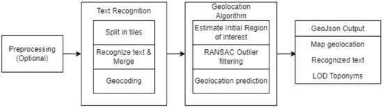
Figure 1.
Overview of the entire pipeline.
The approach does not depend on how the text labels and geocoder matches were generated; therefore, it can be used with any text recognition system and geocoder. The geolocation accuracy largely depends on the text recognition accuracy and geocoder results. If the map is of low quality and most text labels are not recognized, the results will be poor. For each text label, we define its location on the map as the center point of the text detection bounding box. Ideally, we want a list of pixel locations and a correct geocoordinate location for each, allowing the use of all these point pairs to georeference the map. However, since both the text recognition and geocoder results contain errors, we cannot be certain that any toponym and geocoder match is correct. Only the position of each text label on the map is relatively accurate. To get more accurate results, geocoder matches that have a low probability of being correct need to be filtered out. All figures presented in this section refer to the same topographic map of Gent-Melle, from dataset M834 (see Section 4.1). Each figure presents the point pairs currently considered at each step of the algorithm.
3.1. Preprocessing
The dataset of historical topographic map sheets from Belgium contains additional information outside the map boundary. Each map is surrounded by a black border and some blank space, in which coordinate information is given. At each corner, the map is georeferenced based on the 1972 Belgian Datum. The numbers surrounding the map denote the X and Y coordinates in the Belgian Lambert72 projection [20]. This dataset was first preprocessed and the effective map region was determined. It is not strictly necessary to extract the effective map region to geolocate the map. It does make the used techniques slightly more accurate, as the image crop now only contains the map itself, but not the legend, surrounding coordinates, and toponyms. These labels could be incorrectly recognized as toponyms, leading to additional false positives. Figure 2 shows the upper-left corner of one of the topographic maps and the extracted map region.
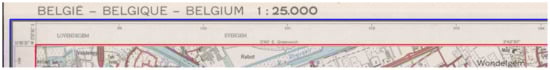
Figure 2.
Outer rectangle detected by morphological operations (in blue), and the effective map region determined via text recognition at the surrounding coordinates (in red).
Morphological operations (erosion and dilation) were used to detect the thick black borders surrounding each map. Next, small crops were taken along the edges of the map. The text within these crops was recognized. For both the left and right side edges, the crops were first rotated so that the X/Y coordinates were upright. We used the location of these surrounding text labels to determine the effective map region. Detection of this inner region with morphological operations alone was inconsistent due to the thin outer edges and slight rotations of some of the scanned maps. After recognizing each text label, the Lambert coordinates were filtered out and the remaining text was used to extract the effective map region. The dataset of contemporary topographic maps did not contain any additional information surrounding the maps and was therefore not preprocessed.
3.2. Text Recognition
Since the images of the map sheets have a much higher resolution than typical images, the performance of the text detection model on the entire dataset was poor. Smaller text labels were consistently not detected when using the full-sized maps. This is likely due to the text detection model using global thresholds to segment the text regions. Therefore, a tiling approach was used to improve results. Previous work showed that larger tile sizes are preferred over smaller ones [10]. Each image was divided into multiple tiles of 2500 × 2500 pixels, with an overlap region (in both X and Y) of 500 pixels. Text detection and recognition was performed on each of the tiles. Text labels detected in the overlap region were merged with overlapping and similar text labels from adjacent tiles to avoid splitting words at the edges of each tile. After merging, the recognized text was post-processed.
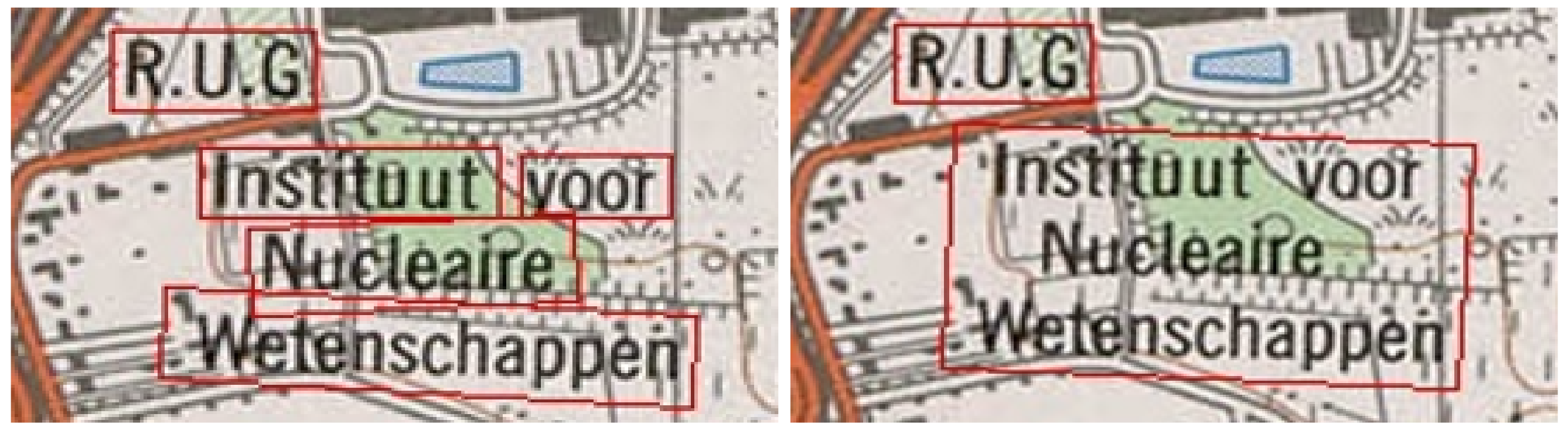
First, the text labels that only contained digits were filtered out. These labels denoted height contours, kilometer milestones, or highway segments and did not provide meaningful results in the following geocoder steps. Next, overlapping detections of multiple text labels were merged, as many toponyms consist of multiple words. This can introduce additional errors by merging incorrectly. Therefore, overlapping detections were only merged if their relative orientations were within 15 degrees of each other. We found that this threshold eliminated most of the incorrectly merged labels. Minor problems still occasionally occurred due to text detection errors and complex arrangements of toponyms. Figure 3 shows one of these complex arrangements, where each detected label overlaps with another and also shows the result after merging.
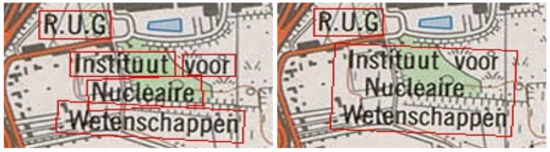
Figure 3.
Example of merging the text labels in the natural reading direction.
When merging multiple overlapping text labels, we sorted them in the natural reading direction. The individual detections were first sorted from top to bottom and divided into different groups based on the difference in their Y-coordinates. Then, each group was sorted individually from left to right, resulting in the natural reading direction. Only text labels (usually denoting rivers) that were read from bottom-left to top-right were sometimes merged incorrectly.
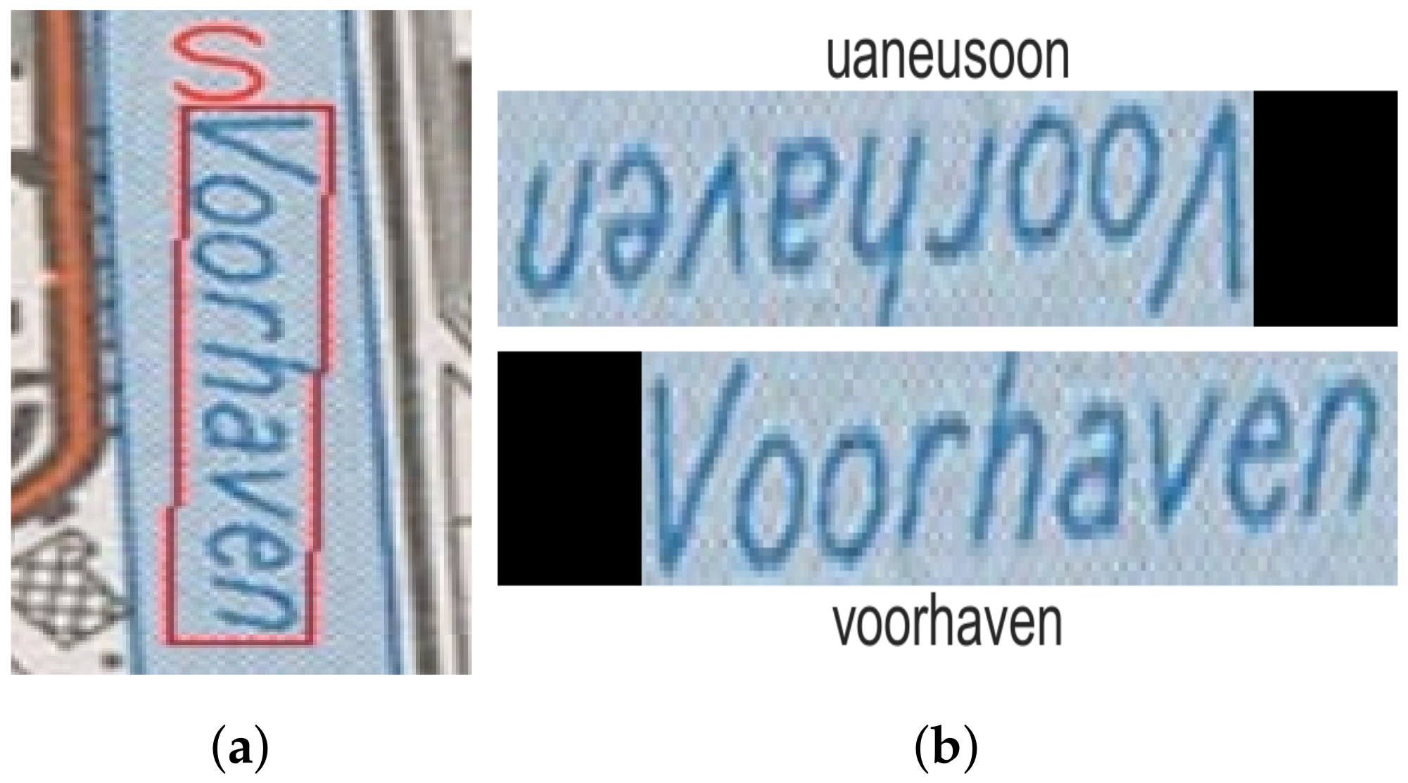
Vertically oriented text was usually detected correctly but often transcribed incorrectly, as can be seen in Figure 4a. As the recognition model assumes that the text is oriented from left to right, such errors occur. After detecting the effective text region, the image crops were warped into horizontally oriented text. If the label was vertically oriented, this transformation needed to be adjusted to warp it correctly. If the leftmost point of a text label is on top, the text is normally read from top-to-bottom. Due to minor errors in text detection, we cannot always rely on the coordinates of the predicted bounding boxes, so two warping transformations are possible. Both image transformations were performed and the text was recognized. In a later step, the incorrect prediction was filtered out using the geocoder results. Figure 4b shows an example of the proposed solution. We suppose a more elegant solution can be used to determine the correct text orientation based on the visual information or the text content. As each map only contains a handful of such vertical text labels, such an improvement was left as future work. As the main goal of this work is to show how off-the-shelf text detection and recognition models can be used to effectively georeference topographic raster maps with little adjustments; no additional processing or linking of the detected text labels was performed.

Figure 4.
An example of the proposed solution for vertically oriented text. (a) The text was incorrectly recognized as the character “s”. (b) Text recognition result after warping the text in both ways.
3.3. Geocoding
After recognizing and processing the text labels on the map, multiple geocoders were queried with each predicted text label. Strings shorter than three characters were ignored as they rarely returned meaningful results. Three different geocoding services were used: Google Geocoding, TomTom Geocoding, and Geonames (open source). We originally intended to only use Geonames but found that many queries did not return meaningful results, while good matches were found with the commercial geocoders. For each geocoder, the resulting toponyms were compared to the query string via the partial string similarity score (https://github.com/seatgeek/thefuzz#partial-ratio accessed on 20 May 2022). Given two strings of length n and m, if the shorter string is length m, the partial string similarity will return the similarity score of the best matching length-m substring. This score is based on the popular Levenshtein distance (https://en.wikipedia.org/wiki/Levenshtein_distance accessed on 20 May 2022). This similarity score ranges from 0 (mismatch) to 100 (perfect substring match). We found that this score performed better than the standard Levenshtein distance, especially for shorter strings. For each match, the toponym name, geocoordinates, similarity, and type (populated place, street, etc.) were saved. As we used multiple geocoders, these results contained duplicates. The duplicates were removed if there was an exact match for the toponym name and type and if both coordinates were close to each other. Checking their closeness is important as two differently located places or streets can have the same name. Some duplicate matches still remained, but these had little effect on the final region of interest.
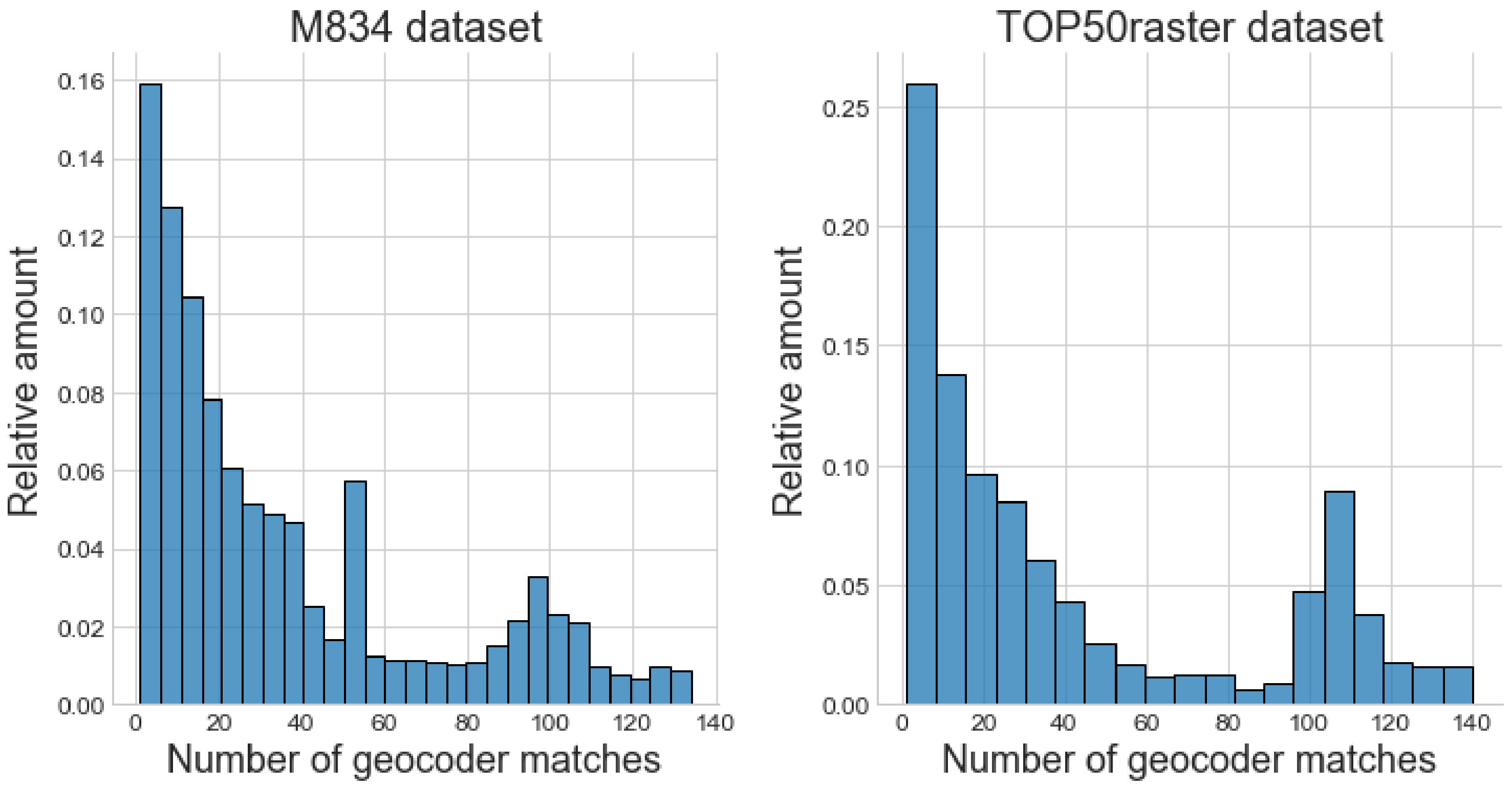
Each map contained an average of 365 and 671 usable text labels for the Belgian (M834) and Dutch (TOP50raster) datasets, respectively. A histogram of the geocoder matches per text label for both datasets is shown in Figure 5. It is clear that the distributions are asymmetric and that most text labels have a small number of matches. The labels with a larger number of matches are the least informative to predict an area of interest, as these denote common place names spread over a large area.

Figure 5.
Histograms show the distribution of the number of geocoder matches per recognized text label for both datasets. Many text labels have a large number of geocoder matches (>50), which do not provide much value.
3.4. Estimating an Initial Region of Interest
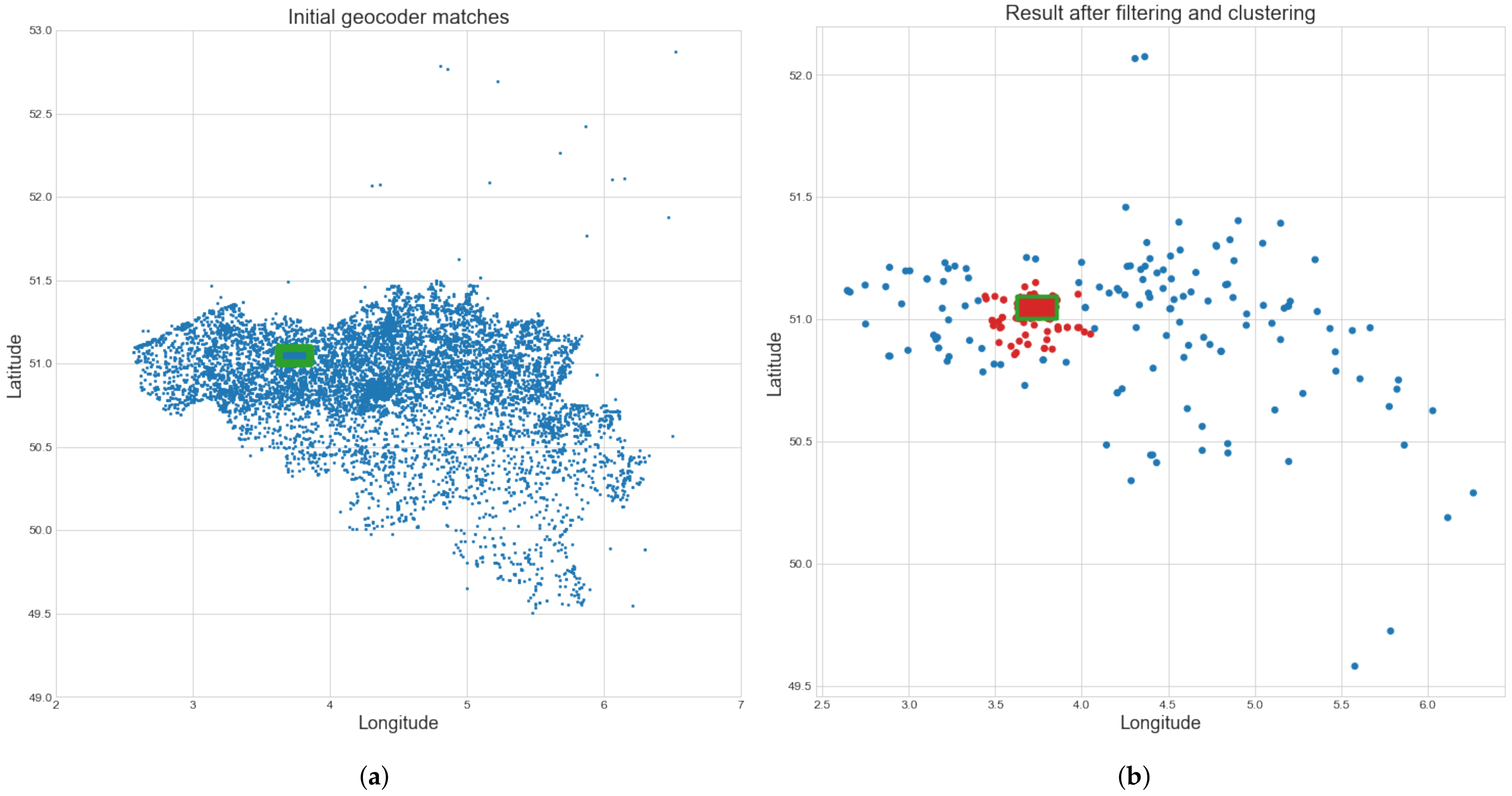
Because some place names are common, certain queries yielded more than 100 geocoder matches. Many street names, such as “Kerkstraat” (comparable to “Main Street” in the USA), are common in Belgian cities. Plotting these coordinates revealed possible matches throughout Belgium and the Netherlands and a small number of random locations around the world. Even though the geocoders allow a country to be specified, the results are not always limited to that country. Most of these geocoder matches were not correct for the queried text. They were either common place and street names or were found due to the fuzzy matching of the geocoders. Figure 6a displays the coordinates of all initial geocoder matches for all recognized text labels on the map of Gent-Melle. Clearly, these are distributed all over Belgium, with some outliers.
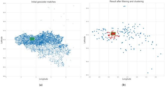
Figure 6.
Coordinates of the initial geocoder matches before and after filtering and clustering. (a) Coordinates of the initial geocoder matches. The green rectangle denotes the ground truth geolocation of the map. The shape of Belgium is visible in the distribution of points (extreme outliers are not shown to improve the visibility of the figure). (b) The result after filtering and clustering of the initial coordinates. The largest cluster found is shown in red. The green rectangle denotes the ground truth geolocation of the map.
Text labels with a large number of matches are therefore not very relevant for predicting an initial region of interest. Similarly, geocoder matches with a lower string similarity with the corresponding text label have a lower probability of being correct. Therefore, we discarded geocoder matches with a partial string similarity below 90. Afterward, text labels that contained more than five geocoder matches were also discarded. In this way, the worst string matches and the most common place names were filtered out. These toponyms were still scattered over hundreds of kilometers and clustering them produced huge regions of interest. Therefore, geocoder matches were also filtered by their relative coordinate distance. Assuming that the correct matches were found, their relative distances should be small and they should be distributed relatively uniformly on the map. Subsequently, each correct coordinate should be relatively close to other correct coordinates. Therefore, the haversine distances between the toponym candidates were calculated and a geocoder match was removed if the distance to any of the five nearest neighbors was greater than 100 km or if the distance to the nearest neighbor was greater than 25 km. This additional filtering ensured that clear outliers were removed. These distance thresholds depend somewhat on the scale of the map. However, most topographic maps contain many toponyms, so the relative distances of correct matches should still be small. For the datasets used, a much smaller distance threshold could be chosen, as each map’s diagonal only covers approximately 19 and 32 km.
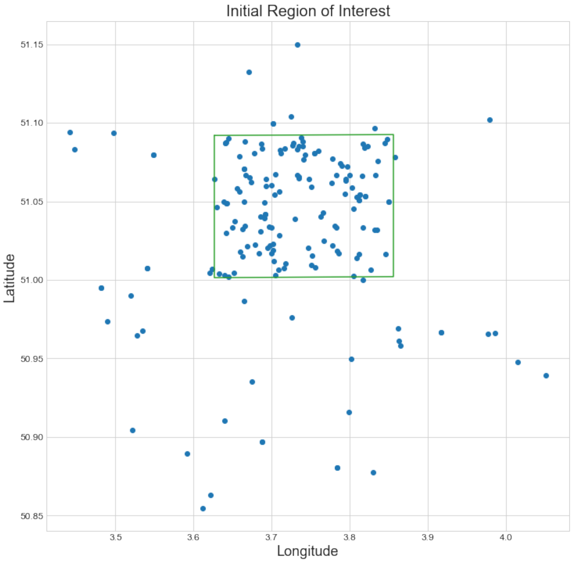
Next, the remaining geocoordinates were clustered with the DBSCAN [21] clustering algorithm, which clusters higher density regions. This clustering eliminated additional outliers and was also used successfully in previous work [15,16]. We used the reciprocal of the number of geocoder matches as a sample weight for each point. In this way, points with multiple matches received a lower weight in clustering. The bounding box of the found cluster was taken as the initial region of interest. If multiple clusters were found, the one containing the most points was selected. Figure 6b displays the result after discarding the low-probability coordinates and clustering. A more detailed plot of the remaining coordinates after determining an initial region of interest for the map of Gent-Melle is shown in Figure 7.
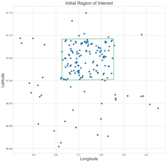
Figure 7.
Coordinates of the geocoder matches that were located inside the initial region of interest. The ground truth geolocation of the map is shown in green.
3.5. Refining the Region of Interest
To refine the initial region of interest, we used both the locations of the text labels and the coordinate locations of their geocoder matches. Generally, the relative pixel location on the map should be very similar to the relative coordinate location of the corresponding toponym match. Similarly, text labels that are further away from each other on the map should have corresponding geocoordinates that are also further away from each other. Naturally, the exact location of the text label will not fully correspond with the correct geocoder coordinates. However, outliers can be filtered out, as this error is quite large on average for incorrect geocoder matches.
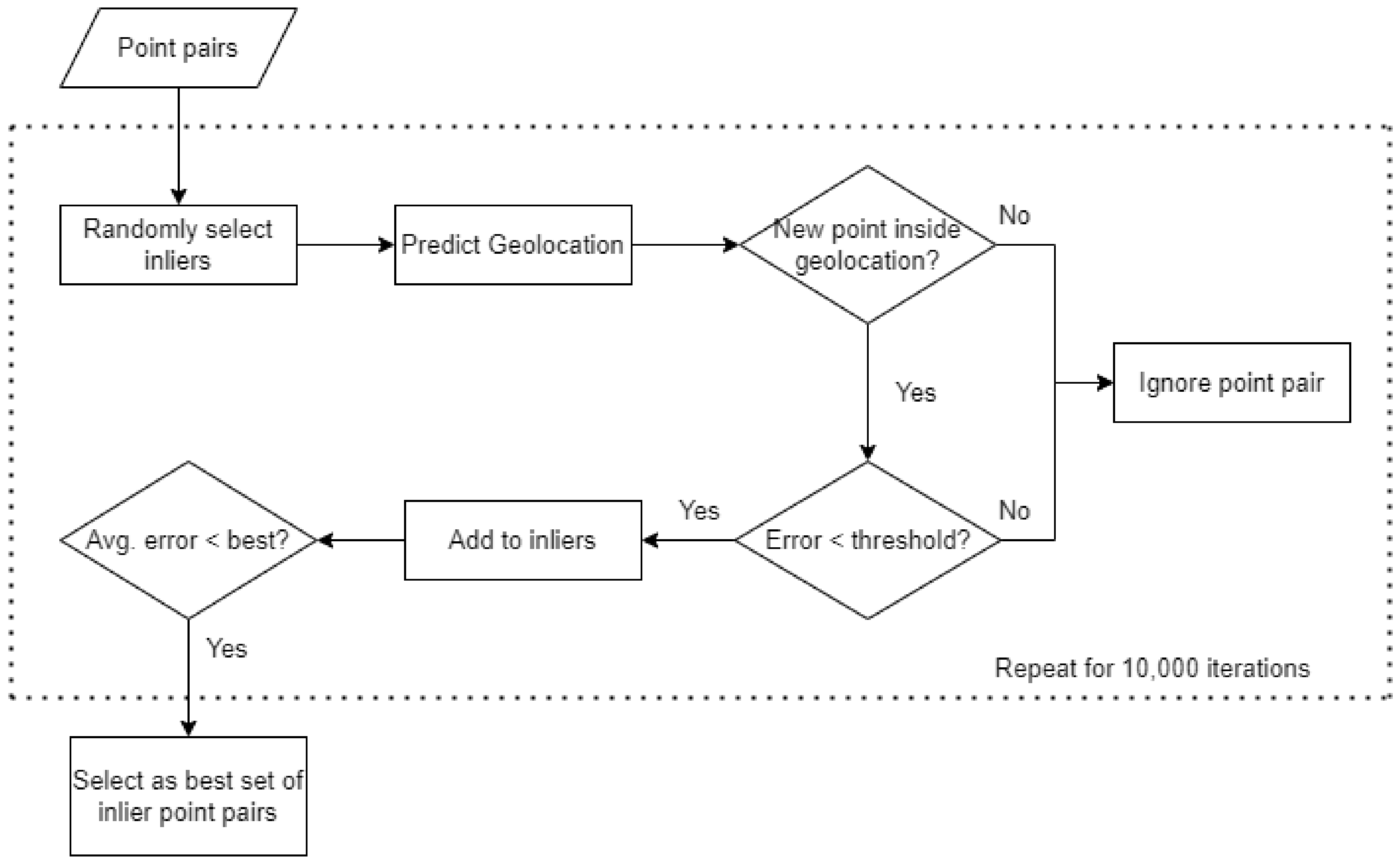
We used a RANSAC-based approach to remove most false-positive coordinate matches. RANSAC is a generic iterative algorithm that can fit a model while still being robust to outliers [22]. Figure 8 gives an overview of the RANSAC-based outlier filtering. First, a set of inlier point pairs was randomly selected from all possible point pairs. Each recognized text label and corresponding pixel location on the raster map was given a 50% probability of being selected. For each selected pixel location, we then randomly chose one of the corresponding geocoordinate matches. This produced a randomized set of point pair inliers. Assuming these inliers were correct, the map geolocation was predicted (see Section 3.6). This geolocation was then used to filter the selection of additional point pairs in the RANSAC algorithm. For each other point pair not initially selected, we performed two checks to decide if these should be added to the set of inliers. First, we checked if the geocoordinates were inside the predicted geolocation. Next, the relative position error (see Section 3.7) was calculated. If the point was inside the geolocation and the error was smaller than a predetermined threshold, we added the point as a candidate inlier. Finally, both the initial inliers and new candidates were used to make a new prediction of the map geolocation and calculate the average relative distance error over all selected point pairs. This entire process was repeated for 10,000 iterations and the set of point pairs with the lowest average error was chosen for further processing.
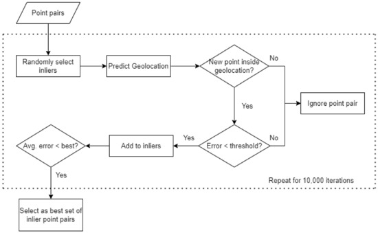
Figure 8.
Overview of the RANSAC outlier filtering algorithm.
3.6. Predicting the Geolocation
As mentioned before, the location of a text label on the raster map does not fully correspond with its corresponding toponym geolocation. There is a slight error for each coordinate pair, as the text label placement depends largely on other geographical features or symbols in that location. If the text label overlaps with the other map features, it is typically moved to provide a better view of the landscape. An underlying feature (river, road, etc.) will not be altered so that a toponym label can be placed more correctly. Combined with the fact that we still cannot guarantee which point pairs are correct, we use the average coordinate vector of all selected point pairs to geolocate the map, to reduce the error in label placement. Even if the toponym labels have a consistent bias contrary to our assumptions, for instance, by making the geolocation corresponds to the top-left corner of the toponym label instead of its center, this would only result in a minor translation error in our final prediction of the control points.
After randomly selecting an initial set of coordinate pair inliers, we estimate the map geolocation assuming that these pairs are correct. This geolocation is then used to filter the selection of additional coordinate pairs in the RANSAC algorithm. First, the average pixel and geocoordinate vectors were calculated, resulting in a central point pair. Next, the absolute vector differences with each point pair and the centers were calculated. The differences in X and Y were calculated independently, as were the differences in longitude and latitude. Afterward, a linear conversion factor between pixel coordinates and geocoordinates was calculated. All of the differences in X were divided by the differences in longitude, and similarly, all the differences in Y were divided by the differences in latitude for each point pair. We now have calculated a conversion factor from pixels to geocoordinates for each point pair and the center points. As the text label position is not perfectly aligned with the corresponding geocoder coordinates, the median for each of these factors was selected, resulting in an average conversion factor from pixel coordinates to geocoordinates. The median is preferred over the mean as it is more robust to outliers. To calculate the conversion factor, we only need two correct point pairs. By taking the median factor of all point pairs, the variance and geolocation error is reduced since it does not fully rely on the correctness of a single pair (which we cannot know). Because the pixel coordinate origin corresponds with the upper left corner of the raster map, the conversion factor for Y must still be multiplied by −1.
After calculating the central coordinate vectors and the conversion factor, the four map corners can be transformed from pixel coordinates to corresponding geocoordinates. Assuming that the predicted geolocation is a rectangle, only the upper left and lower right points need to be transformed to georeference the map. The calculation of the control points is described as a vector equation in Equation (1). Were, and denote the upper left and lower right control points, respectively, and the average geo- and pixel coordinate vectors, denotes the conversion factor, and is a 1D vector containing the width and height of the raster map.
Basically, the translation vector of the average pixel coordinate and map boundaries ([0, 0] and [w, h]) is calculated and multiplied by the conversion factor to get the corresponding translation vector in geocoordinates. This vector is then subtracted from the average geocoordinate to attain the predicted map boundaries in WGS84 coordinates.
3.7. Relative Position Error
In each RANSAC iteration, a set of inlier coordinate pairs was randomly selected and the map region was predicted. For the pair that was not selected, we checked if the geocoordinates were within the predicted map region. If they were, the relative position error was calculated. If this error was smaller than a predetermined threshold, the coordinate pair was added to the set of new candidate inliers. This simple but effective relative position error was calculated by comparing the relative position of each point pair with the inlier point pairs, for both the pixel and geocoordinate locations. We check how many points are to the left/right of the current point on the map and how many points are to the left/right of the associated geocoordinates. We take the difference between these two values and calculate a similar difference for how many points lie above/below the specified pair. Finally, these differences are added and divided by the number of inlier point pairs. This way, the metric is normalized to the total number of inlier pairs considered. The error metric can be calculated very efficiently and will discard many outliers during the randomized inlier candidate selection. We found good results with a threshold of 0.05. So each candidate inlier pair’s relative position needs to “agree” with at least 95% of the initially selected inlier pairs to be selected. After selecting these new candidates, the error metric is calculated for all of the selected point pairs and averaged. The set of point pairs with the lowest average error after 10,000 iterations was then selected for further processing.
3.8. Determining the Final Region of Interest
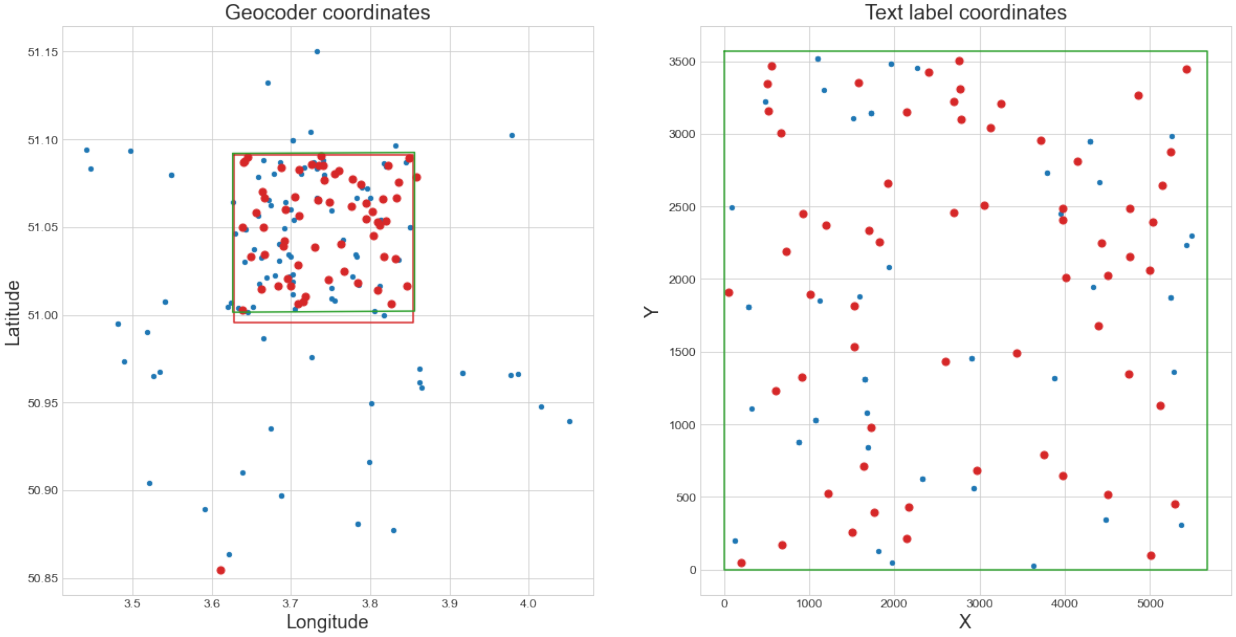
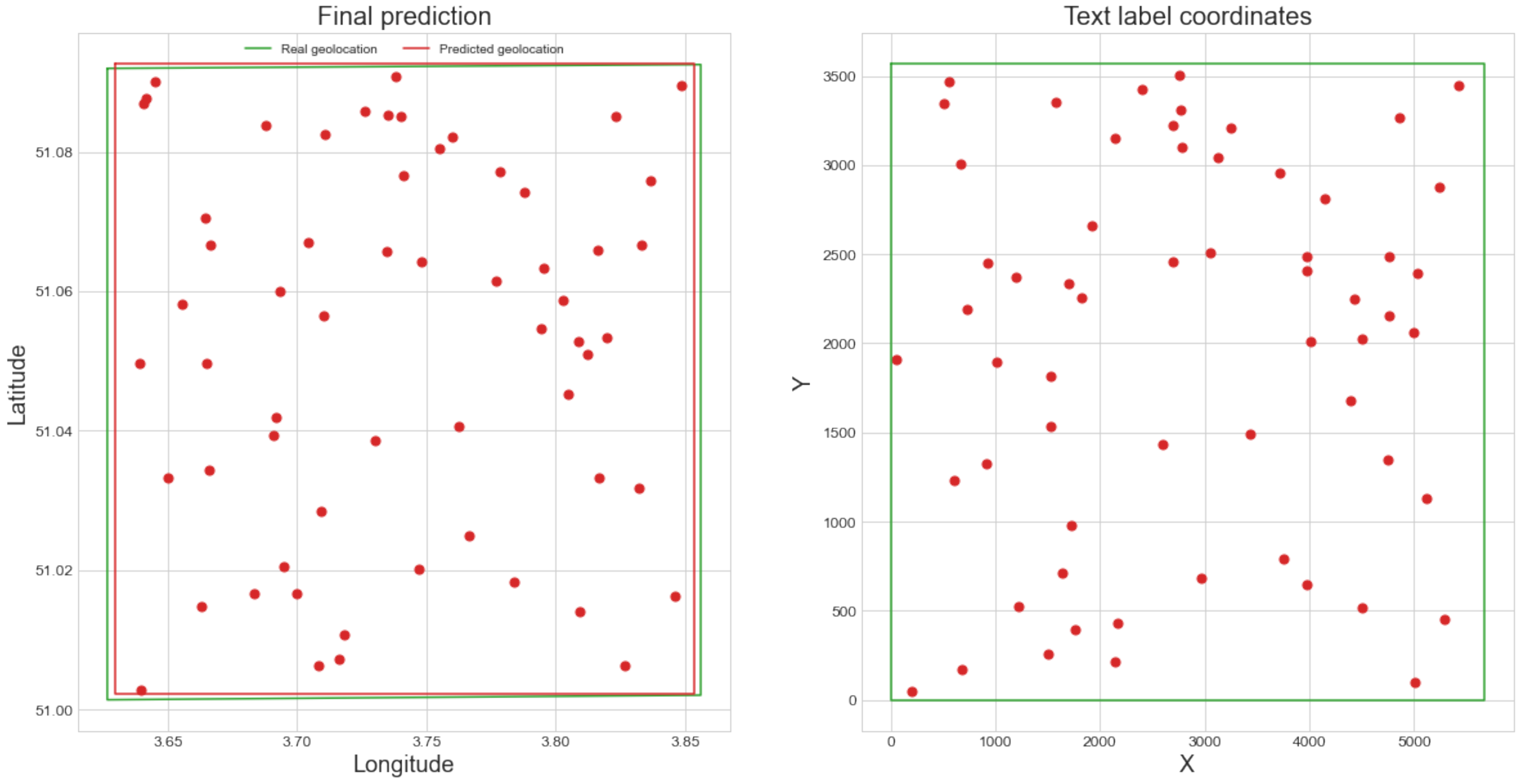
Now that a region of interest has been defined and most of the outlier coordinate pairs have been filtered out with RANSAC, the final geolocation can be estimated. First, the selected coordinate pairs from the previous step were used to predict the map geolocation. This result is shown in Figure 9. After geolocating the map, some geocoder matches can still lie outside the predicted region, either because they are incorrect matches or because the predicted region is incorrect. We iteratively deal with such remaining outliers. We find the outlier geocoordinate point that is farthest from the predicted region, remove that point pair, and predict the geolocation of the map again with all the remaining pairs. We repeat this process until there are no more outliers. The resulting prediction is our best estimate for the map’s geolocation. This iterative outlier filtering process further improved the accuracy of our algorithm. Figure 10 shows the final geolocation estimate and remaining coordinate pairs for the map of Gent-Melle.
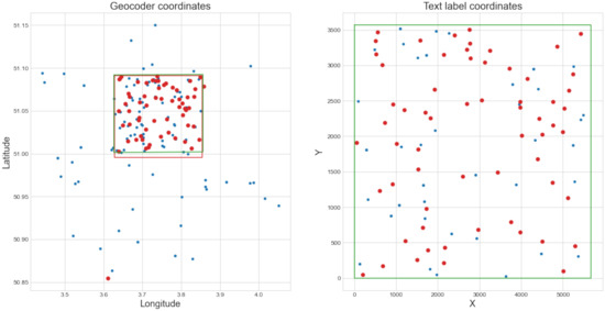
Figure 9.
(Left) Latitude and longitude coordinates of the geocoder matches. The green and red rectangles denote the ground truth geolocation and the predicted geolocation, respectively. Point pairs selected during the RANSAC algorithm are shown in red, the others in blue. (Right) X and Y pixel coordinates of corresponding text labels. The green rectangle denotes the raster map bounds (width and height).
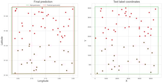
Figure 10.
Final geolocation prediction (in red) and ground truth geolocation (in green) for the map of Gent-Melle. Point pairs used for the prediction are marked in red. There is a visible correlation between the relative positions of the point pairs.
4. Evaluation
This section details the two datasets of topographic raster maps used to validate our techniques. We have chosen a dataset of older maps that were later scanned and digitized, as well as a dataset of contemporary maps generated from topographic vector data. We have applied the same techniques to both datasets and have compared our results in Section 4.2.
4.1. Datasets
- M834 topographic raster maps of Belgium
This dataset consists of 16 adjacent topographic map sheets of Belgium, situated around the city of Ghent. These maps are part of the second edition of the M834 series and they were created between 1980 and 1987 by the Belgian Nationaal Geografisch Instituut (NGI) [23]. The map sheets have a quality of 225 dpi (6300 × 4900 pixels), which is lower than the usually recommended quality of 300 dpi for OCR and text recognition. Each map sheet contains a legend and additional information regarding the projection and geodetic system used. The map sheets were printed at 1:25,000 scale in six colors on offset presses. The average length of the diagonal of each map is approximately 19 km. Each map is surrounded by a black rectangle and some blank space, in which coordinate information is given. At each corner, the map is georeferenced based on the Belgian Datum of 1972. The numbers surrounding the map note the X and Y coordinates in the Belgian Lambert72 projection [20]. To validate the georeferencing of these maps, the ground truth WGS84 coordinates of the bounding polygon for each map were taken from the official metadata provided by the NGI. These maps are subject to copyright, so we are unfortunately unable to share the full raster images. However, the maps can be viewed online in Cartesius (https://www.cartesius.be/CartesiusPortal/ accessed on 20 May 2022). A list of all the selected maps is included with our code. As our georeferencing technique uses the position of the text labels on the map, this dataset was first preprocessed and the effective map region was determined.
- TOP50raster
This dataset consists of 9 adjacent contemporary topographic raster map sheets from the full Top50Raster dataset covering the Netherlands. These 9 maps were created in 2018 and are published on PDOK (https://www.pdok.nl/downloads/-/article/dataset-basisregistratie-topografie-brt-topraster accessed on 20 May 2022), an open-source geospatial data platform, published by the Dutch government. The TOP50raster maps and other raster collections were generalized from the TOP10NL vector data [24]. Each map was generated at a scale of 1:50,000 and the map diagonal measures 32 km on average. Adjacent map sheets were randomly selected from the full collection, links to the original map sheets, and the processed results are included with our code. Each map is stored in the GeoTIFF format [25] and is already georeferenced. The coordinates of the map corners were extracted and converted to WGS84. The images have a quality of 508 dpi (8000 × 10,000 pixels), which is substantially better than the other dataset. There is no additional information surrounding each raster map, so no preprocessing was required.
4.2. Results
The developed techniques were applied to both georeferenced datasets and the resulting predictions were compared to the ground truth geolocations. To evaluate the geolocation predictions, the mean and center georeferencing error distances were calculated. We define the mean distance as the mean haversine distance between all control points (vertices of the ground truth polygon) and the corresponding predictions. We define the center distance as the haversine distance between the predicted map center and the ground truth geolocation center. For each step of the geolocation algorithm, these error distances were calculated. For each dataset, the entire geolocation algorithm was run three times, and the results were averaged and are presented in Table 1.

Table 1.
Geolocalization results for both datasets, with the average map diagonal shown in brackets. The average mean error, maximum mean error, and average center error are presented for each step of the geolocalization algorithm. Prefilter details the result from Section 3.4, without the final clustering step. Initial ROI denotes the result after clustering and refined ROI denotes the result after outlier filtering with RANSAC.
Max. error denotes the largest mean error for any map. Note that the center error distance does not give any indication of how large the predicted map region is compared to the ground truth geolocation and is therefore usually much smaller than the mean error. The average mean error distances for the M834 and TOP50raster datasets were 316 m (1.67% with respect to the map diagonal) and 287 m (0.90%), respectively. The largest mean error distances were 631 m (3.33%) and 438 m (1.37%), respectively. Considering the small error distances with respect to each map’s size, these results are very promising and accurate enough to use in practice. The full results for the M834 dataset are shown in Figure 11. Of the 16 predicted geolocations, 15 have a mean error of less than 500 m and 11 have a center error of less than 200 m.
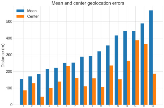
Figure 11.
Mean and center geolocation error distances for each map in the M834 dataset.
5. Discussion
We developed an automatic map processing approach that can extract visible toponyms on raster maps and subsequently georeference these maps with relatively small error. It is surprising that the predictions for the TOP50raster dataset, which contains much larger maps, were better than the other dataset. There are two main reasons for this. First, the maps of TOP50raster are of a higher quality (508 dpi versus 225 dpi), which should lead to better text detection and recognition performance. Second, the average number of detected text labels is nearly twice as high, while the distribution of the number of geocoder matches per text label is similar (see Figure 5). This results in the geolocation algorithm receiving much more valuable information on average, resulting in a better prediction. Detecting more text labels improves the predictions only if they can be matched with the corresponding toponym.
Table 1 shows the improvements for each step in the geolocation algorithm. It is clear that simply clustering the initial geocoder matches gives inaccurate results compared to the final prediction. The error distances also show that the center error is not a good indicator of overall accuracy. As we only compared the predicted and ground truth center; there is no indication of the relative scale of the predicted area. Without filtering, the geolocation algorithm consistently predicted much larger areas than the actual map.
For many applications, an average error of less than 2% is usable. These maps can now be integrated into a GIS with the recognized text labels and matched toponyms as additional metadata. Besides the raster maps themselves, we only used the country information. This was provided to the geocoders to reduce the number of incorrect toponym matches. For most collections, it is trivial to provide the country information to the algorithm. For maps depicting border regions of countries, it can be beneficial to include both countries in the geocoder requests. Besides querying the recognized text labels with the geocoders, the entire processing pipeline, from text detection and recognition to geolocation prediction, is relatively fast. The calculations necessary to perform the outlier filtering and to calculate the error metric presented in Section 3.7 were nearly all vectorized and are therefore very performant.
However, it remains difficult to determine if the georeferencing predictions were accurate automatically. This is a classic problem that plagues many unsupervised approaches, as no labeled data would be available when using this technique in practice. We can, however, perform some extra validations, given that the raster map is part of a uniform series (which is usually the case for topographic maps). For instance, if the height or width of the predicted geolocation for a map is much greater than the other predictions, we can assume that this prediction is less accurate. Additionally, if the order of the map sheets is known, geolocations that failed can also be detected, as these will have much greater overlap with the other predictions. Of course, these validation techniques are not very robust and will only work if a majority of the predictions were relatively correct.
The backbone of this pipeline is the determination of the initial region of interest. Because density-based clustering was used, this determination assumes that the text recognition was usable and that the number of false-positive geocoder matches is relatively small compared to the number of correct matches. Therefore, the two main failure cases of the geolocation approach occur when the map is of low quality, resulting in poor text recognition results, or when the text labels are consistently split into multiple, far away words or presented in complex arrangements. Text recognition techniques that can work with low-quality images, such as [26], could be used to improve results. But usually, this is not an issue when analyzing raster maps. The main issue is often the correct linking of text labels with the same location phrase. This was not the focus of our research and is not a trivial task to solve, as the impressive work in [16] shows. Even with a complex technique to correctly link text labels, some errors remained. In that study, only the center of each map was geolocated. The center of the largest cluster of geocoder matches was taken as a prediction for the map center, which resulted in errors of 27%, 48%, and 51% with the ground truth center, relative to the map diagonals, for the three maps discussed in detail. Without any text linking, these errors were over 91%, clearly demonstrating its importance in predicting an initial region of interest.
Even though we are satisfied with the results presented, we believe that there is still much room for improvement. Mainly the text linking and geocoder querying need improvement, as these are key in predicting a correct initial region of interest. Adding additional semantic information can also help determine more robust geolocations. Currently, each text label and corresponding toponym is naively considered as a point. These toponyms often do not represent single points, but lines and polygons. Clearly, this is not the optimal way to deal with these types of features. Additionally, text labels that denote visible features on the map, such as rivers and streets, could be used in conjunction with the visual content to geolocate these more accurately. It can also be beneficial to give different features a higher weight, depending on their type. For instance, a street name may provide more useful and localized information than a place name. Finally, more work needs to be done on developing an effective strategy to validate the predicted geolocation in an unsupervised way. It can be valuable to know if the predictions were not accurate for certain maps in the dataset; these can then be corrected manually.
6. Conclusions
We have developed an automatic technique to georeference topographic raster maps using pretrained text recognition models and geocoders. Two datasets were processed, resulting in an average error of 316 m (1.67%) and 287 m (0.90%) for maps spanning 19 km and 32 km, respectively. With average errors within 2% of the map size, these maps can now be accurately queried for a specific region of interest. The georeferenced maps can then be integrated into a GIS with the recognized text labels and linked open data toponyms as additional metadata for each raster map in the collection. This additional metadata greatly improves the quality and accessibility of the dataset.
Author Contributions
Conceptualization, Kenzo Millevile, Steven Verstockt, and Nico Van de Weghe; methodology, Kenzo Milleville; software, Kenzo Milleville; validation, Kenzo Milleville; formal analysis, Kenzo Milleville; investigation, Kenzo Milleville; resources, Kenzo Milleville; data curation, Kenzo Milleville; writing—original draft preparation, Kenzo Millevile, Steven Verstockt, and Nico Van de Weghe; writing—review and editing, Kenzo Millevile, Steven Verstockt, and Nico Van de Weghe; visualization, Kenzo Milleville; supervision, Steven Verstockt, and Nico Van de Weghe; project administration, Steven Verstockt and Nico Van de Weghe; funding acquisition, Steven Verstockt and Nico Van de Weghe All authors have read and agreed to the published version of the manuscript.
Funding
This research received no external funding.
Institutional Review Board Statement
Not applicable.
Informed Consent Statement
Not applicable.
Data Availability Statement
The data that supports the findings of this research is openly available at: https://github.com/kymillev/geolocation (accessed on 20 May 2022).
Acknowledgments
We sincerely thank Haosheng Huang for his contributions to the paper and the advice given during the research.
Conflicts of Interest
The authors declare no conflict of interest.
References
- Crăciunescu, V.; Constantinescu, Ş.; Ovejanu, I.; Rus, I. Project eHarta: A collaborative initiative to digitally preserve and freely share old cartographic documents in Romania. e-Perimetron 2011, 6, 261–269. [Google Scholar]
- Fleet, C.; Kowal, K.C.; Pridal, P. Georeferencer: Crowdsourced georeferencing for map library collections. D-Lib Mag. 2012, 18, 52. [Google Scholar] [CrossRef]
- Waters, T. Map Warper. 2020. Available online: https://mapwarper.net/ (accessed on 20 May 2022).
- Pezeshk, A.; Tutwiler, R.L. Automatic feature extraction and text recognition from scanned topographic maps. IEEE Trans. Geosci. Remote Sens. 2011, 49, 5047–5063. [Google Scholar] [CrossRef]
- Bissacco, A.; Cummins, M.; Netzer, Y.; Neven, H. Photoocr: Reading text in uncontrolled conditions. In Proceedings of the IEEE International Conference on Computer Vision, Sydney, NSW, Australia, 1–8 December 2013; pp. 785–792. [Google Scholar]
- Tafti, A.P.; Baghaie, A.; Assefi, M.; Arabnia, H.R.; Yu, Z.; Peissig, P. OCR as a service: An experimental evaluation of Google Docs OCR, Tesseract, ABBYY FineReader, and Transym. In Proceedings of the International Symposium on Visual Computing, Las Vegas, NV, USA, 12–14 December 2016; pp. 735–746. [Google Scholar]
- Karatzas, D.; Gomez-Bigorda, L.; Nicolaou, A.; Ghosh, S.; Bagdanov, A.; Iwamura, M.; Matas, J.; Neumann, L.; Chandrasekhar, V.R.; Lu, S.; et al. ICDAR 2015 competition on robust reading. In Proceedings of the 2015 13th International Conference on Document Analysis and Recognition (ICDAR), Tunis, Tunisia, 23–26 August 2015; pp. 1156–1160. [Google Scholar]
- Veit, A.; Matera, T.; Neumann, L.; Matas, J.; Belongie, S. Coco-text: Dataset and benchmark for text detection and recognition in natural images. arXiv 2016, arXiv:1601.07140. [Google Scholar]
- Baek, J.; Kim, G.; Lee, J.; Park, S.; Han, D.; Yun, S.; Oh, S.J.; Lee, H. What is wrong with scene text recognition model comparisons? dataset and model analysis. In Proceedings of the IEEE International Conference on Computer Vision, Seoul, Korea, 27 October–2 November 2019; pp. 4715–4723. [Google Scholar]
- Milleville, K.; Verstockt, S.; Van de Weghe, N. Improving toponym recognition accuracy of historical topographic maps. In International Workshop on Automatic Vectorisation of Historical Maps; Department of Cartography and Geoinformatics, ELTE Eötvös Loránd University: Budapest, Hungary, 2020. [Google Scholar]
- Abkenar, S.; Ahmadyfard, A. Text Extraction from Raster Maps Using Color Space Quantization. CS IT Conf. Proc. 2017, 7, 77–86. [Google Scholar] [CrossRef]
- Höhn, W. Detecting arbitrarily oriented text labels in early maps. In Proceedings of the Iberian Conference on Pattern Recognition and Image Analysis, Madeira, Portugal, 5–7 June 2013; pp. 424–432. [Google Scholar]
- Chiang, Y.Y.; Knoblock, C.A. Recognizing text in raster maps. Geoinformatica 2015, 19, 1–27. [Google Scholar] [CrossRef]
- Weinman, J. Geographic and style models for historical map alignment and toponym recognition. In Proceedings of the 2017 14th IAPR International Conference on Document Analysis and Recognition (ICDAR), Kyoto, Japan, 9–15 November 2017; Volume 1, pp. 957–964. [Google Scholar]
- Tavakkol, S.; Chiang, Y.Y.; Waters, T.; Han, F.; Prasad, K.; Kiveris, R. Kartta labs: Unrendering historical maps. In Proceedings of the 3nd ACM SIGSPATIAL International Workshop on AI for Geographic Knowledge Discovery, Seattle, WA, USA, 5 November 2019; pp. 48–51. [Google Scholar]
- Li, Z.; Chiang, Y.Y.; Tavakkol, S.; Shbita, B.; Uhl, J.H.; Leyk, S.; Knoblock, C.A. An Automatic Approach for Generating Rich, Linked Geo-Metadata from Historical Map Images. In Proceedings of the 26th ACM SIGKDD International Conference on Knowledge Discovery & Data Mining, Virtual Event, 23–27 August 2020; pp. 3290–3298. [Google Scholar]
- Baek, Y.; Lee, B.; Han, D.; Yun, S.; Lee, H. Character region awareness for text detection. In Proceedings of the IEEE Conference on Computer Vision and Pattern Recognition, Long Beach, CA, USA, 16–17 June 2019; pp. 9365–9374. [Google Scholar]
- Shi, B.; Bai, X.; Yao, C. An End-to-End Trainable Neural Network for Image-Based Sequence Recognition and Its Application to Scene Text Recognition. IEEE Trans. Pattern Anal. Mach. Intell. 2017, 39, 2298–2304. [Google Scholar] [CrossRef] [PubMed] [Green Version]
- Zhou, X.; Yao, C.; Wen, H.; Wang, Y.; Zhou, S.; He, W.; Liang, J. East: An efficient and accurate scene text detector. In Proceedings of the IEEE Conference on Computer Vision and Pattern Recognition, Honolulu, HI, USA, 21–26 July 2017; pp. 5551–5560. [Google Scholar]
- Donnay, J.P.; Lambot, P. Geodetic and cartographical standards applied in Belgium. Concise Geogr. Belg. 2012, 1, 41–42. [Google Scholar]
- Ester, M.; Kriegel, H.P.; Sander, J.; Xu, X. A Density-Based Algorithm for Discovering Clusters in Large Spatial Databases with Noise. In Proceedings of the Second International Conference on Knowledge Discovery and Data Mining (KDD’96), Portland, OR, USA, 2–4 August 1996; pp. 226–231. [Google Scholar]
- Fischler, M.A.; Bolles, R.C. Random sample consensus: A paradigm for model fitting with applications to image analysis and automated cartography. Commun. ACM 1981, 24, 381–395. [Google Scholar] [CrossRef]
- De Maeyer, P.; De Vliegher, B.M.; Brondeel, M. Spiegel van de Wereld; Academia Press: Gent, Belgium, 2004. [Google Scholar]
- Stoter, J.E.; Kraak, M.J.; Knippers, R. Generalization of framework data: A research agenda. In Proceedings of the ICA Workshop on “Generalisation and Multiple Representation”, Leicester, UK, 20–21 August 2004; pp. 20–21. [Google Scholar]
- Ritter, N.; Ruth, M. The GeoTiff data interchange standard for raster geographic images. Int. J. Remote Sens. 1997, 18, 1637–1647. [Google Scholar] [CrossRef]
- Wang, W.; Xie, E.; Sun, P.; Wang, W.; Tian, L.; Shen, C.; Luo, P. TextSR: Content-aware text super-resolution guided by recognition. arXiv 2019, arXiv:1909.07113. [Google Scholar]


Publisher’s Note: MDPI stays neutral with regard to jurisdictional claims in published maps and institutional affiliations. |
© 2022 by the authors. Licensee MDPI, Basel, Switzerland. This article is an open access article distributed under the terms and conditions of the Creative Commons Attribution (CC BY) license (https://creativecommons.org/licenses/by/4.0/).