
Susceptibility Mapping of Typical Geological Hazards in Helong City Affected by Volcanic Activity of Changbai Mountain, Northeastern China

Abstract
:1. Introduction
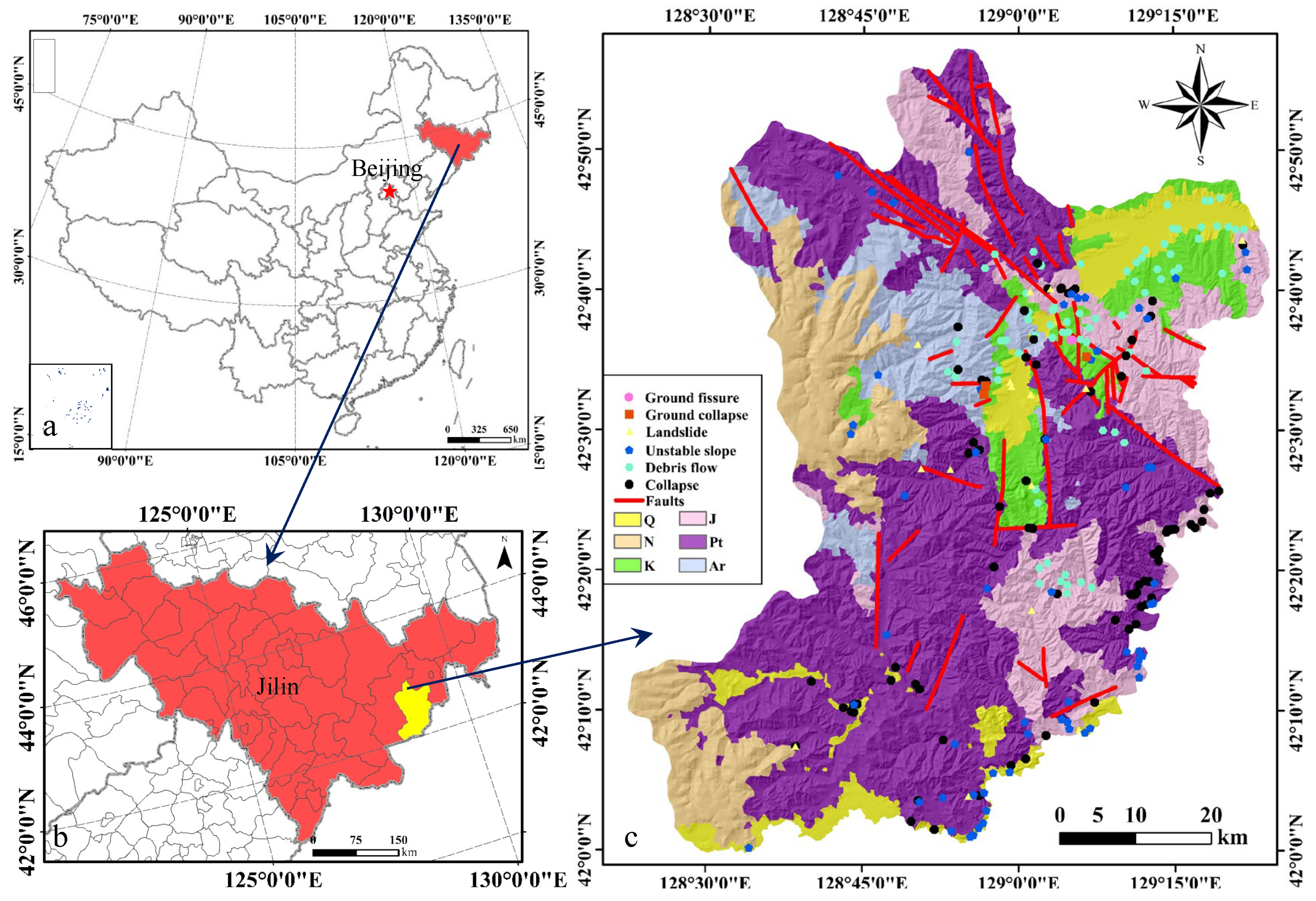
2. Study Area
3. Methods and Data
3.1. Geological Hazard Inventory Data
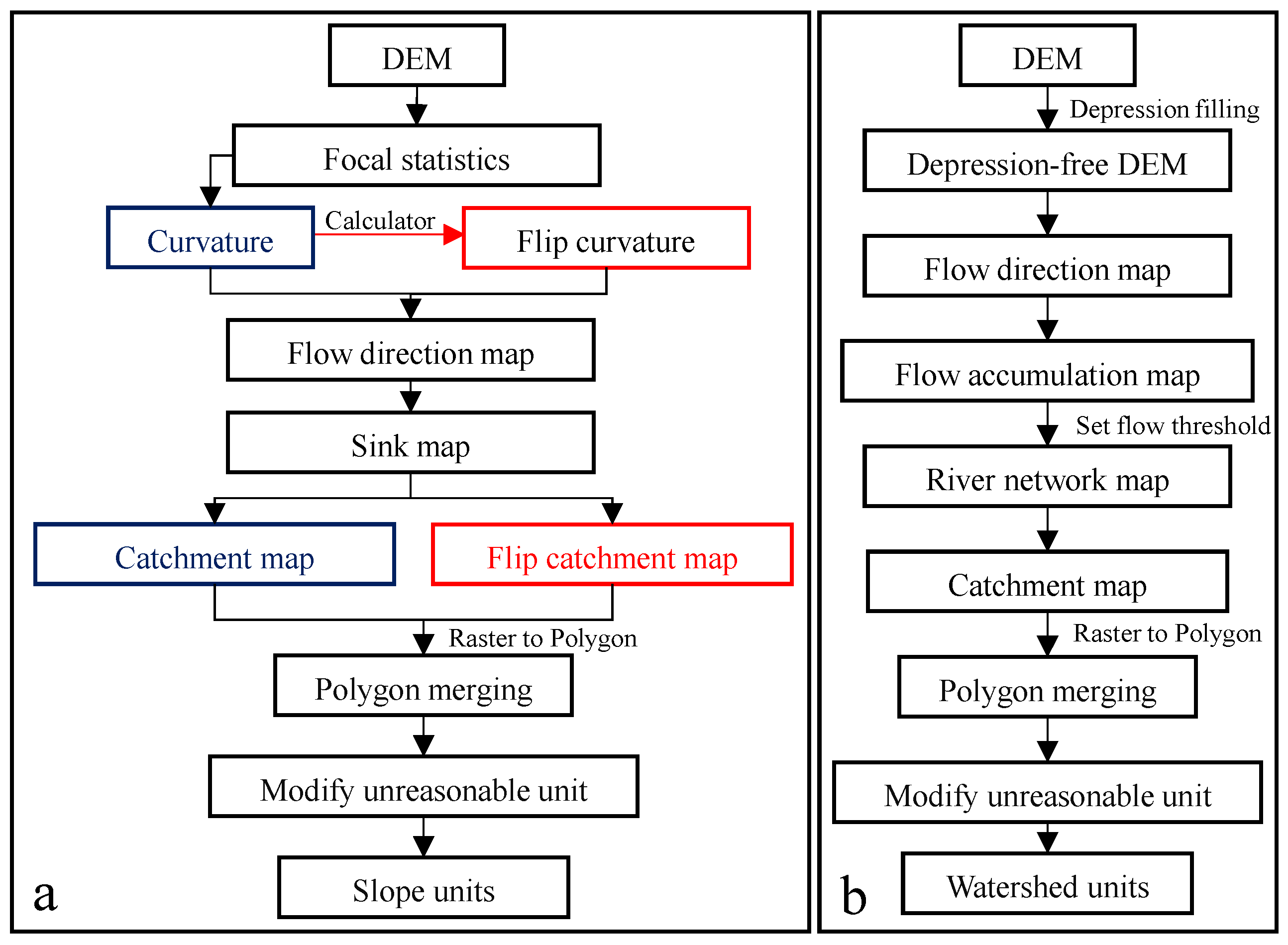
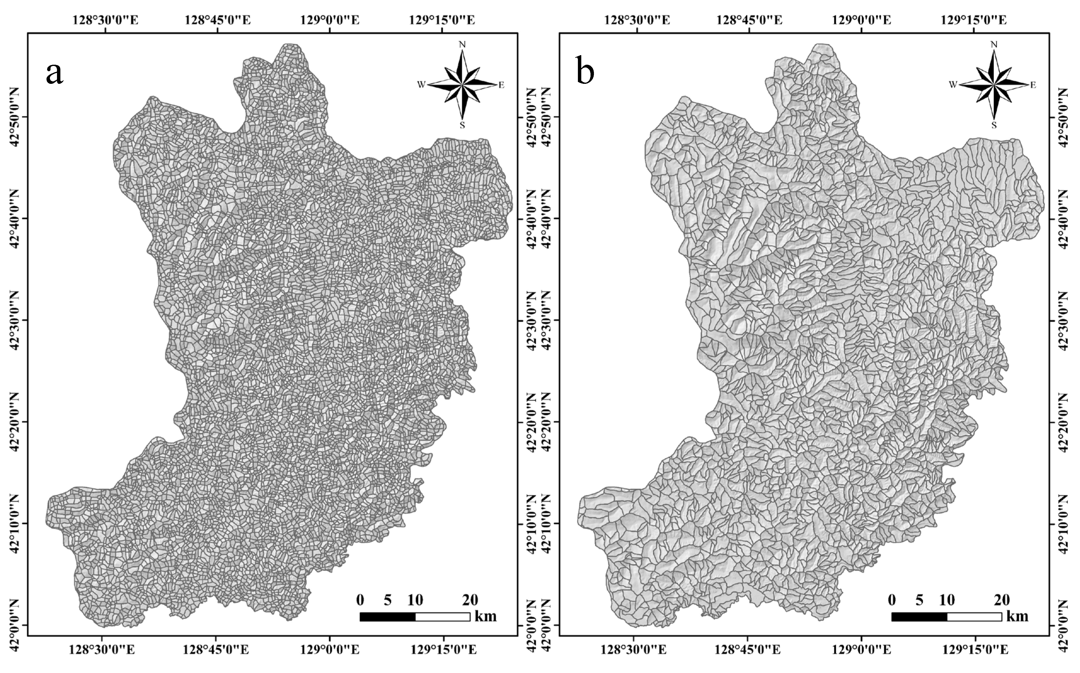
3.2. Mapping Unit
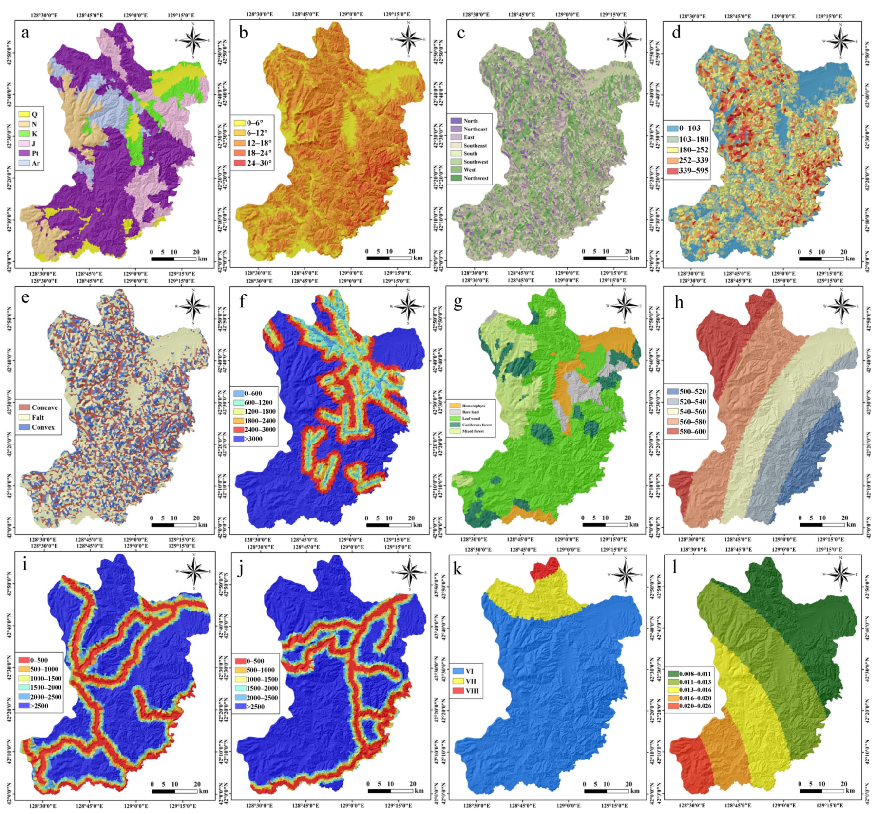
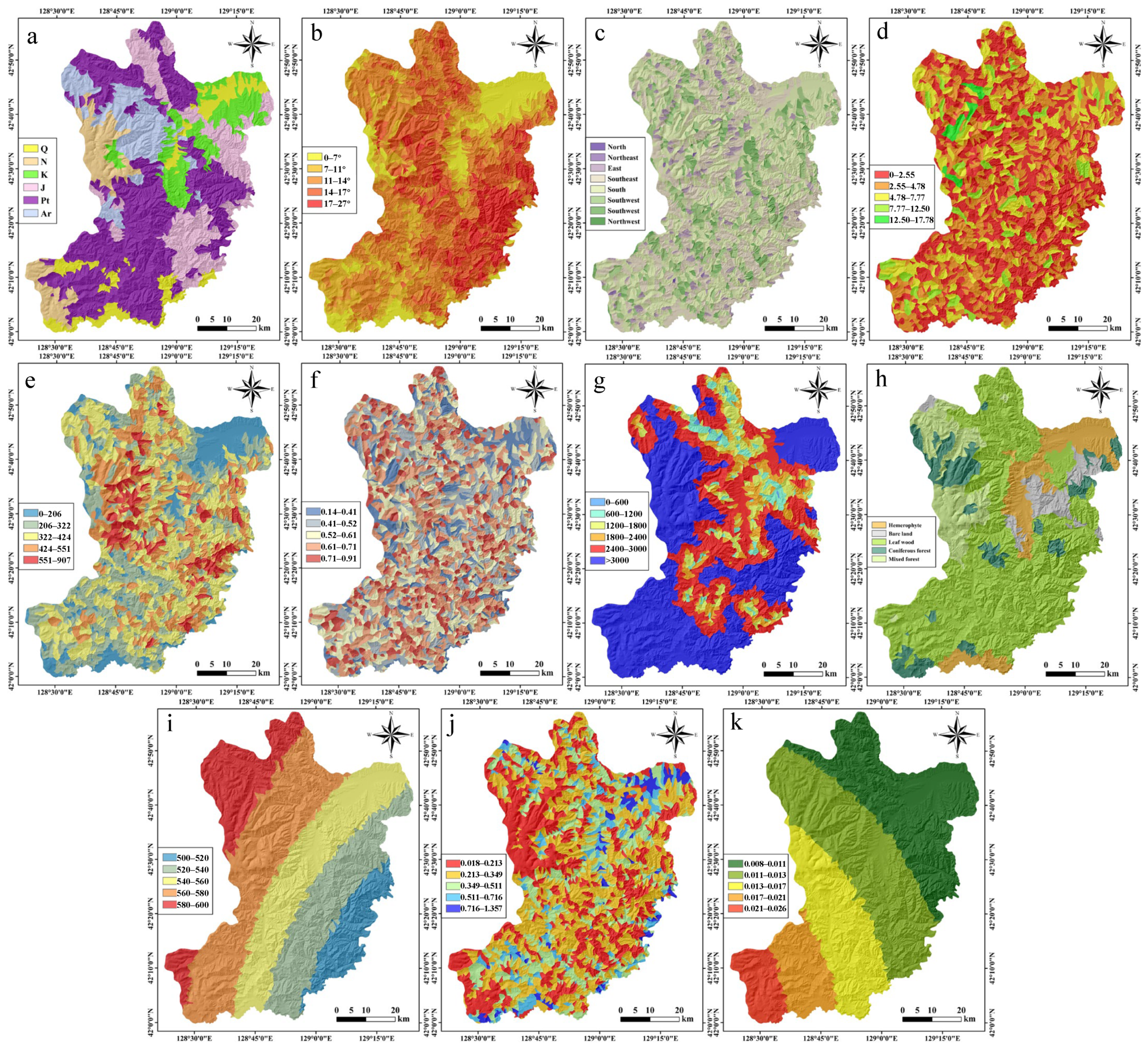
3.3. Conditioning Factors
3.3.1. Establishment of the Conditioning Factors System
3.3.2. Multicollinearity Analysis
3.4. Geological Disaster-Susceptibility Model
3.4.1. Support Vector Machine
3.4.2. Artificial Neural Network
3.5. Validation Methods
3.5.1. Receiver Operating Characteristic Curve
3.5.2. Statistical Parameters
3.5.3. Cross Validation
3.6. The Importance of Conditioning Factors
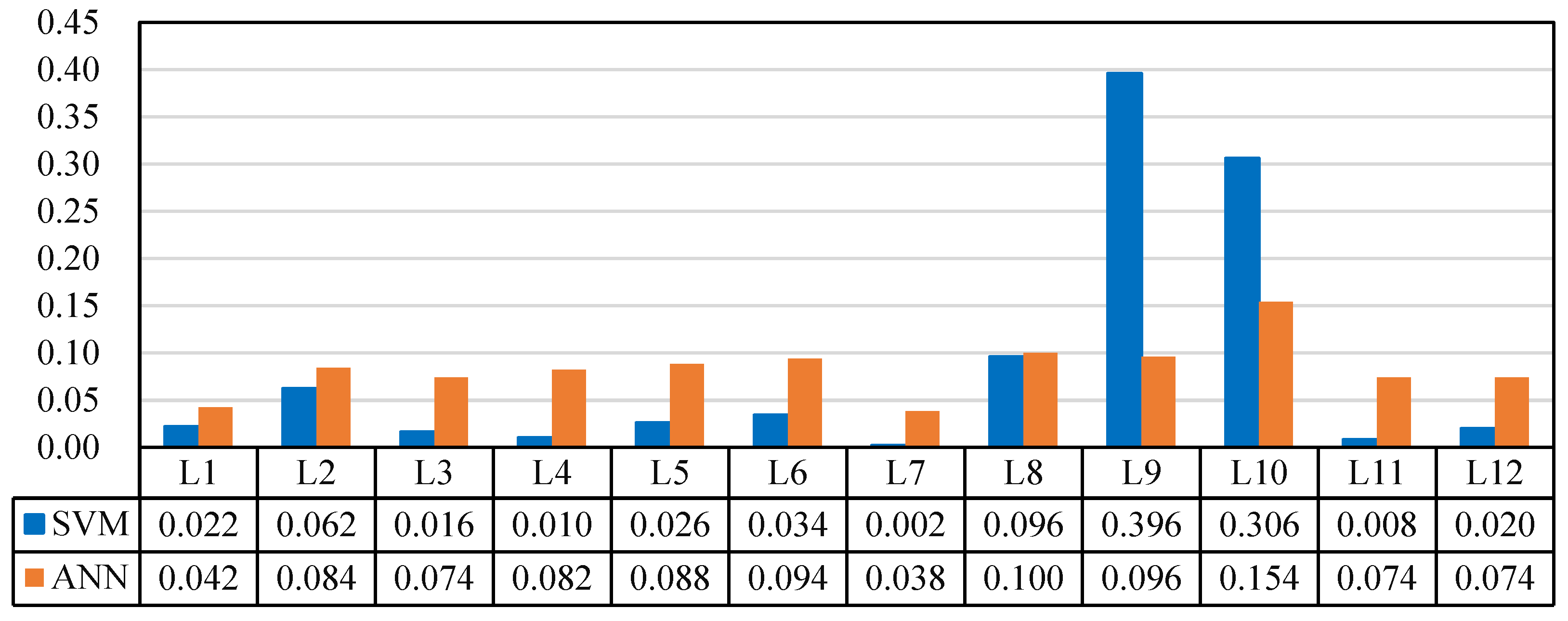
3.6.1. Variance-Based Method
3.6.2. Frequency Ratio Method
4. Results and Discussion
4.1. Multicollinearity Analysis Results
4.2. Modeling Results and Comparison
4.2.1. Modeling Results
4.2.2. Landslide-Susceptibility Model Comparison
4.2.3. Debris Flow Susceptibility Model Comparison
4.2.4. Comparison with Other Models
4.3. Analysis of Importance of Conditioning Factors
4.3.1. Analysis of Importance of Landslide Conditioning Factors
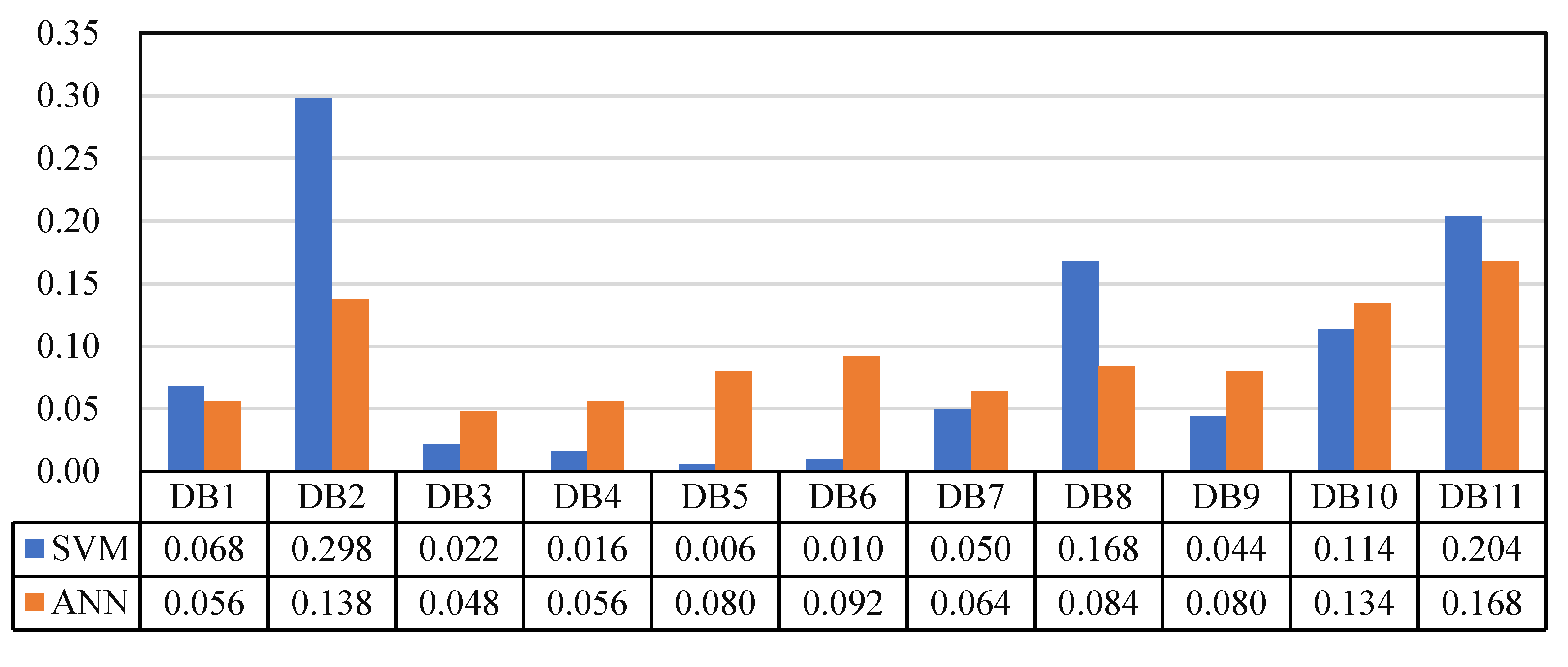
4.3.2. Analysis of Importance of Debris Flow Conditioning Factors
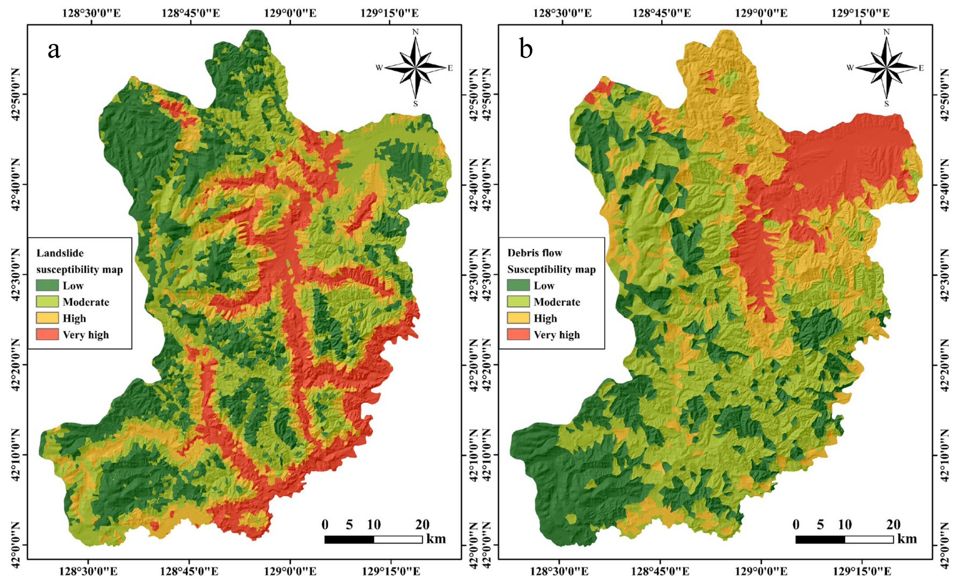
4.4. Geological Hazard-Susceptibility Map Analysis
5. Conclusions
- (1)
- According to the modeling results, the SVM model is better than the ANN model for both the landslide susceptibility mapping and debris flow susceptibility mapping. The landslide susceptibility map modeled by the SVM model shows that the areas with low, moderate, high, and very high landslide susceptibility are 31.58%, 33.15%, 17.07%, and 18.19% of the total study area, respectively. Moreover, the high and very high landslide susceptibility classes make up 85.54% of the known landslides. The areas with low, moderate, high, and very high debris flow susceptibility are 25.63%, 38.19%, 23.47%, and 12.71% of the total study area, respectively, with high and very high debris flow susceptibility classes accounting for 80.55% of the known debris flows.
- (2)
- Distance to river, distance to road, and average annual rainfall were the three most significant factors for landslide susceptibility mapping; and slope angle, volcanic earthquake, land use, and geomorphic information entropy were the four most significant factors for debris flow susceptibility mapping.
- (3)
- From the landslide susceptibility and debris flows susceptibility map results, it can be seen that the very high and high landslide and debris flow susceptibility are mainly distributed in areas of lower elevation, and mainly distributed around the cities and towns in Helong City. Thus, it is suggested to strengthen disaster monitoring in these areas, realize real-time monitoring and early warning of geological disasters, and pay attention to the deployment of disaster prevention and mitigation.
Author Contributions
Funding
Data Availability Statement
Acknowledgments
Conflicts of Interest
References
- Liu, X. Hazard Assessment of Landslide and Collapse Induced by Volcanic Eruption in Changbai Mountains. Master’s Thesis, Jilin University, Changchun, China, 2016. [Google Scholar]
- Liu, G.S.H.; Guo, F. The newest monitoring information of Changbaishan volcano, NE China. Acta Petrol. Sin. 2011, 27, 2905–2911. [Google Scholar]
- Blais-Stevens, A.; Behnia, P.; Kremer, M.; Page, A.; Kung, R.; Bonham-Carter, G. Landslide susceptibility mapping of the Sea to Sky transportation corridor, British Columbia, Canada: Comparison of two methods. Bull. Eng. Geol. Environ. 2012, 71, 447–466. [Google Scholar] [CrossRef]
- Kayastha, P.; Dhital, M.R.; De Smedt, F. Evaluation and comparison of GIS based landslide susceptibility mapping procedures in Kulekhani watershed, Nepal. J. Geol. Soc. India 2013, 81, 219–231. [Google Scholar] [CrossRef]
- Van Westen, C.J.; Rengers, N.; Soeters, R. Use of geomorphological information in indirect landslide susceptibility assessment. Nat. Hazards 2003, 30, 399–419. [Google Scholar] [CrossRef]
- Steger, S.; Bell, R.; Petschko, H.; Glade, T. Evaluating the Effect of Modelling Methods and Landslide Inventories Used for Statistical Susceptibility Modelling. In Proceedings of the 12th International IAEG Congress, Torino, Italy, 15–19 September 2015; pp. 201–204. [Google Scholar]
- Sun, X.; Chen, J.; Bao, Y.; Han, X.; Zhan, J.; Peng, W. Landslide Susceptibility Mapping Using Logistic Regression Analysis along the Jinsha River and Its Tributaries Close to Derong and Deqin County, Southwestern China. Isprs Int. J. Geo-Inf. 2018, 7, 438. [Google Scholar] [CrossRef] [Green Version]
- Sun, X.; Chen, J.; Han, X.; Bao, Y.; Zhan, J.; Peng, W. Application of a GIS-based slope unit method for landslide susceptibility mapping along the rapidly uplifting section of the upper Jinsha River, South-Western China. Bull. Eng. Geol. Environ. 2020, 79, 533–549. [Google Scholar] [CrossRef]
- Sun, X.; Chen, J.; Han, X.; Bao, Y.; Zhou, X.; Peng, W. Landslide susceptibility mapping along the upper Jinsha River, south-western China: A comparison of hydrological and curvature watershed methods for slope unit classification. Bull. Eng. Geol. Environ. 2020, 79, 4657–4670. [Google Scholar] [CrossRef]
- Leventhal, A.R.; Kotze, G.P. Landslide susceptibility and hazard mapping in Australia for land-use planning—With reference to challenges in metropolitan suburbia. Eng. Geol. 2008, 102, 238–250. [Google Scholar] [CrossRef]
- Segoni, S.; Tofani, V.; Rosi, A.; Catani, F.; Casagli, N. Combination of Rainfall Thresholds and Susceptibility Maps for Dynamic Landslide Hazard Assessment at Regional Scale. Front. Earth Sci. 2018, 6, 85. [Google Scholar] [CrossRef] [Green Version]
- Shit, P.K.; Bhunia, G.S.; Maiti, R. Potential landslide susceptibility mapping using weighted overlay model (WOM). Modeling Earth Syst. Environ. 2016, 2, 21. [Google Scholar] [CrossRef] [Green Version]
- Farahani, S.; Behnam, B.; Tahershamsi, A. Macrozonation of seismic transient and permanent ground deformation of Iran. Nat. Hazards Earth Syst. Sci. 2020, 20, 2889–2903. [Google Scholar] [CrossRef]
- Farahani, S.; Tahershamsi, A.; Behnam, B. Earthquake and post-earthquake vulnerability assessment of urban gas pipelines network. Nat. Hazards 2020, 101, 327–347. [Google Scholar] [CrossRef]
- Binita, K.C.; Shepherd, J.M.; King, A.W.; Johnson Gaither, C. Multi-hazard climate risk projections for the United States. Nat. Hazards 2021, 105, 1963–1976. [Google Scholar] [CrossRef]
- Guzzetti, F.; Mondini, A.C.; Cardinali, M.; Fiorucci, F.; Santangelo, M.; Chang, K.-T. Landslide inventory maps: New tools for an old problem. Earth-Sci. Rev. 2012, 112, 42–66. [Google Scholar] [CrossRef] [Green Version]
- Dai, K.; Li, Z.; Tomas, R.; Liu, G.; Yu, B.; Wang, X.; Cheng, H.; Chen, J.; Stockamp, J. Monitoring activity at the Daguangbao mega-landslide (China) using Sentinel-1 TOPS time series interferometry. Remote Sens. Environ. 2016, 186, 501–513. [Google Scholar] [CrossRef] [Green Version]
- Zhao, C.; Kang, Y.; Zhang, Q.; Zhu, W.; Li, B.; IEEE. Landslide detection and monitoring with insar technique over upper reaches of jinsha river, China. In Proceedings of the 36th IEEE International Geoscience and Remote Sensing Symposium (IGARSS), Beijing, China, 10–15 July 2016; pp. 2881–2884. [Google Scholar]
- Farova, K.; Jelenek, J.; Kopackova-Strnadova, V.; Kycl, P. Comparing DInSAR and PSI Techniques Employed to Sentinel-1 Data to Monitor Highway Stability: A Case Study of a Massive Dobkoviky Landslide, Czech Republic. Remote Sens. 2019, 11, 2670. [Google Scholar] [CrossRef] [Green Version]
- Sun, X.; Chen, J.; Li, Y.; Rene, N.N. Landslide Susceptibility Mapping along a Rapidly Uplifting River Valley of the Upper Jinsha River, Southeastern Tibetan Plateau, China. Remote Sens. 2022, 14, 1730. [Google Scholar] [CrossRef]
- Wang, F.; Xu, P.; Wang, C.; Wang, N.; Jiang, N. Application of a GIS-Based Slope Unit Method for Landslide Susceptibility Mapping along the Longzi River, Southeastern Tibetan Plateau, China. Isprs Int. J. Geo-Inf. 2017, 6, 172. [Google Scholar] [CrossRef] [Green Version]
- Pourghasemi, H.R.; Rossi, M. Landslide susceptibility modeling in a landslide prone area in Mazandarn Province, north of Iran: A comparison between GLM, GAM, MARS, and M-AHP methods. Theor. Appl. Climatol. 2017, 130, 609–633. [Google Scholar] [CrossRef]
- Yu, C.; Chen, J. Application of a GIS-Based Slope Unit Method for Landslide Susceptibility Mapping in Helong City: Comparative Assessment of ICM, AHP, and RF Model. Symmetry-Basel 2020, 12, 1848. [Google Scholar] [CrossRef]
- Khodadad, S.; Jang, D.-H. Landslide susceptibility mapping in the Penang Island, Malaysia—Using the AHP and OLS methods. J. Korean Geomorphol. Assoc. 2015, 22, 109–121. [Google Scholar] [CrossRef]
- Quan, H.; Deug, M.H.; Jin, G.; Park, S.-S. Landslide Susceptibility Analysis in Baekdu Mountain Area Using ANN and AHP Method. J. Korean Geoenviron. Soc. 2014, 15, 79–85. [Google Scholar] [CrossRef] [Green Version]
- Wen, H.; Xie, P.; Xiao, P.; Hu, D. Rapid susceptibility mapping of earthquake-triggered slope geohazards in Lushan County by combining remote sensing with the AHP model developed for the Wenchuan earthquake. Bull. Eng. Geol. Environ. 2017, 76, 909–921. [Google Scholar] [CrossRef]
- Hasekiogullari, G.D.; Ercanoglu, M. A new approach to use AHP in landslide susceptibility mapping: A case study at Yenice (Karabuk, NW Turkey). Nat. Hazards 2012, 63, 1157–1179. [Google Scholar] [CrossRef]
- Kumar, S.; Snehmani; Srivastava, P.K.; Gore, A.; Singh, M.K. Fuzzy-frequency ratio model for avalanche susceptibility mapping. Int. J. Digit. Earth 2016, 9, 1168–1184. [Google Scholar] [CrossRef]
- Rabby, Y.W.; Li, Y. Landslide Susceptibility Mapping Using Integrated Methods: A Case Study in the Chittagong Hilly Areas, Bangladesh. Geosciences 2020, 10, 483. [Google Scholar] [CrossRef]
- Yoo, Y.; Tae-Kyung, B.; Kim, J.; Park, S. A Comparative Study of the Frequency Ratio and Evidential Belief Function Models for Landslide Susceptibility Mapping. J. Korean Soc. Surv. Geod. Photogramm. Cartogr. 2016, 34, 597–607. [Google Scholar] [CrossRef] [Green Version]
- Chen, W.; Li, W.; Chai, H.; Hou, E.; Li, X.; Ding, X. GIS-based landslide susceptibility mapping using analytical hierarchy process (AHP) and certainty factor (CF) models for the Baozhong region of Baoji City, China. Environ. Earth Sci. 2016, 75, 63. [Google Scholar] [CrossRef]
- Wang, Q.; Guo, Y.; Li, W.; He, J.; Wu, Z. Predictive modeling of landslide hazards in Wen County, northwestern China based on information value, weights-of-evidence, and certainty factor. Geomat. Nat. Hazards Risk 2019, 10, 820–835. [Google Scholar] [CrossRef] [Green Version]
- Chen, W.; Li, W.; Hou, E.; Bai, H.; Chai, H.; Wang, D.; Cui, X.; Wang, Q. Application of frequency ratio, statistical index, and index of entropy models and their comparison in landslide susceptibility mapping for the Baozhong Region of Baoji, China. Arab. J. Geosci. 2015, 8, 1829–1841. [Google Scholar] [CrossRef]
- Wu, Y.; Li, W.; Wang, Q.; Liu, Q.; Yang, D.; Xing, M.; Pei, Y.; Yan, S. Landslide susceptibility assessment using frequency ratio, statistical index and certainty factor models for the Gangu County, China. Arab. J. Geosci. 2016, 9, 84. [Google Scholar] [CrossRef]
- Kouli, M.; Loupasakis, C.; Soupios, P.; Rozos, D.; Vallianatos, F. Landslide susceptibility mapping by comparing the WLC and WofE multi-criteria methods in the West Crete Island, Greece. Environ. Earth Sci. 2014, 72, 5197–5219. [Google Scholar] [CrossRef]
- Zhu, C.; Wang, X.; Soc, I.C. Landslide susceptibility mapping: A comparison of information and weights-of-evidence methods in Three Gorges Area. In Proceedings of the International Conference on Environmental Science and Information Application Technology (ESIAT 2009), Wuhan, China, 04–05 July 2009; pp. 342–346. [Google Scholar]
- Can, A.; Dagdelenler, G.; Ercanoglu, M.; Sonmez, H. Landslide susceptibility mapping at Ovack-Karabuk (Turkey) using different artificial neural network models: Comparison of training algorithms. Bull. Eng. Geol. Environ. 2019, 78, 89–102. [Google Scholar] [CrossRef]
- Huang, Y.; Zhao, L. Review on landslide susceptibility mapping using support vector machines. Catena 2018, 165, 520–529. [Google Scholar] [CrossRef]
- Niu, C. Index Selection and Rating for Debris Flow Hazard Assessment. Ph.D Thesis, Jilin University, Changchun, China, 2013. [Google Scholar]
- Ding, Y. Correlation between landslides and seislides and seismic parameters and its application in predicing slope earthquake disaster. Chin. J. Geophys. 1999. [Google Scholar] [CrossRef]
- Chen, J.; Peng, W.; Sun, X.; Wang, Q.; Han, X. Comparisons of several methods for landslide susceptibility mapping: Case of the Benzilan and Waka Towns, Southwest China. Arab. J. Geosci. 2021, 14, 1622. [Google Scholar] [CrossRef]
- O’Brien, R.M. A caution regarding rules of thumb for variance inflation factors. Qual. Quant. 2007, 41, 673–690. [Google Scholar] [CrossRef]
- Quan, H.-C.; Jin, G.-r.; Destech Publicat, I. Landslide Susceptibility Mapping in Changbai Mountain Area Using GIS and Artificial Neural Network (ANN). In Proceedings of the International Conference on GIS and Resource Management (ICGRM), Guangzhou, China, 3–5 January 2014; pp. 174–179. [Google Scholar]
- Su, Q.; Zhang, J.; Zhao, S.; Wang, L.; Liu, J.; Guo, J. Comparative Assessment of Three Nonlinear Approaches for Landslide Susceptibility Mapping in a Coal Mine Area. Isprs Int. J. Geo-Inf. 2017, 6, 228. [Google Scholar] [CrossRef] [Green Version]
- Guru, B.; Veerappan, R.; Sangma, F.; Bera, S. Comparison of probabilistic and expert-based models in landslide susceptibility zonation mapping in part of Nilgiri District, Tamil Nadu, India. Spat. Inf. Res. 2017, 25, 757–768. [Google Scholar] [CrossRef]
- Zhang, Z.; Yang, F.; Chen, H.; Wu, Y.; Li, T.; Li, W.; Wang, Q.; Liu, P. GIS-based landslide susceptibility analysis using frequency ratio and evidential belief function models. Environ. Earth Sci. 2016, 75, 948. [Google Scholar] [CrossRef]
- Yu, C. Study on risk mapping of typical geological hazards and comprehensive evaluation of geological environment carrying capacity in Helong City. Ph.D Thesis, Jilin University, Changchun, China, 2021. [Google Scholar]


| Type | Collapse | Debris Flow | Unstable Slope | Landslide | Ground Collapse | Ground Fissures | Total |
|---|---|---|---|---|---|---|---|
| Number | 80 | 72 | 63 | 16 | 3 | 2 | 236 |
| Ratio (%) | 33.90 | 30.51 | 26.69 | 6.78 | 1.27 | 0.85 | 100 |
| Factor | Data Source | Mutator Methods | Factor | Data Source | Mutator Methods |
|---|---|---|---|---|---|
| L1 | Geological Survey (1:200,000) | Major | DB1 | Geological Survey (1:200,000) | Major Actual |
| L2 | DEM | Mean | DB2 | DEM | Mean |
| L3 | DEM | Mean | DB3 | DEM | Mean |
| L4 | DEM | Actual | DB4 | DEM | Actual |
| L5 | DEM | Mean | DB5 | DEM | Actual |
| L6 | Geological Survey (1:200,000) | Minimum | DB6 | DEM | Actual |
| L7 | 91 Weitu software | Major | DB7 | Geological Survey (1:200,000) | Minimum |
| L8 | Statistical data (1960–2012) | Mean | DB8 | 91 Weitu software | Major |
| L9 | Geological Survey (1:200,000) | Minimum | DB9 | Statistical data (1960–2012) | Mean |
| L10 | Geological Survey (1:200,000) | Minimum | DB10 | Sun et al. (2000) [8] | Actual |
| L11 | Chinese Ground Motion Parameter Zoning Map (GB18306–2015) | Major | DB11 | Liu (2016) [1] | Minimum |
| L12 | Liu (2016) [1] | Minimum | - | - | - |
| Factor | L1 | L2 | L3 | L4 | L5 | L6 | L7 | L8 | L9 | L10 | L11 | L12 |
|---|---|---|---|---|---|---|---|---|---|---|---|---|
| VIF | 1.474 | 3.301 | 1.009 | 2.436 | 1.032 | 1.150 | 1.406 | 1.986 | 1.245 | 1.291 | 1.719 | 1.458 |
| p-value | 0.000 | 0.000 | 0.014 | 0.006 | 0.000 | 0.000 | 0.000 | 0.000 | 0.000 | 0.000 | 0.000 | 0.000 |
| Factor | DB1 | DB2 | DB3 | DB4 | DB5 | DB6 | DB7 | DB8 | DB9 | DB10 | DB11 | - |
| VIF | 1.462 | 3.317 | 1.006 | 1.339 | 2.651 | 1.178 | 1.097 | 1.380 | 1.494 | 1.232 | 1.154 | - |
| p-value | 0.044 | 0.000 | 0.037 | 0.011 | 0.008 | 0.000 | 0.000 | 0.028 | 0.000 | 0.021 | 0.000 | - |
| Method | Index | Training | Validating | ||||||||||||
|---|---|---|---|---|---|---|---|---|---|---|---|---|---|---|---|
| K = 1 | K = 2 | K = 3 | K = 4 | K = 5 | Mean | Standard Deviation | K = 1 | K = 2 | K = 3 | K = 4 | K = 5 | Mean | Standard Deviation | ||
| Landslide susceptibility model | |||||||||||||||
| SVM | AC | 0.849 | 0.846 | 0.848 | 0.850 | 0.858 | 0.850 | 0.005 | 0.875 | 0.859 | 0.806 | 0.813 | 0.766 | 0.824 | 0.044 |
| SE | 0.858 | 0.849 | 0.845 | 0.856 | 0.870 | 0.856 | 0.010 | 0.875 | 0.848 | 0.880 | 0.889 | 0.774 | 0.853 | 0.047 | |
| SP | 0.821 | 0.844 | 0.850 | 0.845 | 0.847 | 0.841 | 0.012 | 0.875 | 0.871 | 0.757 | 0.857 | 0.758 | 0.823 | 0.061 | |
| PPV | 0.811 | 0.843 | 0.852 | 0.843 | 0.843 | 0.838 | 0.016 | 0.875 | 0.875 | 0.710 | 0.875 | 0.750 | 0.817 | 0.081 | |
| NPV | 0.866 | 0.850 | 0.844 | 0.858 | 0.874 | 0.859 | 0.012 | 0.875 | 0.844 | 0.903 | 0.750 | 0.781 | 0.831 | 0.064 | |
| AUC | 0.902 | 0.898 | 0.914 | 0.906 | 0.853 | 0.895 | 0.024 | 0.926 | 0.897 | 0.829 | 0.891 | 0.828 | 0.874 | 0.044 | |
| ANN | AC | 0.811 | 0.839 | 0.840 | 0.787 | 0.878 | 0.831 | 0.034 | 0.719 | 0.844 | 0.774 | 0.734 | 0.719 | 0.758 | 0.053 |
| SE | 0.811 | 0.877 | 0.848 | 0.817 | 0.881 | 0.847 | 0.033 | 0.719 | 0.844 | 0.815 | 0.703 | 0.733 | 0.763 | 0.063 | |
| SP | 0.811 | 0.807 | 0.832 | 0.763 | 0.875 | 0.818 | 0.041 | 0.719 | 0.844 | 0.743 | 0.778 | 0.706 | 0.758 | 0.055 | |
| PPV | 0.811 | 0.787 | 0.828 | 0.740 | 0.874 | 0.808 | 0.049 | 0.719 | 0.844 | 0.710 | 0.813 | 0.688 | 0.754 | 0.069 | |
| NPV | 0.811 | 0.890 | 0.852 | 0.835 | 0.882 | 0.854 | 0.033 | 0.719 | 0.844 | 0.839 | 0.656 | 0.750 | 0.761 | 0.080 | |
| AUC | 0.881 | 0.914 | 0.930 | 0.880 | 0.943 | 0.910 | 0.028 | 0.811 | 0.883 | 0.842 | 0.848 | 0.775 | 0.832 | 0.041 | |
| Debris flow susceptibility model | |||||||||||||||
| SVM | AC | 0.810 | 0.810 | 0.793 | 0.798 | 0.798 | 0.802 | 0.008 | 0.679 | 0.643 | 0.786 | 0.767 | 0.767 | 0.728 | 0.063 |
| SE | 0.833 | 0.833 | 0.815 | 0.815 | 0.815 | 0.822 | 0.010 | 0.667 | 0.667 | 0.900 | 0.722 | 0.786 | 0.748 | 0.098 | |
| SP | 0.790 | 0.790 | 0.774 | 0.783 | 0.783 | 0.784 | 0.007 | 0.692 | 0.625 | 0.722 | 0.833 | 0.750 | 0.725 | 0.077 | |
| PPV | 0.776 | 0.776 | 0.759 | 0.772 | 0.772 | 0.771 | 0.007 | 0.714 | 0.571 | 0.643 | 0.867 | 0.733 | 0.706 | 0.110 | |
| NPV | 0.845 | 0.845 | 0.828 | 0.825 | 0.825 | 0.833 | 0.011 | 0.643 | 0.714 | 0.929 | 0.667 | 0.800 | 0.750 | 0.116 | |
| AUC | 0.883 | 0.868 | 0.880 | 0.861 | 0.870 | 0.872 | 0.009 | 0.770 | 0.786 | 0.806 | 0.929 | 0.853 | 0.829 | 0.064 | |
| ANN | AC | 0.784 | 0.767 | 0.793 | 0.798 | 0.728 | 0.774 | 0.028 | 0.643 | 0.679 | 0.786 | 0.667 | 0.733 | 0.701 | 0.058 |
| SE | 0.789 | 0.731 | 0.854 | 0.774 | 0.710 | 0.772 | 0.056 | 0.625 | 0.692 | 0.900 | 0.619 | 0.769 | 0.721 | 0.117 | |
| SP | 0.780 | 0.816 | 0.750 | 0.827 | 0.750 | 0.785 | 0.036 | 0.667 | 0.667 | 0.722 | 0.778 | 0.706 | 0.708 | 0.046 | |
| PPV | 0.776 | 0.845 | 0.707 | 0.842 | 0.772 | 0.788 | 0.057 | 0.714 | 0.643 | 0.643 | 0.867 | 0.667 | 0.707 | 0.094 | |
| NPV | 0.793 | 0.690 | 0.879 | 0.754 | 0.684 | 0.760 | 0.081 | 0.571 | 0.714 | 0.929 | 0.467 | 0.800 | 0.696 | 0.183 | |
| AUC | 0.917 | 0.850 | 0.926 | 0.881 | 0.849 | 0.885 | 0.036 | 0.786 | 0.847 | 0.765 | 0.893 | 0.747 | 0.808 | 0.061 | |
| Source | Type | Mapping Units | Method | AUC (Mean) |
|---|---|---|---|---|
| This study | Landslide Susceptibility mapping | Slope units | SVM | 89.5% (Training)/87.4% (Testing) |
| ANN | 91.0% (Training)/83.2% (Testing) | |||
| Yu and Chen (2020) [23] | Grid units | ICM | 83.4% | |
| AHP | 70.9% | |||
| Slope units | ICM | 87.1% | ||
| AHP | 80.5% | |||
| This study | Debris flow susceptibility mapping | Watershed units | ANN | 87.2% (Training)/82.9% (Testing) |
| SVM | 88.5% (Training)/80.8% (Testing) | |||
| Yu (2021) [47] | FR | 85.3% |
| Factors | Class | FR | Factors | Class | FR | Factors | Class | FR |
|---|---|---|---|---|---|---|---|---|
| L1 | Q | 1.72 | L4 | 180–252 | 0.78 | L8 | 580–600 | 0.12 |
| N | 0.10 | 252–339 | 1.30 | L9 | 0–500 | 3.11 | ||
| K | 0.58 | 339–595 | 1.03 | 500–1000 | 1.00 | |||
| J | 1.80 | L5 | Concave | 1.27 | 1000–1500 | 0.53 | ||
| Pt | 0.97 | Flat | 0.57 | 1500–2000 | 0.51 | |||
| Ar | 0.73 | Convex | 1.68 | 2000–2500 | 0.70 | |||
| L2 | 0–6 | 0.27 | L6 | 0–600 | 1.14 | >2500 | 0.46 | |
| 6–12 | 0.85 | 600–1200 | 0.82 | L10 | 0–500 | 2.66 | ||
| 12–18 | 0.96 | 1200–1800 | 1.35 | 500–1000 | 2.99 | |||
| 18–24 | 2.11 | 1800–2400 | 1.03 | 1000–1500 | 1.45 | |||
| 24–30 | 29.06 | 2400–3000 | 1.17 | 1500–2000 | 0.72 | |||
| L3 | N | 0.00 | >3000 | 0.92 | 2000–2500 | 0.13 | ||
| NE | 0.20 | L7 | Hemerophyte | 1.59 | >2500 | 0.50 | ||
| E | 0.88 | Bare land | 1.74 | L11 | VI | 1.12 | ||
| SE | 1.20 | Leaf wood | 1.21 | VII | 0.22 | |||
| S | 1.53 | Coniferous forest | 0.31 | VIII | 0.00 | |||
| SW | 0.88 | Mixed forest | 0.09 | L12 | 0.008–0.011 | 1.16 | ||
| W | 0.52 | L8 | 500–520 | 3.76 | 0.011–0.013 | 1.19 | ||
| NW | 0.32 | 520–540 | 0.92 | 0.013–0.016 | 0.98 | |||
| L4 | 0–103 | 0.74 | 540–560 | 0.68 | 0.016–0.020 | 0.56 | ||
| 103–180 | 1.19 | 560–580 | 0.27 | 0.020–0.026 | 0.09 |
| Factors | Class | FR | Factors | Class | FR | Factors | Class | FR |
|---|---|---|---|---|---|---|---|---|
| DB1 | Q | 1.79 | DB4 | 2.55–4.78 | 1.17 | DB8 | Hemerophyte | 3.76 |
| N | 0.00 | 4.78–7.77 | 1.15 | Bare land | 1.89 | |||
| K | 4.63 | 7.77–12.50 | 0.90 | Leaf wood | 0.63 | |||
| J | 1.37 | 12.50–17.78 | 0.00 | Coniferous forest | 0.39 | |||
| Pt | 0.16 | DB5 | 0–206 | 3.38 | Mixed forest | 0.00 | ||
| Ar | 0.60 | 206–322 | 0.67 | DB9 | 500–520 | 0.45 | ||
| DB2 | 0–7 | 3.48 | 322–424 | 0.73 | 520–540 | 0.90 | ||
| 7–11 | 1.50 | 424–551 | 0.70 | 540–560 | 2.61 | |||
| 11–14 | 0.26 | 551–907 | 0.56 | 560–580 | 0.41 | |||
| 14–17 | 0.71 | DB6 | 0.14–0.41 | 1.75 | 580–600 | 0.00 | ||
| 17–27 | 0.42 | 0.41–0.52 | 1.50 | DB10 | 0.018–0.213 | 0.34 | ||
| DB3 | N | 0.00 | 0.52–0.61 | 0.95 | 0.213–0.349 | 0.83 | ||
| NE | 0.00 | 0.61–0.71 | 0.77 | 0.349–0.511 | 1.53 | |||
| E | 1.81 | 0.71–0.91 | 0.34 | 0.511–0.716 | 2.32 | |||
| SE | 0.59 | DB7 | 0–600 | 0.87 | 0.716–1.357 | 3.25 | ||
| S | 1.17 | 600–1200 | 1.42 | DB11 | 0.008–0.011 | 2.38 | ||
| SW | 1.11 | 1200–1800 | 1.62 | 0.011–0.013 | 0.85 | |||
| W | 0.89 | 1800–2400 | 1.07 | 0.013–0.017 | 0.00 | |||
| NW | 0.00 | 2400–3000 | 0.00 | 0.017–0.021 | 0.00 | |||
| DB4 | 0–2.55 | 0.86 | >3000 | 0.92 | 0.021–0.026 | 0.00 |
| Type | Susceptibility | Geological Hazard Occurred | Total Study Area | ||
|---|---|---|---|---|---|
| Number | Ratio | Area(km2) | Ratio | ||
| Landslide susceptibility map | Low | 3 | 1.89% | 1299.28 | 31.58% |
| Moderate | 20 | 12.58% | 1935.73 | 33.15% | |
| High | 14 | 8.81% | 1189.63 | 17.07% | |
| Very High | 122 | 76.73% | 643.98 | 18.19% | |
| Debris flow susceptibility map | Low | 1 | 1.39% | 1600.98 | 25.63% |
| Moderate | 13 | 18.06% | 1680.37 | 38.19% | |
| High | 7 | 9.72% | 865.12 | 23.47% | |
| Very High | 51 | 70.83% | 922.15 | 12.71% | |
Publisher’s Note: MDPI stays neutral with regard to jurisdictional claims in published maps and institutional affiliations. |
© 2022 by the authors. Licensee MDPI, Basel, Switzerland. This article is an open access article distributed under the terms and conditions of the Creative Commons Attribution (CC BY) license (https://creativecommons.org/licenses/by/4.0/).
Share and Cite
Sun, X.; Yu, C.; Li, Y.; Rene, N.N. Susceptibility Mapping of Typical Geological Hazards in Helong City Affected by Volcanic Activity of Changbai Mountain, Northeastern China. ISPRS Int. J. Geo-Inf. 2022, 11, 344. https://doi.org/10.3390/ijgi11060344
Sun X, Yu C, Li Y, Rene NN. Susceptibility Mapping of Typical Geological Hazards in Helong City Affected by Volcanic Activity of Changbai Mountain, Northeastern China. ISPRS International Journal of Geo-Information. 2022; 11(6):344. https://doi.org/10.3390/ijgi11060344
Chicago/Turabian StyleSun, Xiaohui, Chenglong Yu, Yanrong Li, and Ngambua N. Rene. 2022. "Susceptibility Mapping of Typical Geological Hazards in Helong City Affected by Volcanic Activity of Changbai Mountain, Northeastern China" ISPRS International Journal of Geo-Information 11, no. 6: 344. https://doi.org/10.3390/ijgi11060344
APA StyleSun, X., Yu, C., Li, Y., & Rene, N. N. (2022). Susceptibility Mapping of Typical Geological Hazards in Helong City Affected by Volcanic Activity of Changbai Mountain, Northeastern China. ISPRS International Journal of Geo-Information, 11(6), 344. https://doi.org/10.3390/ijgi11060344