An Urban Hot/Cold Spot Detection Method Based on the Page Rank Value of Spatial Interaction Networks Constructed from Human Communication Records

Abstract

Applying spatial clustering algorithms on large-scale spatial interactive dataset to find urban hot/cold spots is a new idea to assist urban management. However, the research usually focuses on the dataset with spatio-temporal proximity, rather than remote dataset. This article proposes a spatial hot/cold spot detection method for human communication by auto-correlating the PageRank values of the spatial interaction networks constructed by records. Milan was selected as the study area, and the spatial interaction records reflected by telephone calls, the land-use dataset, and the POI dataset were used as experimental data. The results showed that the proposed method can be applied to long-distance spatial interactive recording data, and the hot/cold spot were clearly distinguished by the statistical distribution of the containing land-use dataset and the POI dataset. These differences were consistent with the actual situation in the study area, indicating the accuracy of the proposed method for detecting hot/cold areas.

1. Introduction and Related Work

In recent years, many promising human mobility proxies have been discovered, such as cell phones, bank notes, and various online social networks. In addition, modern human communication has undergone massive structural changes in the past few decades ([1] Michele et al., 2014), which has produced examples of databases of personal communication data, such as mobile phone call records ([2] Liu et al., 2014). Both mobility data and personal communication data can reflect the interaction between spatial regions with a high spatial resolution ([3] Li et al., 2014).

Applying algorithms of spatial clustering on the large scale of spatial interaction datasets from emerging human proxies to discover urban spatial hot/cold spot is a new idea that has been proposed in literature. Current studies are usually designed for the trajectories collected in a variety of ways, such as cell phones, bank notes, and various online social networks. Han et al. ([4], 2012) determined the hot spots of RTA through a clustering algorithm. Zhou Qing et al. ([5], 2016) used the spatial aggregation pattern detection method to mine urban hot spots from taxi trajectories. Jahnke et al. ([6], 2016) realized online visual interaction of hot-spot taxi areas in Shanghai using the DBSCAN spatial clustering method and Web Component Technology. Furthermore, Zhao Pengxiang et al. ([7], 2016) proposed a trajectory clustering method based on the decision graph and data field to analyze taxi trajectory data. Dereli et al. ([8], 2017), based on the model-based spatial statistical method, established a descriptive model to determine the location and time of traffic accident hot spots to reduce the number of accidents. Xu Zhanya et al. ([9], 2018) used the Knox algorithm to study microblog check-in data, and analyzed the spatiotemporal hot spots and spatiotemporal interactivity of Beijing urban areas. Qin Kun et al. ([10], 2018) used spatiotemporal clustering to analyze the spatiotemporal correlation of behavioral trajectory data obtained by vehicle GNSS and smartphones. Li Yongpan et al. ([11], 2018) used the spatiotemporal data obtained from shipborne AIS to conduct spatiotemporal clustering analysis of maritime traffic characteristics. Yu Xuesong et al. ([12], 2018) constructed the network through social media check-in data, and studied hot and cold-spot communities through the geographically weighted community extraction algorithm. Gong et al. ([13], 2020) used the two-tier framework of spatiotemporal clustering; Bayesian probability and Monte Carlo simulation were used to extract the activity patterns of taxi trajectory data. Liang Zhuoling et al. ([14], 2021) identified the hot areas of urban users’ travel through the hot region mining algorithm, which is based on improved spectral clustering. Wang Yan et al. ([15], 2021) used the spectral clustering method to quickly cluster the traffic trajectory data of electric vehicles, and reasonably planned the urban charging station to minimize its annual economic cost. Guo Naikun et al. ([16], 2021) used the DBSCAN clustering algorithm to cluster ship trajectory data in time and space so as to lay a foundation for subsequent prediction of ship behavioral patterns.

However, studies such as those described above are usually designed for datasets with a space-time proximity limitation. Specifically, the spatial distance threshold parameters used in the clustering methods are limited and cannot be too large, which makes the discovered hot/cold-spot regions usually close in space. In human communication records, the distance between the two spatial regions that are interactively connected by a telephone record may be far. In other words, the spatial regions that are far apart may also constitute a hot or cold spot, which cannot be discovered by existing detection methods.

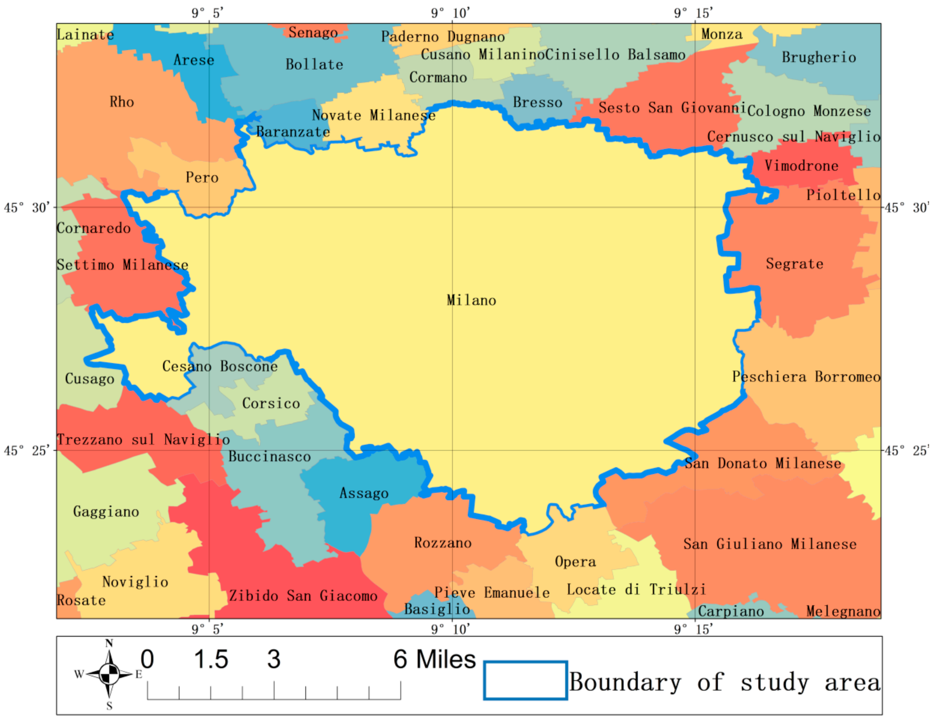
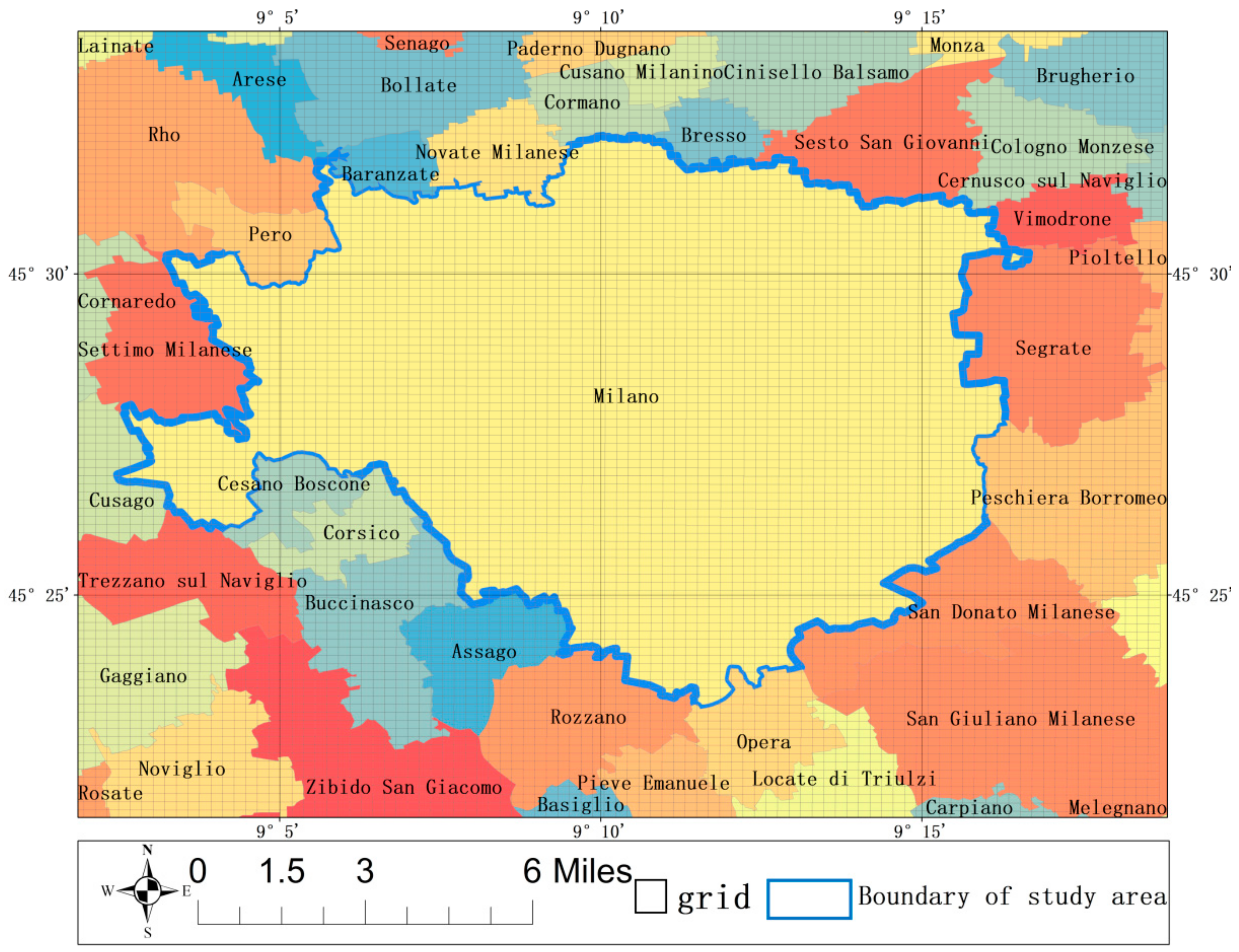
Therefore, the authors propose a spatial hot/cold spot detection method for human communication records by auto-correlating the PageRank ([17] Zhu, 2021) values of spatial interaction networks constructed from the records. The remainder of the article is arranged as follows ([18] Chen et al., 2020): The study area and data are described in Section 2. Section 3 details the proposed methodology. Section 4 presents the results and discussions. Finally, conclusions are presented in Section 5.

2. Study Area and Data

2.1. Study Area

This study was conducted in Milan, which is the second largest city in Italy and a world-famous international metropolis. The city is located in the north of Italy in Lombardy plain (capital of Lombardy region and Milan City), with a permanent population of about 1.47 million and an area of about 181 square kilometers. The GDP of the Milan metropolitan area accounts for 4.8% of Italy’s GDP. In addition, the city is the most densely populated and industrially developed area in Europe. Figure 1 shows the geography of the study area. The authors used two types of experimental datasets: the telephone dataset and the related geographical features dataset.

2.2. Telephone Dataset

The telephone dataset was provided by the first edition of the Big Data Challenge, launched by Telecom Italia (https://dandelion.eu/datamine/open-big-data/, 18 November 2019). The experimental telephone dataset was collected during a week (1–7 November 2007) and spatially aggregated into a non-overlapping spatial tessellation with 10,000 grids, each grid with dimensions of 235 m by 235 m. The overlay map between the grids and the study area is shown in Figure 2.

In addition, the telephone datasets were aggregated over a 10-min period. Finally, through spatial aggregation and temporal aggregation of telephone datasets, spatial interaction could be achieved within 10 min for each pair of spatial grids.

Table 1. Examples of the spatial interaction records.

Square Id1	Square Id2	Time Interval	Directional Interaction Strength
1066	1281	1388579400000	$7.573166813008205 \times {10}^{-4}$
1066	1282	1388595000000	$9.882422919705961 \times {10}^{-5}$
1066	1318	1388530800000	$2.3905419639970557 \times {10}^{-6}$
…	…	…	…

shows examples of the spatial interactive data.

In the table, Square Id1 and Square Id2 are the IDs of the interactive source grid and target grid, respectively. For time intervals, the start time of the interval is expressed as the number of milliseconds that had passed since the UNIX epoch of UTC on 1 January 1970, and the end of the interval can be obtained by adding 600,000 milliseconds (10 min) to this value. The directional interaction strength represents the directional interaction strength between Square Id1 and Square Id2. This value is proportional to the number of calls exchanged between callers in square Id1 and receivers in Square Id2. Overall, the telephone dataset was aggregated into 6,404,487,297 spatial interaction records between 10,000 grids.

2.3. Geographical Features Dataset

The geographic features dataset used in this study mainly includes the land-use dataset and the point-of-interest (POI) dataset ([19] Wu et al., 2018; [20] Li et al., 2019). The land-use dataset was collected by earth observation satellites and combined with observations from the earth’s surface sensor network in 2012. Copernicus is a European program for monitoring the earth (https://land.copernicus.eu/local/urban-atlas/urban-atlas-2012?tab=download, 12 January 2021). The land-use dataset includes 21 land-use types, which is shown in Figure 3.

The point-of-interest (POI) dataset was derived from OSM (https://github.com/openstreetmap, 12 January 2021). It can be divided into eight categories: transportation services, leisure, business, public services, catering and accommodation, party and government organs, sightseeing, and shopping. The overlay map between the POI dataset and the grids is shown in Figure 4.

3. Research Method

The proposed method includes four phases: we used the aggregated telephone dataset to construct a spatial interaction network, and then calculated the PageRank value of each node of the constructed spatial interaction network; secondly, we performed hot/cold spot detection by the PageRank value of the autocorrelated nodes; and finally we performed overlay and statistical analysis on the detected hot and cold maps with the land feature set and POI dataset.

3.1. Construction of Spatial Interaction Network

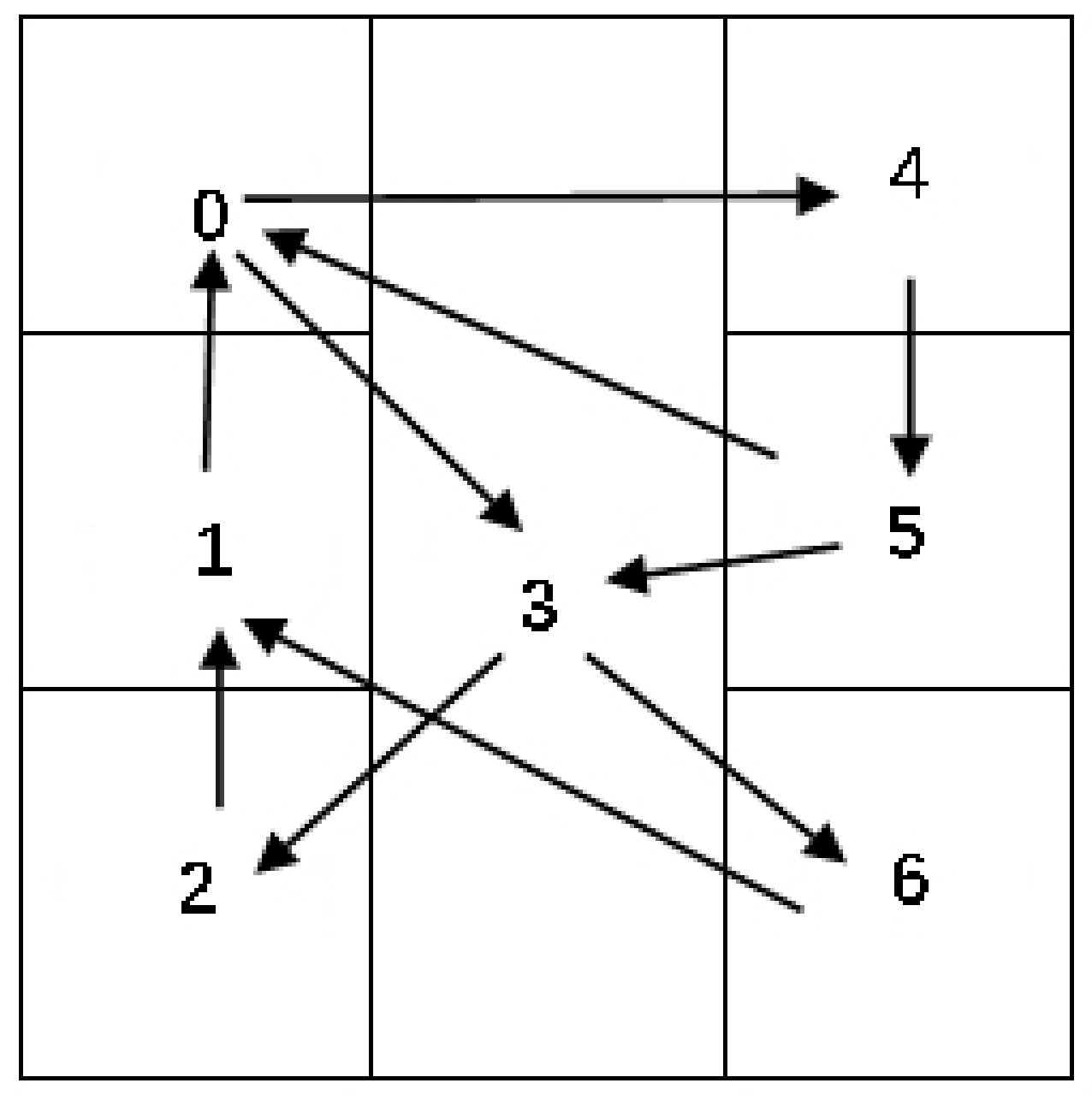
The spatial interaction network is constructed from the records of spatial interaction, which were aggregated from the telephone dataset. The nodes of the network represent grids, and the edges encode calls flows between pairs of grids. The edge is directed and weighted, and the weight of the edge is proportional to the directional interaction strength between the node corresponding to the origin grid and the node corresponding to the destination grid. In addition, the loop edges from locations to themselves are also considered. This process involves two basic definitions.

Definition 1.

Given a non-overlapping spatial tessellation$Grids=\left\{g_1,g_2,g_3,\dots ,g_n\right\}$, where$g_i,1\le i\le n$represents a grid, a spatial interaction record is defined as$SI=\left(ori\_grid,des\_grid, interval, intensity\right)$;$ori\_grid,des\_grid\in Grids$represents the origin grid and the destination grid of the spatial interaction,$interval$represents the temporal aggregation interval of the telephone dataset between the two grids, and$\mathrm{intensity}$represents the directional interaction strength between the two grids.

Definition 2.

Given a set of spatial interaction records$SIs=\left\{s{i}_1,s{i}_2,s{i}_3,\dots ,s{i}_n\right\}$and a non-overlapping spatial tessellation$Grids=\left\{g_1,g_2,g_3,\dots ,g_m\right\}$,$SIN=\left\{V,E\right\}$is defined as a spatial interaction network, where$V=\left\{v_1,v_2,\dots ,v_s\right\},v_i·grid\in Grids,1\le i\le s$; that is, for each node$v_i\in V$, there is a corresponding grid$v_i·grid\in Grids$;$E=\left\{e_1,e_2,\dots ,e_t\right\}, 1\le j\le \left(m\ast \left(m-1\right)\right)$, and the condition is satisfied that for any directed edge$e=\left\{v_o,v_p\right\}\in E$, there is a spatial interaction record$si\in SIs$,$si·origrid=v_o·grid$and$si·desgrid=v_p·grid$.

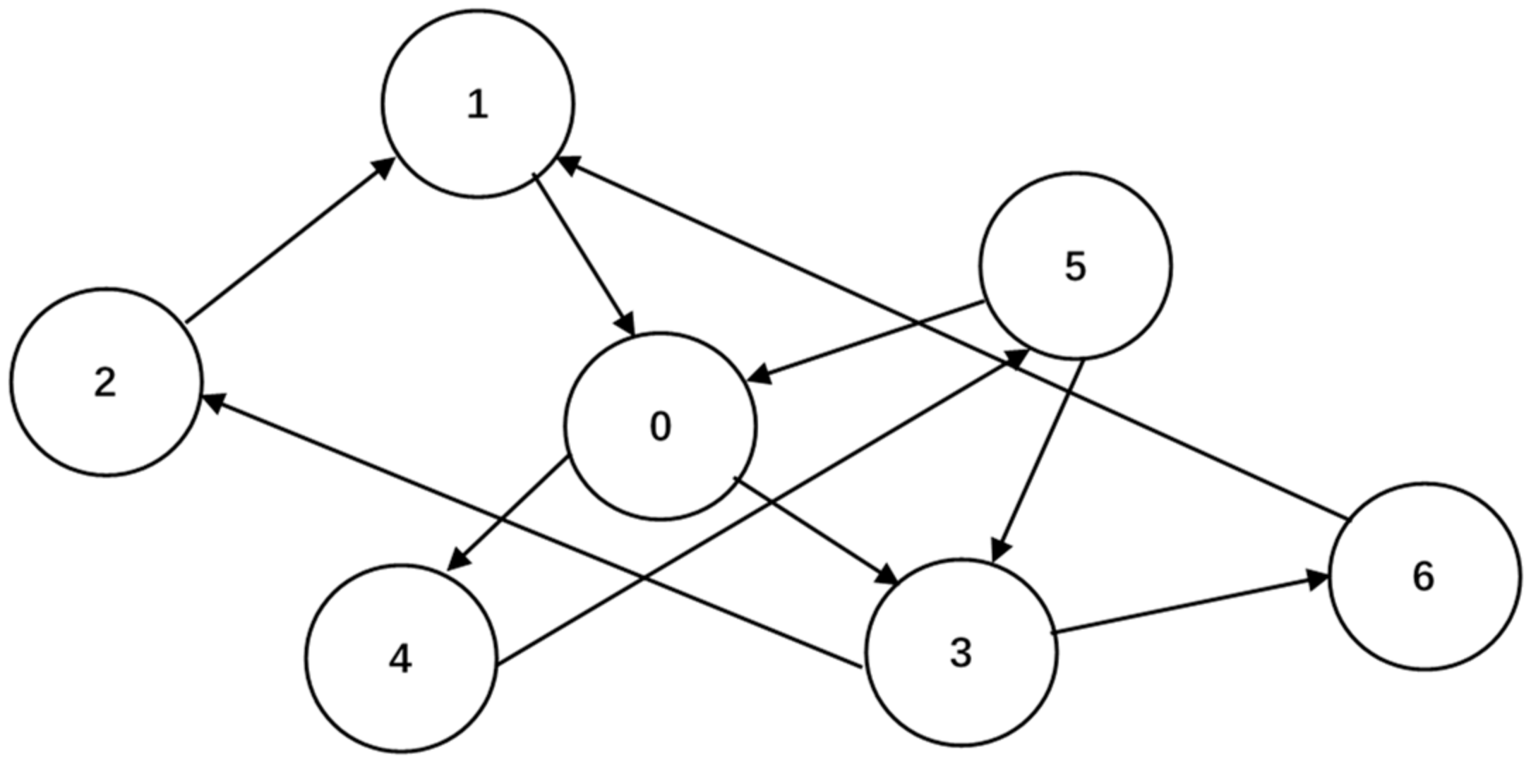
For example, in Figure 5, there are 11 spatial interaction records in a non-overlapping spatial tessellation with 7 grids. The corresponding extracted spatial interaction network is shown in Figure 6.

3.2. Calculation of PageRank Value

PageRank value is originated to evaluate the importance ranking between web pages. In particular, the importance of a page is determined by the number of pages linked to it. A page with more links will have higher importance, that is, higher PageRank value. In this study, we used the PageRank values of the nodes in the spatial interaction network to obtain the interaction between regions with large spatial distance. Unlike simple network features, such as in degree and out degree, PageRank value can reflect the interaction between regions with large spatial distance as the value records the multi-level connection relationship of network nodes. Given a spatial interaction network $\mathrm{SIN}=\left\{V,E\right\}$, the PageRank value calculation formula for the node $v_i\in V$ is:

$$PR\left(v_i\right)=\mathsf{\alpha }{\displaystyle \sum }_{v_j\in M_{v_i}}\frac{PR\left(v_j\right)}{L\left(v_j\right)}+\frac{\left(1-\mathsf{\alpha }\right)}{n}$$

where $M_{v_i}$ represents the set of neighbor nodes directly connected with node $v_i$; $L\left(v_j\right)$ represents the set of neighbor nodes directly connected from the node $v_j$;$PR\left(v_j\right)$ represents the PageRank value of node $v_j$; $n$ is the total number of nodes in $V$; and 𝛼 represents the damping coefficient, which is generally taken as 0.85.

As the experimental spatial interactive data records (about 6.4 billion records) are large, the spatial network generation and calculation of PageRank value can be implemented under the big data computing platform, such as the spark platform ([21] Zhang et al., 2020). The specific code is as follows:

3.3. Detection of Hot/Cold Spots

The idea of hot/cold spot detection is to auto-correlate the PageRank values of nodes of the spatial interaction network constructed from the records. This process involves the definition as follows.

Definition 3.

Given a spatial interaction network$SIN=\left\{V,E\right\}$,$V=\left\{v_1,v_2,\dots ,v_n\right\},$and the set of PageRank values of$V PageRanks=\left\{PR\left(v_1\right),PR\left(v_2\right),\dots ,PR\left(v_n\right)\right\}$, the hot/cold value of node$z_i$is calculated by$G^{\ast }$statistic ([22] Wang et al., 2018; [23] Feng et al., 2018). The formula is:

$$z_i=\frac{PR\left(v_i\right)-\overline{x}}{S^2}{\displaystyle \sum }_j^m{w}_{i,j}\left(PR\left(v_j\right)-\overline{x}\right),$$

where$PR\left(v_i\right)$represents the PageRank value of node$v_i$;$\overline{x}$=$\frac{{{\displaystyle \sum }}_{k=1}^{n}PR\left(v_k\right)}{n}$which represents the mean of PageRank values in$PageRanks$;$S^2=\frac{1}{n}{\displaystyle \sum }_{i=1}^n{\left(PR\left(v_i\right)-\overline{x}\right)}^2$represents the variance of PageRank values in$PageRanks$;$m$represents the number of neighbor nodes directly connected from node$v_i$;$PR\left(v_j\right)$represents the PageRank value of the neighbor node$v_j$; and$w_{i,j}$represents the spatial weight between the node$v_i$and its neighboring node$v_j$.

If $z_i<0$, the grid corresponding to node $v_i$ locates a cold-spot region; if $z_i>0$, the grid corresponding to node $v_i$ locates a hot-spot region. In addition, if $z_i$ = 0, the PageRank value of the node $v_i$ is a random value, and the grid corresponding to node $v_i$ is neither a cold spot nor a hot spot.

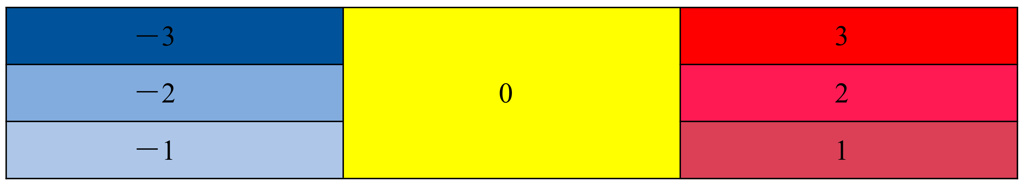
Typically, the hot/cold spots are usually divided into three categories according to the confidence level of $z_i$ [24 ] Zhou, 2019). The level (+3, −3), (+2, −2), and (+1, −1) represents the hot spots and the cold spots with confidence 99%, 95%, 90%, respectively [25 ] Wen, 2018).

Finally, the authors can obtain a set of hot/cold spots $CH=\left\{c_1,c_2,\dots ,c_n\right\}$,$c_i=\left\{\left(z_1,ge{o}_1\right),\left(z_2,ge{o}_2\right),\dots ,\left(z_n,ge{o}_n\right)\right\},1\le i\le n,$ where $ge{o}_n$ is defined as the location of the grid where the node $v_i$ is located. Figure 7 shows an example of the division of hot/cold spots, where $CH=\left\{c_1,c_2,c_3,c_4,c_5,c_6,c_7\right\}, c_1=\left(-3,ge{o}_1\right), c_2=\left(-2,ge{o}_2\right), c_3=\left(-1,ge{o}_3\right), c_4=\left(0,ge{o}_4\right), c_5=\left(1,ge{o}_5\right), c_6=\left(2,ge{o}_6\right), c_7=\left(3,ge{o}_7\right)$.

3.4. Map Overlay and Statistical Analysis

Through map overlay and statistical analysis, we can decide whether the division of cold and hot spots is reasonable. Specifically, the hot and cold areas should contain completely different types of objects and statistics distribution characteristics. Land type data and POI data are two types of typical feature data, which are closely related to human activities. Therefore, in this study, we choose these two kinds of geographic element data and spatial grid for overlay and data analysis.

Map overlay and statistical analysis of spatial data is a basic function of GIS. According to the geometric type of spatial data, there will be different implementation methods. In this article, the authors used two functions of polygons and points to overlay. Specifically, the authors use the polygon overlay operation to analyze the type and quantity of the land-use dataset intersecting with the grids of hot/cold spots, and calculate the type and number of the POI dataset contained in the grids corresponding to the hot/cold spots using a point operation in a polygon. This process includes four basic definitions.

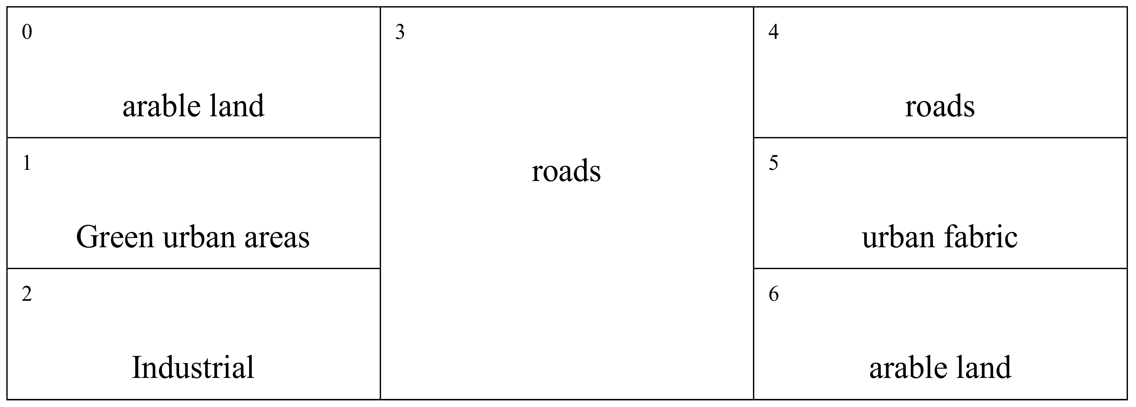
Definition 4.

For a set of land-use types$LandTypes=\left\{l{t}_1,l{t}_2,l{t}_3,\dots ,l{t}_n\right\}$,$GD=\left\{g{d}_0,g{d}_1,g{d}_2,\dots ,g{d}_n\right\}$is defined as a land-use dataset, where$g{d}_i=\left(ge{o}_i,at{t}_i\right),0\le i\le n$is defined as the$i$th element in the geographic dataset,$ge{o}_i$represents the region where the land plot$g{d}_i$is located, and$at{t}_i$represents the land-use type of the land plot$g{d}_i$. For example, Figure 8 includes five land-use types:$arable land,roads,green urban areas, urban fabric,industrial$, and the land-use dataset$GD=\left\{g{d}_0,g{d}_1,g{d}_2,g{d}_3,g{d}_4,g{d}_5,g{d}_6\right\}$, where,$g{d}_0=\left(ge{o}_0,arable land\right),g{d}_1=\left(ge{o}_1,green urban areas\right),g{d}_2=\left(ge{o}_2,industrial\right),g{d}_3=\left(ge{o}_3,roads\right),g{d}_4=\left(ge{o}_4,roads\right),g{d}_5=\left(ge{o}_5,urban frabic \right),and g{d}_6=\left(ge{o}_6,arable land\right)$.

Definition 5.

Given a land-use dataset$GD=\left\{g{d}_1,g{d}_2,\dots ,g{d}_n\right\}$and a set of hot/cold spots$CH=\left\{c_1,c_2,\dots ,c_m\right\}$, where$c_i=\left\{\left(z_1,ge{o}_1\right),\left(z_2,ge{o}_2\right),\dots ,\left(z_s,ge{o}_t\right)\right\},1\le i\le m$, the overlay operation between$CH$and$GD$can be defined as:$C{H}_{GD}=\left\{o{l}_1,o{l}_2,o{l}_3,\dots ,o{l}_m\right\}$, where$o{l}_i=\left\{c_i,polygon\_overlay\left(c_i·geo,g{d}_1.geo\right),polygon\_overlay\left(c_i·grid,g{d}_2.geo\right),\dots ,polygon\_overlay\left(c·geo,g{d}_n.geo\right)\right\},1\le i\le m$. If the intersect topological relationship is satisfied, the$polygon\_overlay$function will return the area where$c_i·geo·$intersects$g{d}_j.geo,1\le j\le n$, and the land-use type$g{d}_j.lt$.

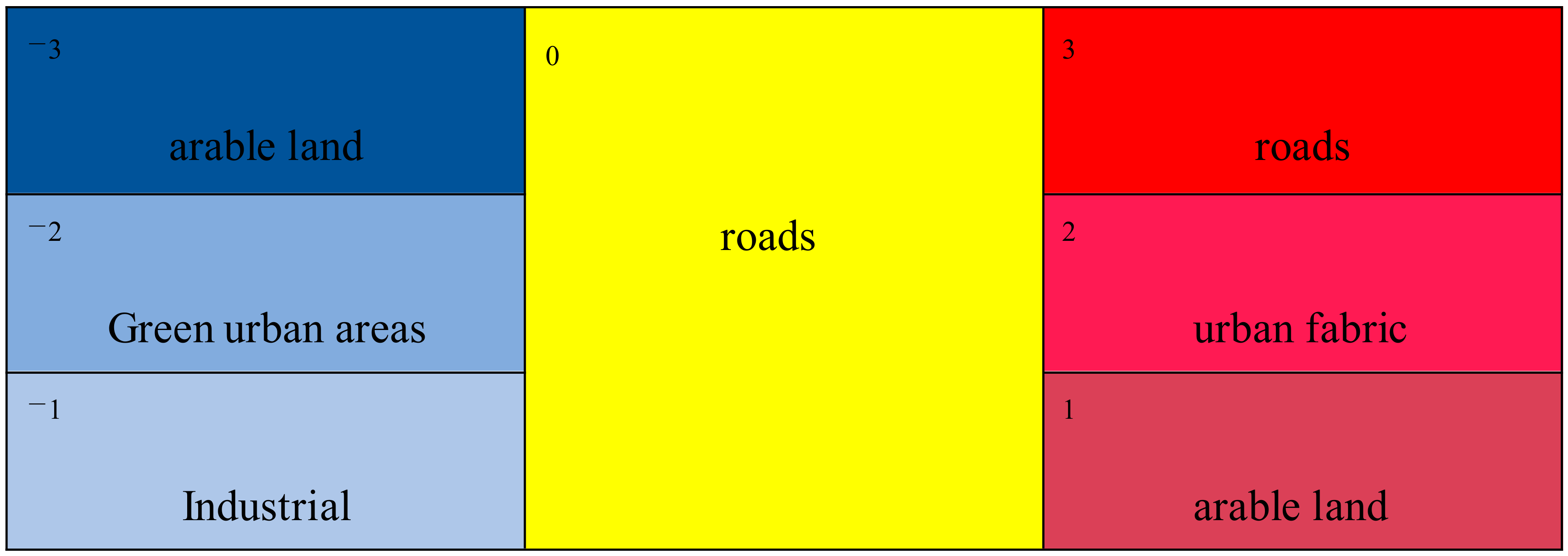
For the hot/cold spots in Figure 7, they overlay with the land-use dataset in Figure 8, and the map overlay result is shown in Figure 9, where $C{H}_{GD}=\left\{\begin{array}{c}\left(\left(-3,ge{o}_0\right),arable land\right),\left(\left(-2,ge{o}_1\right),green urban areas\right),\\ \left(\left(-3,ge{o}_2\right),industrial\right),\left(\left(0,ge{o}_3\right),roads\right),\left(\left(3,ge{o}_4\right),roads\right)\\ \left(\left(2,ge{o}_5\right), urban frabic\right),\left(\left(1,ge{o}_6\right),arable land\right)\end{array}\right\}$.

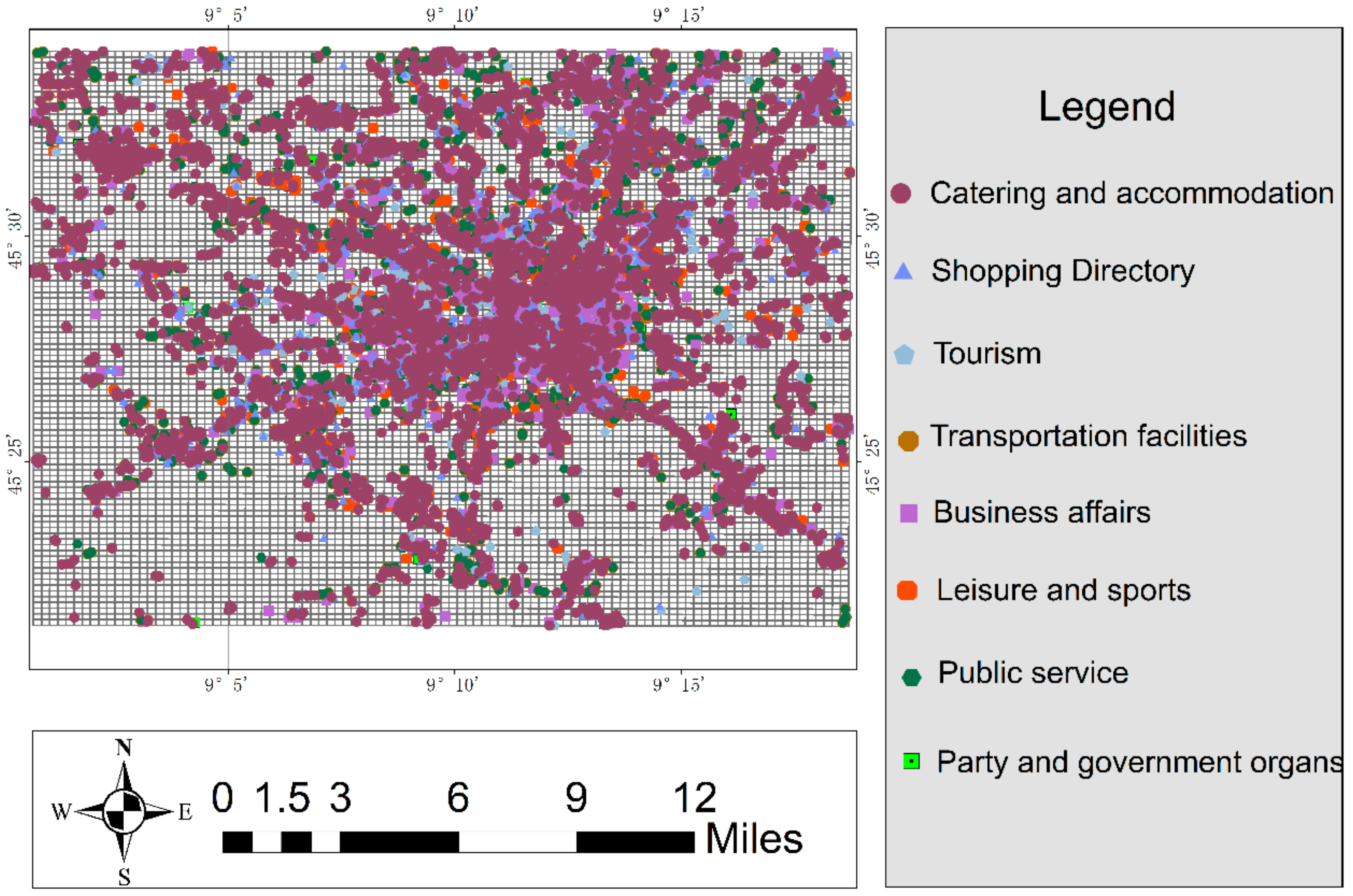
Definition 6.

For a set of POI types$POITypes=\left\{p{t}_1,p{t}_2,p{t}_3,\dots ,p{t}_n\right\}$,$POIdata=\left\{p{d}_1,p{d}_2,p{d}_3,\dots ,p{d}_m\right\}$is defined as a POI dataset, where$p{d}_i=\left(geo,pt\right),0\le i\le m,pt\in POITypes$represents a POI, and$geo$represents the position where the POI is located.

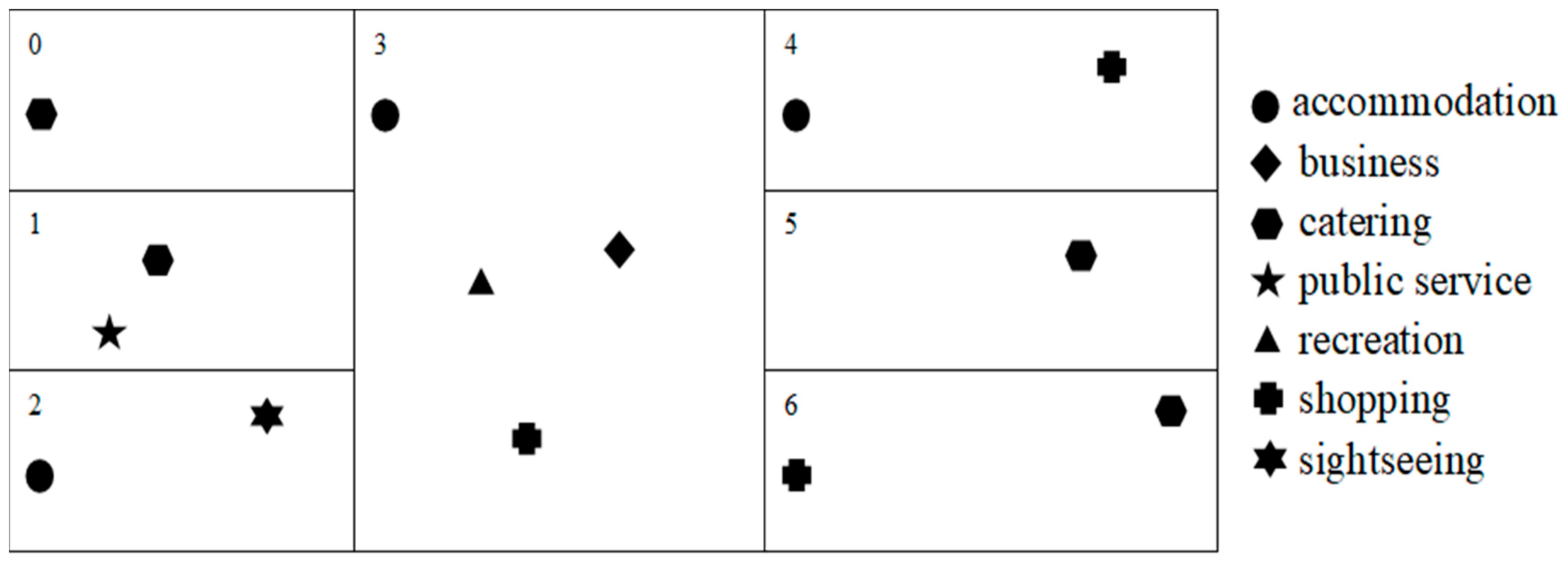
For example, take the POI dataset in Figure 9, which includes seven POI types: $\mathrm{shopping},\mathrm{recreation},\mathrm{sightseeing},\mathrm{catering},\mathrm{business},\mathrm{accommodation},\mathrm{public} \mathrm{service}$. The corresponding POI dataset is: $POIdata=\left\{p{d}_0,p{d}_1,p{d}_2,p{d}_3,p{d}_4,,p{d}_5,p{d}_6\right\}$, where $p{d}_0=\left\{\left(ge{o}_0,catering\right)\right\},p{d}_1=\left\{\left(ge{o}_{1}catering\right),\left(ge{o}_1,public service\right)\right\},p{d}_2=$ $$\begin{gathered} \left\{\left(ge{o}_2,sightseeing\right),\left(ge{o}_2,accommodation\right)\right\},p{d}_3= \\ \left\{\left(ge{o}_3,recation\right),\left(ge{o}_3,accommodation\right),\left(ge{o}_3,business\right),\left(ge{o}_3,shopping\right)\right\},p{d}_4= \end{gathered}$$ $\left\{\left(ge{o}_4,accommodation\right),\left(ge{o}_4,shopping\right)\right\},p{d}_5=\left\{\left(ge{o}_5,catering \right)\right\},p{d}_6=$ $\left\{\left(ge{o}_6,catering\right),\left(ge{o}_6,shopping\right)\right\}$.

Definition 7.

Given a POI dataset$POIData=\left\{p{d}_1,p{d}_2,p{d}_3,\dots ,p{d}_n\right\}$and a set of hot/cold spots$CH=\left\{c_1,c_2,\dots ,c_m\right\},$where$c_i=\left\{\left(z_1,ge{o}_1\right),\left(z_2,ge{o}_2\right),\dots ,\left(z_s,ge{o}_t\right)\right\},1\le i\le m,$the map overlay between$CH$and$POIData$can be defined as$C{H}_{POI}=\left\{o{l}_1,o{l}_2,\dots ,o{l}_m\right\}$, where$$\begin{gathered} o{l}_i=\left\{c_i,point\_in\_polygon\left(c_i· \\ geo,p{d}_1.geo\right),point\_in\_polygon\left(c_i·geo,p{d}_2.geo\right),\dots ,point\_in\_polygon\left(c_i·geo,p{d}_n.geo\right)\right\},1\le i\le m \end{gathered}$$. If the point in the polygon topological relationship is satisfied, the$point\_in\_polygon$function will return the POI type$p{d}_j.lt,1\le j\le n$.

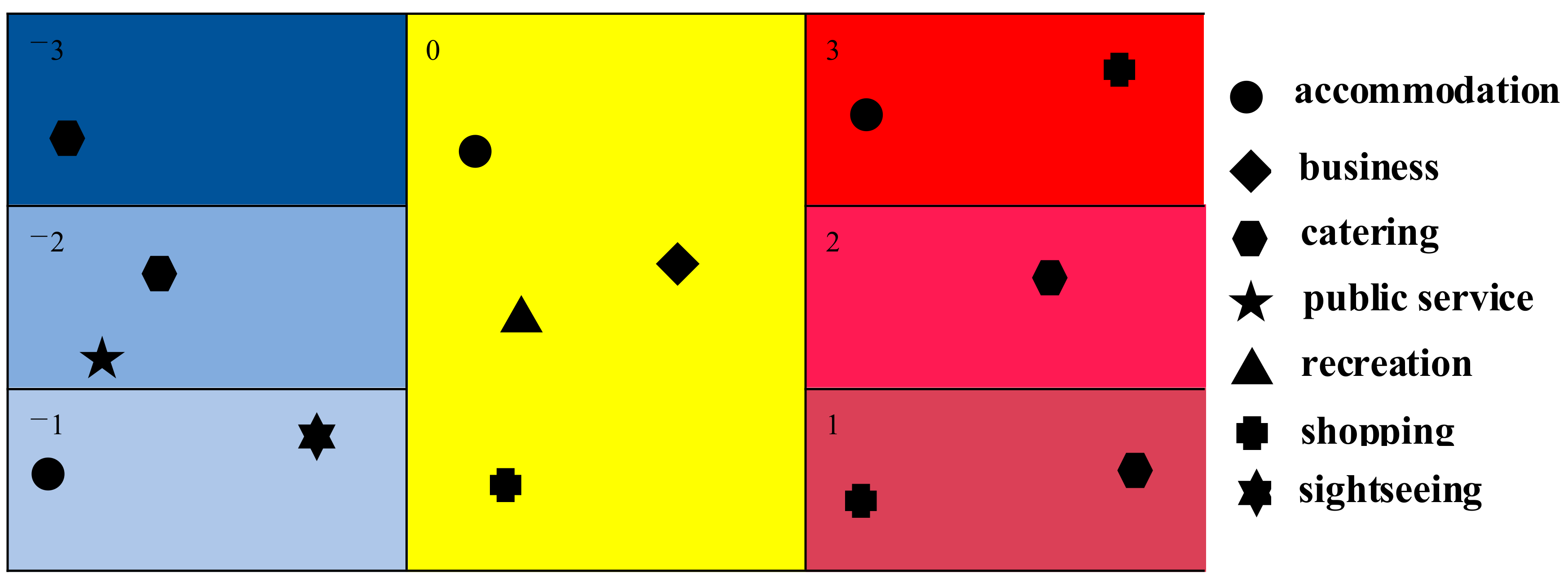
For the classification of hot/cold spots in Figure 7, they overlay with the POI dataset in Figure 10, and the map overlay result is shown as Figure 11, where $C{H}_{POI} \mathrm{is}$

$$\left\{\begin{array}{c}\left(\left(-3,ge{o}_0\right),catering\right),\left(\left(-2,ge{o}_1\right),catering\right),\\ \left(\left(-2,ge{o}_1\right),public service\right),\left(\left(-1,ge{o}_2\right),accommodation\right),\\ \left(\left(-1,ge{o}_2\right),sightseeing\right),\left(\left(0,ge{o}_3\right),accommodation\right),\left(\left(0,ge{o}_3\right),recation\right),\\ \left(\left(0,ge{o}_3\right),business\right),\left(\left(0,ge{o}_3\right),shopping\right),\\ \left(\left(3,ge{o}_4\right),accommodation\right),\left(\left(3,ge{o}_4\right),shopping \right),\left(\left(2,ge{o}_5\right),catering \right),\\ \left(\left(1,ge{o}_6\right),catering \right),\left(\left(1,ge{o}_6\right),shopping\right)\end{array}\right\}$$

4. Experiments and Discussions

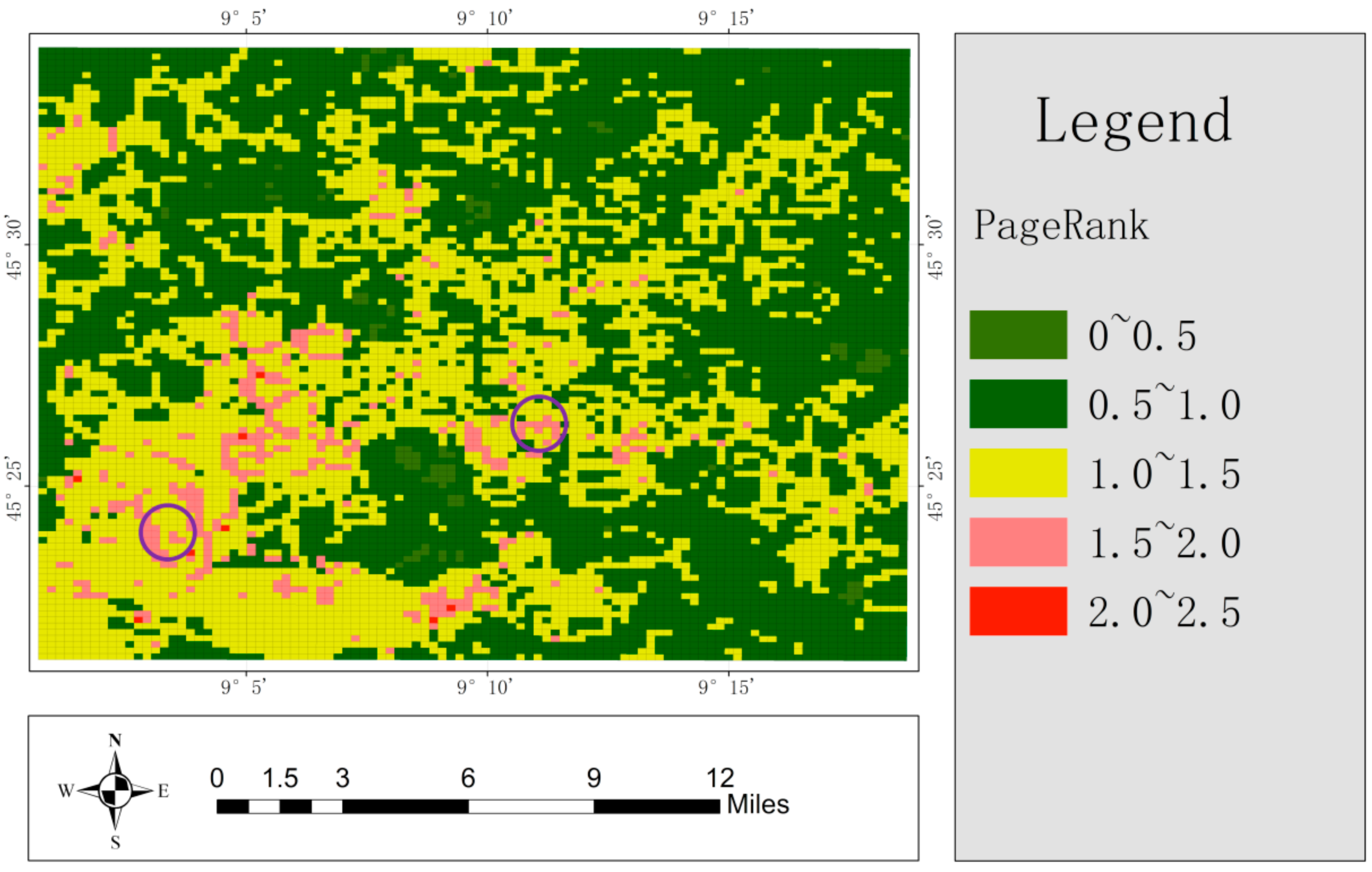
The experimental spatial interaction records were collected from November 1 to 7 in 2013, and one aggregation network was constructed, which included 10,000 nodes and 1,169,475,402 edges. For each node in the network, the authors used the Algorithm 1 to calculate its PageRank value. Based on the corresponding grids of the nodes, the thematic map of nodes PageRank values were obtained, as shown in Figure 12.

Algorithm 1 NetworkGen_PageRank (SIFile, ref Graph)

Input: SIFile represents the spatial interaction records file.

Output: Graph represents the generated spatial interaction network.

(1) val phonedata = sc.textFile(path + recorddata)

(2) val edges:RDD[Edge[Int]] = phonedata map {

line ≥

val row = line split “\t”

Edge(row(1).toInt, row(2).toInt,1)

}

(3) val egograph:Graph[Int,Int] = Graph.fromEdges(edges,1)

(4) val uniqueInputGraph = egograph.groupEdges((e1, e2) ⇒ e1 + e2)

(5) val ranks = uniqueInputGraph.pageRank(0.1). vertices

Line 1 reads the communication data phonedata. Lines 2–3 are preliminarily composed to obtain the raw network egograph. The line 4 egograph combines the same edges of the outgoing grid node and the access grid node in all the data records and adds the weights to obtain the constructed network uniqueInputGraph. Line 5 obtains the PageRank values of all the nodes.

As can be seen from Figure 12, there are mainly three colors distributed in a large area: green, yellow, and pink. The green indicates low PageRank value, which represents the near-distance communication data interaction area. By contrast, pink indicates high PageRank value, which represents the long-distance communication data interaction area. Meanwhile, the yellow area is between the green and the pink.

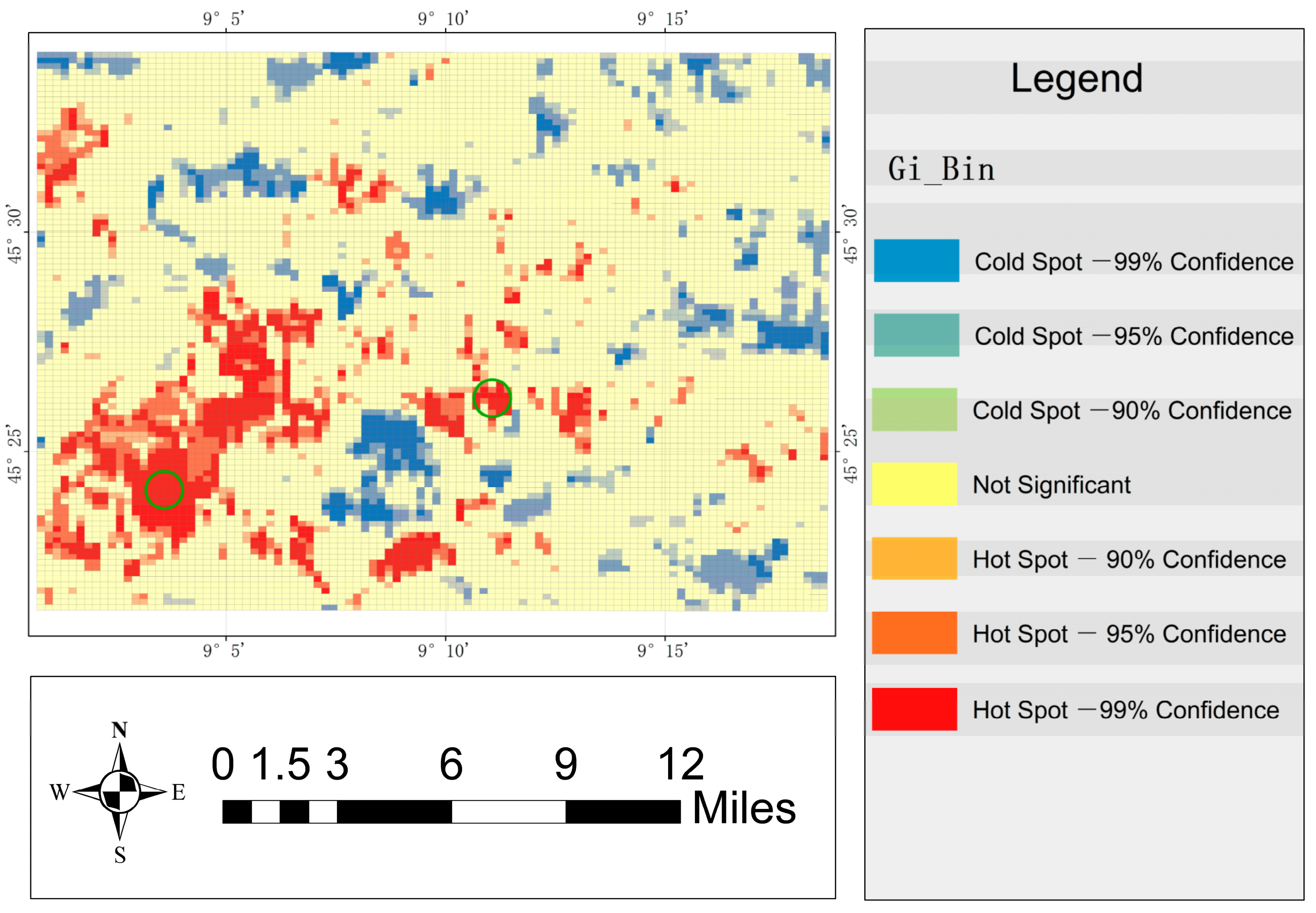
Furthermore, the authors used the detection method proposed in this article to detect the hot/cold spots, and the spatial distribution of the hot/cold spots is shown in Figure 13. It can be seen from the Figure 13 that the detected hot/cold-spot regions are clearly distinguished by their spatial distribution. In particular, the hot spots are mainly distributed in the southwest, while the cold spots are widely distributed. In addition, some grids with long spatial distance (i.e., the pink areas marked by the two purple circles in Figure 12) are also clustered into the same level of hot spots (i.e., the areas marked by the two green circles). The main contribution of the proposed method is to find the regions with long-distance interaction, and then use the clustering method to cluster the regions with long-distance interaction into cold and hot spots at the same level. Then, the authors argued that these results can prove the effectiveness of the proposed method.

(1)

Spatial distribution comparison of geographical features dataset contained by hot/cold spots detected.

The authors applied the map overlay and statistical method proposed in this article to verify whether the hot/cold spots detected are consistent with the real situation of the study area.

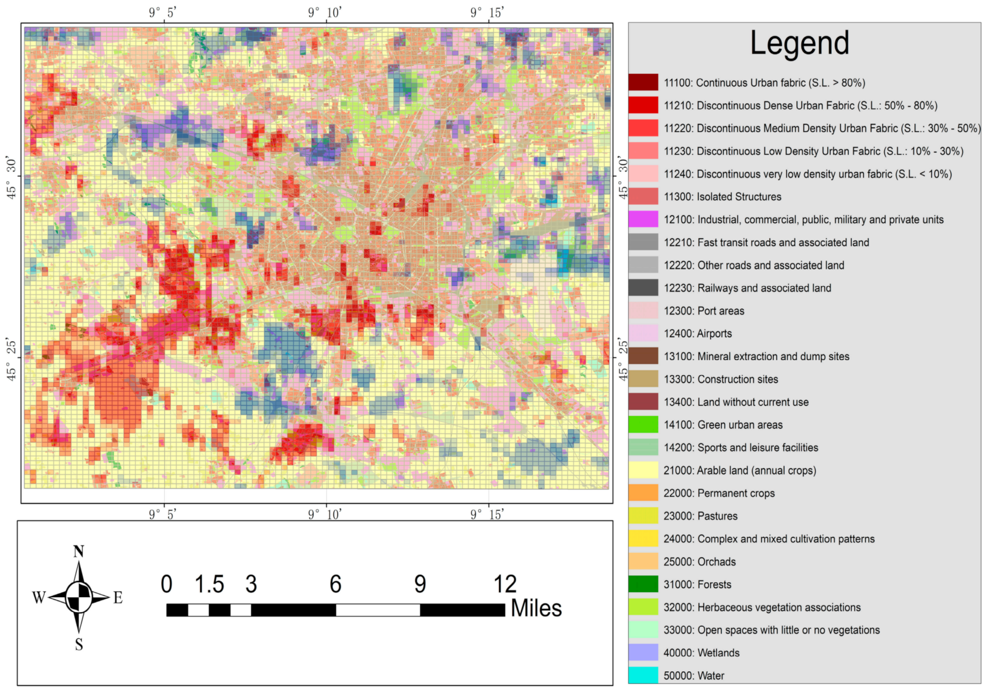
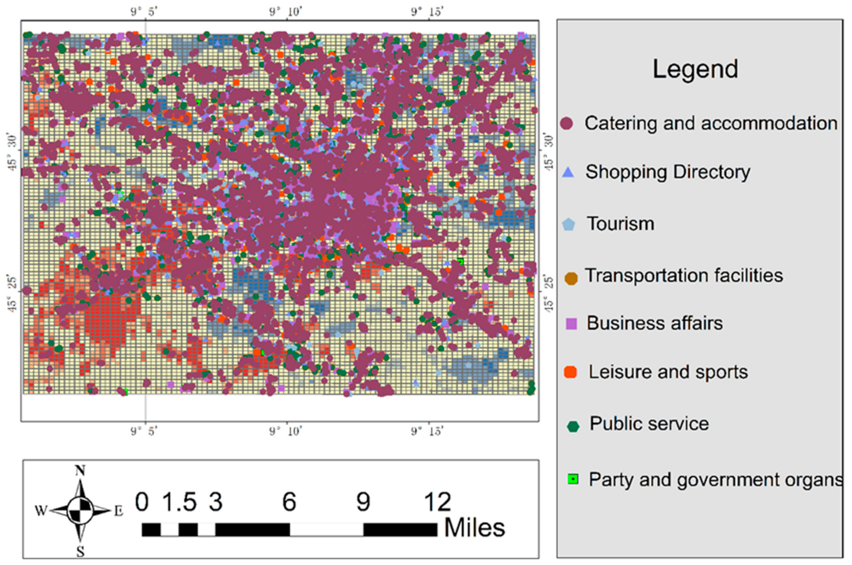
The authors used the map overlay to detect hot/cold spots with the experimental land-use dataset and the POI dataset, and the results are shown in Figure 14 and Figure 15. The authors found through visual interpretation, as shown in Figure 14, that the hot-spot regions contained the two main types of land use, i.e., arable land (annual crops) and other roads, while the cold-spot regions mainly contained arable land (annual crops). In addition, as shown in Figure 15, the authors found that the hot-spot regions contained few types and quantities of POI, i.e., catering and accommodation and transportation facilities, while the cold-spot regions contained more types and quantities of POI. The experimental results are consistent with the real situation of the study area, that is, Milan as a city focusing on the development of transportation, has a perfect large-scale intercity transportation network; therefore, the hot spots area mainly include other roads and transportation facilities, and both industrial land and urban areas with high population density rely on transportation. Therefore, POIs are scattered near transportation lines.

However, the relationship through spatial visualization analysis between the hot/cold regions and geographic features obtained was not accurate enough, so the authors further conducted a quantitative statistical analysis. The quantitative statistical analysis included two comparisons: quantity distribution comparison and ratio distribution comparison.

(2)

Quantity distribution comparison of geographical features dataset contained by hot/cold spots detected.

The authors performed the quantity distribution comparison of the land-use dataset contained by the hot/cold spots detected from spatial interaction network constructed from the telephone records in Milan city. The result is shown in Figure 16.

As can be seen from Figure 16, whether it is a cold spot or a hot spot, the two types of land-use dataset, arable land (annual crops) and other roads and associated land, have a large grid number. The reason is that the southern part of Milan city focuses on the development of agriculture and transportation systems. Then, to make a more accurate analysis, the authors eliminated these two types of land-use datasets, and compared only other types of land-use datasets in the coldest/hottest regions. The results are shown in Figure 17.

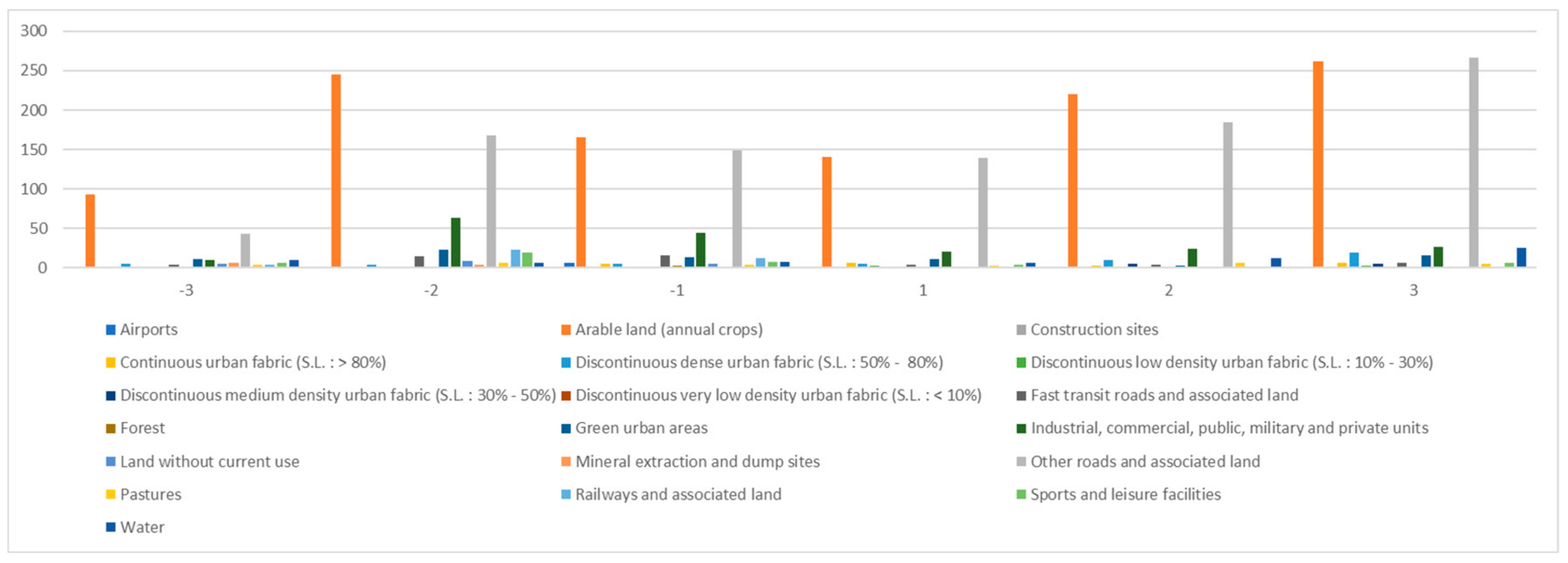
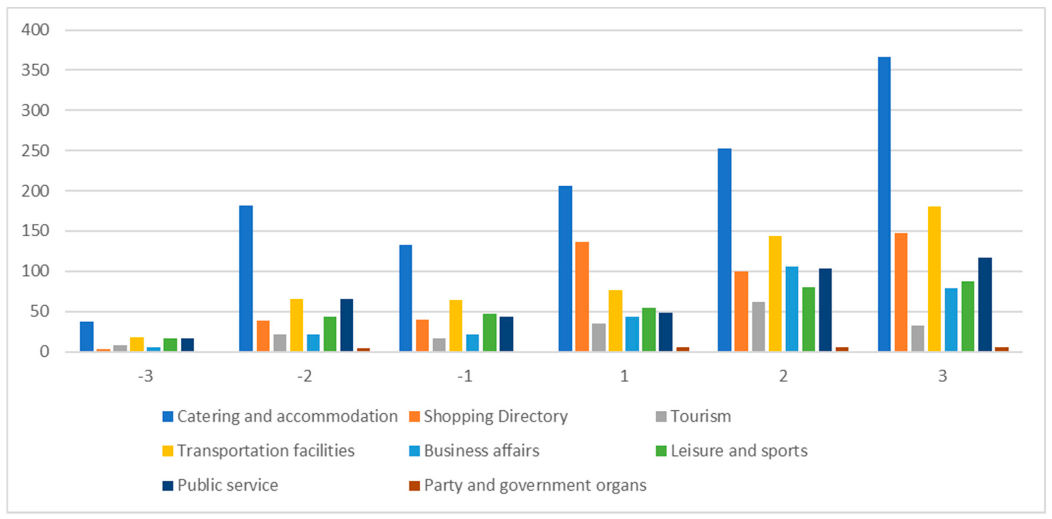
The authors can see from Figure 17 that there are more types of land-use datasets in the cold-spot regions than in the hot-spot regions, but in the hot-spot regions, the grid number of land-use datasets (i.e., discontinuous dense urban fabric (SL: 50–80%); industrial, commercial, public, military and private units; green urban areas; water) is significantly greater than the grid number in the cold-spot regions. In addition, the authors performed the quantity distribution comparison of the POI dataset contained by the hot/cold spots detected, and the result is shown in Figure 18. It can be seen from Figure 18 that the types and numbers of the POI dataset in hot spots are significantly more than those in cold spots. Therefore, the experimental results are consistent with the real situation; compared with the cold-spot regions, hot-spot regions require more infrastructure services because of the intensive human activities. That is, more land use data and POI data need to be included.

It will be more clear to use the number of grids to present the results, but if the number of grids in each category is different, it is not suitable for comparing the number, so we will use the ratio to present the results.

(3)

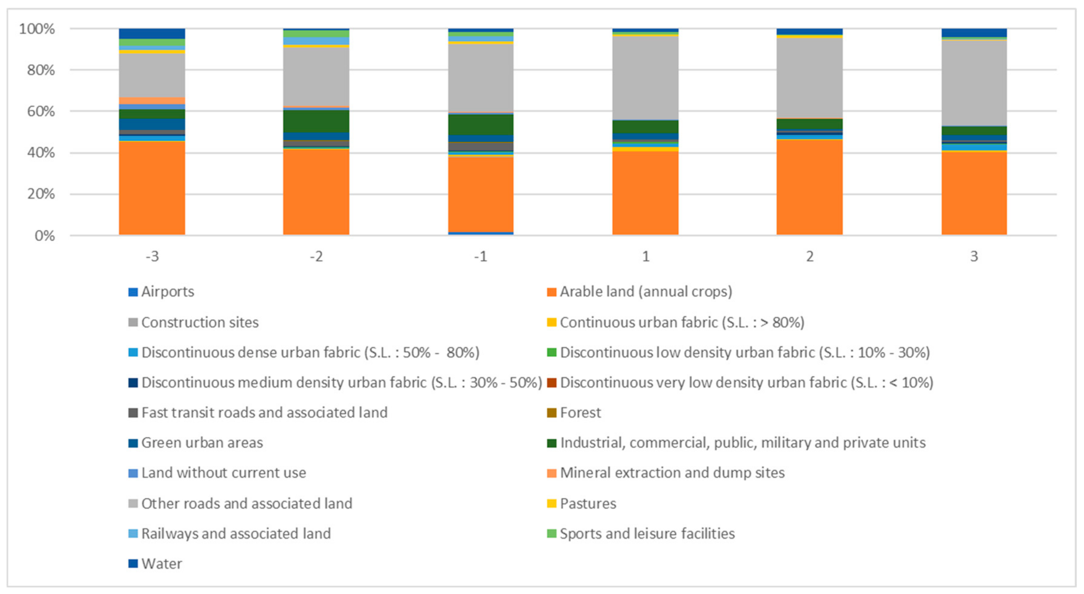
Ratio distribution comparison of geographical features dataset contained by hot/cold spots detected.

As the number of geographical features contained depends on the area of hot/cold regions, the authors further experimented to compare the ratios of types of geographical features contained in the hot/cold regions. Relative entropy, also known as Kullback Leibler divergence or information divergence, is an asymmetric measure of the difference between two probability distributions. In information theory, the relative entropy is equivalent to the difference of the information entropy of two probability distributions. In order to clearly express the difference between hot spots and cold spots, this study uses the method of relative entropy. The specific formula is as follows:

$$relative entropy={\displaystyle \sum }_{i=1}^{n}rati{o}_{p\left(i\right)}\ast log\frac{rati{o}_{p\left(i\right)}}{rati{o}_{q\left(i\right)}}$$

The ratio comparison of the land use dataset contained by hot/cold spots detected is shown in Figure 19.

The authors calculated the relative entropy values between −3 and 3, −2 and 2, −1 and 1, and the results are 1.019, 1.035 and 1.033, respectively. These values indicate the ratio values of the land use dataset contained by hot spots and cold spots are slightly different. The reason is that the ratio values of arable land (annual crops) and other roads and associated land are much larger than that of other types of values. 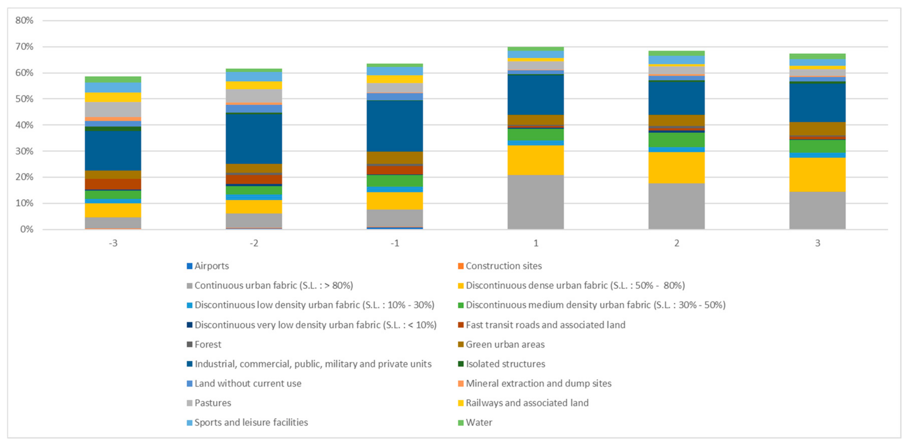Therefore, to ensure the effectiveness of data analysis, the authors removed these two types of values, and the results are shown in Figure 20.

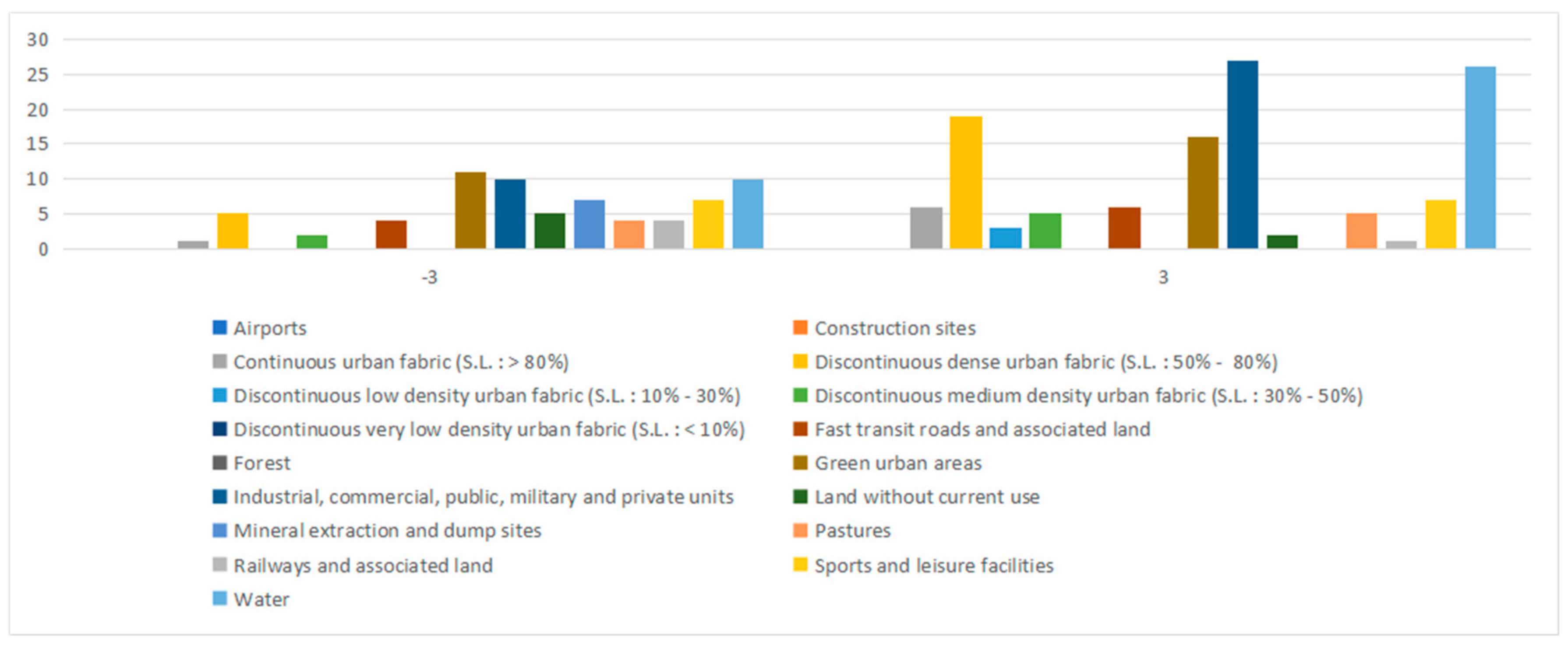
As can be seen in Figure 20, industrial, commercial, public, military, and private units account for a larger proportion of different levels of cold and hot spots, and the proportion in the hot-spot areas is larger than that in the cold-spot area. The relative entropy values between −3 and 3, −2 and 2, −1 and 1 are 0.595, 0.609 and 0.638 respectively, which further verifies that the land type area in cold-spot area and that in hot-spot area are significantly different.

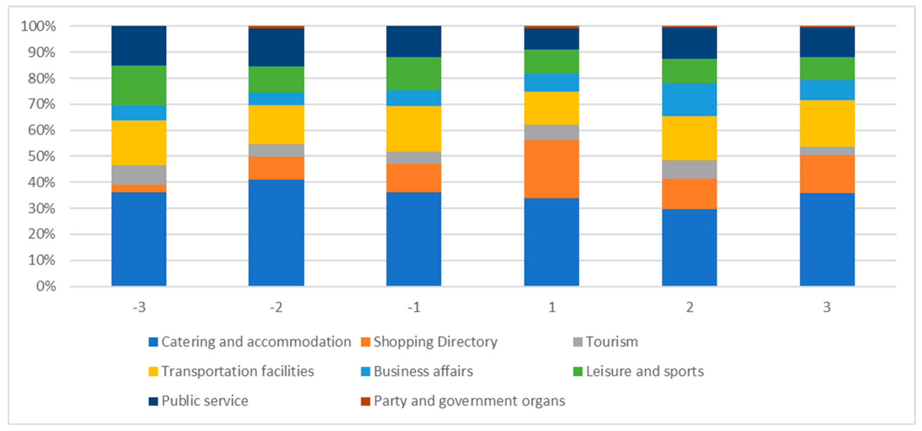
Similarly, the authors further experimented to compare the ratios of types of the POI dataset contained in the hot/cold regions. The results are shown in Figure 21. The authors can see that for shopping directory and business affairs, the proportion of hot spots is significantly greater than that of cold spots, while for leisure, sports, and public service, the opposite is true. The relative entropy is 0.959, 0.925, and 0.973, respectively. It can be seen that there are some differences between cold-spot region and hot-spot region in the distribution area of POI. The distribution ratio of POI in the cold-spot area is relatively consistent, while the distribution ratio of POI in the hot-spot area fluctuates to some extent. The ratio of POI in the hot-spot area is also slightly greater than that in the cold-spot area. Thus, the experimental results are consistent with the real situation that people are mainly engaged in industrial and commercial activities in the hot-spot regions, while people in cold-spot regions are mainly engaged in leisure and entertainment activities.

5. Conclusions

As the existing methods for detecting hot/cold spot cannot apply the datasets (i.e., human communication records) generated from interactions between larger spatial regions, the authors proposed a novel method. This method detects spatial hot/cold spots by auto-correlating the PageRank values of spatial interaction networks constructed from the records. The authors performed extensive experiments to verity the proposed method. The authors selected Milan, Italy as the study area, and the spatial interaction records reflected by the telephone calls, the land-use dataset, and the POI dataset as the experimental dataset. The experimental results indicate the following. (1) The proposed hot/cold spot detection method can apply to the long-distance spatial interactive recording data. Specifically, some grids with long spatial distance also clustered the same level of cold spots or hot spots. (2) The detected hot/cold-spot regions are clearly distinguished by the statistical distribution (i.e., spatial distribution, quantity distribution, and ratio distribution) of the containing land-use dataset and the POI dataset. In particular, in terms of spatial distribution: the hot spots were mainly distributed in the southwest of Milan city, while the cold spots were widely distributed. In addition, in terms of quantity distribution and ratio distribution: the grid number of hot spots was greater than the grid number of cold spots. (3) These distribution differences of hot/cold spots are in line with the real situation of the study area, according to interpretation and analysis, specifically, the statistical distribution differences (i.e., spatial distribution, quantity distribution, and ratio distribution) of the containing land-use dataset and the POI dataset in hot/cold spots. In summary, the comprehensive experimental results prove the correctness of our proposed method.