A Novel Traffic Flow Reduction Method Based on Incomplete Vehicle History Spatio-Temporal Trajectory Data

Abstract

In order to improve the effect of path planning in emergencies, the missing position imputation and velocity restoration in vehicle trajectory provide data support for emergency path planning and analysis. At present, there are many methods to fill in the missing trajectory information, but they basically restore the missing trajectory after analyzing a large number of datasets. However, the trajectory reduction method with few training sets needs to be further explored. For this purpose, a novel trajectory data cube model (TDC) is designed to store time, position, and velocity information hierarchically in the trajectory data. Based on this model, three trajectory Hierarchical Trace-Back algorithms HTB-p, HTB-v, and HTB-KF are proposed in this paper. Finally, experiments verify that conduct in a different number of sample sets, it has a satisfactory performance on information restoration of individual points of the trajectory and information restoration of trajectory segments.

1. Introduction

The intelligent transportation system has become hot in recent years, many approaches on intelligent transportation have been proposed as a result. The excavation of flow can be used to support vehicle traffic planning [1,2], vehicle path recommendation [3,4], subway station location planning [5,6], vehicle emergency management [7,8], etc. The potential commercial value can be obtained through the analysis of vehicle trajectory [9,10]. At present, there are various analysis methods for vehicle trajectory. For example, through the historical trajectory data of vehicles, the prediction of urban traffic flow, the mining of interest points in the city, the prediction of the launching points of shared bikes, and even the planning of urban public transport service points through the analysis of taxi trajectory density and stop point detection.

The analysis of vehicle trajectory helps to analyze the travel pattern of citizens, etc. Tang et al. [11] analyzed the car pooling travel patterns of passengers in that develop a Prefixspan-prediction using a partial matching (P-PPM) target prediction algorithm to mine frequent motion patterns from trajectory data and determine the confidence of motion rules. The method takes the total travel time as the matching target. Zhou et al. [12] studied of the trajectory of the context information and the found extract information such as location information is through an analysis of the first to verify the knowledge, however, mobility management is an important problem is how to learn an accurate travel itinerary, so they proposed a trajectory of the encoder and decoder trip recommended method. This is a novel end-to-end approach that encodes historical trajectories as vectors while capturing the inherent characteristics of individual Point of Interest (POI) and the transformation patterns between POIs. The historical attention mechanism is incorporated into the sequential to sequential trip recommendation task of the method to improve effectiveness. Zou et al. [13] proposed a geographic services recommendation model (GSRM), which roughly consists of three basic steps. First, the position sequence is obtained by clustering GPS positions. To improve efficiency, we adopt a programming model with distributed algorithm to accelerate clustering. Secondly, the position sequence to mine spatial and temporal information from cluster trajectories. The MiningMP algorithm is designed that the next possible location the user will travel to is predicted. A comprehensive framework can then be constructed for GSRM and provide appropriate geographic recommendation services by taking into account location information. The MiningMP algorithm provide appropriate geographic recommendation services by considering location sequences and other relevant semantic information.

The prediction of traffic flow can assist in directing traffic flow and other issues. Li et al. [14] proposed a novel multi-sensor data correlation graph convolutional network model (MDCGCN). The MDCGCN model is composed of near-term, daily and weekly periods, and each part is composed of two parts: (1) reference adaptive mechanism and (2) multi-sensor data correlation convolution block. The first part can eliminate the differences between periodic data and effectively improve the quality of data input. The second part can effectively capture the dynamic temporal and spatial correlation caused by the change of traffic mode relationship between roads. Hou et al. [15] studied short-term traffic flow prediction model that a novel cloud-edge-IOT three-layer traffic flow edge computing architecture and a short-term traffic flow prediction method based on spatio-temporal correlation is proposed, which uses principal component analysis (PCA) to analyze intersection correlation. Convolutional gated recurrent unit (CONVL-GRU) and Bidirectional GRU (Bi-GRU) are used to extract the spatio-temporal and periodic characteristics of traffic flows. You et al. [16] proposed an improved cellular automata (CA) model to reveal prediction of traffic flow at signalized intersections. Traffic density and average speed are calculated to study the characteristics and spatial evolution of traffic flow at signalized intersections based on CA model. On this basis, a new traffic rule control optimization model and a CA model with self-organizing traffic signal system is proposed. Sunflower cat optimization (SCO) algorithm was used to predict the flow effectively. The algorithm is designed by combining sunflower optimization algorithm (SFO) with cat swarm optimization algorithm (CSO). In addition, fitness function is designed to guide the control rules of CA model traffic simulation evaluation.

To sum up, the above studies are dependent on the accuracy of trajectory data. However, due to signal shielding or other reasons, a large number of trajectory points are often lost or discontinuous trajectory segments appear in the trajectory. Therefore, we will build a Trajectory Data Cube model (TDC) $\Psi${$t_n$, $p_n$, $v_n$} to store the trajectory data of taxis, and restore vehicle driving conditions at every moment in the road network through hierarchical compression method, where $t_n$ is time, $p_n$ stands vehicle position, and $v_n$ represents vehicle velocity. A Hierarchical Trace-Back method (HTB) will be designed based on taxi historical trajectory to study the restoration of lost trajectory and missing information. Due to the particularity of taxi, its trajectory data are basically in the road network, and taxi can provide a large amount of trajectory data for data analysis.

Table 1. Notations.

Notation	Definition
$\Psi$	represents trajectory information
$t_n$	is $time$ expression
$p_n$	is $position$ expression
$v_n$	represents $velocity$ expression
a	represents the acceleration of two points
$pos$	is trajectory point position information
$vel$	represents trajectory point velocity information
$time$	is trajectory point time-stamp
$Tra<T,P>$	represents a trajectory expression
$MEE$	is the Mean Euclidean Error between the position
$\varphi$	represents reduction velocity error rate

shows the main parameters mentioned in this paper.

In this paper, the traffic condition at any time in history is obtained by data compression and dilution, so as to integrate the incomplete vehicle trajectory data and provide more accurate help for the analysis of trajectory data. The main contributions of this paper are as follows:

• We build a data cube with spatio-temporal characteristics by analyzing the trajectory data of taxis, store the trajectory data of each day in the cube, and finally merge the multi-day data into a TDC model.
• We analyze the trajectory data of each layer through the established TDC, and compress the data layers by HTB-p, HTB-v, and HTB-KF methods. Gain the traffic condition of the road network at a certain time.
• Finally, the thinning method is used to verify the effect of HTB-p, HTB-v, and HTB-KF methods and real historical road network traffic, and compared with existing traffic condition prediction methods and trajectory completion strategies.

The rest of this paper is organized as follows. Section 2 introduces the traffic flow prediction methods and the completion trajectory strategy. Section 3 presents trajectory data cube model based on incomplete taxi trajectory data. Section 4 introduces a hierarchical track-back algorithm to restore the historical trajectory data of vehicles. Section 5 conducts three experiments to verify our methods and the conclude in Section 6.

2. Literature Review

At present, the more popular methods of vehicle historical trajectory mining technology include trajectory completion method based on context analysis, difference completion method, and use deep learning method to predict trajectory. These methods explain the meaning of trajectory data and explore the pattern of trajectory data from different theoretical perspectives, which lays a foundation for the management and modeling of spatio-temporal data and the discovery of road network knowledge [17].

2.1. Context-Based Vehicle Trajectory Analysis

Analyzing trajectory data based on context information is one of the main methods to process trajectory data in the early stage, which requires a large amount of historical trajectory data information. Zhu et al. [18] studied the trajectory context information and used a clustering method to group the trajectory of a specific period, restoring the road characteristics and predicting the road condition through the similar trajectory obtained. Dai et al. [19] analyzed the missing characteristics of moving trajectory data and accurately located and completed the data through the trajectory data of ground sampling frequency. Considering the economy of sampling equipment, vehicles rarely use equipment with high sampling frequency, so there are many inaccuracies and missing points in trajectory data with low sampling frequency. A context-based uncertainty reduction and ranking (CURR) is designed to deduce missing trajectory points and low precision points. Mousa et al. [20] proposed a dual-device trajectory sampling hardware based on the low sampling frequency and poor accuracy of trajectory data. This hardware complements the trajectory by electrical components and by combining the existing GPS trajectory context data. Jansen et al. [21] proposed a ship trajectory prediction method combining semantic trajectory context information and dynamic Bayesian networks. This method uses Bayesian network to calculate the probability between ship trajectory and sample trajectory to predict ship trajectory. The advantage of this method lies in the probability ranking of different trajectories by probability statistics method, so as to analyze the trajectories of ships and predict their positions at the next time. Ding et al. [22] designed an online two-level vehicle trajectory prediction framework. This method combines high-level policy prediction with low-level context inference. The Long-Short Term Memory (LSTM) network is used to predict driving strategies (e.g., forward, yield, left, right, etc.) using its continuous historical observations. The strategy is then used to guide the low-level optimization process based on context reasoning. Blais et al. [23] deduced drivers’ driving behaviors according to the context information of vehicle trajectory, so as to obtain more vehicle trajectory information individually. Yu et al. [24] proposed a new dynamic and static context-aware attention network (DSCAN). DSCAN uses the attention mechanism to dynamically determine which surrounding vehicles are currently more important. A constraint network is also used to design DSCAN to take static environment information into account.

2.2. The Method of Trajectory Missing Point Completion Based on Interpolation Algorithm

The completion strategy of trajectory data is mainly to complete the missing part of trajectory data through interpolation and other strategies for the breakpoints or missing information contained in trajectory sampling data. Li et al. [25] proposed an interpolation method based on bidirectional unequal interval kernel adaptive filtering to solve the problem of data loss in vehicle test trajectory measurement. The training samples of the adaptive filter are designed according to the data before and after the missing data segment of trajectory measurement. After training, the kernel adaptive filter is used to predict the missing data bidirectional. Cruz et al. [26] analyzed traffic vehicle trajectory based on real datasets, which proved their sparsity and incompleteness problems and hindered location prediction. In this context, a method to deal with the problem of missing data is proposed. It also discusses how to combine this method with predictors based on recursive neural networks. In particular, precision measures were adjusted to account for missing values in the test set by introducing the distance between the predicted location and the next location registered. Wei et al. [27] proposed a method based on particle filter (PF) to reconstruct vehicle trajectory on signal mainlines using sparse detection data. First, the main road intersections are divided into several road units, and the estimation of unit travel time is transformed into a quadratic programming problem. Then, PF is applied to reconstruct incomplete vehicle trajectory between successive updates. Specifically, in order to calculate and update the initial particle weight, taking into account the structure of the signal trunk line and the characteristics of vehicle renewal, three important sampling measurability criteria were designed, namely travel time adjustment accuracy, trunk connection speed limit and travel time adjustment possibility. Qi et al. [28] studied sparse trajectory reconstruction based on ALPR data. According to the reasonable travel time threshold, the method divides multiple travel activities of vehicles and identifies incomplete vehicle trajectory. Based on space-time prism theory, an improved K-shortest path (KSP) algorithm is used to generate candidate trajectory. The candidate trajectory with optimal decision index is selected by auto-encoder model, and the vehicle trajectory reconstruction is realized. Tong et al. [29] proposed a new Internet-based framework for trajectory extraction and missing data recovery of bus trip data. In this framework, a new path joining algorithm is included to solve the problem that occurs when a path is incorrectly divided into multiple clusters in some cases. In the process of missing data recovery that a contextual linear interpolation method is designed for missing data inside the trajectory and median interpolation for missing data outside the trajectory. Xiao et al. [30] proposed a new framework for integrated transfer regression based on urban environments, using transfer learning as the main solution for constructing fine-grained trajectory datasets during GNSS downtime. This framework solves the problem of incomplete trajectory data caused by GPS signal loss by constructing a data filtering strategy to calculate trajectory missing points and retrograde interpolation.

2.3. Trajectory Prediction Based on Deep Learning

With the application of deep learning technology in the field of vehicle trajectory prediction, the means of vehicle trajectory analysis become more and more diverse. Lin et al. [31] proposed a distributed radar-specific framework with deep learning (DL) models called predictive radar net to predict future trajectories at binary range angles (RA). A probabilistic representation map is drawn from the original radar RA diagram to represent the uncertainty of the estimated trajectory. Hui et al. [32] proposed a novel deep learning model to treat vehicle trajectories as first-class citizens model called TrajNet. This model captures the spatial dependence of traffic flows by propagating information along real trajectories. In order to improve training efficiency, the multiple trajectories in a batch used for training with a trie structure to reuse shared computation is used. TrajNet designed a spatial attention mechanism to adaptively capture the dynamic correlations between different road segments, and dilated causal convolution to capture long-range temporal dependency. You et al. [33] proposed a path pattern tree generation method based on deep learning. Deep learning convolutional neural network (CNN) and recursive neural network (RNN) models are used for trajectory generation and prediction. Liu et al. [34] mined taxi GPS trajectory to analyze traffic characteristics in Beijing. The crowding coefficient of each side of the sliding track is defined as the consumption time of sliding per unit distance. By analyzing the congestion coefficient distribution of all taxi trajectory. Jiang et al. [35] designed three deep neural networks: short and long memory (LSTM), gating recursive unit (GRU) and stacked auto-encoder (SAE) to predict the position and speed of the vehicle ahead. Yao et al. [36] restudied the trajectory clustering problem by learning the low-dimensional representation of trajectory. Firstly, the time-invariant feature of sliding window is used to extract the feature of sliding space. Through feature extraction module, each trajectory is converted into a feature sequence to describe the motion of the object, and further using sequence to sequence auto-encoder to learn the fixed length of depth representation. The learned representation robustly encodes the motion characteristics of the object, resulting in spatially and temporally invariant clusters. Gao et al. [37] proposed a trajectory prediction method for cyclists’ intention in real traffic scenarios. The method is based on dynamic Bayesian network (DBN) and short and long-term memory (LSTM). The sporting intentions of cyclists are hard to predict because of the potentially huge uncertainties. DBN is used to infer the distribution of intentions of cyclists at intersections to improve the prediction time. Kaouther et al. [38] studied the problem of vehicle trajectory prediction on the extended horizon. On the highway, human drivers constantly adjust their speed and path according to the behavior of their adjacent vehicles. Therefore, the vehicle trajectory is very relevant.

In the above methods, the trajectory data is processed linearly, that is the trajectory data is analyzed according to the time before and after in two dimensions. However, the actual trajectory data can be regarded as the distribution of different discrete points in the same position in multiple periods and days. Figure 1 describes four kinds of trajectory data, where x axis is longitude, y is latitude and z is time-stamp. Figure 1a shows the full trajectory state, that is the data part is complete. Figure 1b Shows that a point is missing from the trajectory. Figure 1c shows the trajectory loss in multiple periods. Figure 1d is that the similar trajectory is analyzed and the trajectory is predicted.

3. Trajectory Data Cube Model Based on Incomplete Vehicle Trajectory

In this section we will introduce a novel form of trajectory data storage. Trajectory data has spatio-temporal characteristics, so the storage structure is usually $Tra<T,P>$, where T is the time set at the trajectory point, and P is the latitude and longitude coordinate set. The traditional trajectory model storage structure is mainly based on position variables $P(lat,lon)$ and time series $T(t_0,t_1,t_2,t_3,\dots ,t_n)$, thus forming a continuous trajectory segment for storage. The direction of the trajectory can be judged by time series. The characteristic of spatio-temporal data is that position information can be derived from time factors, or time variables can be derived from position information. This kind of data structure that can be mutually extrapolated constitutes the unique characteristic of spatio-temporal data.

3.1. Trajectory Data Structure with Point Velocity Factor

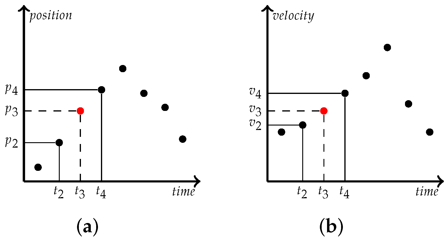
The velocity information of trajectory points is particularly important as a factor of vehicle trajectory data. The velocity information of the vehicle trajectory point can reflect the form of the vehicle at the moment. For example, the higher the velocity value, the better the road network traffic condition, and the lower the velocity value, the worse the road network traffic condition. However, there is another potential knowledge of velocity information that can be mined that is vehicle position. Therefore, this section will describe the relationship between vehicle trajectory point velocity information and position information and road network status information.

From Figure 2a, we can see several continuous trajectory points, and the position information of trajectory points can be deduced according to the time information, which is the traditional vehicle trajectory mining knowledge. In Figure 2b that the relationship between the velocity information of the trajectory point and time can be obtained. Due to the frequency of trajectory acquisition, trajectory points present discrete point states. We can find the acceleration $a(p_i,p_j)$ between any two points in the trajectory at any time from Equation (1).

$$a(p_i,p_j)=\frac{v_j-v_i}{t_j-t_i}$$

(1)

where $v_i$ is initial velocity, $v_j$ is terminal velocity, $t_j-t_i$ is represent use time. The driving state of the vehicle can be obtained by the acceleration change between each trajectory point. The distance formula between two points in the road network is Equation (2).

$$d(p_i,p_j)=║(x_{i+1}-x_i)+(y_{i+1}-y_i)║$$

(2)

where x and y represent the map coordinates of two adjacent trajectory points in the road network respectively, $d(p_i,p_j)$ is $Manhattan$ distance between adjacent trajectory points (Manhattan distance is used because it avoids two adjacent points in a continuous trajectory from appearing in two roads). The relationship between position information and velocity information of trajectory points is expressed by Equation (3).

$$\left\{\begin{array}{cc}\hfill d(p_i,p^{\prime })& =\frac{v^{\prime }+v_i}{2}\times (t^{\prime }-t_i)\hfill \\ \hfill d(p^{\prime },p_j)& =\frac{v_j+v^{\prime }}{2}\times (t_j-t^{\prime })\hfill \end{array}\right.$$

(3)

where $(v^{\prime }+v_i)$ is velocity difference between trajectory points, $(t^{\prime }-t_i)$ is time difference between trajectory points. The mathematical relationships between the $position$, $velocity$ and $time$ of trajectory points are established by Equations (1)–(3).

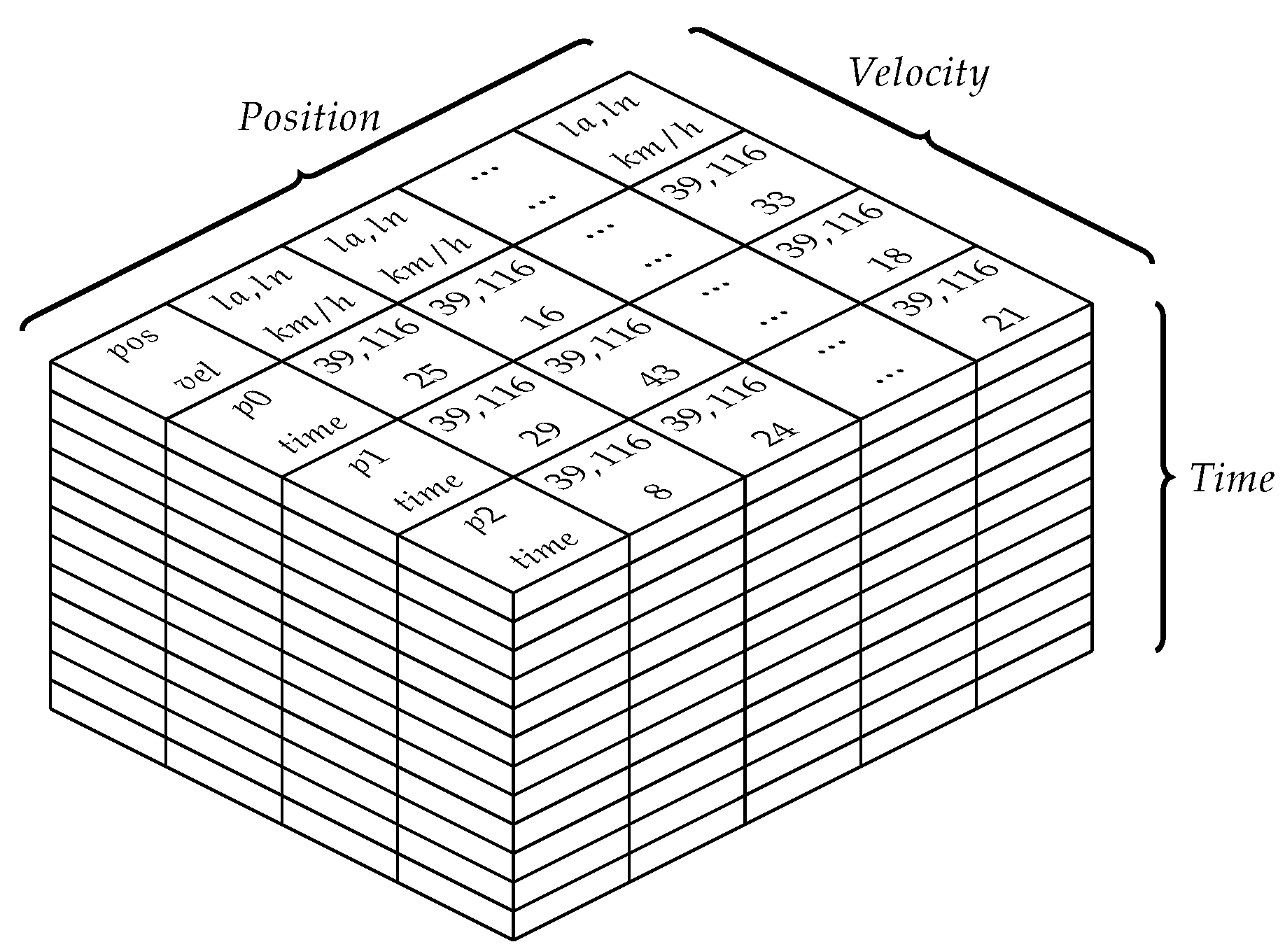
3.2. Trajectory Data Cube Model

This section describes trajectory data cube model to store the position, velocity and time of trajectory points. The purpose is to better represent the temporal and spatial characteristics of trajectory data. The velocity representation of trajectory points is to more accurately restore the position of missing points in the trajectory, which will be introduced in Section 4.

Figure 3 shows the trajectory data cube model, where $pos$ is trajectory point position, $vel$ represents trajectory point velocity, $time$ is trajectory point time-stamp, each row represents a continuous trajectory segment in unit time, each cube piece represents the information of trajectory points. In this paper, trajectory data cube model will be established in unit of minute according to paper [39].

The cube consists of three parts: the position of the trajectory, the velocity, and the time. We design two time unit cubes from the level, so each layer represents the date and hour respectively. Position information of trajectory points in each column of the data cube. We specify that the trajectory points within each road be stored in the same piece (the position points of the road can be determined by two adjacent intersections of the road network dataset), thus, each column represents the same road. Each row is represented as a continuous trajectory in a unit time.

It can be seen from Figure 3 that each time unit is stored in the form of data blocks, and the data time-stamp stored in each layer is the data in the same unit time. The purpose of this design is due to the characteristics of the trajectory data. The amount of trajectory data at each moment is small and sparse. Therefore, if the time-stamp is used as the time unit for storage, a large amount of space will be wasted.

It is worth noting that since latitude and longitude information is not necessarily adjacent to each other in the actual road network when stored (i.e., topology relation is missing), a pointer is added into the small module in each layer named $Topology-Pointer$$\left(TP\right)$, the pointer points to the next position ID adjacent to it. We specify a set $Point$ = {$loc,vel,time,TP$} to represent the points in a trajectory. Therefore, the TDC has the characteristics of vector representation.

It is also worth noting that the selection of unit time requires experimental verification, but we cannot guarantee that vehicles will not run on the same road in unit time. Therefore, this paper has done some processing. Based on our previous research, it is appropriate to change the road network condition in 10–15 min, but data storage at such time interval is still sparse. Therefore, we extend the unit time of the data cube to 30–60 min, so if the same track point appears on the same road in unit time, calculate the average speed of the cube according to Equation (4) and store.

$$vel(v_i,v_j)=\frac{ve{l}_1+ve{l}_2+ve{l}_3+\dots +ve{l}_n}{n}$$

(4)

where $vel(v_i,v_j)$ is the average road network speed expressed between vertices $v_i$ and $v_j$. $ve{l}_1$ is the trajectory point velocity at a certain time. The trajectory point velocities in all time units and on the same road are added and averaged. In this way, all trajectory data is stored in the data cube.

4. Hierarchical Trace-Back Method Based on Trajectory Data Cube

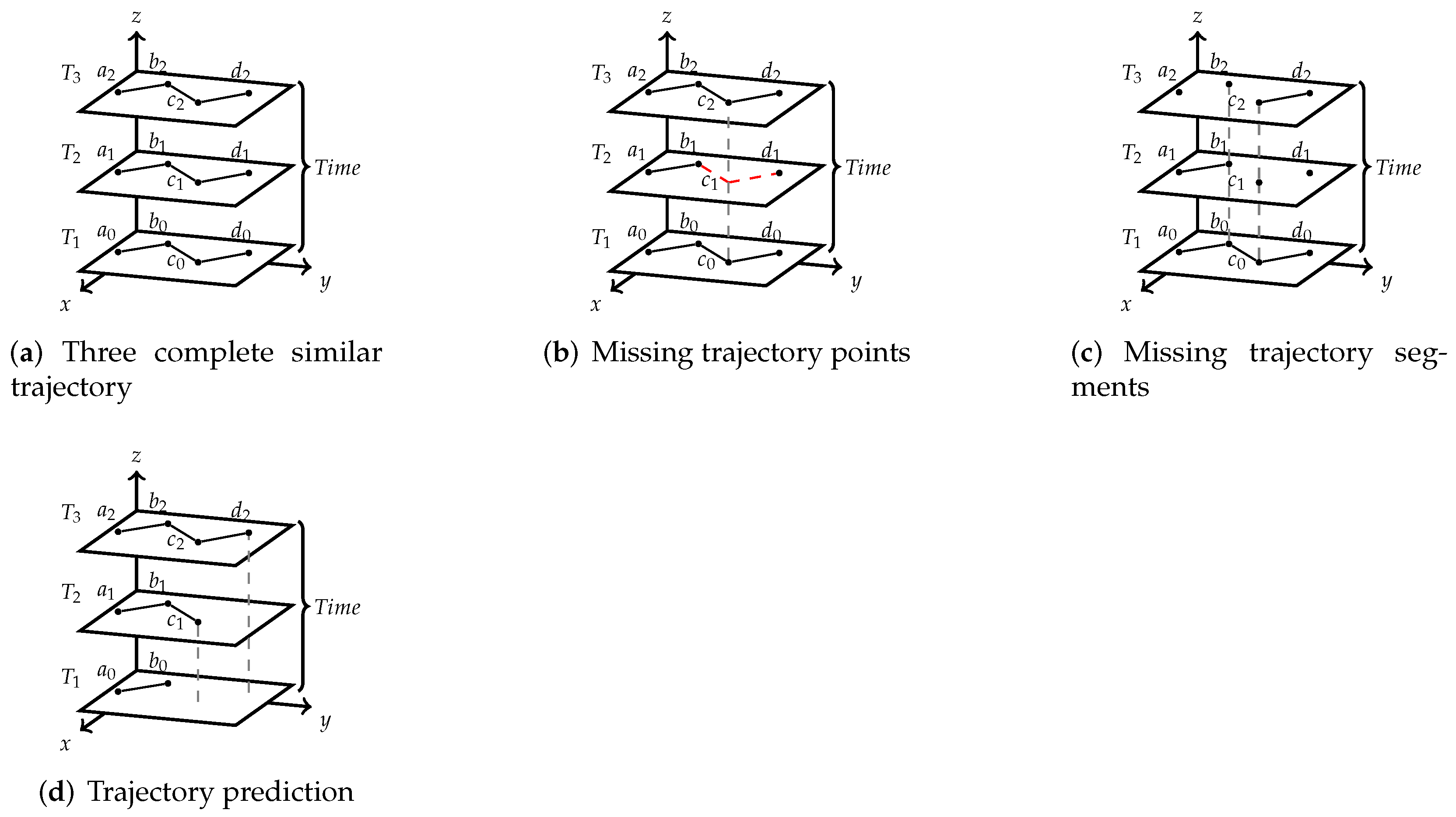
In this section, a hierarchical trace-back (HTB) algorithm based on spatio-temporal trajectory data will be introduced. This method includes a Bayesian probability method, which is used to restore the missing points or missing trajectory segments in the trajectory. The purpose of classifying trajectory data according to time hierarchy is to find out the spatio-temporal features hidden in the trajectory.

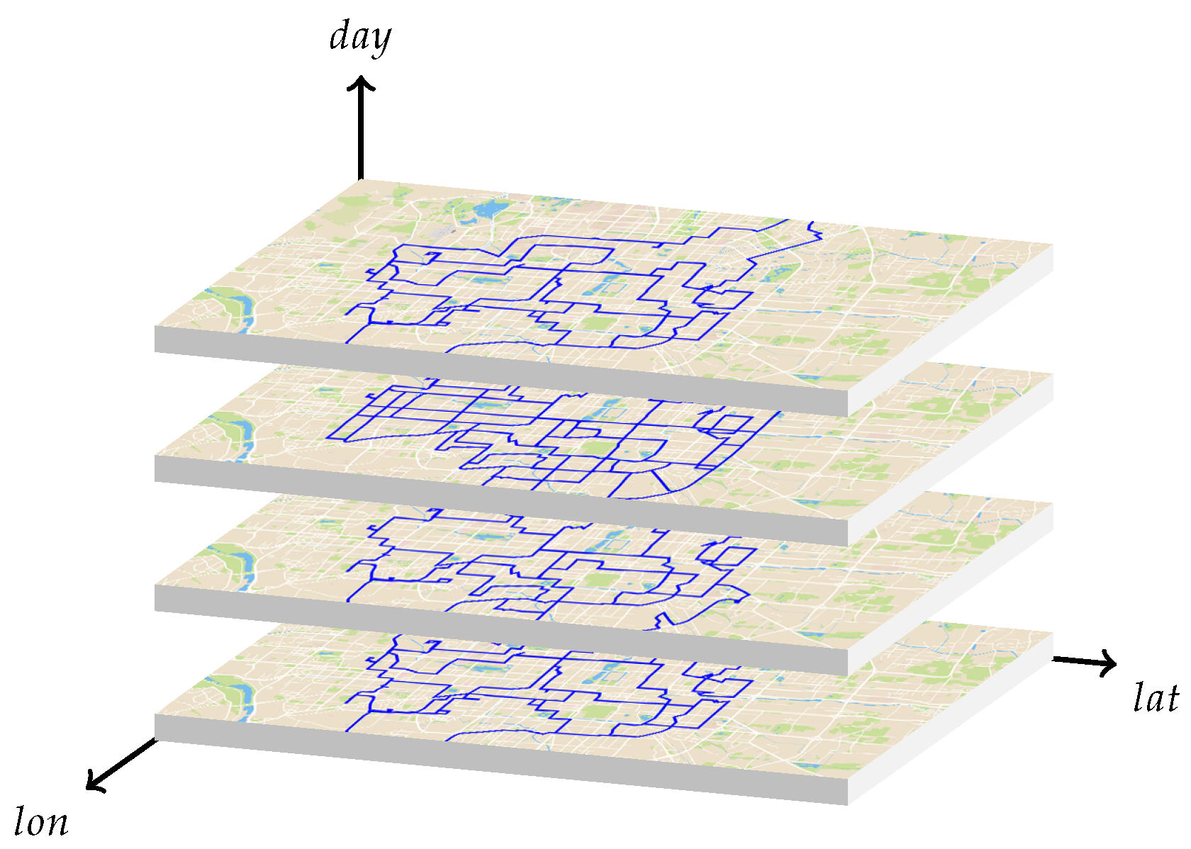
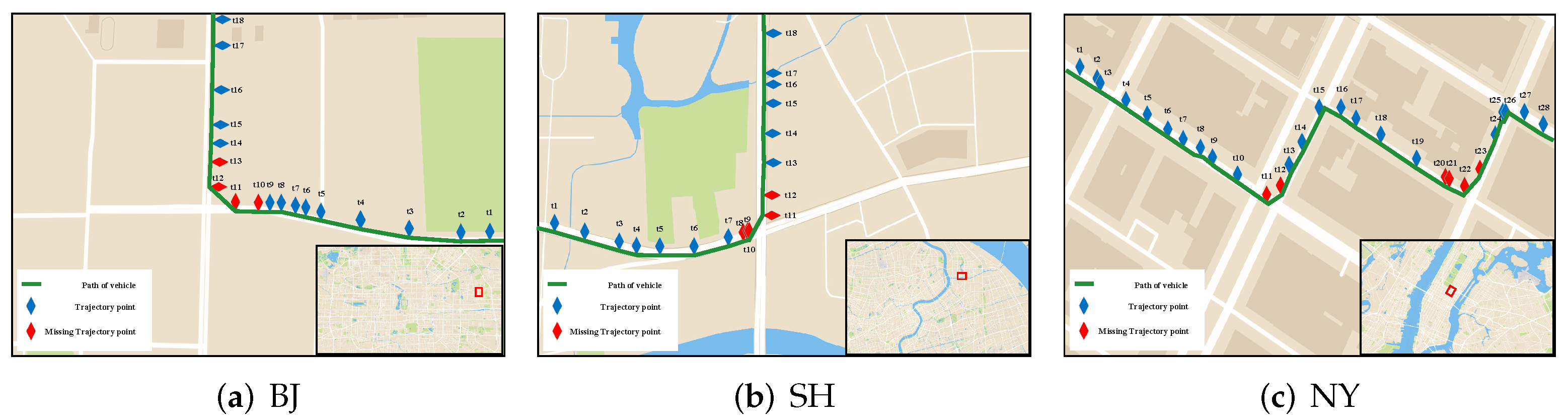
Figure 4 shows the trajectory chart of a vehicle in four days, from which it can be seen that the same path or different paths occurred in four days. The purpose of HTB algorithm is to focus on the similar trajectories that appear in the same time period in different dates, and these trajectories are classified and stored by TDC model. In trajectory data, time information is generally not lost or missing, and what the equipment usually records is the time information when the data is generated (especially the trajectory data collected under the condition of constant frequency). Even in the case of unequal frequency there is still a definite time period. Therefore, the most important information restoration is the position information and velocity information of trajectory points.

4.1. Trajectory Position Restoration Based on TDC Model

In the actual trajectory dataset, there are often trajectory points with inaccurate trajectory positions, which are often caused by unstable equipment signals or vehicles in a space blocked by signals. Therefore, the missing or offset of trajectory position information in this paper can be completed by TDC and hierarchical trace-back position (HTB-p) algorithm. The calculation process of HTB-p will be described the following.

Definition 1.

Given a missing dataset M, according to the trajectory data characteristics, there is a continuous trajectory segment P $<p_i,p_m,p_j>$, where $p_m$ is the missing trajectory point, then the time information of the point can obtain the time range of missing data from the time of $p_i$ and the time of $p_j$.

Definition 1 gives the time range of missing data. Similarly, the position area of the missing trajectory can be determined according to the front and rear position information segments of the missing trajectory data.

Definition 2.

Given a missing dataset M, there is a continuous trajectory segment P $<p_i,p_m,p_j>$, where $p_m$ is the missing trajectory point, then the position information of the point can obtain the position area of missing data from the position of $p_i$ and the position of $p_j$.

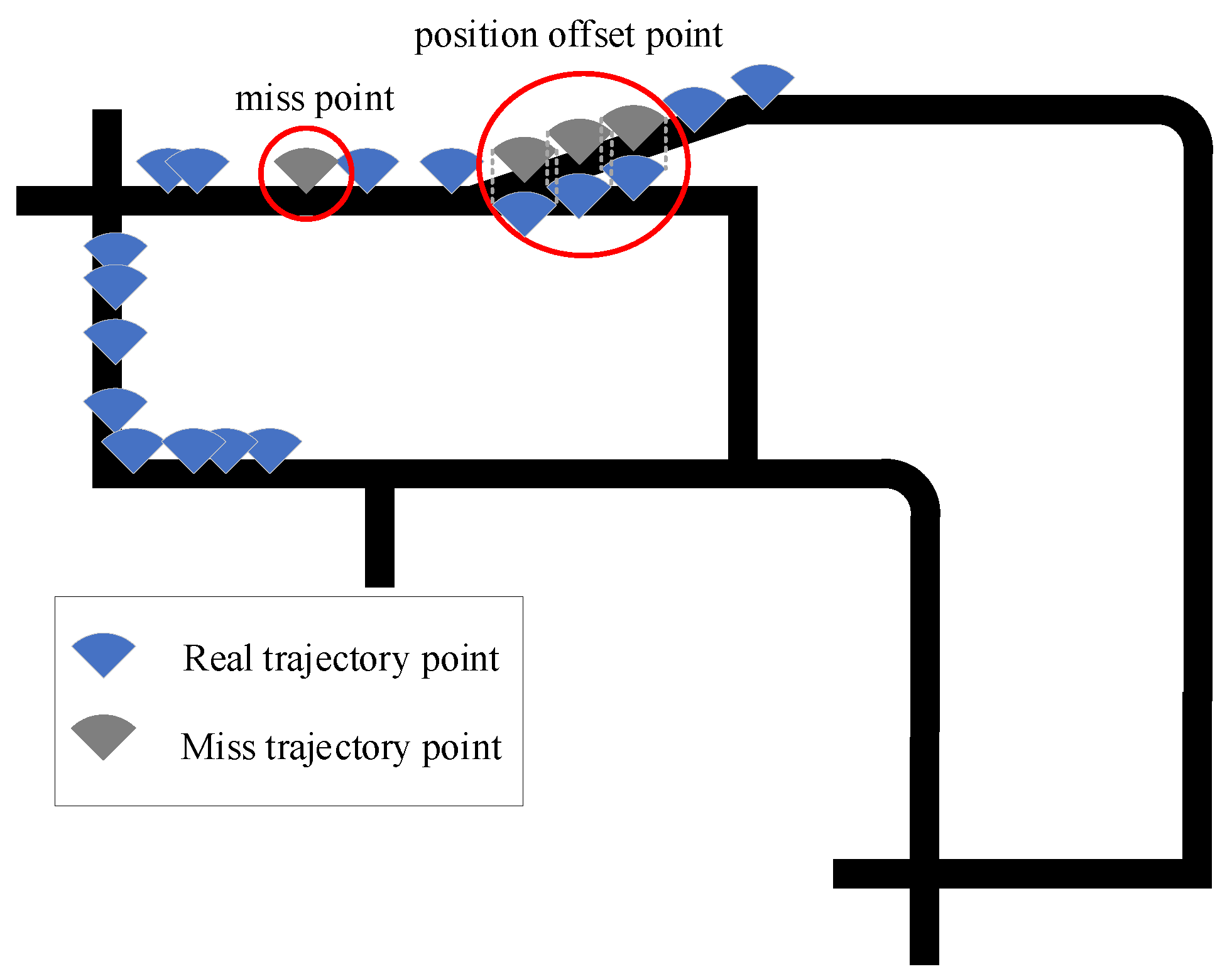
Definition 2 gives the position area of missing data. According to Definition 1, Definition 2 and TDC, the trajectory data information of all lost data in the same time period in history can be obtained. The information related to missing data is extracted hierarchically from TDC. Figure 5 shows the examples of missing position information and position offset of trajectory points.

The core of HTB-p algorithm is the process of calculating the information in the time period extracted by TDC. HTB-p algorithm is divided into two steps; 1. By lack of traversal path set point data, matching with the data in the TDC and search, through the corresponding time to get the corresponding TDC layer, and return loss trajectory points corresponding to the data information in the TDC, with this information as the keyword as a search condition, then return all trajectory data information of different levels in the same time. 2. All the qualified information obtained from TDC is calculated for conditional probability. According to the condition of time and velocity, the probability statistics of all possible road ID are carried out. Finally, the road ID with higher probability is returned to the missing trajectory data, and the position is marked as the position information of the missing trajectory point. Algorithm 1 introduces a HTB-p method with position information of the missing trajectory point.

Algorithm 1 HTB-p

1: Input: TDC, M 2: Output:$Tra<P,V,T>$ 3: Initialization$Tra<P,V,T>$, MapSet $prob$ 4: forMdo 5:    search $M_p\left(time\right)$ from TDC 6:    compare $Time$ in each level 7:    if $Time$$==$$M\left(time\right)$ then 8:        Calculation $Pr\left(p_i\right|v,t)$ = $\frac{Pr\left(p_i\right)Pr\left(v\right|p_i)Pr\left(t\right|p_i,v)}{Pr\left(v\right)Pr\left(t\right|v)}$ 9:        $prob$.put($p_i$,$Pr\left(p_i\right|v,t)$) 10:    end if 11:    get $p_i$ with maximum $Pr$ value from $prob$ 12:    $Tra<P,V,T>$ = $p_i$ 13:    TDC = $Tra<P,V,T>$ 14: end for 15: RETURN TDC

Where M is missing trajectory set, $Tra<P,V,T>$ is contain the position, velocity, and time with one point in the trajectory. $M_p\left(time\right)$ is time of loss trajectory point, $Pr$ represents the probability of candidate position. $prob$ stores the probability of each candidate position. $M\left(time\right)$ is the time of missing trajectory point, $p_i$ is miss point ID. Lines 4–6 describe obtaining the ID of trajectory points from the missing trajectory set M in turn, and obtaining all trajectory information in the same time layer in TDC by comparing with the time in TDC. Lines 7–9 find the trajectory data block with the same time as that in the M set from the TDC, return all the trajectory information in the block, calculate all candidate points in the TDC through Bayesian conditional probability. Line 11–15 finally return the value with the maximum probability, and supplement the information of the missing points to the TDC. Since there is only one loop in the algorithm, the time complexity of the algorithm is $O\left(n\right)$, where n is the number of missing trajectory points.

4.2. Trajectory Velocity Restoration Based on TDC Model

A HTB-v method will be introduced in this section, which aims to supplement the trajectory points without measured velocity information in the trajectory. Since the known information includes position information and time information, the missing velocity information is calculated according to the structural characteristics of the TDC. Firstly, the position points with missing velocity information can be obtained according to the position information. In this process, the position of the missing velocity trajectory point set can be classified through the position classification module of the TDC to screen the accurate position. Secondly, the time of the missing trajectory point set is matched with the time layer divided by the data cube, and the missing trajectory point set is divided into the corresponding time layer. Through the above two steps, all points in the trajectory point set with missing velocity information are divided into TDC blocks.

Definition 3.

Given a missing velocity dataset M, according to the trajectory data characteristics, there is a continuous trajectory segment P $<p_i,p_m,p_j>$, where $p_m$ is the missing velocity trajectory point, then the position information of the point can obtain from the $p_i$$\left(position\right)$ and $p_j$$\left(position\right)$, the time information of the point can obtain the time range of missing data from the $p_i$$\left(time\right)$ and $p_j$$\left(time\right)$.

Definition 3 gives the position information and the time range of missing data. the following we need to calculate the missing velocity information in the trajectory point. We still need to calculate the probability of the trajectory block in the TDC with the help of Bayesian conditional probability formula, and finally return the maximum speed probability value, and the result is returned to the specific missing point. Algorithm 2 describes the process of restoring trajectory points with missing velocity information by HTB algorithm.

Algorithm 2 HTB-v

1: Input: TDC, M 2: Output:$Tra<P,V,T>$ 3: Initialization$Tra<P,V,T>$, MapSet $prob$ 4: forMdo 5:     search $M_v\left(position\right)$ from TDC 6:     compare $position$ in TDC 7:     if $position$$==$$M_v\left(position\right)$ then 8:        search $M_v\left(time\right)$ from TDC 9:        compare $Time$ in each level 10:       if $Time$$==$$M\left(time\right)$ then 11:          Calculation $Pr\left(p_i\right|p,t)$ = $\frac{Pr\left(p_i\right)Pr\left(v\right|p_i)Pr\left(t\right|p_i,p)}{Pr\left(v\right)Pr\left(t\right|v)}$ 12:          $prob$.put($p_i$,$Pr\left(p_i\right|p,t)$) 13:       end if 14:    end if 15:    get $p_i$ with maximum $Pr$ value from $prob$ 16:    $Tra<P,V,T>$ = $p_i$ 17:    TDC = $Tra<P,V,T>$ 18: end for 19: RETURN TDC

Where M is missing trajectory set, $Tra<P,V,T>$ is contain the position, velocity, and time with one point in the trajectory. $M_v\left(position\right)$ is position of loss trajectory point, $M_v\left(time\right)$ is time of loss trajectory point, $Pr$ represents the probability of candidate position. $prob$ stores the probability of each candidate position. $M\left(time\right)$ is the time of missing trajectory point, $p_i$ is miss point ID. Lines 4–9 describe obtaining the ID of trajectory points from the missing trajectory set M in turn, and obtaining all trajectory information in the same time layer in TDC by comparing with the time in TDC. Lines 10–12 find the trajectory data block with the same time as that in the M set from the TDC, return all the trajectory information in the block, calculate all candidate points in the TDC through Bayesian conditional probability. Line 15–19 finally return the value with the maximum probability, and supplement the information of the missing points to the TDC. Since there is only one loop in the algorithm, the time complexity of the algorithm is $O\left(n\right)$, where n is the number of missing trajectory points.

4.3. Trajectory Position and Velocity Restoration Based on TDC Model

The road network state restoration method when there are continuous and missing position information and trajectory velocity in the trajectory segment will be introduced in this section. Kalman-Filtering (KF) [40] and variants can effectively restore the missing trajectory, but the restoration strategy for multi vehicle trajectory loss in the road section and road network traffic flow still needs to be improved. Therefore, this section will introduce a hierarchical backtracking algorithm HTB-KF that combines KF and TDC.

Firstly, the missing position information in the trajectory data is restored for the first time by KF algorithm. The restored information is returned to the missing trajectory set and TDC. The position information in TDC and the missing trajectory is compared, and the position information and time information are matched once. Secondly, the velocity information of missing trajectory points is assigned. The result of matching the position information restored by KF with TDC is returned to the missing trajectory point, the matching velocity information value is found from the TDC block, the probability superposition is carried out through the position front-rear information and time information, and finally the velocity information with the greatest probability is returned to the missing trajectory point. Equations (5) and (6) describe the trajectory data process of KF. It is worth noting that this paper compares the position information and velocity information of lost trajectory points as restored separately, so only a single element of information restore is considered when using KF method. A trace-back mechanism will be added in this section to verify the missing information.

$$x_k=A{x}_{k-1}+B{u}_{k-1}+w_{k-1}$$

(5)

where A is the state transition matrix and w is the process noise. The state transition matrix A is determined according to the kinematic formula, B is the matrix that takes part of influencing the system state change.

$$z_k=H{x}_k+e_k$$

(6)

where z represents the predicted value, and H is the conversion matrix from the current measured value to the predicted measured value. e represents noise. In this paper, the position of the missing trajectory is predicted for the first time with the assistance of KF [40]. The velocity information of the missing trajectory data is assigned by the restored position information and TDC. The position information is checked by TDC again after the assignment. Algorithm 3 describes the calculation process of HTB-KF.

Where M is missing trajectory set, $Tra<P,V,T>$ is contain the position, velocity, and time with one point in the trajectory. Lines 4–6 describe the preliminary judgment of the missing trajectory position using KF. Lines 7–17 calculate the position information obtained through KF, so as to deduce the velocity information of missing trajectory points. Line 18 is to recheck the position obtained by KF, so as to further reduce the error. Lines 19–23 return the final result and store it in TDC. The time complexity of the HTB-KF algorithm is $O\left(n^2\right)$, where n is the number of missing trajectory points.

Algorithm 3 HTB-KF

1: Input: TDC, M 2: Output:$Tra<P,V,T>$ 3: Initialization$Tra<P,V,T>$, MapSet $prob$ 4: forMdo 5:    Calculation of M by KF 6: end for 7: forM with position information do 8:     search $M_v\left(poistion\right)$ from TDC 9:     compare $position$ in TDC 10:    if $poistion$$==$$M\left(position\right)$ then 11:       search $M_v\left(time\right)$ from TDC 12:       compare $Time$ in each level 13:       if $Time$$==$$M\left(time\right)$ then 14:          Calculation $Pr\left(p_i\right|p,t)$ = $\frac{Pr\left(p_i\right)Pr\left(v\right|p_i)Pr\left(t\right|p_i,p)}{Pr\left(v\right)Pr\left(t\right|v)}$ 15:          $prob$.put($p_i$,$Pr\left(p_i\right|p,t)$) 16:       end if 17:    end if 18:    HTB-p 19:    get $p_i$ with maximum $Pr$ value from $prob$ 20:    $Tra<P,V,T>$ = $p_i$ 21:    TDC = $Tra<P,V,T>$ 22: end for 23: RETURN TDC

5. Experimental

In this section, the experimental process and parameter settings will be introduced in detail. In this paper, three types experiments will be conducted. The first experiment is to validate the proposed HTB-p algorithm for restoration of missing position information points in trajectory dataset. The second experiment is to verify HTB-v algorithm for restoration of missing velocity information points in trajectory dataset. The third experiment is to verify HTB-KF algorithm for restoration of missing position and velocity information points in trajectory dataset.

5.1. Experiment Setting

All experiments are implemented in Java, Python, and all algorithms are executed on 16G memory, 64-bit Windows 10 operating system, and Intel i5 @3.30 GHz CPU. The road network data in this paper comes from the Beijing map data, Shanghai map data, and New York map data of OpenStreetMap (https://www.openstreetmap.org) (accessed on 5 December 2020) The vehicle trajectory data is three months and the size is 57 G with Beijing Taxi in 2012.4 and 2013.6–2013.7 (Beijing Municipal Commission of Communications), one day and size is 332 MB with Shanghai Taxi in 2007 (https://cse.hkust.edu.hk/scrg/, accessed on 1 February 2022), and size is 119 GB New York Yellow Taxi Trip Records in 2019 (https://www1.nyc.gov/site/tlc/about/tlc-trip-record-data.page, accessed on 1 February 2022).

Table 2. Datasets.

$\mathbf{Dataset}$	$\mathbf{Region}$	$\mathbf{Size}$
BJ	Beijing	57 G
SH	Shanghai	332 MB
NY	New York	119 GB

shows the information of the dataset. Visualization using Mapbox API (https://studio.mapbox.com/, accessed on 1 February 2022). Since the vehicle dataset in New York only has position information and does not have velocity information, the verification based on velocity information restoration will not be used. However, the average speed of the vehicle can still be obtained after the processing of position information and time information, so it can be used for the verification of the Section 5.4.

5.2. Verification of Missing Trajectory Position Based on TDC Hierarchical Trace-Back Method

Firstly, the trajectory details of the three main roads in the three sample datasets are extracted, as shown in Figure 6.

The gray icons in Figure 6 is the trajectory position information points $\Psi$ {$p_n$} deleted from the original trajectory set, but these points retain time information and velocity information. The following will compare the position restoration results of the proposed HTB-p algorithm and the existing trajectory position completion algorithm. Figure 7 shows the experimental comparison of HTB-p based on TDC with other trajectory position restoration algorithms.

From Figure 7 show the effective of KF algorithm, Interpolation algorithm and HTB-p algorithm on restoring the trajectory, and compare it with the actual GPS trajectory. Figure 7a shows the restoration of a continuous trajectory based on taxis in Beijing. According to the four position of the missing trajectory selected in Figure 6a, it can be seen that the position information restored by HTB-p is better than that of KF and Interpolation algorithm. Figure 7b shows the restoration of a continuous trajectory based on taxis in Shanghai. According to the five position of the missing trajectory selected in Figure 6b. Figure 7c shows the restoration of a continuous trajectory based on taxis in New York. According to the six position of the missing trajectory selected in Figure 6c.

The effect of interpolation algorithm is better because there are points with continuous missing position information, so multiple interpolation operations are required, which has poor effect. Although the effect of KF is better than the interpolation algorithm, its calculation core is to predict the results of this time based on the results of the previous calculation. Therefore, when there are missing continuous trajectory points, the restoration effect of KF algorithm depends on the results of the previous calculation. HTB-p not only calculates the missing trajectory position points according to the front-rear point information of the trajectory, but also needs to evaluate and compare the probability of historical position through the condition of historical data. Therefore, HTB-p has good calculation results.

Table 3. The result of Mean Euclidean Error [m] between predicted value and actual value.

		Datasets	BJ	SH	NY
	MEE
Methods
KF			26.470	42.614	14.155
Interpolation			27.529	45.847	16.238
HTB-p			11.982	19.347	8.786

shows the Mean Euclidean Error (MEE) between the position obtained by the three algorithms and the actual position, dimension is [m], the average of all error distances is shown Table 3.

$$MEE=\frac{{\sum }_{i=1}^n\sqrt{{(x_f-x_m)}^2+{(y_f-y_m)}^2}}{n}$$

(7)

Equation (7) describes the calculation process of MEE. Where n is the number of missing trajectory points, ($x_f$, $y_f$) is estimated position point, ($x_m$, $x_m$) is position of actual missing trajectory points.

Table 3 can see the average error between the predicted value and the actual value of the three algorithms. The error distance of the interpolation algorithm is much greater than that of KF algorithm and HTB-p algorithm. There is a certain relationship between the effect of the trajectory completion algorithm and the dataset itself. It can be seen from Table 3 that the trajectory error of taxis based on the average error is related to the distance and time according to the trajectory information before and after the missing trajectory points. When the trajectory information front-rear missing trajectory points is known, the effect of interpolation trajectory is better. When the front-rear trajectory information positions of trajectory points are missing, the restoration effect of HTB-p is better.

5.3. Verification of Missing Trajectory Velocity Based on TDC Hierarchical Trace-Back Method

This section will continue to select three consecutive tracks from three trajectory samples for verification. According to Figure 6, the velocity information of the missing points in the figure is deleted, and the position information is added to the dataset. The experiments in this section will verify the velocity information $\Psi${$v_n$} restoration and sample error rate of the three algorithms for missing trajectory points in three datasets.

Figure 8 show the restoration of position information by KF algorithm, Interpolation algorithm and HTB-v algorithm, and Figure 8a shows the velocity restoration based on Beijing vehicle trajectory. It can be seen from the figure that when the velocity information of continuous trajectory points is missing, the effect of KF is better than Interpolation, and the effect of HTB-v is similar to that of KF. Similarly, it can be seen from Figure 8b that the effect of Interpolation algorithm is worse, while the effect of KF and HTB-v algorithm is better.

Table 4. The error rate $\varphi$ of the three algorithms.

Methods	BJ				SH
	$t10$	$t11$	$t12$	$t13$	$t8$	$t9$	$t10$	$t11$	$t12$
KF	11.0%	9.0%	7.5%	8.2%	6.7%	23.0%	33.5%	5.0%	2.9%
Interpolation	21.0%	20.6%	21.3%	8.0%	13.3%	21.0%	70.0%	24.0%	6.4%
HTB-v	6.4%	8.9%	4.3%	6.5%	1.7%	12.4%	30.0%	2.1%	1.4%

shows the error rate $\varphi$ of the algorithm to restore the trajectory velocity.

$$\varphi =\frac{|ve{l}_f-ve{l}_a|}{ve{l}_a}\times 100\%$$

(8)

Equation (8) describes the calculation process of $\varphi$. Where $ve{l}_f$ is estimated velocity value, $ve{l}_a$ is velocity value of actual trajectory data.

It can be seen from Table 4 that the three algorithms restore the velocity of two datasets. The error rate of Interpolation algorithm is significantly higher than that of other algorithms (The percentage data of reaction in the table refers to the error rate between the actual velocity value and the restored velocity value), For example, at t12, the error rate of Interpolation is 20.6%, while the error rates of KF and HTB-v are 9.2% and 8.9% respectively. The reason is that when there are continuous missing trajectory points, the Interpolation algorithm can not effectively process the data (the Interpolation algorithm depends on the trajectory information before and after the missing trajectory points). The restoration of KF and HTB-v algorithms is better, but the $\varphi$ value is still large. The main reason is because of the training sample set. The Section 5.4 will train and model all trajectory datasets.

5.4. Verification of Missing Trajectory Position and Velocity Based on TDC Hierarchical Trace-Back Method

This section will complete and verify the data of multiple trajectory segments in the trajectory by training all trajectory set samples. In this section, 70% of the three datasets are used as training sets and 30% as restore test sets for verification. A group of experiments delete the position information and velocity information of the remaining 5%, 10%, 15%, 20%, 25%, and 30% of the dataset through the training and backtracking dataset, retain the time data, and restore it. The other group is to change the number of training sample sets to restore the trajectory information in the remaining datasets.

Firstly, HTB-KF is compared with the existing trajectory completion algorithm. From Figure 9 shows that the restoration of three trajectory datasets by different algorithms, and the effect of algorithm restoration through MEE.

The experiment compares KF, LSTM, MDCGCN, Interpolation and HTB-KF algorithms to restore the trajectory by training the data of three trajectory sets. It can be seen from Figure 9a that with the increase of the number of restored trajectory datasets, HTB-KF and MDCGCN algorithms have better restoration effects. The reason why interpolation algorithm restores trajectory query is that it needs to rely on the information of adjacent trajectory points of missing trajectory points for interpolation. However, when there are segments of missing trajectory in the dataset, the restoration effect is poor. It is not suitable for restoring a large number of trajectory segments. The restoration effect of KF and LSTM algorithms is slightly worse than that of MDCGCN and HTB-KF.

Figure 9b shows the restoration of Shanghai vehicle trajectory dataset by the algorithm. The same HTB-KF and MDCGCN have better effects. Figure 9c shows the restoration of New York vehicle trajectory datasets by the algorithm. However, the effect of Figure 9b is worse than that of Figure 9c. The reason is that the trajectory datasets in Shanghai has only one day, and its sample size is smaller than that of Beijing and New York. Therefore, the overall restoration effect is worse than that of the other two sample sets. However, even if the sample size of the dataset is insufficient, HTB-KF algorithm still has satisfactory restoration effect.

Figure 10 represent the restoration of velocity information in the trajectory segments of two datasets by different algorithms. Figure 10a restores the information in the trajectory set in Beijing. It can be seen from the figure that with the increase of the number of restored samples, the error rate of KF, LSTM, MDCGCN and HTB-KF algorithms is also increasing, but the growth slope is lower than that of other algorithms.

Figure 10b restores the velocity information in the trajectory set of Shanghai. From the figure can be seen that the error rate of the algorithm is also increasing with the increase of the number of samples. Compared with Figure 10a, the error rate $\varphi$ is higher because the number of training samples in Shanghai is small, so the information error rate restored by the algorithm is higher. The error rate $\varphi$ of Interpolation algorithm is higher than that of other algorithms. The main reason is that the essence of its restoration theory requires the lack of trajectory information front-rear trajectory information.

The following experiment verifies that the HTB-KF algorithm restores vehicle velocity based on the Beijing trajectory datasets and Shanghai trajectory datasets. This experiment sets up an intersection on each trajectory set to be the most observable intersection. Figure 11 show the BJ datesets chooses the intersection of Dongsanhuan Road and Guangqu Road (116°46′80.48″ E, 39°89′91.33″ N), and SH datesets chooses the intersection of Jiujiang Road and Henan Middle Road (121°49′17.69″ E, 31°24′24.17″ N).

Figure 11a shows a curve comparison of the true data and the completion value at 9:00–11:00 on a certain day in the Beijing datasets with a data loss rate of 20% (time interval 5 min), Figure 11b shows a curve comparison of the true data and the completion value at 18:00–20:00 on a certain day in the Shanghai datasets with a data loss rate of 20% (time interval 5 min). From the graph, it can be seen that the completion result of the HTB-KF method is very close to the true situation of the ground, and can capture the dynamic changes of traffic velocity in the complex conditions of early and late rush hours. The results of the completion fluctuate very smoothly compared with the ground truth. In summary, the HTB-KF methods presented in this paper can interpolate the traffic situation reasonably.

6. Conclusions

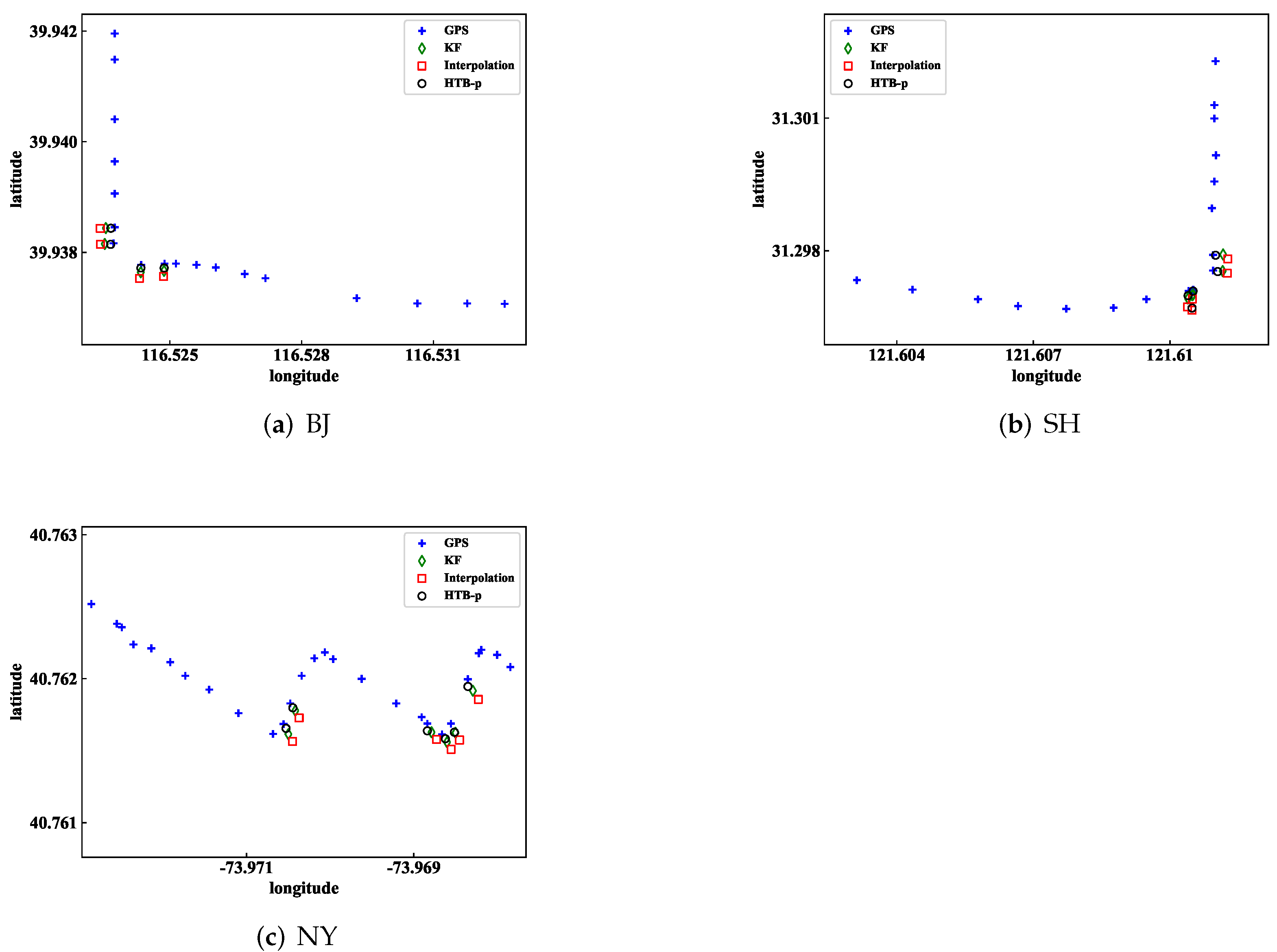
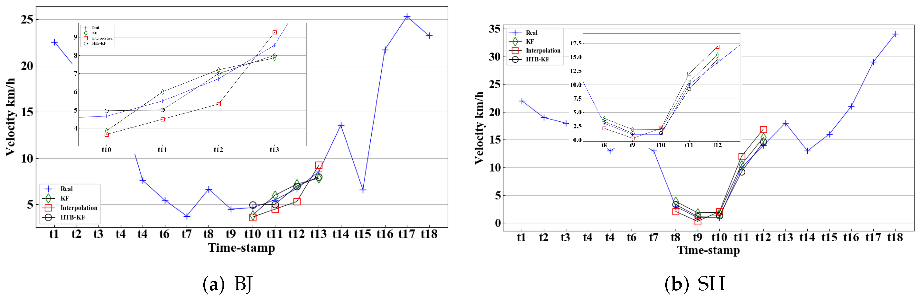
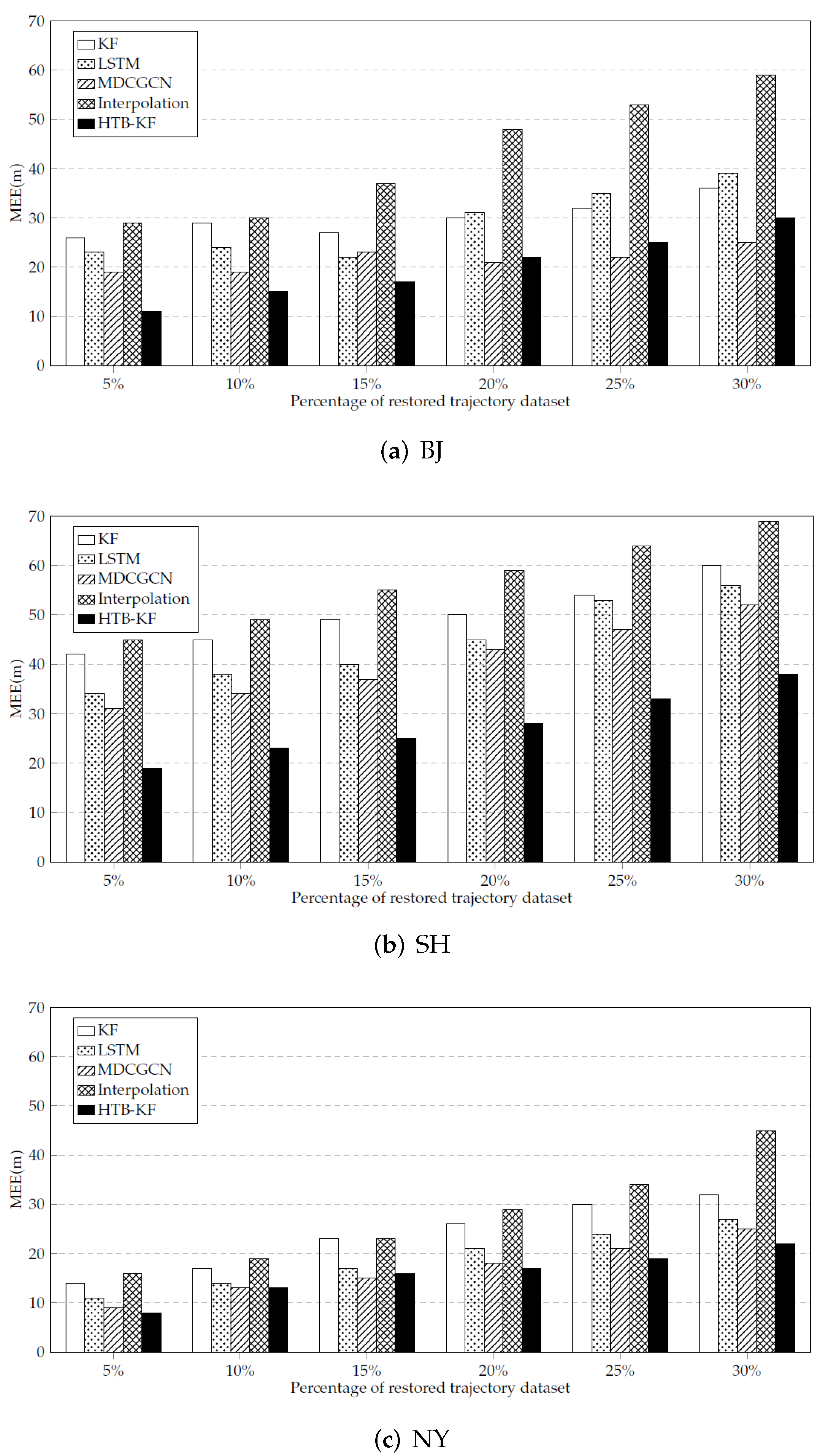
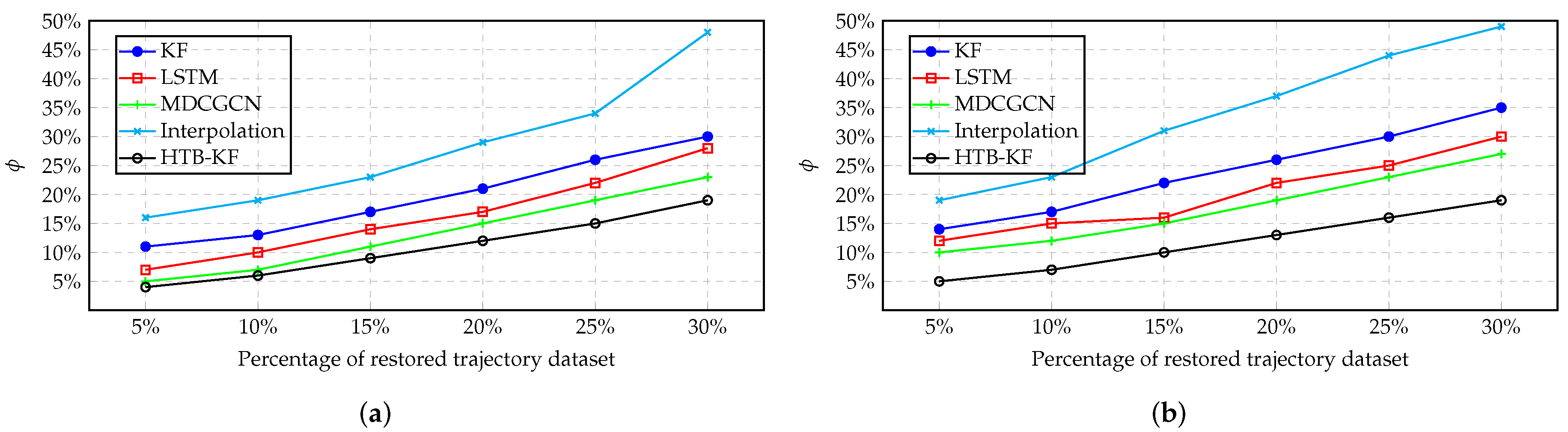
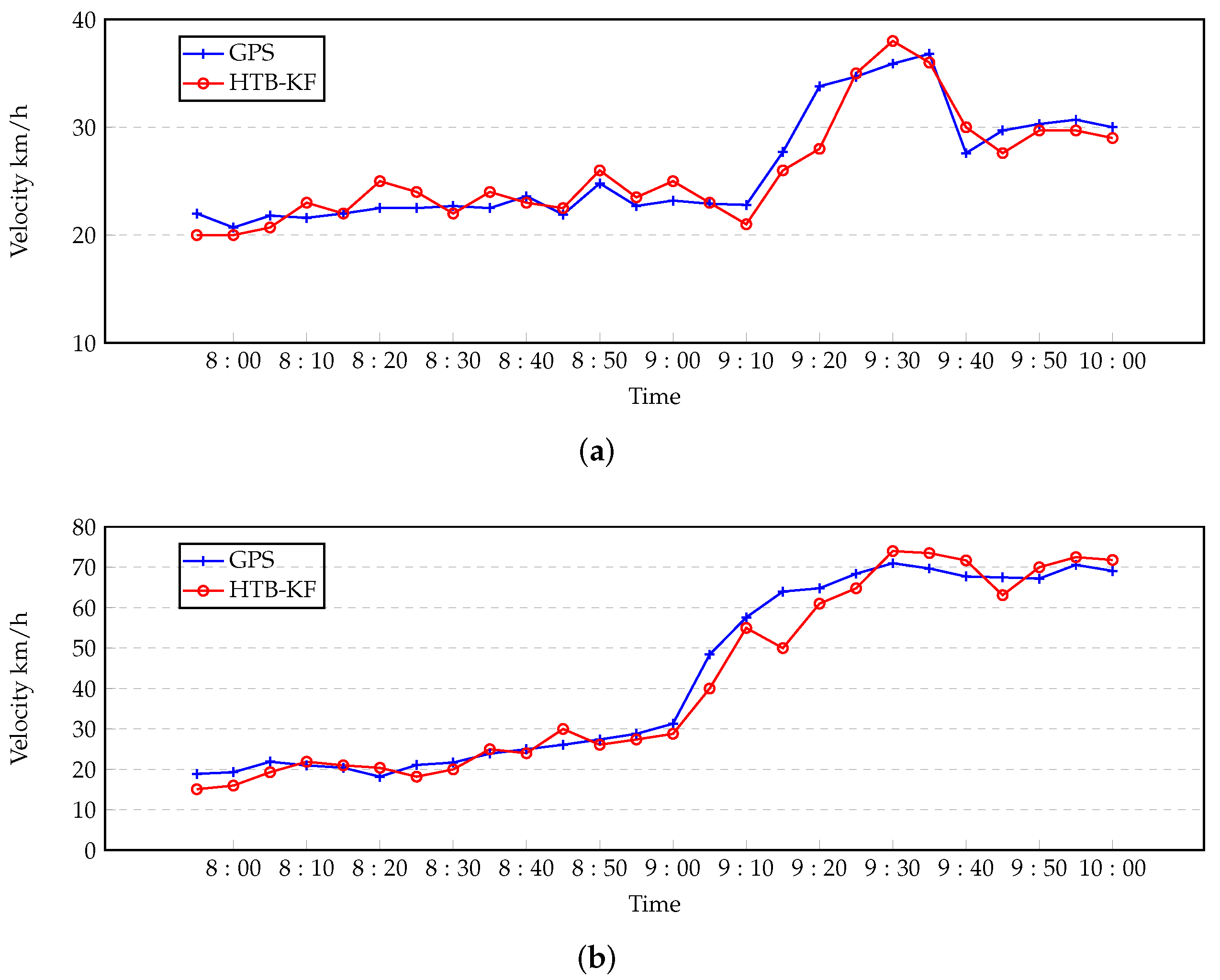
In conclusion, a novel trajectory data cube (TDC) is introduced to model, analyze and process trajectory data in this paper. Three trajectory hierarchical trace-back algorithms based on the TDC model are designed to restore the missing information in the trajectory, and to restore the traffic flow of the missing trajectory. Because the position information and velocity information in the trajectory information can effectively explain the traffic manifold at that time. Finally, in the experimental part, the trajectory restoration of the HTB-p, HTB-v, and HTB-KF algorithms is verified. Firstly, the HTB-p method is verified the restoration of the missing position of individual trajectory points in the trajectory segment by HTB-p method (there are few training sample sets in this experiment, and all trajectory sets are not processed), and its MEE and error rate are less than those of other methods. Secondly, the HTB-v method is verified to restore the velocity information of individual trajectory points in the trajectory segment. Through experimental comparison, it can be concluded that the HTB-v method has a better restoration effect. Thirdly, the restoration of missing trajectory segment information by HTB-KF algorithm is verified. It is also verified that HTB-KF algorithm can restore driving conditions, and it is found that HTB-KF algorithm still has good restoration ability when the sample training set is limited.

In future work that we will add the deviation angle of trajectory information as a factor of trajectory information, and try to complete the missing part of trajectory datasets with less training sample size.