VINS-Dimc: A Visual-Inertial Navigation System for Dynamic Environment Integrating Multiple Constraints

Abstract

Most visual–inertial navigation systems (VINSs) suffer from moving objects and achieve poor positioning accuracy in dynamic environments. Therefore, to improve the positioning accuracy of VINS in dynamic environments, a monocular visual–inertial navigation system, VINS-dimc, is proposed. This system integrates various constraints on the elimination of dynamic feature points, which helps to improve the positioning accuracy of VINSs in dynamic environments. First, the motion model, computed from the inertial measurement unit (IMU) data, is subjected to epipolar constraint and flow vector bound (FVB) constraint to eliminate feature matching that deviates significantly from the motion model. This algorithm then combines multiple feature point matching constraints that avoid the lack of single constraints and make the system more robust and universal. Finally, VINS-dimc was proposed, which can adapt to a dynamic environment. Experiments show that the proposed algorithm could accurately eliminate the dynamic feature points on moving objects while preserving the static feature points. It is a great help for the positioning accuracy and robustness of VINSs, whether they are from self-collected data or public datasets.

1. Introduction

Visual simultaneous localization and mapping (SLAM), which uses image data from cameras, is one of the most important topics in computer vision [1,2]. This technology has important applications in robotics [3,4], autopiloting [5,6], and augmented reality [7,8].

When SLAM technology integrates an inertial measurement unit (IMU) and cameras, it is called a visual–inertial navigation system (VINS). The best known VINS is VINS-mono [9], which was proposed by Qin et al. This system achieves accurate positioning of a device by observing visual feature points and pre-integrated IMU measurements. It can also compute and calibrate extrinsic and temporal offsets between the camera and IMU online. OKVIS [10] uses the concept of “keyframes” that partially marginalize old states to keep computational costs low, and ensure real-time operation. ROVIO [11] directly uses the pixel intensity errors of the images, and it can achieve accurate tracking performance with great robustness. A novel VINS based on an extended Kalman filter was proposed, named MSCKF [12]. The measurement model can express the geometric constraints, which is useful for system localization. An open platform named OpenVINS was proposed by Geneva et al. [13]. It uses some technologies, such as a sliding window Kalman filter, consistent First-Estimates Jacobian treatments and SLAM landmarks.

However, most VINSs are focused static environments [14]. In a front-end visual odometer module, the system extracts the feature points on visual images. Then, the system matches the feature points of two adjacent frames. Then, the position and attitude of the camera and the position of the feature points in the real world are determined by a local bundle adjustment of the visual and IMU data in the sliding window. The residual of the bundle adjustment optimization which should be minimized can be formulated as follows [15]:

$$R={\sum }_{k=1}^m {\sum }_{i=1}^n w_{k,i}{\left(u_{k,i}-\pi \left({\mathit{T}}_k,{\mathit{p}}_i\right)\right)}^2+r_B,$$

(1)

where R is the sum of the residuals, m is the number of images, and n is the number of feature points. If the 3D key point ${\mathit{p}}_i$ can be observed in the image k, the value of $w_{k,i}$ is set to 1; otherwise, it is set to 0. Here, $u_{k,i}$ represents the two-dimensional (2D) coordinates in image k of 3D point ${\mathit{p}}_i$. Moreover, π represents the projection of a 3D key point onto an image based on the position, pose, and intrinsic parameters of the cameras. Moreover, ${\mathit{T}}_k$ is the position and pose of the device corresponding to the kth image frame, ${\mathit{p}}_i$ is the 3D coordinates of the ith feature point, and $r_B$ is the residual of the IMU data in this short time period.

This scheme assumes that VINS is in an environment where all objects are static. However, in a real environment, there are often many dynamic objects, so this assumption is often untenable. Figure 1a shows a situation where the feature point is stationary. At this point, the motion ${\mathit{T}}_{k+1}$ of the camera is determined by solving Equation (1). Figure 1b shows a situation where the feature point ${\mathit{p}}_i$ is stationary, whereas the feature point ${\mathit{p}}_{i+1}$ is moving in a dynamic environment. As a result of the movement of the point ${\mathit{p}}_{i+1}$, its coordinates on the image also change from $u_{k+1,i+1}$ to $u_{k+1,i+1}{}^{\prime }$. Let vector $v_{k+1,i}$ be the displacement of the dynamic feature point $u_{k+1,i}$ on a 2D image k + 1. The dynamic information in the environment causes the corresponding pixels to shift, so that the value of $v_{k+1,i}$ is not zero, which affects the robustness and accuracy of VINS.

In summary, to improve the robustness and accuracy of VINSs in dynamic environments, it is necessary to filter feature point matching. It should eliminate the feature points in motion, and use static feature points to compute the position and attitude of the device. To solve the dynamic problem in VINSs, researchers have proposed various methods to improve the system.

Some conventional methods are described below. Shimamura et al. [16] proposed a vSLAM method that includes an initialization method, camera poses, and an outlier rejection method for moving objects. In addition, they constructed an angular histogram based on the outlier flows, approximated the obtained angular histogram, and through estimation of the parameters for Gaussian mixtures. To adaptively model dynamic environments, Tan et al. [17] proposed an update method and an online keyframe representation. They projected the feature points from the keyframe images to the current frame image. Then, they could detect the dynamic features by comparing the appearance and structure. Moreover, an adaptive random sample consensus (RANSAC) algorithm has been proposed to efficiently remove the mismatched feature points. Rünz et al. [18] used a multiple model-fitting approach, where each dynamic object can move independently, and the object could still be tracked effectively. They enabled a robot to maintain 3D models of every objects and improve them over time through fusion. In [19], Sun et al. proposed a novel moving features removal approach using an RGBD camera. They integrated it into the SLAM system. The moving features removal approach acts as a preprocessing stage to filter out the feature points that correspond to dynamic objects. Moreover, Alcantarilla et al. [20] introduced the concept of dense scene flow for SLAM, so that moving objects can be detected. Lee et al. [21] proposed a solution to the dynamic problem by using a pose graph. According to the grouping rules, the nodes of the graph are grouped based on the noise covariance, and the constraints are truncated. Li et al. [22] proposed a sparse visual SLAM based on a motion probability propagation model for dynamic keypoint elimination. Their approach combines geometric information and semantic segmentation information to track keypoints. In [23], Nam et al. propose a robust tightly-coupled VINS that uses the multi-stage outlier removal method. It uses the multi-stage outlier removal method to deal with the influence of moving objects based on the feedback information of the estimated states. However, most of these methods have assumed that there is more static information than dynamic information in a scene, so the model generated by static feature matching can be used to eliminate dynamic feature point matching. However, in practice, there is a significant amount of dynamic information, so this assumption does not hold. Furthermore, most methods for eliminating feature point matching on moving objects use only one constraint for moving objects. A single constraint often fails, making it difficult to correctly handle all types of feature point matching.

Researchers have proposed numerous solutions based on deep learning methods. A method for moving object dense segmentation under dynamic scenarios was proposed by Wang et al. [24]. They combined dense dynamic object segmentation with dense visual SLAM and proposed effective measures. In this way, SLAM can estimate the attitudes of cameras. A novel method for detecting objects and multi-view objects SLAM was presented by Yang et al. [25]. Their method is effective in both dynamic and static environments. They also generated high-quality cuboid proposals. The method used multi-view bundle adjustment, so that the SLAM system can jointly optimize the attitudes of cameras, objects, and feature points. Bescos et al. [26] integrated the moving object detection method and background inpainting capabilities into SLAM. The SLAM system can operate in multiple modes in dynamic scenarios. The system can also detect moving objects by geometric constraint on multiple views, deep learning, or both. Yu et al. [27] proposed a visual SLAM based on semantic segmentation information, suitable for dynamic environments. The method combines semantic segmentation information and uses a motion consistency-checking method to reduce the influence of moving objects. This improves the accuracy of SLAM in a dynamic environment. A semantic SLAM framework was proposed by Brasch et al. [28]. It combines feature-based and direct approaches to improve the robustness and accuracy of SLAM under many challenging environments, such as a dynamic environment. The proposed method uses the semantic information extracted from images. In addition, Jiao et al. [29] proposed a SLAM framework that employs a deep learning method for object detection, and closely links the target recognition results with the geometric information of the feature points in the visual SLAM system. Therefore, the extracted visual feature points are associated with dynamic probability. A novel dynamic SLAM, combined with a deep learning method to perform semantic segmentation, was proposed by Zhang et al. [30]. Two consistency-checking strategies were used to filter out the feature points located on moving objects. Thus, point and line features were used together to calculate the pose of cameras. However, the generalization of deep learning is not good, especially for the SLAM problem. Although it performs well with the training dataset, it does not perform well with the test dataset, resulting in low robustness of the system. Moreover, a deep learning method requires extremely high accuracy of the training dataset, especially for object detection and semantic segmentation; however, it is quite difficult to accurately determine the motion state of the object based on the object category.

To improve the visual–inertial navigation system, this study improved on our previous work [31] by using a variety of constraint combinations to improve the accuracy of feature matching. In our previous study, we determined the validity of IMU data and used epipolar geometric constraints to eliminate abnormal feature point matching that deviated from the epipolar line. Based on this, the fundamental matrix, calculated from the IMU data and flow vector bound (FVB) constraints, were used to remove the dynamic feature point offset along the epipolar direction. The sliding window model was used to filter out feature point matches between the current frame image and the image before several frames, to reduce the interference from dynamic feature points. Furthermore, a grid-based motion statistics (GMS) constraint was used, and spatial consistency between feature points was used to refine feature point matching. Finally, the algorithm was integrated with VINS-mono and VINS-dimc to achieve better robustness and accuracy in dynamic environments. In summary, the contributions of this study can be described as follows.

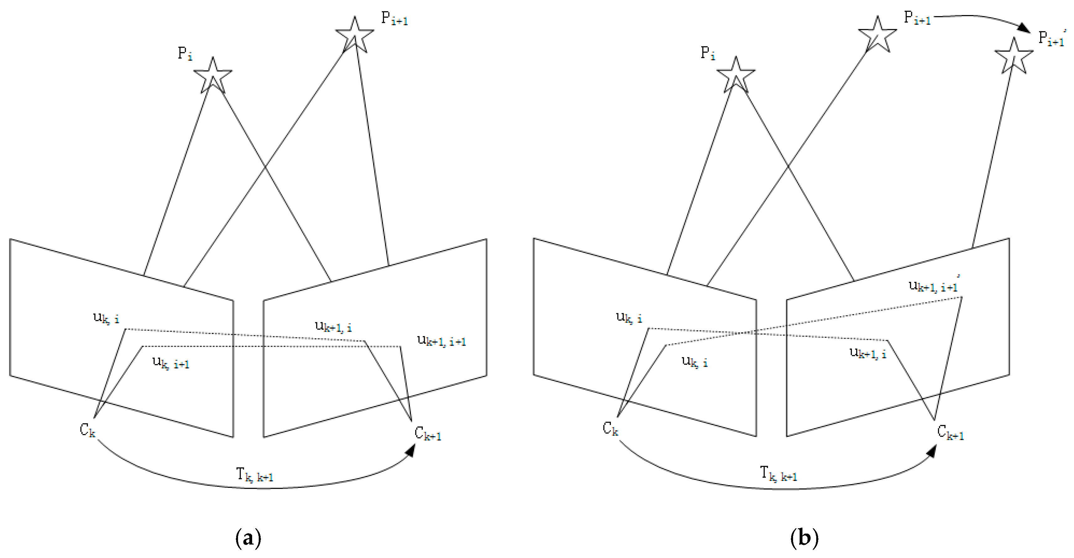
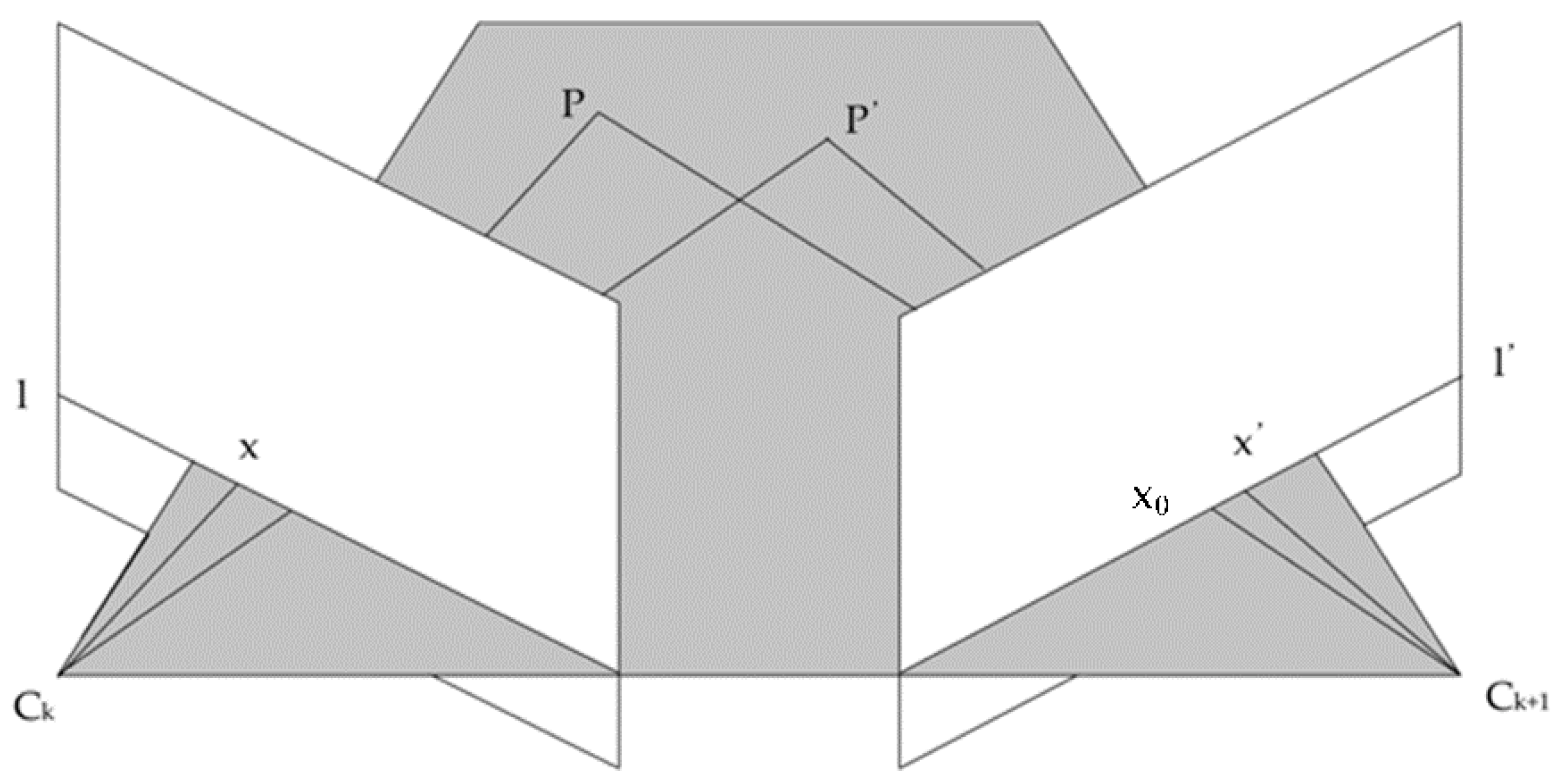
• FVB constraints were combined with IMU data. The motion model and epipolar were calculated using IMU data, and the dynamic feature point offset along the epipolar was eliminated using the FVB constraints.
• This method combined multiple constraints and used epipolar, FVB, GMS, and sliding window constraints, to compensate for the shortcomings of a single constraint and help VINS achieve more accurate feature matching.
• The proposed algorithm was integrated with VINS-mono, and VINS-dimc is proposed. We have conducted experiments with VINS-dimc.

The rest of the paper is organized as follows. First, in Section 2, the basic principle of VINS and the dynamic information feature point elimination algorithm based on multiple constraints are presented. Then, Section 3 presents the experimental scheme used in this study, the experimental procedure, and the results. Finally, Section 4 provides some discussion and concluding remarks.

2. Materials and Methods

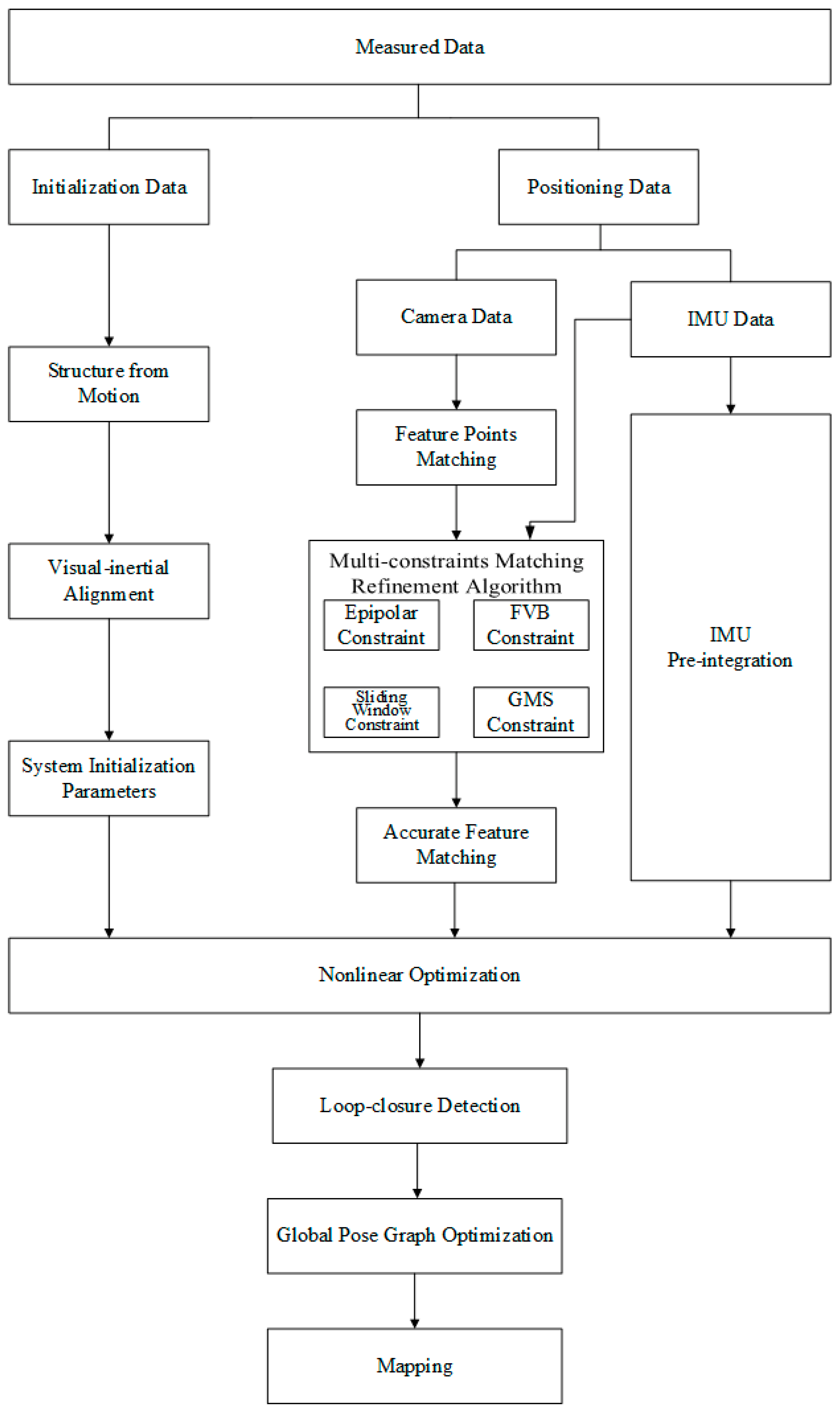
2.1. Overview

To improve the positioning accuracy of VINS in a dynamic environment, we propose a dynamic feature point elimination algorithm. It is integrated into VINS-mono, and a VINS-dimc with excellent performance in a dynamic environment is proposed. The flowchart of VINS-dimc is shown in Figure 2.

During the initialization stage, the system creates a local map through the structure from the movement. The initialization parameters of the system can be determined by aligning the IMU data with the visual data. The graph optimization method, based on bundle adjustment, is an important state estimation algorithm for the tight fusion of camera IMU data. The optimal solution is obtained by globally optimizing all the measurements [32,33]. The improvement in this study was in the feature point matching stage. Combining with the IMU data, we used a multi constraint dynamic feature point elimination algorithm to refine the feature point matching. The positioning accuracy of the system was improved by improving the accuracy of feature point matching.

2.2. IMU Data Validity Discrimination and Epipolar Constraint

The content of this part is similar to that of our previous study, so we will only briefly introduce it here. For further details, please refer to our earlier work.

Based on the position and attitude changes measured by IMU, the fundamental matrix of the camera motion can be obtained using the following formulas:

$${\mathit{E}}_{b_{k+1}}^c={\mathit{t}}_{b_{k+1}}^c{}^{\wedge }·{\mathit{R}}_{b_{k+1}}^c$$

(2)

$${\mathit{F}}_{b_{k+1}}^c={\mathit{K}}^{-T}·{\mathit{E}}_{b_{k+1}}^c·{\mathit{K}}^{-1}$$

(3)

where E is the essential matrix, ${\mathit{t}}^{\wedge }$ is the antisymmetric matrix of translation t, F is the fundamental matrix, and K is the intrinsic parameter of the camera.

The feature point on the previous frame image determines the epipolar line: ${\mathit{l}}^{\prime }=\mathit{F}\mathit{x}$. The distance between feature point matching and the fundamental matrix is calculated [34].

$$d=\frac{\left|{\mathit{p}}_{k+1,i}^T\mathit{F}{\mathit{p}}_{k,i}\right|}{\sqrt{{\mathit{x}}^2+{\mathit{y}}^2}},i=1, 2, 3, \dots , m$$

(4)

where

$$\mathit{F}{\mathit{p}}_{k,i}={[\mathit{x},\mathit{y},\mathit{z}]}^T$$

(5)

If the distance is less than threshold a, the feature matching will be consistent with the fundamental matrix; otherwise, it will be inconsistent. The value of ${\phi }_{k,i}$ is set to 0, when the ith feature point of the image frame is consistent; otherwise, it is set to 1, that is,

$${\phi }_{k,i}=\left\{\begin{array}{ll}1,& d_{k,i}\ge a\\ 0,& d_{k,i}<a\end{array}\right.$$

(6)

If the effective feature matches is not less than threshold b, the IMU data will be considered to be valid; otherwise, it is invalid. The value of ${\theta }_k$ is set to 0 when the the IMU data is invalid; otherwise, it is set to 1, that is,

$${\theta }_k=\left\{\begin{array}{ll}0,& {\displaystyle \sum _{i=1}^m}{\phi }_{k,i}<b\\ 1,& {\displaystyle \sum _{i=1}^m}{\phi }_{k,i}\ge b\end{array}\right..$$

(7)

If ${\theta }_k=1$, the fundamental matrix is accurate. The validity of feature point matching is determined by the distance between the matching and the fundamental matrix. If it is larger than the threshold c, it means that the feature matching differs from the motion model computed using the IMU data. This feature point matching is probably wrong or is on a dynamic object. Therefore, it is removed from the feature point matching set.

2.3. Multi Constraint Fusion Strategy

2.3.1. FVB Constraint

Epipolar constraints have shortcomings when the dynamic feature points move along the epipolar line as shown in Figure 3. Although point $\mathit{p}$ moves to point ${\mathit{p}}^{\prime }$, point ${\mathit{x}}^{\prime }$ is still on the epipolar line because point $\mathit{p}$ and point ${\mathit{p}}^{\prime }$ are in the same plane as the camera centers ${\mathit{c}}_k$ and ${\mathit{c}}_{k+1}$. In this case, the distance between the points and the epipolar line does not change. Therefore, the epipolar constraints are not valid.

To compensate for this situation, we introduced the FVB constraint. Let us assume that the translation of the camera is $t$. Let $\mathit{x}$ and ${\mathit{x}}^{\prime }$ be the corresponding pixels of the point $\mathit{p}$ and ${\mathit{p}}^{\prime }$ in the front and rear images, respectively. $z$ is the depth of the feature point in the scene. Then, the 3D coordinate of point $\mathit{p}$ is $z{\mathit{K}}^{-1}\mathit{x}$, and its coordinate in the image in the second image can be obtained using the following formulas:

$${\mathit{x}}_0=\mathit{K}[\mathit{I}|\mathit{t}]\mathit{p}$$

(8)

Since point P is moving, therefore,

$${\mathit{x}}^{\prime }-\mathit{x}=\mathit{K}\mathit{t}{z}^{-1}$$

(9)

When the camera moves, the corresponding pixels of the three-dimensional points in the image move along the line determined by the point ${\mathit{p}}_n$ and ${\mathit{e}}_{n+1}=\mathit{K}\mathit{t}$, and the amplitude of the motion depends on the translation amount $\mathit{t}$ and the depth $z$ [35].

We can specify a possible depth interval for 3D points and then determine the maximum and minimum displacements of the corresponding points on the epipolar line. If the displacement amplitude of a point is not between the minimum and maximum, it is probably a dynamic feature point.

If the IMU data is invalid (that is, ${\theta }_k=0$), we considered the accuracy of the translation $\mathit{t}$ calculated from the IMU data to be poor. Therefore, the FVB constraint was not used in such a case.

2.3.2. GMS Constraint

IMU datasets are not always accurate, and if the data has large deviation, the epipolar and FVB constraints are invalid. GMS constraints are required to prevent feature matching on a moving object.

We considered using spatial consistency between feature point matching to constrain the feature points. The constraint uses a grid-based motion statistics method, namely, GMS [36].

In this method, the statistical probability of some matches in a region is considered as the motion smoothness. Thus, all feature point matches are checked by the model to eliminate feature points on moving objects and to obtain a correct feature match. When feature points are matched, the GMS extracts high-quality feature matches to eliminate low-quality matches. This is an extremely robust matching method. Using video verification, even in a weak texture environment containing blurred images and wide baseline data, GMS has been found to consistently outperform other feature-matching algorithms that can be run in real time. GMS can achieve the same accuracy as more complex and slower algorithms. Since GMS has high accuracy and high execution speed, it is more suitable for use in VINSs.

We incorporated GMS constraints into a VINS system and used spatial consistency to eliminate feature point matching on dynamic objects.

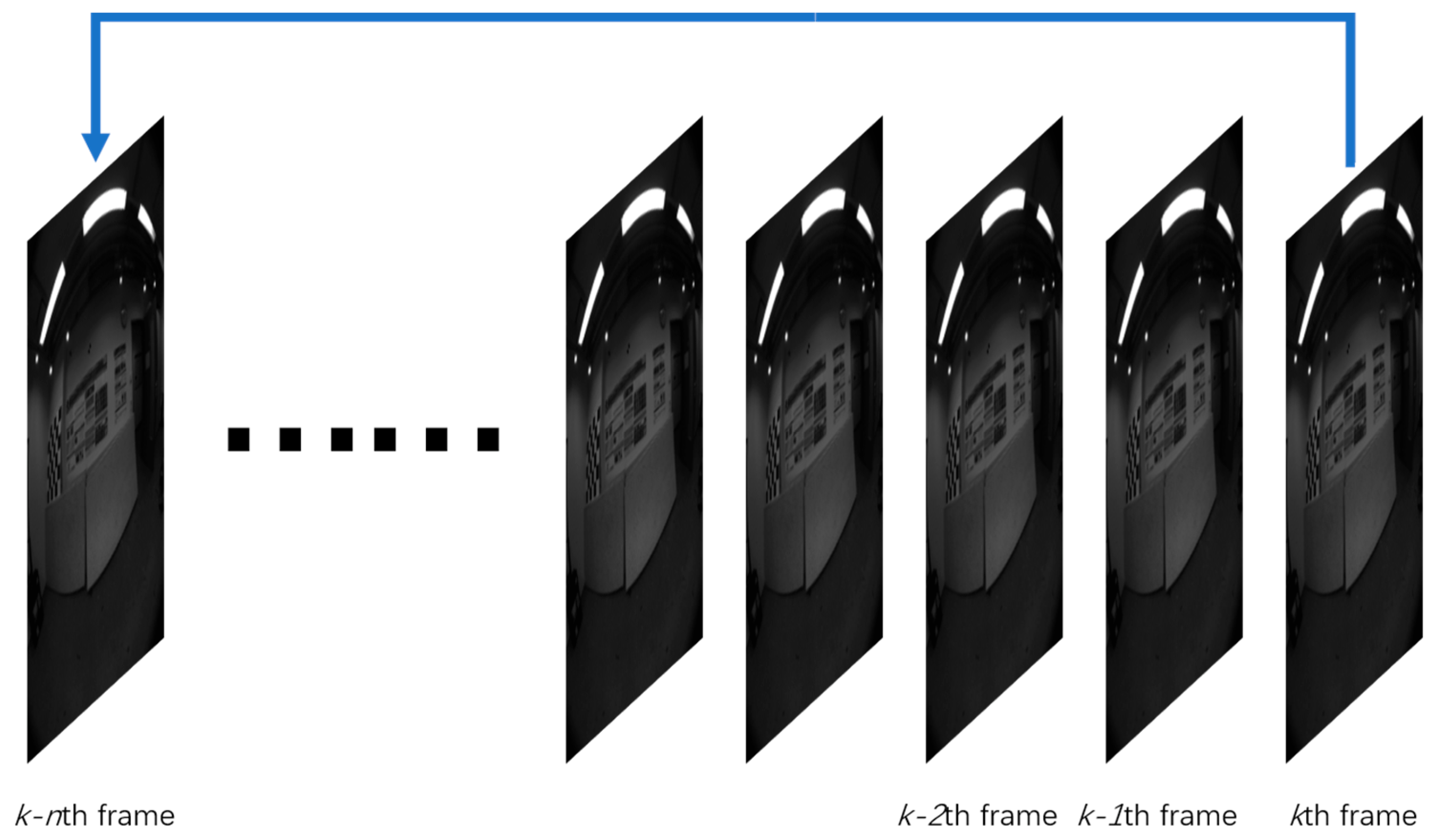
2.3.3. Sliding Window Constraint

In the VINS, which is based on the feature point method, two adjacent images are usually used for feature point matching to calculate the relative motion of the camera during this process. However, in a dynamic environment, we need to filter out dynamic feature points and maintain stationary matching, which is helpful for VINSs. However, due to the high frequency of the camera, which is usually more than 10 Hz, the pixels corresponding to the moving object do not have significant motion in the two adjacent images. Therefore, the VINS cannot reduce the influence of the moving object.

To solve this problem, the sliding window constraint was proposed to achieve feature matching between the current frame image and the image several frames before. The schematic representation of the sliding window constraint is as Figure 4.

When compared to the adjacent image frames, the time difference increases significantly. Therefore, the displacement of the pixels corresponding to the moving object in the two adjacent image frames becomes more obvious. However, the static feature points do not change. Thus, the influence of the dynamic object is reduced, and the features are matched to the static object.

2.3.4. Multi-Constraint Fusion Algorithm

Epipolar geometric constraints apply only to moving feature points that deviate from the epipolar line, whereas FVB constraints apply only to feature points that move along the epipolar line. These two constraints only matter when the accuracy of the IMU data is high. The GMS constraint restricts feature point matching by spatial consistency, and the sliding window constraint improves feature-matching accuracy by the temporal and spatial relationships of the visual data. These two constraints are independent of IMU data. Thus, the four feature-matching constraint algorithms can compensate each other. Therefore, the proposed algorithm integrates the above four constraints and avoids the failure of a single constraint.

3. Experiment

We integrated the multi constraint fusion algorithm proposed in this paper into VINS-mono, and proposed the VINS-dimc. An Intel(R) Core(TM) i7-7700hq CPU @ 2.80 GHz was used as the experimental platform. We performed the experiments on an Ubuntu 16.04 LTS system.

First, we verified the proposed algorithm by testing whether it could accurately eliminate dynamic feature matching by running the feature point matching experiment. Then, we ran the self-collected data into the VINSs to check whether it is helpful for positioning accuracy by checking the closed-loop error. Finally, we ran the public dataset in VINS-dimc. The positioning results were compared with the ground-truth to calculate the absolute positioning error. Then, the root mean square error (RMSE) of the error could be be obtained. We chose VINS-mono, OKVIS-mono, and ROVIO as references, which are among the most representative visual–inertial navigation systems. We also used our previous work as a reference to prove that this improvement is effective.

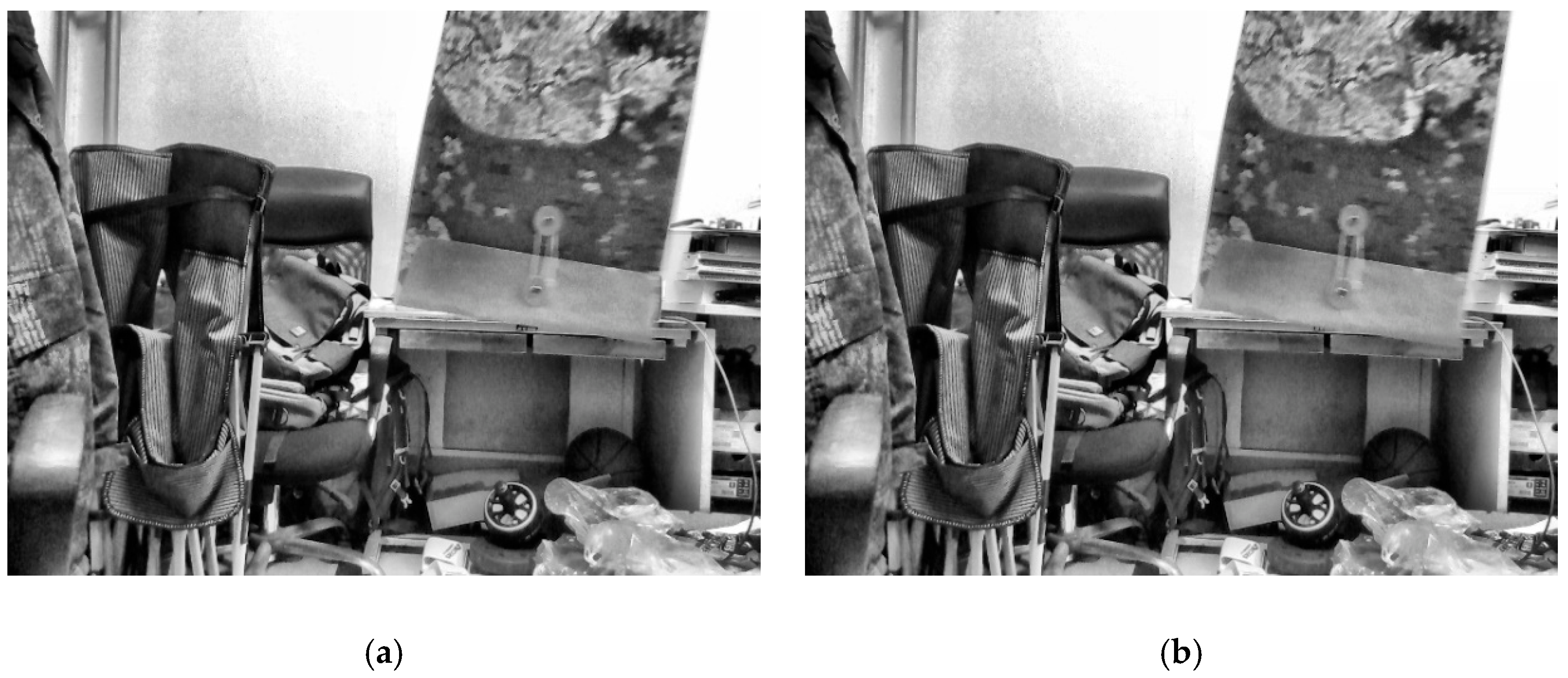
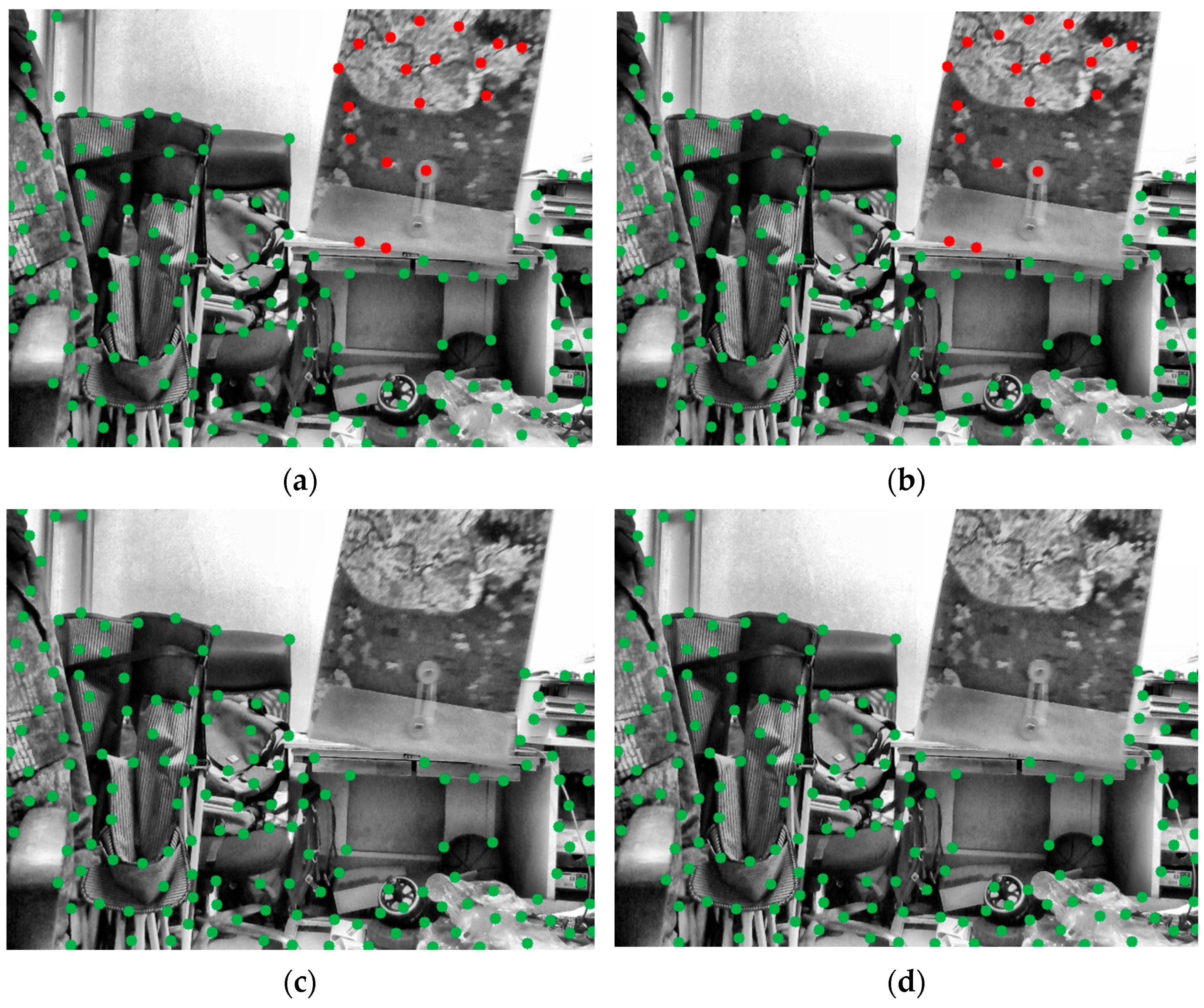
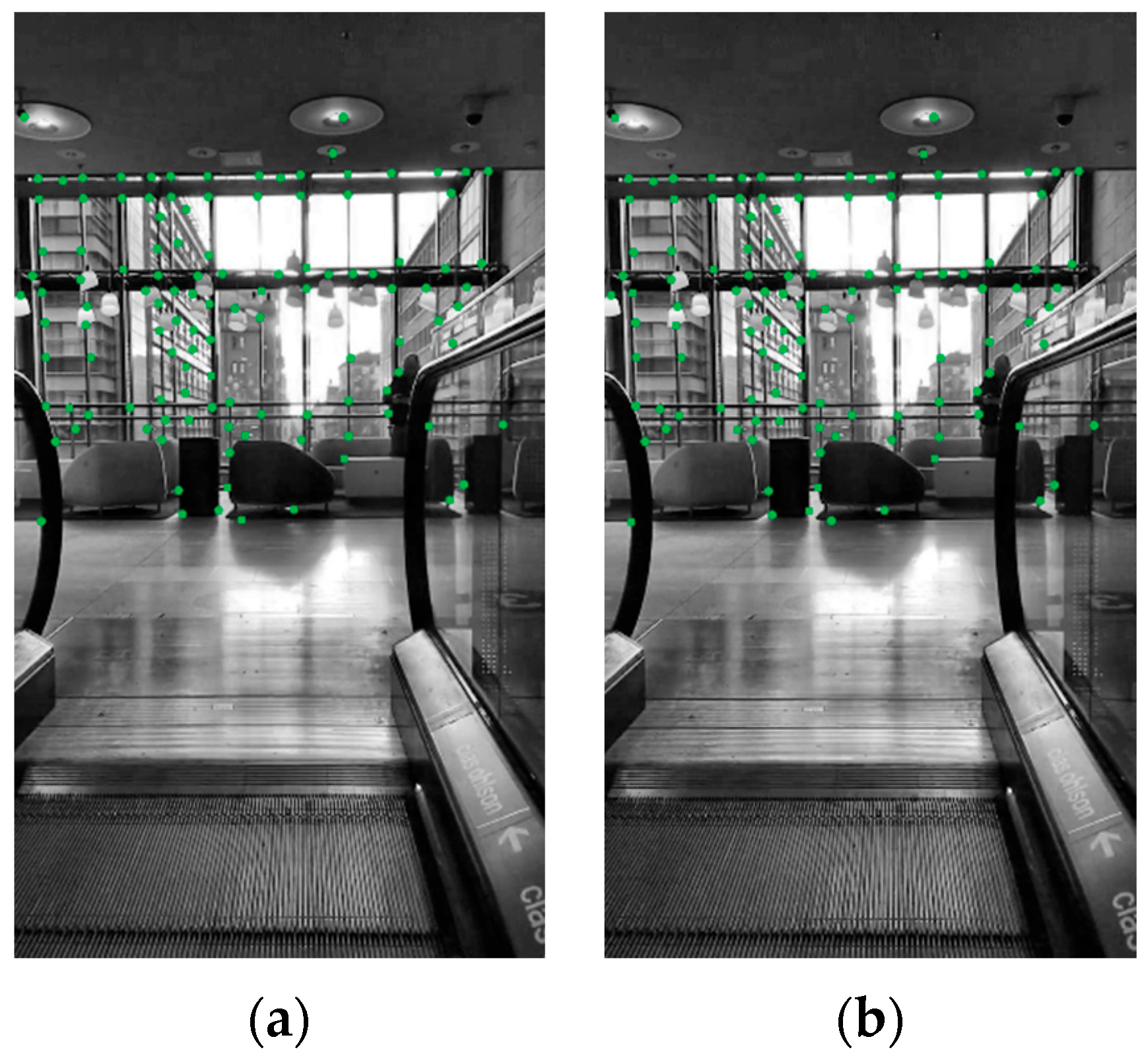
3.1. Feature Point Matching Experiment

3.1.1. Materials and Experimental Setup

The equipment we used for data acquisition was the Intel RealSense d435i camera [37]. It is a monocular camera with IMU and depth camera. Only RGB images and IMU data were used in this experiment. We set the resolution of the image data to 640 × 480, and the frequency to 15 Hz. The frequency of the accelerometer was set to 60 Hz, and the frequency of the gyroscope to 200 Hz.

During data acquisition, the experimenter shook the file bag in front of the lens. In the scene, the file bag is a moving object while the other objects are motionless. We used the traditional method and the proposed algorithm to perform the experiments. The collected image example is shown in Figure 5. Figure 5a is the image of the previous frame and Figure 5b is the image of the current frame.

3.1.2. Results

Since only the file bag is moving in the scene, the ideal result is that there are no moving points on the file bag. The results of feature point matching are shown in Figure 6. Figure 6a,b shows the results of feature matching using the traditional method, and Figure 6c,d shows the results of the proposed algorithm. In Figure 6a,b, there are many feature points on the moving portfolio. However, in the proposed method, there are no feature points on the moving file bag. The feature points on the static object are the same as those in the traditional method. Therefore, the proposed algorithm can effectively eliminate dynamic feature points.

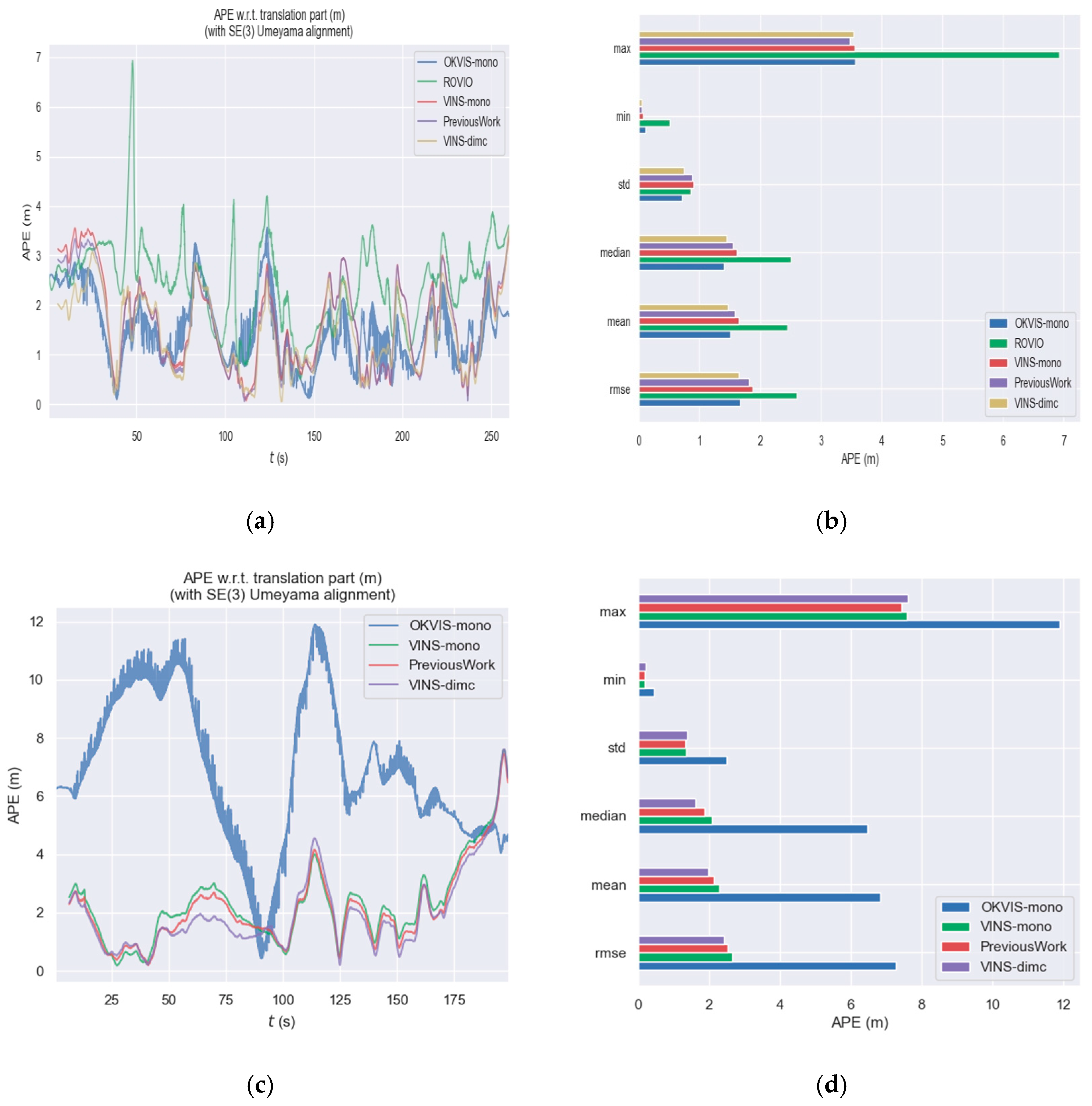
3.2. VINS Positioning Experiment

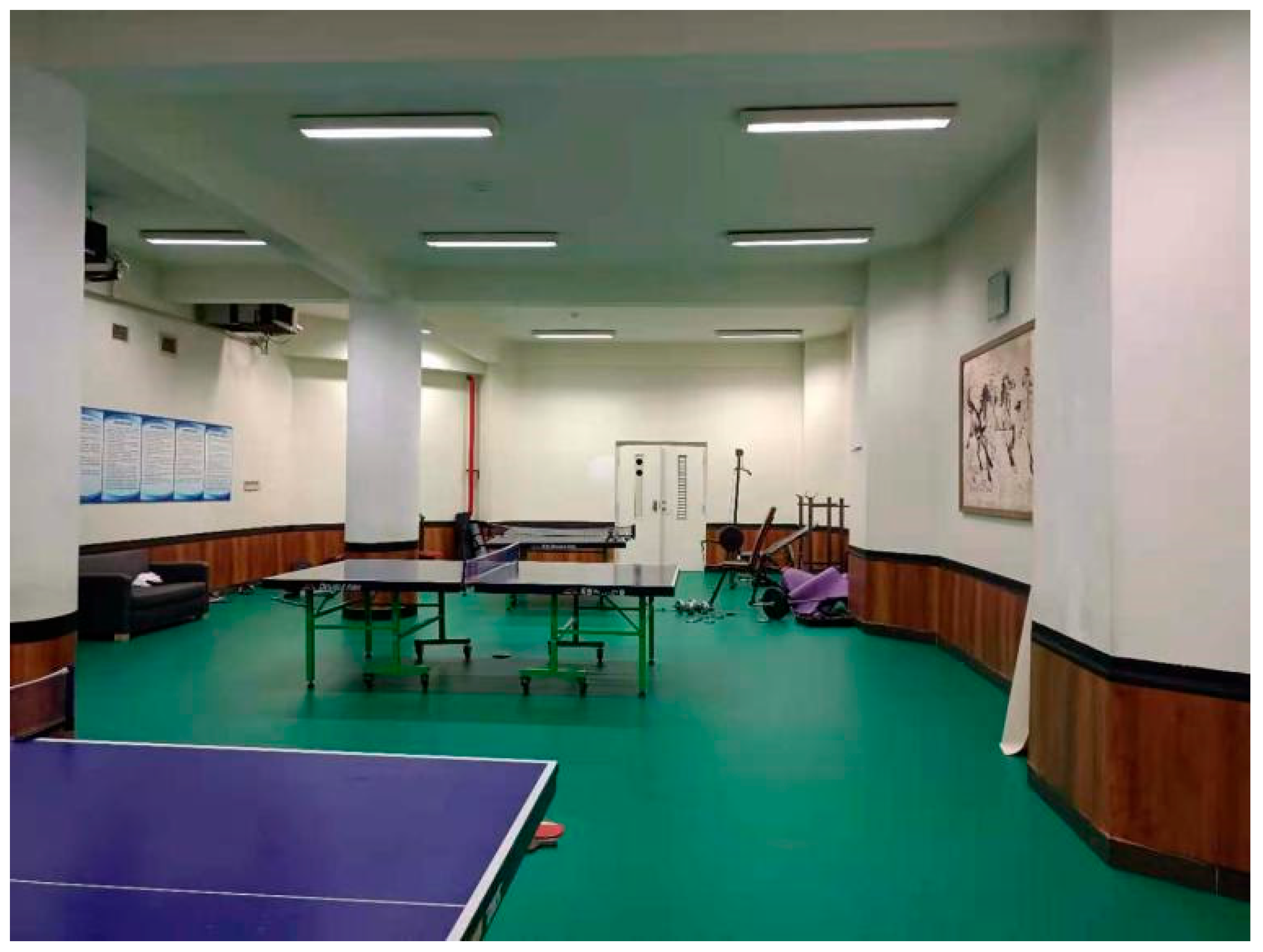
3.2.1. Materials and Experimental Setup

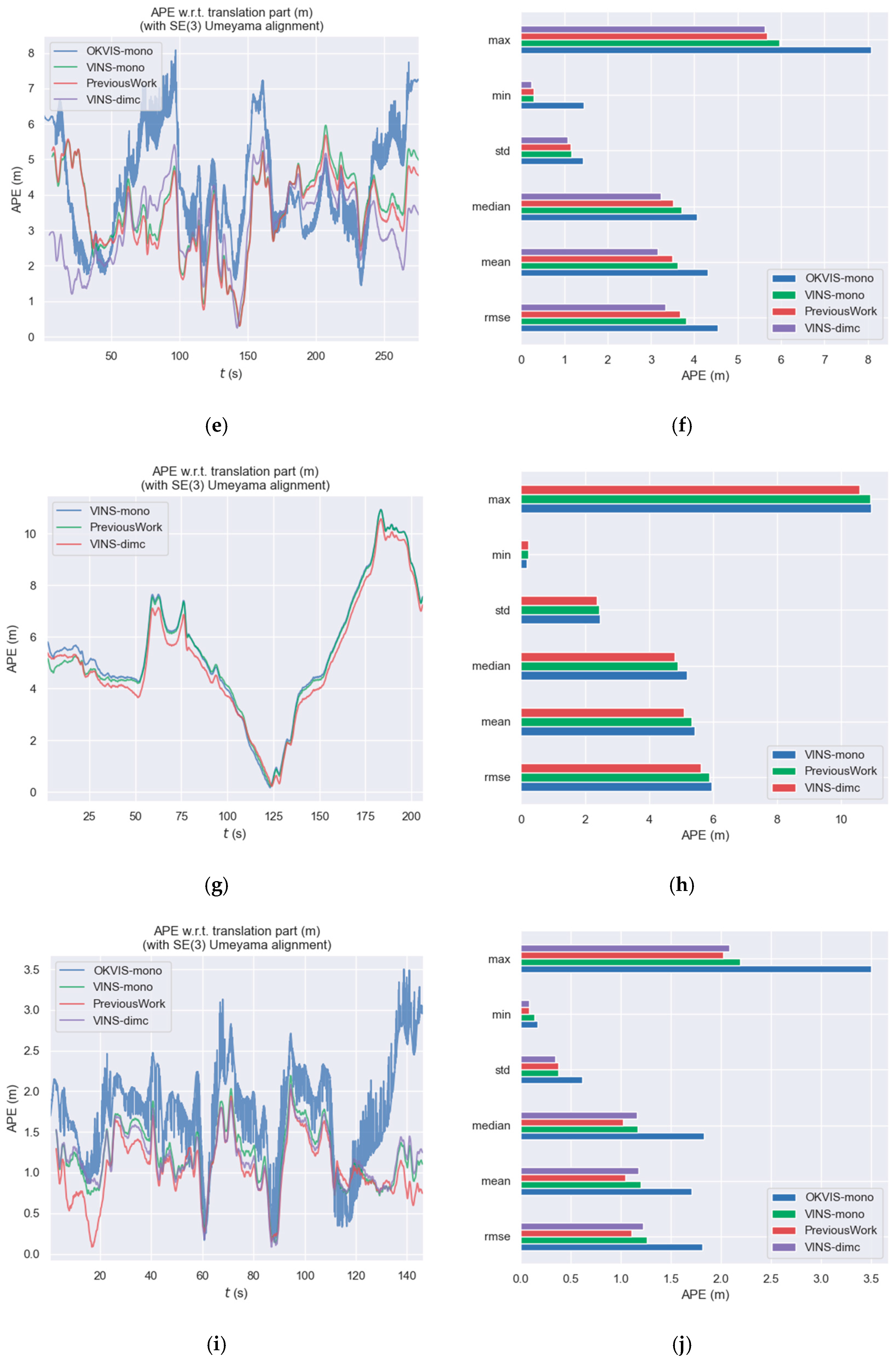
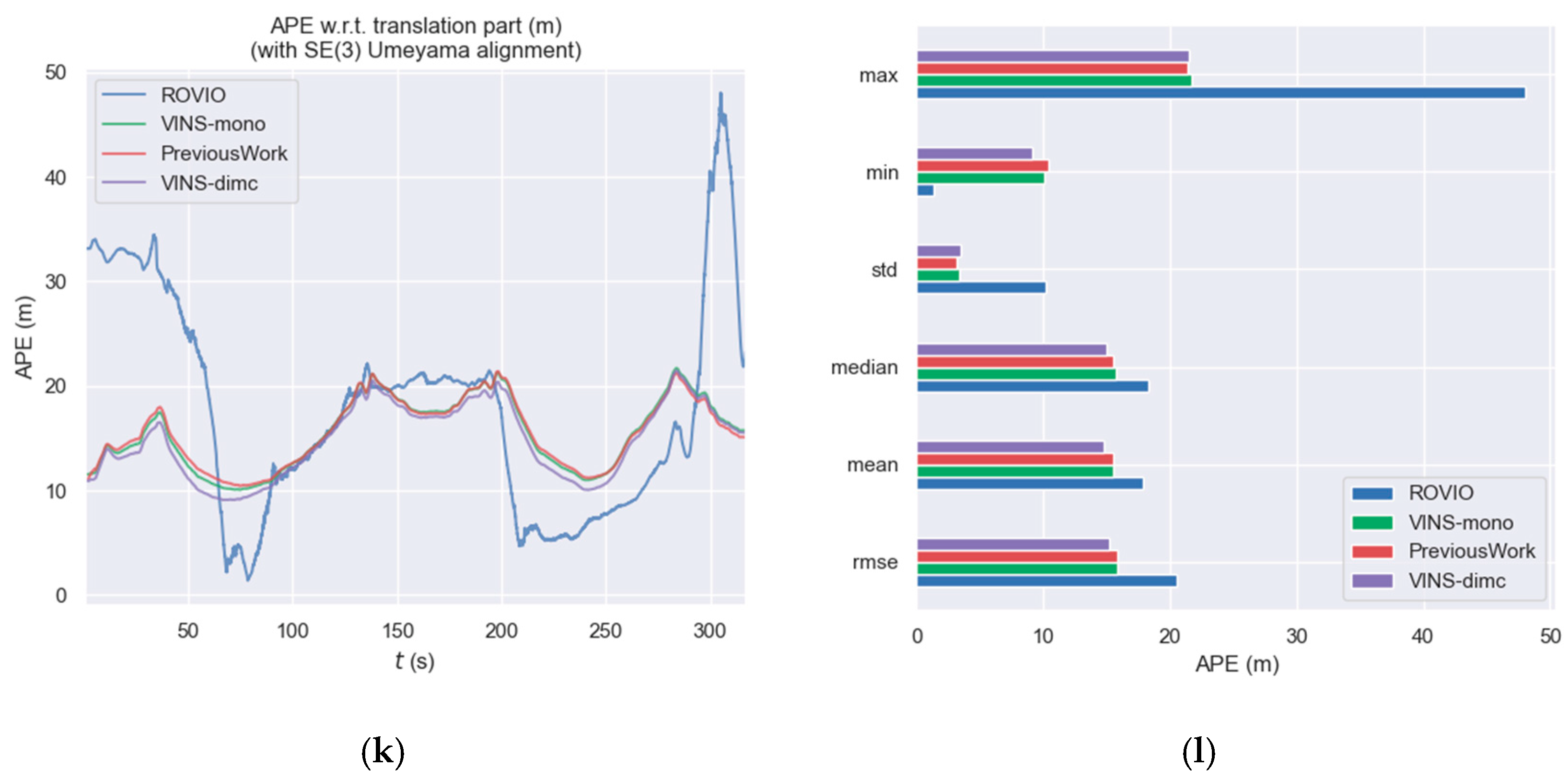
We performed an experimental verification using real scenes. The experimental scenario is shown in Figure 7. During the experiment, a person walked around the scene. Therefore, there is a certain amount of dynamic information in the scene, which is a challenge for the VINS system. Since there is no exact ground-truth, we set the start and end of the experiment to the same point, so that we could evaluate the positioning accuracy by comparing the deviation between the start and end. During the experiment, the experimenters held the camera to collect data along the closed-loop path in the scene.

In this experiment, the same camera was used to collect data as in the previous experiment. The data acquisition parameters were also the same as in the previous experiment. An example of the visual data for the two adjacent frames we captured is shown in Figure 8.

3.2.2. Results

We used the proposed algorithm to eliminate feature points on moving objects, and the feature-matching results are shown in Figure 9. Figure 9a,b show the distribution of the feature points. The experiment shows that the proposed algorithm is still effective in the VINSs. The algorithm was able to eliminate the feature points that are on the pedestrians and retain the feature points of the static scene.

We set the start and end points of the positioning experiment to the same position, and the difference between the positioning result at the last moment and the initial value can be considered as an index of accuracy.

Figure 10 shows the results of the experiment. Figure 10a shows the track of the system in 3D space. Figure 10b shows the changes of XYZ three-axis coordinates during the experiment. The positioning results of the three systems differed only slightly in the XY direction; however, the loop error of VINS-dimc in the Z-direction was much smaller than that of OKVIS-mono and VINS-mono.

We calculated the difference in positioning results between the end point and the start point. The difference in OKVIS-mono was 0.516 m and the difference in VINS-mono was 0.168 m, whereas the difference in VINS-dimc was 0.153 m.

Based on the proposed algorithm, the positioning accuracy of VINS-dimc improved significantly when compared to VINS-mono. So, the proposed algorithm is also effective for the self-collected data. The algorithm obviously contributes to positioning accuracy.

3.3. ADVIO Dataset Experiment

3.3.1. Materials and Experimental Setup

To scientifically test the positioning accuracy of VINS-dimc, we performed experiments on the ADVIO public dataset [38] with ground-truth. This is a public dataset that uses handheld devices for visual–inertial odometry, such as the sensors in a smartphone. The dataset contains 23 sequences that include recordings from both outdoor and indoor settings. The ground-truth is obtained by combining a recent pure inertial navigation system [39].

To verify the algorithm in different scenarios, this study selected the six most representative of the 23 sequences. The selected sequences were 1, 2, 6, 11, 16, and 21, which contain various experimental scenes, including a shopping mall, a subway station, an office, and an outdoor area. They also contain all kinds of dynamic objects, such as pedestrians, elevators, and moving cars.

Two adjacent raw images from sequence 1 of the public dataset were selected as shown in Figure 11. Figure 11a shows the previous image, and Figure 11b shows the current image. In these two image frames, the other objects are motionless except for the moving elevator. Therefore, only the moving elevator affects the feature matching. Therefore, the ideal result is that all feature points on the elevator are eliminated and the other feature points are retained.

3.3.2. Experimental Results

During the experiment, VINS extracts feature points and matches, and eliminates the abnormal features of the two images. We use the proposed feature point elimination algorithm in VINS. Figure 12 shows the feature points matching results. Figure 12a,b shows the distribution of feature points in the image.

The proposed algorithm is also suitable for public data sets. It can eliminate the feature points on the moving elevator while retaining other feature points, and there is no obvious error in feature matching.

We used the Evo library [40] to calculate the RMSE of the absolute positioning error (APE) of the positioning result. APE is the direct difference between the estimated pose and the ground-truth, which can directly reflect the accuracy of the algorithm and the global consistency of the trajectory. It should be noted that the estimated pose and ground truth are usually not in the same coordinate system, so we need to align them first. We need to calculate a transformation matrix $\mathrm{S}\in SE\left(3\right)$ from the estimated pose to the ground-truth using the least square method. Therefore, the APE of frame i is defined as follows:

$${\mathit{E}}_i={{\mathit{Q}}_i}^{-1}S{\mathit{P}}_i$$

(10)

where, $\mathit{Q}$ represents the ground-truth and $\mathit{P}$ represents the calculation result of the algorithm.

Then, use root mean squared error (RMSE) to count the APE:

$$RMSE\left({\mathit{E}}_{1:n},\Delta \right)={(\frac{1}{m}\sum _{i=1}^m\Vert trans{\left({\mathit{E}}_i\right)\Vert }^2)}^{\frac{1}{2}}$$

(11)

where ∆ represents the interval time and m represents the number of samples taken.

In the six sequences of the ADVIO public dataset, the error comparison data between the proposed method and the original method are shown in

Table 1. RMSE of results in different sequences in ADVIO dataset (unit in meters).

Sequence	Venue	Object	People	OKVIS-Mono	ROVIO	VINS-Mono	Previous Work	VINS-dimc
1	Mall	Escalator	Moderate	1.6606	2.5990	1.8393	1.8140	1.6428
2	Mall	None	Moderate	7.2727	-	2.5336	2.5160	2.4170
6	Mall	None	High	4.5450	-	3.8394	3.6688	3.3327
11	Metro	Vehicles	High	-	-	5.8722	5.8740	5.6198
16	Office	Stairs	None	1.8130	-	1.2584	1.1092	1.2231
21	Urban	Vehicles	Low	-	20.5237	15.8333	15.8889	15.1988

.

Since the dataset contains many dynamic objects that require the system to be highly robust, both OKVIS-mono and ROVIO are unable to run some of the datasets. As shown in Table 1, VINS-dimc achieved excellent performance when compared to the other three state-of-the-art VINSs. When compared to our previous work, VINS-dimc has also made significant progress. Not only are there scenes with considerable dynamic information, but also scenes where almost all objects are stationary, such as in an office. The system not only runs successfully for all datasets, but also improves the positioning accuracy. VINS-dimc achieves better robustness and higher positioning accuracy than conventional VINSs in both dynamic and static environments.

Figure 13 shows the error data of the results for different sequences in the ADVIO public dataset. The figures in the left column show the absolute error over time. The abscissa represents the experimental time; the unit is seconds, and the ordinate is the absolute position error in meters. The figures in the right column show the statistics for the absolute position error. The statistics in the figures from top to bottom are the maximum, minimum, standard deviation, median, mean, and RMSE. The horizontal axis represents the size in meters.

4. Discussion and Conclusions

In this study, we present an algorithm for feature-matching elimination based on multiple constraints. This algorithm has two main advantages. First, the information from IMU is combined with epipolar and FVB constraints to eliminate abnormal feature points using geometric relationships. Second, the GMS and sliding window constraints are introduced, which are combined with the epipolar and FVB constraints to eliminate feature point matching for dynamic objects. The Epipolar constraint and FVB constraint combine IMU data and use geometric information to eliminate dynamic feature points. The GMS constraint considers the spatial consistency of the feature point matching. Sliding window constraint uses time correlation to constrain feature points. Thus, the proposed algorithm integrates four constraints to avoid the failure of a single constraint.

We integrated the algorithm into VINS-mono and proposed VINS-dimc. Through feature point matching experiments, we proved that the proposed algorithm is helpful in removing dynamic feature points. In the experiment with self-collected data, the closed-loop error of VINS-dimc is much lower than that of conventional methods. In the experiment with the ADVIO public dataset, the positioning error of VINS-dimc is the smallest. Therefore, the proposed method can improve the matching accuracy of feature points and the positioning accuracy of VINSs.

In future work, we will consider another difficulty of VINS: illumination changes. In practical applications, the change of illumination has a great impact on the stability of feature points. We intend to propose an image enhancement method and integrate it with VINS to improve the accuracy and robustness of the system.

References

1. Alliez, P.; Bonardi, F.; Bouchafa, S.; Didier, J.-Y.; Hadj-Abdelkader, H.; Muñoz, F.I.I.; Kachurka, V.; Rault, B.; Robin, M.; Roussel, D. Real-time multi-SLAM system for agent localization and 3D mapping in dynamic scenarios. In Proceedings of the International Conference on Intelligent Robots and Systems, Las Vegas, NV, USA, 24–30 October 2020; IROS: Las Vegas, NV, USA, 2020. [Google Scholar]
2. Ram, K.; Kharyal, C.; Harithas, S.S.; Krishna, K.M. RP-VIO: Robust plane-based visual-inertial odometry for dynamic environments. arXiv 2021, arXiv:2103.10400. [Google Scholar]
3. Bonin-Font, F.; Ortiz, A.; Oliver, G. Visual navigation for mobile robots: A survey. J. Intell. Robot. Syst. 2008, 53, 263–296. [Google Scholar] [CrossRef]
4. Yang, D.; Bi, S.; Wang, W.; Yuan, C.; Wang, W.; Qi, X.; Cai, Y. DRE-SLAM: Dynamic RGB-D encoder SLAM for a differential-drive robot. Remote Sens. 2019, 11, 380. [Google Scholar] [CrossRef] [Green Version]
5. Sibley, G.; Mei, C.; Reid, I.; Newman, P. Vast-scale outdoor navigation using adaptive relative bundle adjustment. Int. J. Robot. Res. 2010, 29, 958–980. [Google Scholar] [CrossRef]
6. Yang, S.; Scherer, S.A.; Yi, X.; Zell, A. Multi-camera visual SLAM for autonomous navigation of micro aerial vehicles. Robot. Auton. Syst. 2017, 93, 116–134. [Google Scholar] [CrossRef]
7. Gao, Q.H.; Wan, T.R.; Tang, W.; Chen, L.; Zhang, K.B. An improved augmented reality registration method based on visual SLAM. In E-Learning and Games; Lecture Notes in Computer Science; Springer: Cham, Switzerland, 2017; pp. 11–19. [Google Scholar]
8. Mahmoud, N.; Grasa, Ó.G.; Nicolau, S.A.; Doignon, C.; Soler, L.; Marescaux, J.; Montiel, J. On-patient see-through augmented reality based on visual SLAM. Int. J. Comput. Assist. Radiol. Surg. 2017, 12, 1–11. [Google Scholar] [CrossRef]
9. Qin, T.; Li, P.; Shen, S. Vins-Mono: A robust and versatile monocular visual-inertial state estimator. IEEE Trans. Robot. 2018, 34, 1004–1020. [Google Scholar] [CrossRef] [Green Version]
10. Leutenegger, S.; Lynen, S.; Bosse, M.; Siegwart, R.; Furgale, P. Keyframe-based visual–inertial odometry using nonlinear optimization. Int. J. Robot. Res. 2015, 34, 314–334. [Google Scholar] [CrossRef] [Green Version]
11. Bloesch, M.; Omari, S.; Hutter, M.; Siegwart, R. Robust visual inertial odometry using a direct EKF-based approach. In Proceedings of the 2015 IEEE/RSJ International Conference on Intelligent Robots and Systems (IROS), Hamburg, Germany, 28 September–2 October 2015; pp. 298–304. [Google Scholar]
12. Mourikis, A.I.; Roumeliotis, S.I. A multi-state constraint Kalman filter for vision-aided inertial navigation. In Proceedings of the 2007 IEEE International Conference on Robotics and Automation, Roma, Italy, 10–14 April 2007; pp. 3565–3572. [Google Scholar]
13. Geneva, P.; Eckenhoff, K.; Lee, W.; Yang, Y.; Huang, G. Openvins: A research platform for visual-inertial estimation. In Proceedings of the 2020 IEEE International Conference on Robotics and Automation, Paris, France, 31 May–31 August 2020; pp. 4666–4672. [Google Scholar]
14. Wang, R.; Wan, W.; Wang, Y.; Di, K. A new RGB-D SLAM method with moving object detection for dynamic indoor scenes. Remote Sens. 2019, 11, 1143. [Google Scholar] [CrossRef] [Green Version]
15. Cheng, J.; Sun, Y.; Meng, M.Q.-H. Improving monocular visual SLAM in dynamic Environments: An Optical-Flow-Based Approach. Adv. Robot. 2019, 33, 576–589. [Google Scholar] [CrossRef]
16. Shimamura, J.; Morimoto, M.; Koike, H. Robust vSLAM for dynamic scenes. In Proceedings of the MVA, Nara, Japan, 6–8 June 2011; Volume 2011, pp. 344–347. [Google Scholar]
17. Tan, W.; Liu, H.; Dong, Z.; Zhang, G.; Bao, H. Robust monocular SLAM in dynamic environments. In Proceedings of the 2013 IEEE International Symposium on Mixed and Augmented Reality (ISMAR), Adelaide, Australia, 1–4 October 2013; Volume 2013, pp. 209–218. [Google Scholar]
18. Rünz, M.; Agapito, L. Co-Fusion: Real-time segmentation, tracking and fusion of multiple objects. In Proceedings of the 2017 IEEE International Conference on Robotics and Automation (ICRA), Singapore, 29 May 2017; pp. 4471–4478. [Google Scholar]
19. Sun, Y.; Liu, M.; Meng, M.Q.-H. Improving RGB-D SLAM in dynamic environments: A motion removal approach. Robot. Auton. Syst. 2017, 89, 110–122. [Google Scholar] [CrossRef]
20. Alcantarilla, P.F.; Yebes, J.J.; Almazán, J.; Bergasa, L.M. On combining visual SLAM and dense scene flow to increase the robustness of localization and mapping in dynamic environments. In Proceedings of the 2012 IEEE International Conference on Robotics and Automation, Bielefeld, Germany, 13–17 August 2012; Volume 2012, pp. 1290–1297. [Google Scholar]
21. Lee, D.; Myung, H. Solution to the SLAM problem in low dynamic environments using a pose graph and an RGB-D sensor. Sensors 2014, 14, 12467–12496. [Google Scholar] [CrossRef]
22. Li, A.; Wang, J.; Xu, M.; Chen, Z. DP-SLAM: A visual SLAM with moving probability towards dynamic environments. Inf. Sci. 2021, 556, 128–142. [Google Scholar] [CrossRef]
23. Nam, D.V.; Gon-Woo, K.J.S. Robust stereo visual inertial navigation system based on multi-stage outlier removal in dynamic environments. Sensors 2020, 20, 2922. [Google Scholar] [CrossRef]
24. Wang, Y.; Huang, S. Towards dense moving object segmentation based robust dense RGB-D SLAM in dynamic scenarios. In Proceedings of the 2014 13th International Conference on Control Automation Robotics & Vision (ICARCV), Singapore, 10–12 December 2014; Volume 2014, pp. 1841–1846. [Google Scholar]
25. Yang, S.; Scherer, S. Cubeslam: Monocular 3-D Object Slam. IEEE Trans. Robot. 2019, 35, 925–938. [Google Scholar] [CrossRef] [Green Version]
26. Bescos, B.; Fácil, J.M.; Civera, J.; Neira, J. DynaSLAM: Tracking, mapping, and inpainting in dynamic scenes. IEEE Robot. Autom. Lett. 2018, 3, 4076–4083. [Google Scholar] [CrossRef] [Green Version]
27. Yu, C.; Liu, Z.; Liu, X.-J.; Xie, F.; Yang, Y.; Wei, Q.; Fei, Q. DS-SLAM: A semantic visual SLAM towards dynamic environments. In Proceedings of the 2018 IEEE/RSJ International Conference on Intelligent Robots and Systems (IROS), Madrid, Spain, 1–5 October 2018; pp. 1168–1174. [Google Scholar]
28. Brasch, N.; Bozic, A.; Lallemand, J.; Tombari, F. Semantic monocular SLAM for highly dynamic environments. In Proceedings of the 2018 IEEE/RSJ International Conference on Intelligent Robots and Systems (IROS), Madrid, Spain, 1–5 October 2018; Volume 2018, pp. 393–400. [Google Scholar]
29. Jiao, J.; Wang, C.; Li, N.; Deng, Z.; Xu, W. An adaptive visual dynamic-SLAM method based on fusing the semantic information. IEEE Publ. Sens. J. 2021. [Google Scholar] [CrossRef]
30. Zhang, C.; Huang, T.; Zhang, R.; Yi, X. PLD-SLAM: A new RGB-D SLAM method with point and line features for indoor dynamic scene. Inf. Sci. 2021, 10, 163. [Google Scholar] [CrossRef]
31. Fu, D.; Xia, H.; Qiao, Y. Monocular visual-inertial navigation for dynamic environment. Remote Sens. 2021, 13, 1610. [Google Scholar] [CrossRef]
32. Mur-Artal, R.; Tardós, J.D.; Letters, A. visual-inertial monocular SLAM with map reuse. IEEE Robot. Autom. Lett. 2017, 2, 796–803. [Google Scholar] [CrossRef] [Green Version]
33. Yang, Z.; Shen, S. Monocular visual–inertial state estimation with online initialization and camera–IMU extrinsic calibration. IEEE Trans. Robot. 2016, 14, 39–51. [Google Scholar] [CrossRef]
34. Hartley, R.; Zisserman, A. Multiple View Geometry in Computer Vision; Cambridge University Press: Cambridge, UK, 2003. [Google Scholar]
35. Kundu, A.; Krishna, K.M.; Sivaswamy, J. Moving object detection by multi-view geometric techniques from a single camera mounted robot. In Proceedings of the 2009 IEEE/RSJ International Conference on Intelligent Robots and Systems, St. Louis, MO, USA, 10–15 October 2009; Volume 2009, pp. 4306–4312. [Google Scholar]
36. Bian, J.; Lin, W.; Liu, Y.; Zhang, L.; Yeung, S.; Cheng, M.; Reid, I. GMS: Grid-based motion statistics for fast, ultra-robust feature correspondence. Int. J. Comput. Vis. 2020, 128, 1580–1593. [Google Scholar] [CrossRef] [Green Version]
37. Intel. RealSense. Available online: https://www.intelrealsense.com/depth-camera-d435i (accessed on 28 September 2020).
38. Cortés, S.; Solin, A.; Rahtu, E.; Kannala, J. ADVIO: An authentic dataset for visual-inertial odometry. In Proceedings of the European Conference on Computer Vision (ECCV), Munich, Germany, 8–14 September 2018; pp. 425–440. [Google Scholar]
39. Solin, A.; Cortes, S.; Rahtu, E.; Kannala, J. Inertial odometry on handheld smartphones. In Proceedings of the 2018 21st International Conference on Information Fusion (Fusion), Cambridge, UK, 10–13 July 2018; Volume 2018, pp. 1–5. [Google Scholar]
40. Grupp, M. Evo: Python Package for the Evaluation of Odometry and SLAM. Available online: https://github.com/MichaelGrupp/evo (accessed on 20 April 2021).
Figure 1. Schematic diagrams of (a) static environments and (b) dynamic environments feature point matching. (a) Shows a situation in where the feature point is stationary, (b) shows a situation where the feature point p i is stationary, whereas the feature point p i + 1 is moving. c k and c k + 1 represent the center of the camera at two points in time. T k , k + 1 is the motion of the camera during the period from time point k to time point k + 1. The rectangles represent the imaging plane of the camera. u k , i represents the imaging of the i-th feature point at time point k.
Ijgi 11 00095 g001
Figure 2. Flowchart of VINS-dimc using our proposed algorithm.
Ijgi 11 00095 g002
Figure 3. Schematic representation of the failure of epipolar constraints. c k and c k + 1 are the center of the camera, point p moves to point p , l and l are epipolar lines. Two parallelograms represent the imaging plane of the camera. x and x are the points in the image. The four points P , P , C k and C k + 1 are coplanar.
Ijgi 11 00095 g003
Figure 4. Schematic diagram of the sliding window constraint. The feature points of the current frame image are matched with the feature points of the previous nth image.
Ijgi 11 00095 g004
Figure 5. Two adjacent images: (a) the previous and (b) current image frames.
Ijgi 11 00095 g005
Figure 6. Results of feature point matching. (a,b) Results of the traditional methods. (c,d) Results of the proposed algorithm. (a,c) Feature point distribution of the previous frame. (b,d) Feature point distribution of the next frame. Green points are static feature points and red points are dynamic feature points.
Ijgi 11 00095 g006
Figure 7. Experiment scene for data collection.
Ijgi 11 00095 g007
Figure 8. Visual data of two adjacent frames: (a) the previous and (b) current image frames.
Ijgi 11 00095 g008
Figure 9. The results of feature point matching using the proposed algorithm. (a) Feature point distribution map of the previous frame image, and (b) feature point distribution map of the current frame image. Green points are static feature points.
Ijgi 11 00095 g009
Figure 10. Positioning experiment results of the self-collected visual data: (a) Positioning track in 3D space and (b) variation of XYZ 3D coordinates during the experiment duration.
Ijgi 11 00095 g010
Figure 11. Two adjacent image in the ADVIO dataset: (a) the previous image, (b) the current image.
Ijgi 11 00095 g011
Figure 12. Feature point matching results. (a) Feature point distribution map of the previous frame image, and (b) feature point distribution map of the current frame image. Green points are static feature points.
Ijgi 11 00095 g012
Figure 13. Comparison of positioning results between conventional OKVIS-mono, ROVIO, VINS-mono, previous works, and the proposed VINS-dimc on different sequences of the ADVIO dataset: (a,b) sequence 1, (c,d) sequence 2, (e,f) sequence 6, (g,h) sequence 11, (i,j) sequence 16, and (k,l) sequence 21. The left images show the absolute positioning error over time. The right images show some statistics on the absolute positioning error.
Ijgi 11 00095 g013aIjgi 11 00095 g013bIjgi 11 00095 g013c