
Toward Gaze-Based Map Interactions: Determining the Dwell Time and Buffer Size for the Gaze-Based Selection of Map Features


Abstract
:1. Introduction
2. Background and Related Work
2.1. Gaze-Based Interactions in HCI
2.2. Gaze-Based Interactions in Geo-Application
3. Method
3.1. Participants
3.2. Apparatus and Software
3.3. Parameter Values to Be Tested
3.4. Stimuli and Tasks
3.5. Procedure
- The calibration session. The participants were first welcomed and were seated in front of a laptop in a comfortable position. They were given a brief introduction to eye tracking, and then a 6-point calibration method was used to calibrate the participants’ eyes for the eye tracker. The calibration process was repeated during the experiment when necessary.
- The training session. The participants had at least five minutes to learn how to interact with the computer using their gazes; they practiced with the demos provided by Tobii. They were then required to finish five training tasks to ensure that they were familiar with the experimental procedure.
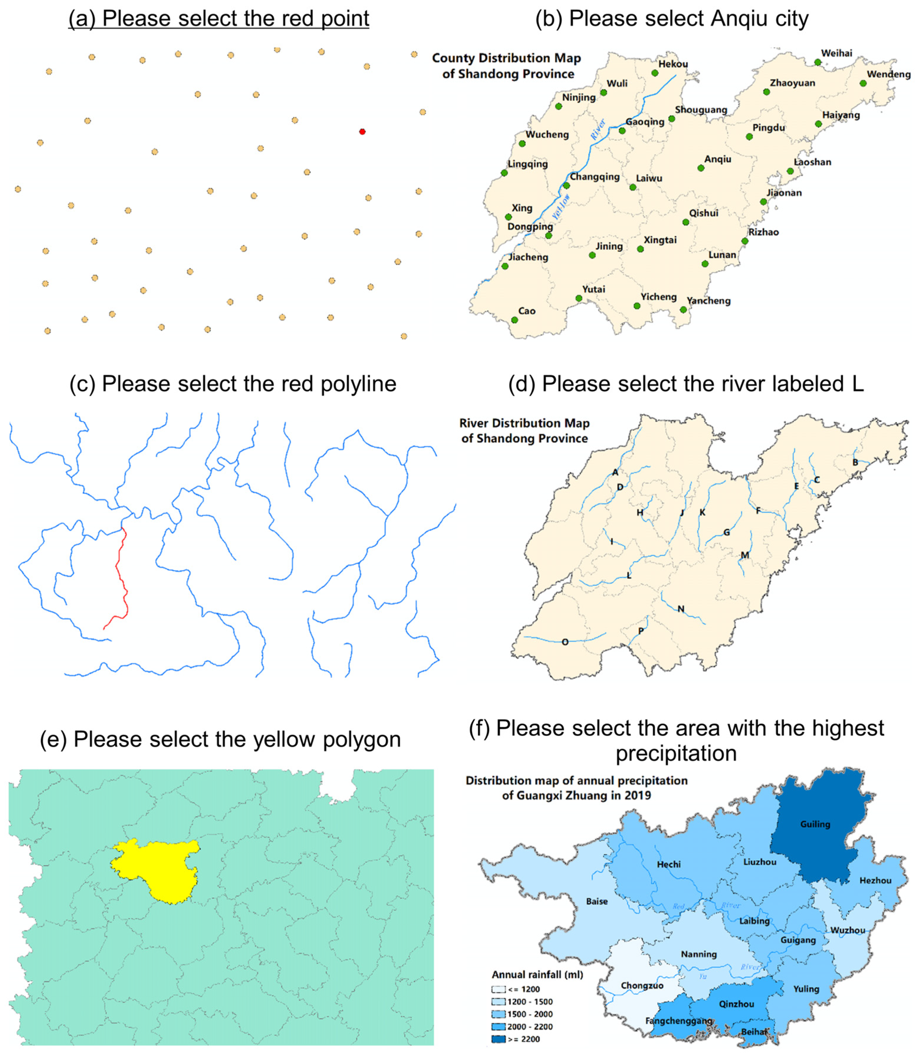
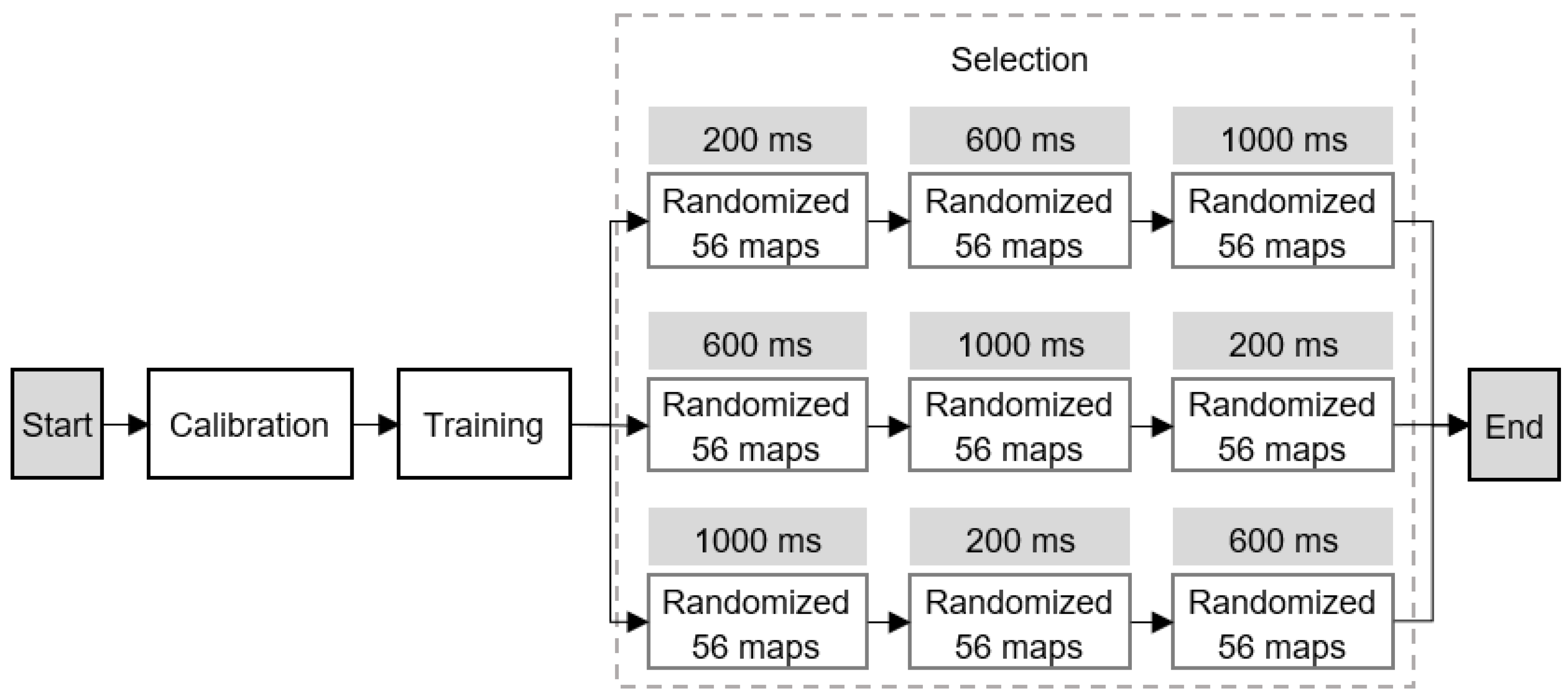
- The selection session. In this session, the participants were required to finish 168 tasks. We used a within-subject design, which means that all participants were presented with all maps. Each map was repeated with different combinations of buffer sizes and dwell times. To counter the learning effect, we adopted a Latin square-based order to present the tasks (see Figure 6). In each task, the task instruction was presented on the screen (Figure 7a). The participants were allowed to switch to the map interface by pressing the space bar after reading and understanding the task instruction correctly (Figure 7b). At this point, the participants needed to select the required map feature using their gaze. Any feature satisfying the parameter thresholds (see Section 3.3) was selected (highlighted in Figure 7c). Once they selected the required target, they were required to press the space bar to submit it as their final answer as soon as possible. To avoid the impact of the break-offs (e.g., participants’ phone call or the accidental disconnection of eye tracker) during the experiment, participants could press the enter key to skip the task. Whether the participant pressed the space bar or the enter key, the next task instruction would be presented (Figure 7d), but the skipped tasks would not be counted into the results.
3.6. Analysis
3.6.1. Data Quality Check
3.6.2. Evaluation Metric
4. Results
4.1. Point Selection
4.1.1. General Performance of Efficiency and Accuracy
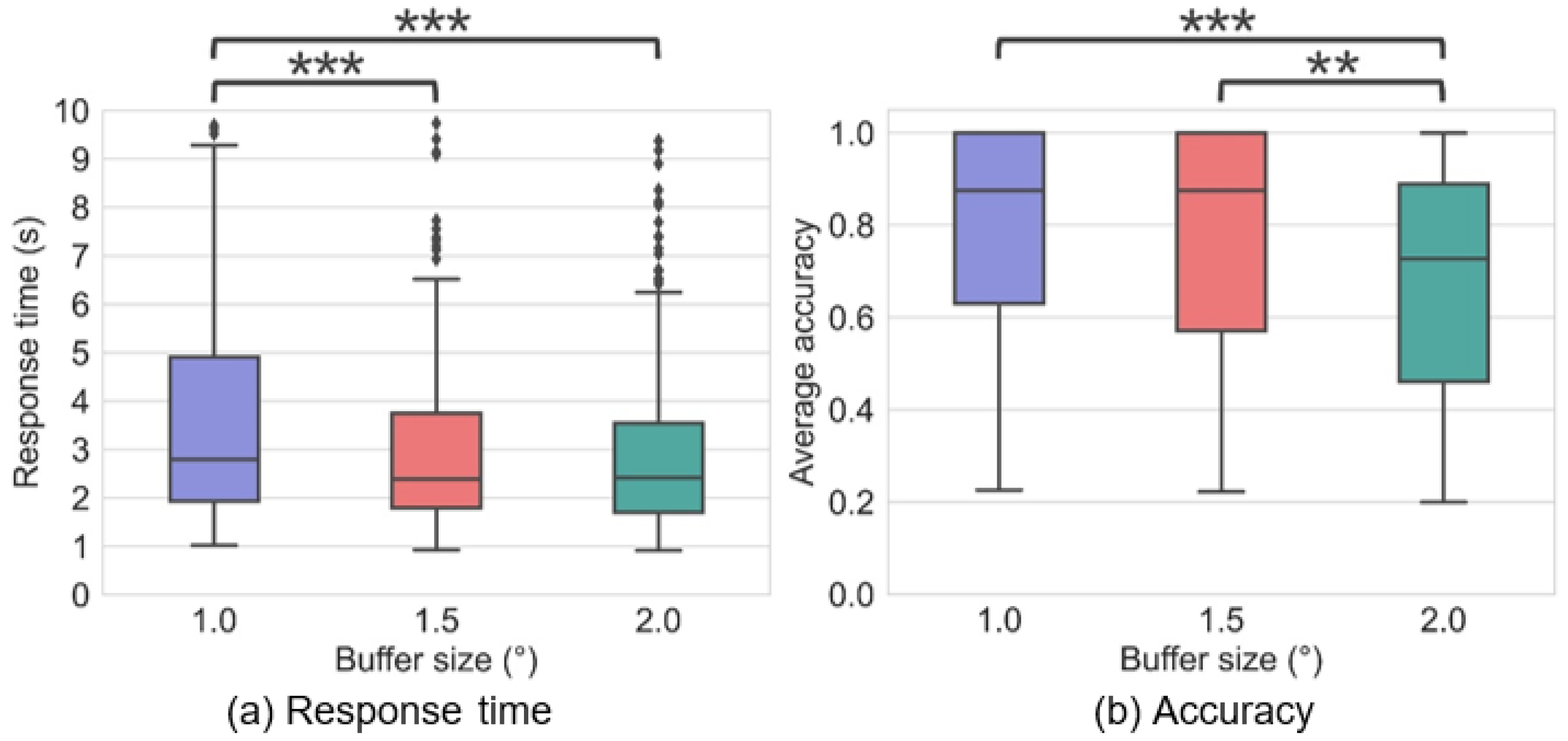
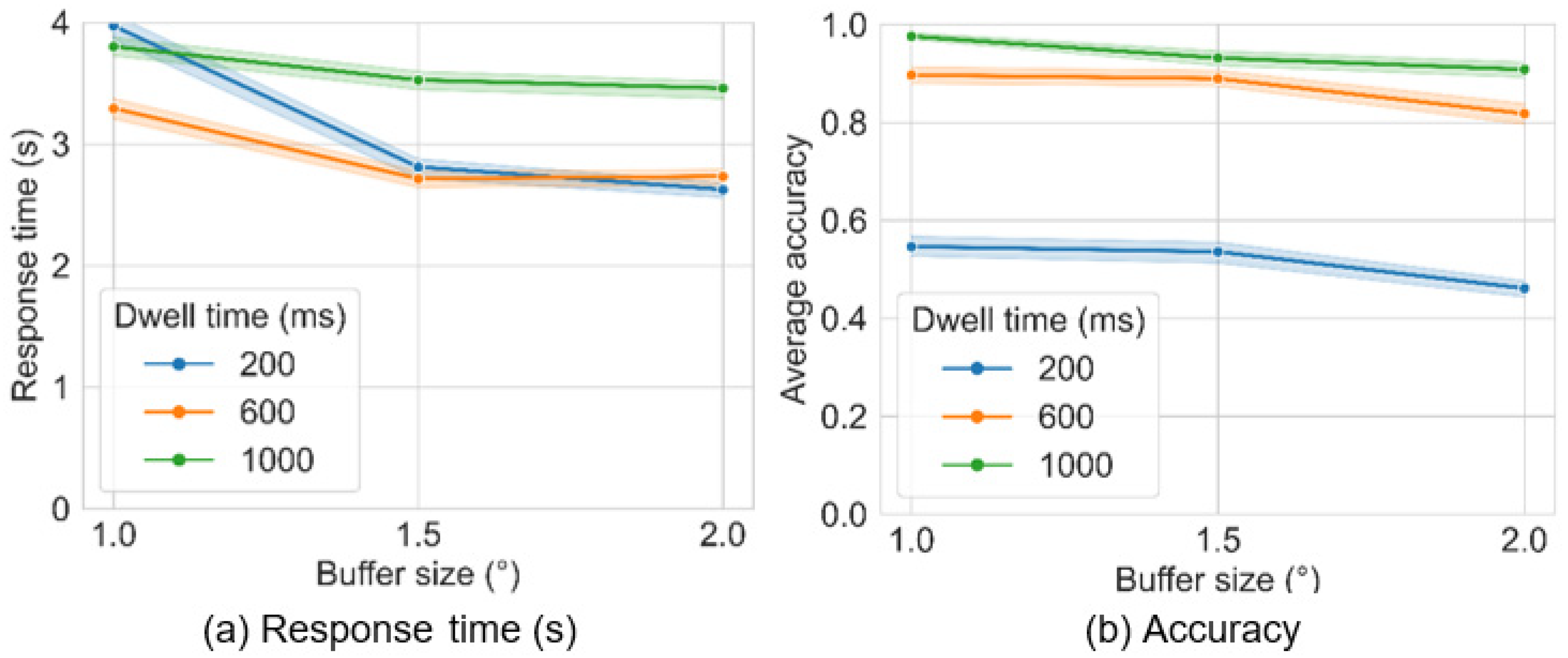
4.1.2. Effects of Buffer Size on Efficiency and Accuracy
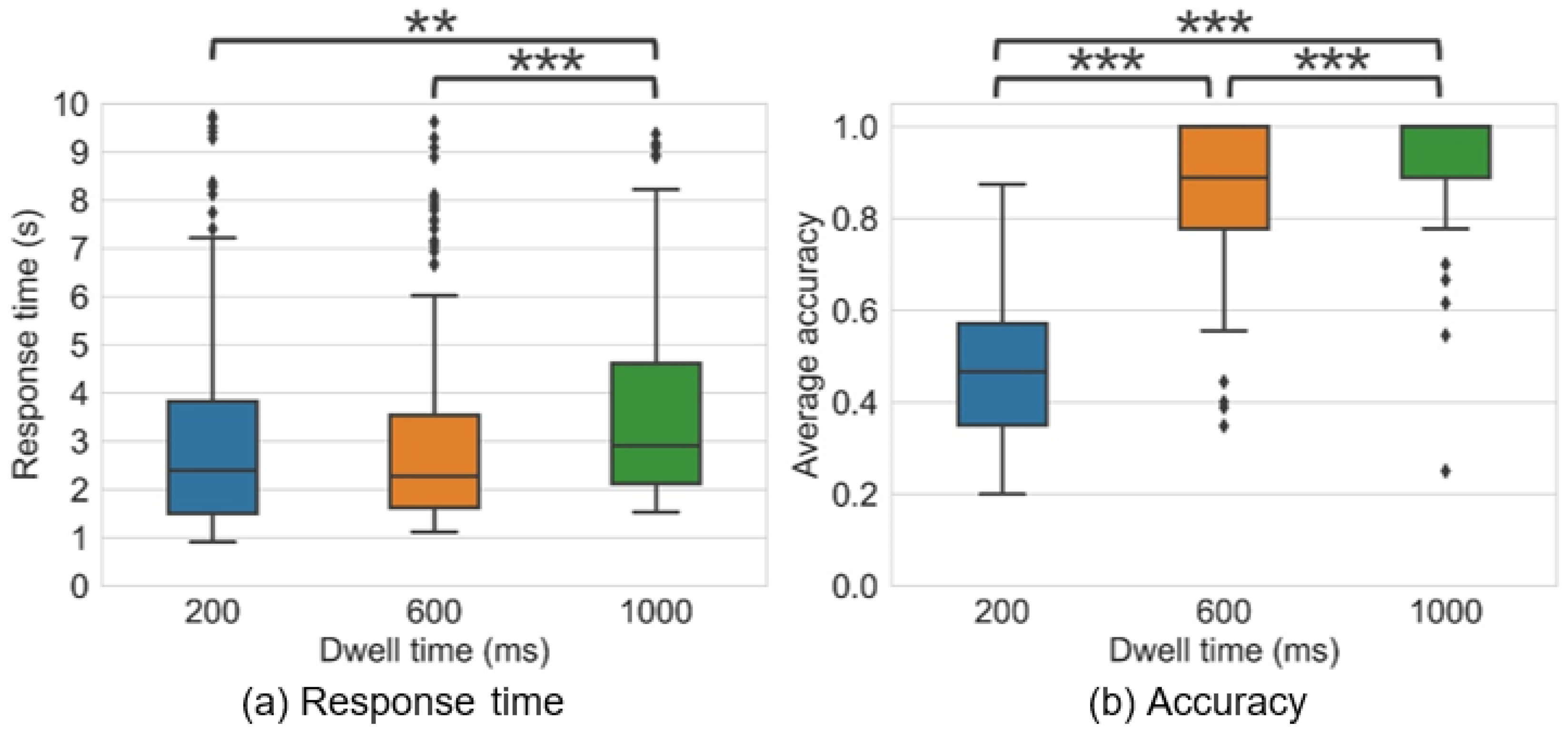
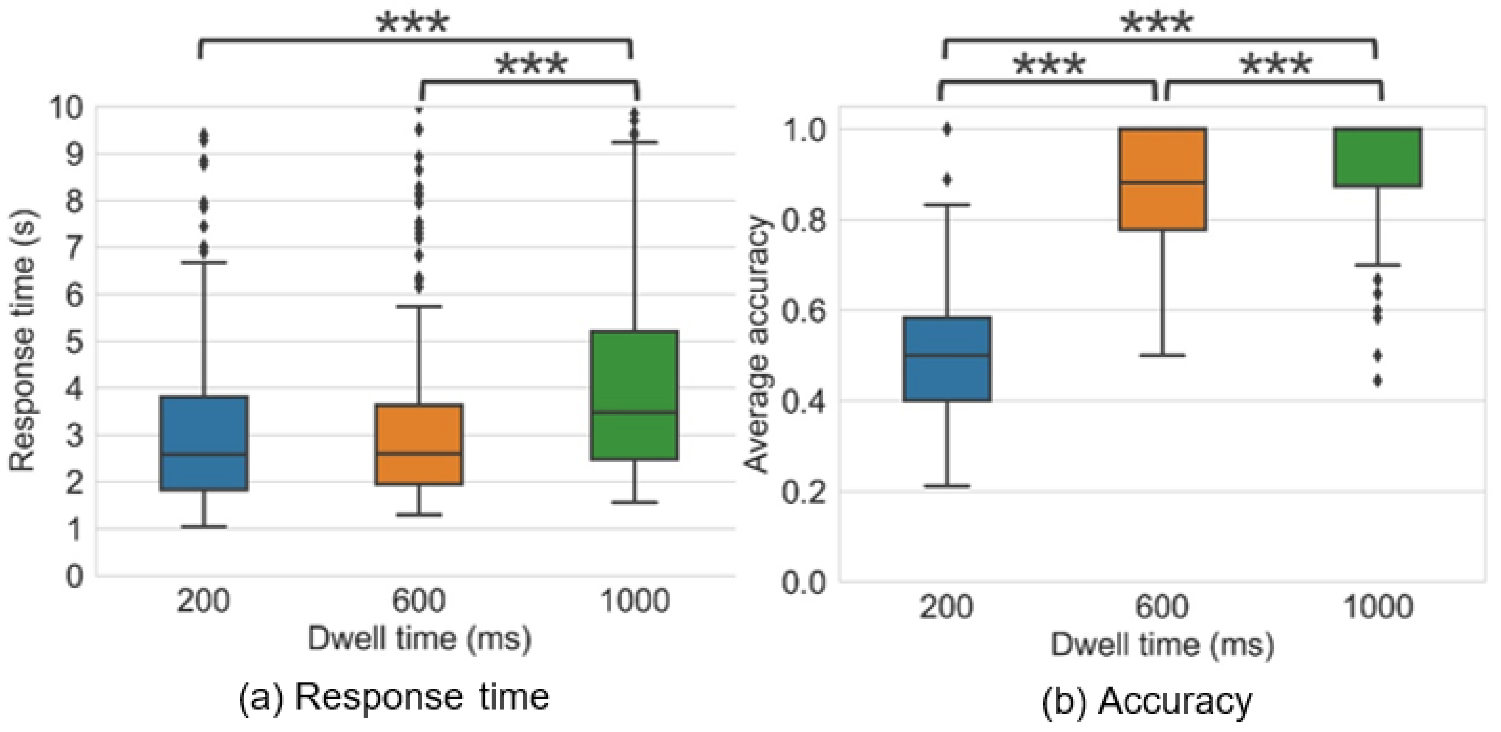
4.1.3. Effects of Dwell Time on Efficiency and Accuracy
4.2. Polyline Selection
4.2.1. General Performance of Efficiency and Accuracy
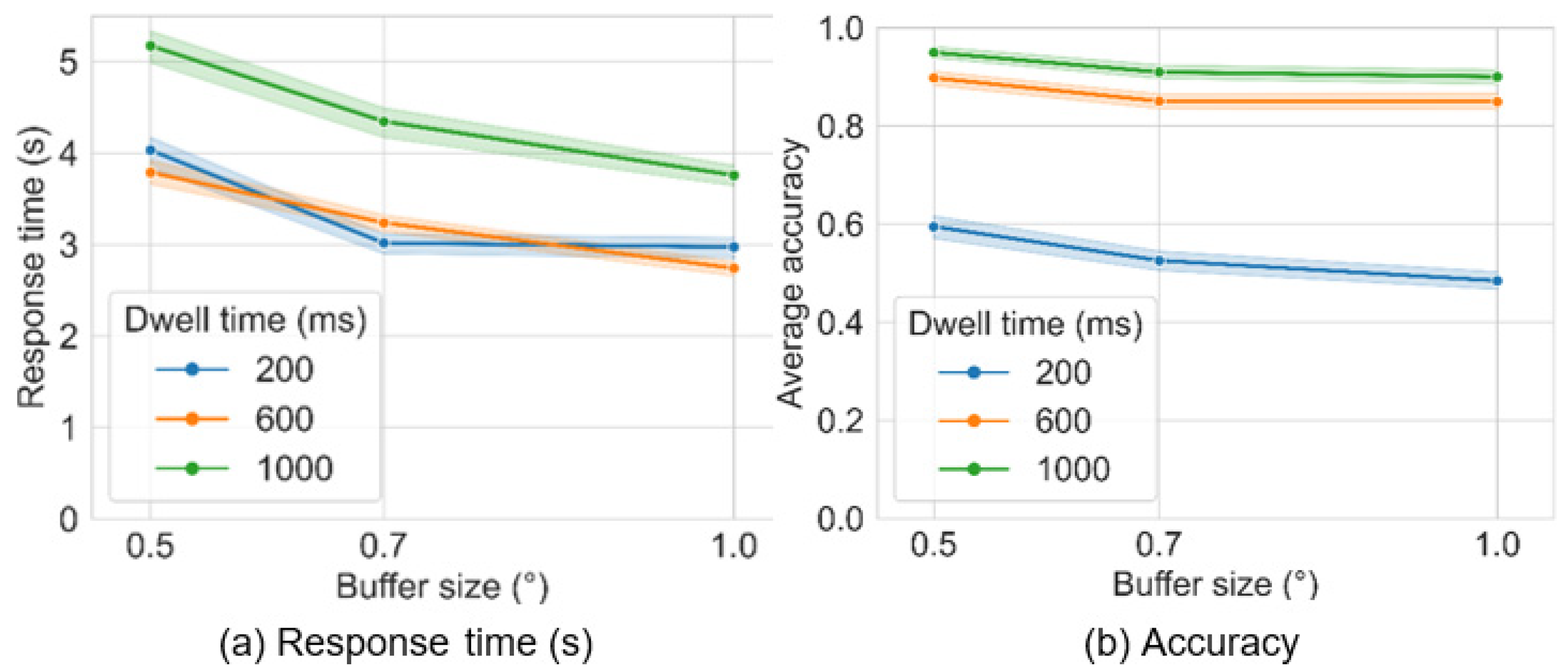
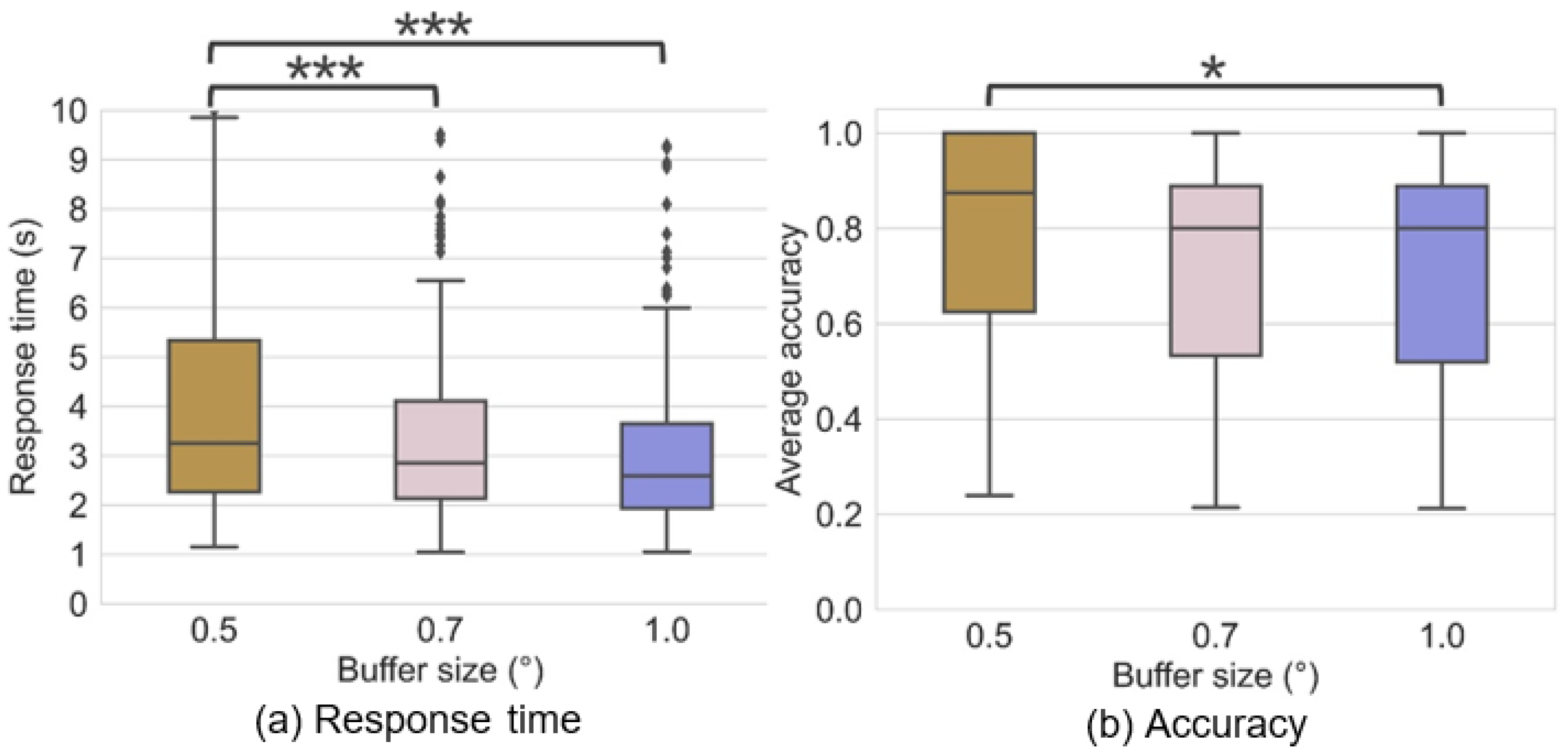
4.2.2. Effects of Buffer Size on Efficiency and Accuracy
4.2.3. Effects of Dwell Time on Efficiency and Accuracy
4.3. Polygon Selection
5. Discussion
5.1. Choosing the Appropriate Dwell Time and Buffer Size
5.1.1. Buffer Size
5.1.2. Dwell Time
5.2. Limitaions
6. Conclusions and Future Work
Author Contributions
Funding
Institutional Review Board Statement
Informed Consent Statement
Acknowledgments
Conflicts of Interest
References
- Newbury, R.; Satriadi, K.A.; Bolton, J.; Liu, J.; Cordeil, M.; Prouzeau, A.; Jenny, B. Embodied gesture interaction for immersive maps. Cartogr. Geogr. Inf. Sci. 2021, 48, 417–431. [Google Scholar] [CrossRef]
- Göbel, F.; Bakogioannis, N.; Henggeler, K.; Tschümperlin, R.; Xu, Y.; Kiefer, P.; Raubal, M. A Public Gaze-Controlled Campus Map. In Eye Tracking for Spatial Research, Proceedings of the 3rd International Workshop, Zurich, Switzerland, 14 January 2018; ETH Zurich: Zurich, Switzerland, 2018. [Google Scholar]
- Kiefer, P.; Zhang, Y.; Bulling, A. The 5th international workshop on pervasive eye tracking and mobile eye-based interaction. In International Symposium on Wearable Computers; Kenji Mase, M.L., Gatica-Perez, D., Eds.; ACM: New York, NY, USA, 2015; pp. 825–828. [Google Scholar]
- Chuang, L.; Duchowski, A.; Qvarfordt, P.; Weiskopf, D. Ubiquitous Gaze Sensing and Interaction (Dagstuhl Seminar 18252). In Dagstuhl Reports; Schloss Dagstuhl-Leibniz-Zentrum fuer Informatik: Wadern, Germany, 2019. [Google Scholar] [CrossRef]
- Kwok, T.C.K.; Kiefer, P.; Schinazi, V.R.; Adams, B.; Raubal, M. Gaze-Guided Narratives: Adapting Audio Guide Content to Gaze in Virtual and Real Environments. In CHI’ 19: Proceedings of the 2019 CHI Conference on Human Factors in Computing Systems; Stephen Brewster, G.F., Ed.; ACM: New York, NY, USA, 2019. [Google Scholar]
- Liao, H.; Dong, W.; Zhan, Z. Identifying Map Users with Eye Movement Data from Map-Based Spatial Tasks: User Privacy Concerns. Cartogr. Geogr. Inf. Sci. 2022, 49, 50–69. [Google Scholar] [CrossRef]
- Hayashida, N.; Matsuyama, H.; Aoki, S.; Yonezawa, T.; Kawaguchi, N. A Gaze-Based Unobstructive Information Selection by Context-Aware Moving UI in Mixed Reality. In International Conference on Human-Computer Interaction; Springer: Cham, Switzerland, 2021; pp. 301–315. [Google Scholar]
- Benabid Najjar, A.; Al-Wabil, A.; Hosny, M.; Alrashed, W.; Alrubaian, A. Usability Evaluation of Optimized Single-Pointer Arabic Keyboards Using Eye Tracking. Adv. Hum. Comput. Interact. 2021, 2021, 6657155. [Google Scholar] [CrossRef]
- Rudnicki, T. Eye-Control Empowers People with Disabilities. Available online: https://www.abilities.com/community/assistive-eye-control.html (accessed on 21 December 2021).
- Yi, J.S.; ah Kang, Y.; Stasko, J.T.; Jacko, J.A. Toward a Deeper Understanding of the Role of Interaction in Information Visualization. IEEE Trans. Vis. Comput. Graph. 2007, 13, 1224–1231. [Google Scholar] [CrossRef] [Green Version]
- Roth, R.E. An empirically-derived taxonomy of interaction primitives for interactive cartography and geovisualization. Vis. Comput. Graph. IEEE Trans. 2013, 19, 2356–2365. [Google Scholar] [CrossRef]
- Kasprowski, P.; Harezlak, K.; Niezabitowski, M. Eye movement tracking as a new promising modality for human computer interaction. In Proceedings of the 2016 17th International Carpathian Control Conference (ICCC), High Tatras, Slovakia, 29 May–1 June 2016; pp. 314–318. [Google Scholar]
- Niu, Y.; Gao, Y.; Zhang, Y.; Xue, C.; Yang, L. Improving eye–computer interaction interface design: Ergonomic investigations of the optimum target size and gaze-triggering dwell time. J. Eye Mov. Res. 2019, 12, 1–14. [Google Scholar] [CrossRef]
- Hyrskykari, A.; Istance, H.; Vickers, S. Gaze gestures or dwell-based interaction? In Proceedings of the Symposium on Eye Tracking Research and Applications—ETRA ‘12, Santa Barbara, CA, USA, 28 March 2012; pp. 229–232. [Google Scholar]
- Velichkovsky, B.; Sprenger, A.; Unema, P. Towards gaze-mediated interaction: Collecting solutions of the Midas touch problem. In Proceedings of the International Conference on Human–Computer Interaction, Sydney, Australia, 14 July 1997; pp. 509–516. [Google Scholar]
- Harezlak, K.; Duliban, A.; Kasprowski, P. Eye Movement-Based Methods for Human-System Interaction. A Comparison of Different Approaches. Proc. Comput. Sci. 2021, 192, 3099–3108. [Google Scholar] [CrossRef]
- Penkar, A.M.; Lutteroth, C.; Weber, G. Designing for the eye: Design parameters for dwell in gaze interaction. In Proceedings of the Australasian Computer-Human Interaction Conference, Melbourne, Australia, 26 November 2012; pp. 479–488. [Google Scholar]
- Li, Z.; Huang, P. Quantitative measures for spatial information of maps. Int. J. Geogr. Inf. Sci. 2002, 16, 699–709. [Google Scholar] [CrossRef]
- Duchowski, A.T. Gaze-based interaction: A 30 year retrospective. Comput. Graph. 2018, 73, 59–69. [Google Scholar] [CrossRef]
- Just, M.A.; Carpenter, P.A. Using eye fixations to study reading comprehension. In New Methods in Reading Comprehension Research; Routledge: England, UK, 1984; pp. 151–182. [Google Scholar]
- Holmqvist, K.; Nyström, M.; Andersson, R.; Dewhurst, R.; Halszka, J.; Weijer, J.v.d. Eye Tracking: A Comprehensive Guide to Methods and Measures; Oxford University Press: Oxford, UK, 2011. [Google Scholar]
- Duchowski, A. Eye Tracking Methodology: Theory and Practice; Springer: Berlin/Heidelberg, Germany, 2007; Volume 373. [Google Scholar]
- Tobii. How to Use Your Tobii Eye Tracker 4C. Available online: https://gaming.tobii.com/zh/onboarding/how-to-tobii-eye-tracker-4c/ (accessed on 29 October 2021).
- Majaranta, P.; Räihä, K.-J. Twenty years of eye typing: Systems and design issues. In Proceedings of the Eye Tracking Research & Application, New Orleans, LA, USA, 25 March 2002; pp. 15–22. [Google Scholar]
- Kowalczyk, P.; Sawicki, D.J. Blink and wink detection as a control tool in multimodal interaction. Multimed. Tools Appl. 2019, 78, 13749–13765. [Google Scholar] [CrossRef]
- Królak, A.; Strumiłło, P. Eye-blink detection system for human–computer interaction. Univ. Access Inf. Soc. 2012, 11, 409–419. [Google Scholar] [CrossRef] [Green Version]
- Drewes, H.; Schmidt, A. Interacting with the computer using gaze gestures. In Proceedings of the IFIP Conference on Human-Computer Interaction, Rio de Janeiro, Brazil, 10–14 September 2007; pp. 475–488. [Google Scholar]
- Rozado, D.; Agustin, J.S.; Rodriguez, F.B.; Varona, P. Gliding and saccadic gaze gesture recognition in real time. ACM Trans. Interact. Intell. Syst. 2012, 1, 1–27. [Google Scholar] [CrossRef]
- Mollenbach, E.; Hansen, J.P.; Lillholm, M.; Gale, A.G. Single stroke gaze gestures. In CHI ’09 Extended Abstracts on Humum Factors in Computing Systems; ACM: New York, NY, USA, 2009; pp. 4555–4560. [Google Scholar]
- Majaranta, P.; Ahola, U.-K.; Špakov, O. Fast gaze typing with an adjustable dwell time. In Proceedings of the SIGCHI Conference on Human Factors in Computing Systems, Boston, MA, USA, 4–9 April 2009; pp. 357–360. [Google Scholar]
- Paulus, Y.T.; Remijn, G.B. Usability of various dwell times for eye-gaze-based object selection with eye tracking. Displays 2021, 67, 101997. [Google Scholar] [CrossRef]
- Feit, A.M.; Williams, S.; Toledo, A.; Paradiso, A.; Kulkarni, H.; Kane, S.; Morris, M.R. Toward Everyday Gaze Input. In Proceedings of the 2017 CHI Conference on Human Factors in Computing Systems, Denver, CO, USA, 5 February 2017; pp. 1118–1130. [Google Scholar]
- Cöltekin, A.; Heil, B.; Garlandini, S.; Fabrikant, S.I. Evaluating the effectiveness of interactive map interface designs: A case study integrating usability metrics with eye-movement analysis. Cartogr. Geogr. Inf. Sci. 2009, 36, 5–17. [Google Scholar] [CrossRef]
- Fabrikant, S.I.; Hespanha, S.R.; Hegarty, M. Cognitively inspired and perceptually salient graphic displays for efficient spatial inference making. Ann. Assoc. Am. Geogr. 2010, 100, 13–29. [Google Scholar] [CrossRef]
- Liao, H.; Dong, W.; Peng, C.; Liu, H. Exploring differences of visual attention in pedestrian navigation when using 2D maps and 3D geo-browsers. Cartogr. Geogr. Inf. Sci. 2017, 44, 474–490. [Google Scholar] [CrossRef]
- Dong, W.; Liao, H.; Liu, B.; Zhan, Z.; Liu, H.; Meng, L.; Liu, Y. Comparing pedestrians’ gaze behavior in desktop and in real environments. Cartogr. Geogr. Inf. Sci. 2020, 47, 432–451. [Google Scholar] [CrossRef]
- Ooms, K.; De Maeyer, P.; Fack, V.; Van Assche, E.; Witlox, F. Interpreting maps through the eyes of expert and novice users. Int. J. Geogr. Inf. Sci. 2012, 26, 1773–1788. [Google Scholar] [CrossRef]
- Popelka, S.; Brychtova, A. Eye-tracking Study on Different Perception of 2D and 3D Terrain Visualisation. Cartogr. J. 2013, 50, 240–246. [Google Scholar] [CrossRef]
- Stachoň, Z.; Šašinka, Č.; Milan, K.; Popelka, S.; Lacko, D. An eye-tracking analysis of visual search task on cartographic stimuli. In Proceedings of the 8th International Conference on Cartography and GIS, Nessebar, Bulgaria, 20–25 June 2022; pp. 36–41. [Google Scholar]
- Çöltekin, A.; Brychtová, A.; Griffin, A.L.; Robinson, A.C.; Imhof, M.; Pettit, C. Perceptual complexity of soil-landscape maps: A user evaluation of color organization in legend designs using eye tracking. Int. J. Digit. Earth 2017, 10, 560–581. [Google Scholar] [CrossRef]
- Zhu, L.; Wang, S.; Yuan, W.; Dong, W.; Liu, J. An Interactive Map Based on Gaze Control. Geomat. Inf. Sci. Wuhan Univ. 2020, 45, 736–743. [Google Scholar] [CrossRef]
- Giannopoulos, I.; Kiefer, P.; Raubal, M. GazeNav: Gaze-based pedestrian navigation. In Proceedings of the 17th International Conference on Human-Computer Interaction with Mobile Devices and Services, Copenhagen, Denmark, 24–27 August 2015; pp. 337–346. [Google Scholar]
- Strasburger, H.; Pöppel, E. Visual field. In Encyclopedia of Neuroscience, 3rd ed.; Adelman, G., Smith, B., Eds.; Elsevier Science BV: Amsterdam, The Netherlands, 2004; pp. 2127–2129. [Google Scholar]
- Rayner, K. Eye movements and attention in reading, scene perception, and visual search. Q. J. Exp. Psychol. 2009, 62, 1457–1506. [Google Scholar] [CrossRef] [PubMed]
- Liao, H.; Wang, X.; Dong, W.; Meng, L. Measuring the influence of map label density on perceived complexity: A user study using eye tracking. Cartogr. Geogr. Inf. Sci. 2019, 46, 210–227. [Google Scholar] [CrossRef]
- Ainka, E.; Stachoň, Z.; Eněk, J.; Ainková, A.; Lacko, D. A comparison of the performance on extrinsic and intrinsic cartographic visualizations through correctness, response time and cognitive processing. PLoS ONE 2021, 16, e0250164. [Google Scholar] [CrossRef]
- Id, J.E.; Tsai, J.L.; Ainka, E. Cultural variations in global and local attention and eye-movement patterns during the perception of complex visual scenes: Comparison of Czech and Taiwanese university students. PLoS ONE 2020, 2020, e0242501. [Google Scholar] [CrossRef]
- Cohen, J. Statistical Power Analysis for the Behavioral Sciences; Academic Press: Cambridge, MA, USA, 2013. [Google Scholar]


| Feature | Dwell Time (ms) | Buffer Size (Radius) |
|---|---|---|
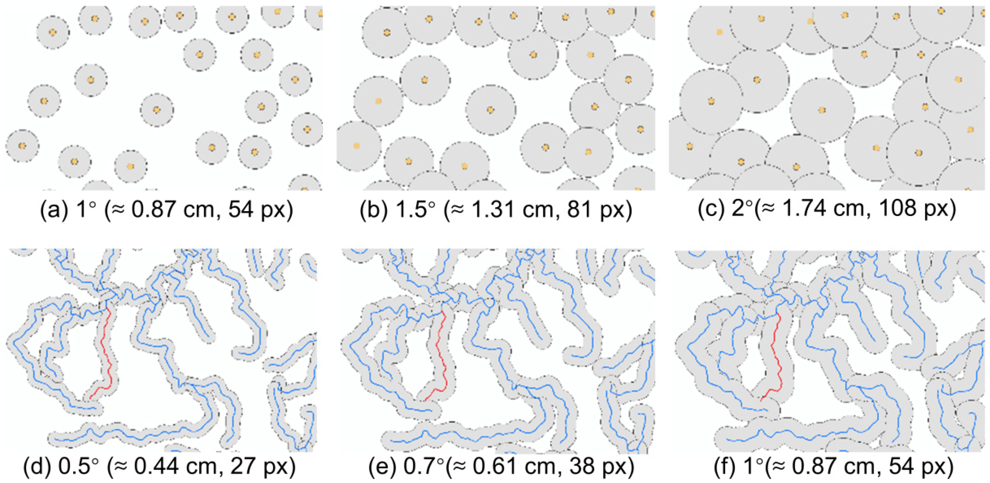
| Point | 200, 600, 1000 | 1° (≈0.87 cm, 54 px) 1.5° (≈1.31 cm, 81 px) 2° (≈1.74 cm, 108 px) |
| Polyline | 200, 600, 1000 | 0.5° (≈0.44 cm, 27 px) 0.7° (≈0.61 cm, 38 px) 1° (≈0.87 cm, 54 px) |
| Polygon | 200, 600, 1000 | Not applicable |
| Buffer Size | ||||
|---|---|---|---|---|
| Dwell Time | 1° | 1.5° | 2° | Avg. by Dwell Time |
| 200 ms | 3.97 (4.97) | 2.81 (3.47) | 2.62 (2.57) | 3.11 (3.80) |
| 600 ms | 3.29 (3.51) | 2.71 (2.90) | 2.74 (2.71) | 2.91 (3.06) |
| 1000 ms | 3.80 (3.22) | 3.53 (3.00) | 3.46 (3.34) | 3.60 (3.19) |
| Avg. by size | 3.69 (3.97) | 3.02 (3.15) | 2.94 (2.91) | |
| Buffer Size | ||||
|---|---|---|---|---|
| Dwell Time | 1° | 1.5° | 2° | Avg. by Dwell Time |
| 200 ms | 0.51 (0.17) | 0.50 (0.15) | 0.41 (0.11) | 0.47 (0.15) |
| 600 ms | 0.88 (0.13) | 0.88 (0.12) | 0.79 (0.16) | 0.85 (0.15) |
| 1000 ms | 0.97 (0.06) | 0.93 (0.14) | 0.90 (0.13) | 0.93 (0.12) |
| Avg. by size | 0.79 (0.24) | 0.77 (0.24) | 0.70 (0.22) | |
| Buffer Size | ||||
|---|---|---|---|---|
| Dwell Time | 0.5° | 0.7° | 1° | Avg. by Dwell Time |
| 200 ms | 4.03 (5.21) | 3.02 (3.40) | 2.97 (3.69) | 3.34 (4.17) |
| 600 ms | 3.80 (4.03) | 3.24 (3.03) | 2.74 (2.52) | 3.26 (3.24) |
| 1000 ms | 5.18 (5.60) | 4.35 (5.02) | 3.76 (3.48) | 4.43 (4.77) |
| Avg. by size | 4.33 (5.03) | 3.54 (3.92) | 3.16 (3.30) | |
| Buffer Size | ||||
|---|---|---|---|---|
| Dwell Time | 0.5° | 0.7° | 1° | Avg. by Dwell Time |
| 200 ms | 0.56 (0.18) | 0.49 (0.14) | 0.45 (0.14) | 0.50 (0.16) |
| 600 ms | 0.89 (0.13) | 0.83 (0.13) | 0.82 (0.13) | 0.85 (0.13) |
| 1000 ms | 0.94 (0.10) | 0.90 (0.13) | 0.89 (0.14) | 0.91 (0.13) |
| Avg. by size | 0.80 (0.22) | 0.74 (0.22) | 0.72 (0.24) | |
Publisher’s Note: MDPI stays neutral with regard to jurisdictional claims in published maps and institutional affiliations. |
© 2022 by the authors. Licensee MDPI, Basel, Switzerland. This article is an open access article distributed under the terms and conditions of the Creative Commons Attribution (CC BY) license (https://creativecommons.org/licenses/by/4.0/).
Share and Cite
Liao, H.; Zhang, C.; Zhao, W.; Dong, W. Toward Gaze-Based Map Interactions: Determining the Dwell Time and Buffer Size for the Gaze-Based Selection of Map Features. ISPRS Int. J. Geo-Inf. 2022, 11, 127. https://doi.org/10.3390/ijgi11020127
Liao H, Zhang C, Zhao W, Dong W. Toward Gaze-Based Map Interactions: Determining the Dwell Time and Buffer Size for the Gaze-Based Selection of Map Features. ISPRS International Journal of Geo-Information. 2022; 11(2):127. https://doi.org/10.3390/ijgi11020127
Chicago/Turabian StyleLiao, Hua, Changbo Zhang, Wendi Zhao, and Weihua Dong. 2022. "Toward Gaze-Based Map Interactions: Determining the Dwell Time and Buffer Size for the Gaze-Based Selection of Map Features" ISPRS International Journal of Geo-Information 11, no. 2: 127. https://doi.org/10.3390/ijgi11020127
APA StyleLiao, H., Zhang, C., Zhao, W., & Dong, W. (2022). Toward Gaze-Based Map Interactions: Determining the Dwell Time and Buffer Size for the Gaze-Based Selection of Map Features. ISPRS International Journal of Geo-Information, 11(2), 127. https://doi.org/10.3390/ijgi11020127