Possibilities for Assessment and Geovisualization of Spatial and Temporal Water Quality Data Using a WebGIS Application

Abstract

The provision of webGIS-based water quality data services has become a priority area for both the public and administrative sectors in the context of the pandemic emergency associated with the global spread of COVID-19. Current geographic, monitoring and decision supporting systems, typically based on web-based geospatial information, greatly facilitate the sharing of spatial and temporal data from environmental databases and real-time analyses. In the present study, different water quality indices are determined, compared and geovisualized, during which the changes in the quality of the shallow groundwater resources of a settlement are examined in the period (2011–2019) in an eastern Hungarian settlement. Another objective of the research is to determine three water quality indices (Water Quality Index, CCME Water Quality Index, Contamination degree) and categorize water samples based on the same input spatial and temporal data using self-developed freely available geovisualization tools. Groundwater quality was assessed by using different water quality indices. Significant pollution of the groundwater in the time period before the installation of a sewage network was shown. Regarding water quality, significant positive changes were shown based on all three water quality indices in the years after installing a sewage network (2015–2019). The presence of pollution apart from the positive changes suggests that the purification processes will last for a long time.

1. Introduction

The deterioration of groundwater quality is a global problem, making it a hot issue of environmental research [1]. International studies show that communal sewage is one of the most significant sources of pollution in addition to industrial and agricultural activities, the treatment and purification of which is often unresolved for developed and developing countries [2,3,4,5,6]. Several studies specified that the lack of sewage treatment systems in rural areas causes sewage to enter groundwater, resulting in a severe degradation in groundwater quality in these areas [7,8,9,10]. Having reviewed the international literature, we found that although publications have been published regarding the environmental problems caused by sewage generated in settlements, a comprehensive investigation that would present the water quality before and after the construction of the sewerage network covering an entire town has not yet been carried out. In addition, knowledge of the baseline condition is necessary to assess the water quality changes, but most municipalities do not have such a settlement-wide spatial and temporal water quality data or geodatabase thus making comparative analysis impossible. One of the aims of our study is to fill this scientific gap [11].

A number of methodological approaches have been taken to categorize groundwater between good and poor quality [12,13]. As water quality status can be described by a number of physical, chemical and biological parameters, large amounts of data make evaluation and comparison increasingly difficult [14]. To solve this problem, Horton (1965) proposed the introduction of the first water quality index based on 10 important water chemical parameters [15]. The most important advantage of the various pollution indices is the pooling of chemical, physical and biological parameters into a single number, which makes information on water quality comprehensible to the public and policymakers as well [16,17].

The Water Quality Index (WQI), developed by Brown et al. (1970) based on weighted averaging, has been amended several times in recent decades [18]. Based on the WQI, the US National Sanitation Foundation Water Quality Index (NSFWQI) and the Canadian Water Quality Index (Canadian Council of Ministers of the Environment (CCME)) were created [19].

Thematic maps, based on water quality indices, give a comprehensive picture of the environmental problem and are easy to understand for people outside the scientific field [20]. Thus, the use of water quality indices in the description of the quality of both surface water and groundwater has become standard practice [21,22,23,24]. In the following decades, a number of methods were developed to aggregate monitoring data into a single water quality indicator [25,26,27,28,29] and to visualize water quality indices in Geographical Information Systems (GIS) [30,31,32].

In the epidemiological emergency of the COVID-19 pandemic, the provision of webGIS-based data services on water quality has become a priority area for both the state and public administration sectors. Currently, geographical, monitoring and decision support systems, typically based on web-based geoinformatic technology, greatly help to share and analyze spatial and temporal data of environmental databases in real time. The publication of geographic environmental data on the web is largely shifted to infocommunication platforms; therefore, criteria such as up-to-dateness, platform independence or an easy-to-use and accessible "map-based" communication interface must be met. Since the "geoinformatic revolution" named by Schütze in 2007, webGIS development tools and frameworks have unwittingly set out a development direction in the sharing and geovisualization of geographic information [33]. In parallel with the spread of web-based spatial information systems, the environment in which users interpret and handle spatial data has also changed. In the age of digitalization, the need for information associated with a geographic location to be communicated using geovisualization tools [34,35,36,37,38,39] emerged. The range of users has been further expanded, which has been supplemented by civil users after professional data providers supporting industrial-research use. The possibilities of publishing spatial data on the web have been greatly facilitated by the fact that the best-known map providers (Google Maps, OSM, Yahoo! Maps, Bing Maps, MapQuest, etc.) provide a custom tool system (e.g. Leaflet, OSM, Google Maps API, Azure Maps API) free of charge to display the data [40,41,42,43]. As digitalization accelerated, the ability to navigate in the digital space and on the digital map also became important in the information society, which were gradually included among digital competences, confirmed by numerous multidisciplinary research projects [44,45,46,47,48]. Of course, the geovisualization procedures found in scientific publications are not limited to spatial data or databases alone, as these techniques aim to develop visualization techniques via the use of maps, enabling them to effectively serve different disciplines involving a number of other data sources [49,50,51,52,53].

The novelty of our study is based, among other things, on the fact that although the use of various web-based geovisualization tools is widespread in earth sciences, the geospatial processing and complex online representation of municipal environmental data has not been the focus of research to date. Furthermore, we aimed to answer the question as to whether the web publication of the spatial data generated by the developed tool could provide the end-user with additional information about the water quality status of the study area by using his/her own cognitive perception.

In the present study, with help of a WebGIS tool, three water quality indices (Water Quality Index, CCME Water Quality Index, Contamination degree) were determined, compared and geovisualized, in the course of which changes in the quality of the groundwater resources of a settlement in eastern Hungary are examined in the studied period (2011–2019) after the construction of a sewerage network in 2014. Based on the above, our purpose is to publish and demonstrate the spatial visualization and processing of temporal environmental data of a Hungarian settlement, and also highlight the power of geo-visualization.

The specific objectives of the study were the following:

• To develop an analytical web tool to determine and geovisualize water quality indices,
• To map water quality and the degree of contamination across the settlement by using exported and calculated water quality data,
• To assess the spatial and temporal water quality changes for the period 2011–2019,
• To determine how different indices, categorize water samples based on the same input data.

2. Materials and Methods

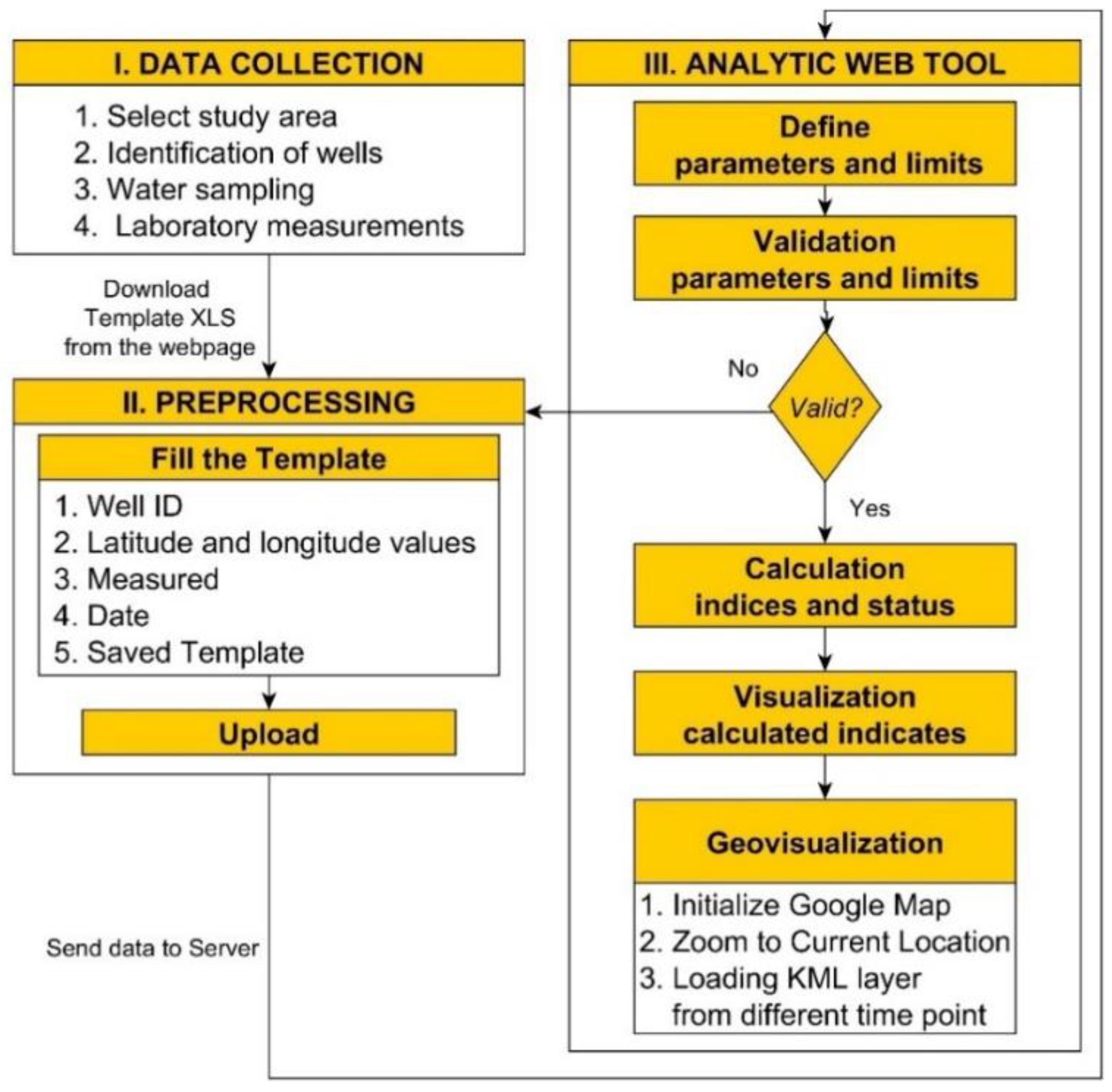
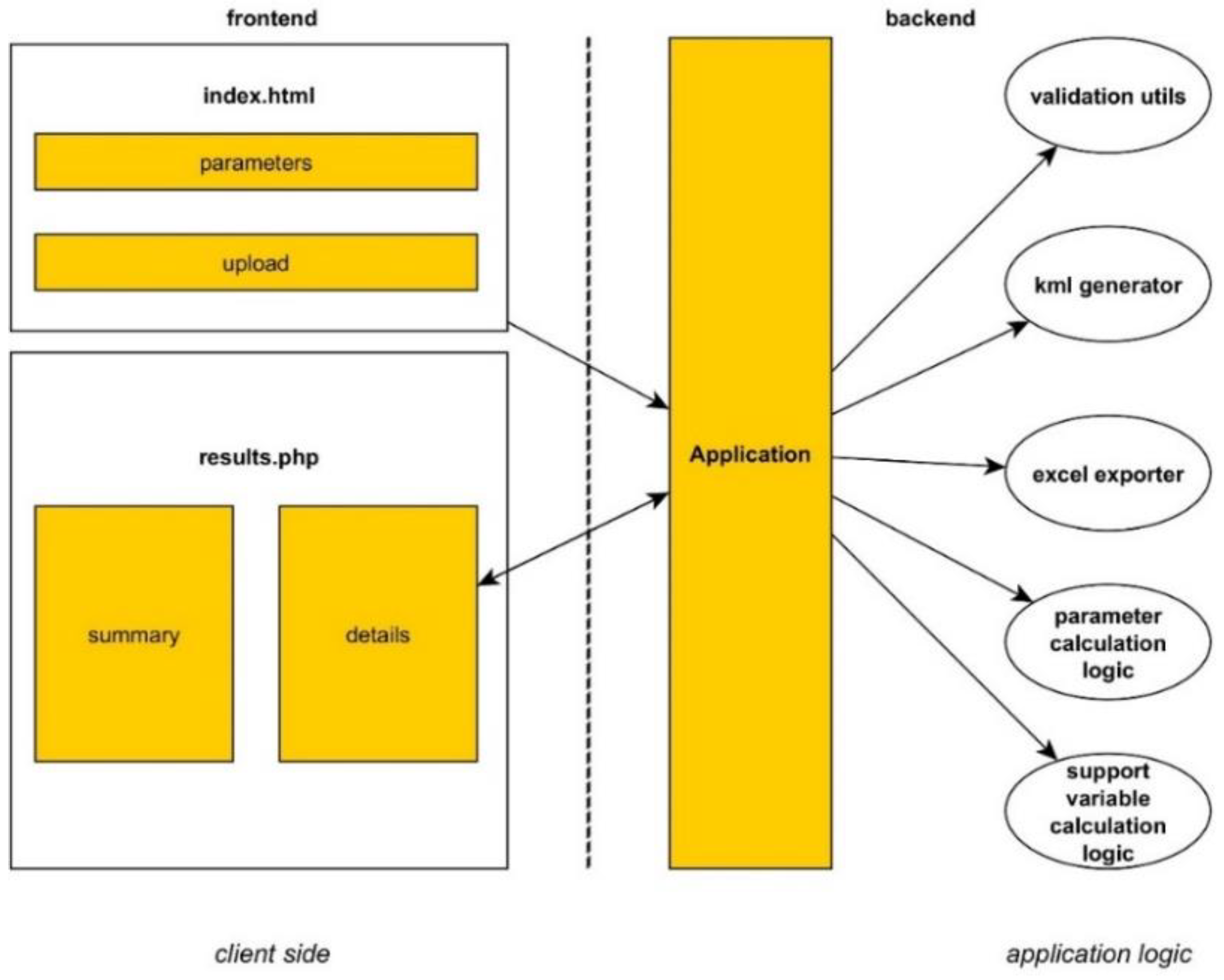
2.1. Development of Geovisualization Tool

The geovisualization tool was developed using different technologies and programming languages. The geovisualization of the webmap and spatial data was implemented using Google Maps application programming interface (API) v3, Keyhole Markup Language (KML) and Chart.js tools [54,55,56]. The determination of water quality indices was performed by a Javascript code by utilizing the formulas described in the previous section. A filled-up Excel template should be uploaded to the index page of the website so that the determination and geovisualization can be implemented (Figure 1). In order to create the portal, the BootStrap front-end framework created by the developer of Twitter and the interactive interface of Sufee Admin were used [57,58].

The code base was implemented following a procedural (imperative) programming paradigm. The server side part of the web application was developed using PHP [59,60]. The PHP language was chosen because it is a simple and widely used scripting language, easy to install locally on the server and capable of generating views using the PHP template. On the server side, the "app" component controls the execution, and requests are submitted into this app as well. In addition, the corresponding application logic is implemented here using collections of helper functions outsourced according to the target functionality (Figure 2). The view that generates the response is also defined here. The implementation is done using the template-generating capabilities of the PHP language. The basic structure of the HTML page is defined in the template, and the alternative control structure of the PHP language is used to dynamically generate the parts depending on the variable data volume and values. Afterwards, the server sends back to the client page the corresponding HTML page displayed to the user. The calculations are performed after the input data is received and the results are stored on the server in the user session. In this way, it is not necessary to perform the calculation tasks (export, view change) again for each request.

Basic validation is performed on the data received from the user side (e.g., whether a given field has a value, whether the value is within a given range, etc.). This kind of validation of incoming data allows us to prevent invalid data reaching calculation algorithms that would likely cause errors on the server side. In case of an error, the user is notified about the result in the form of an error message on the interface [61].

2.2. Determination and Evaluation of Indices

Eight parameters (pH, EC, NH₄⁺, NO₂⁻, NO₃⁻, PO₄³⁻, COD, Na⁺) were used to calculate the Water Quality Index (WQI), Canadian Council of Ministers of the Environment Water Quality Index (CCME WQI) and Contamination degree (Cd).

Water Quality Index (WQI)

Calculation of the WQI was carried out following the ‘weighted arithmetic index method’ using the equation [18]:

$$\mathit{W}\mathit{Q}\mathit{I}=\sum {\mathit{Q}}_{\mathit{n}}{\mathit{W}}_{\mathit{n}}/\sum {\mathit{W}}_{\mathit{n}}$$

where Q_n is the quality rating of the n^th water quality parameter, W_n is the unit weight of the nth water quality parameter. The quality rating Q_n is calculated using the equation:

$${\mathit{Q}}_{\mathit{n}}=\mathbf{100}\left[\left({\mathit{V}}_{\mathit{n}}-{\mathit{V}}_{\mathit{i}}\right)/\left({\mathit{V}}_{\mathit{s}}-{\mathit{V}}_{\mathit{i}}\right)\right]$$

where V_n is the actual amount of the n^th parameter present, V_i is the ideal value of the parameter [V_i = 0, except for pH (V_i = 7)] and V_s is the standard permissible value for the nth water quality parameter. The unit weight (W_n) is calculated using the formula:

$${\mathit{W}}_{\mathit{n}}=\mathit{k}/{\mathit{V}}_{\mathit{s}}$$

where k is the constant of proportionality and is calculated using the equation:

$$\mathit{k}=\left[\mathbf{1}/\sum \mathbf{1}/{\mathit{V}}_{\mathit{s}}=\mathbf{1},\mathbf{2},\dots ,\mathit{n}\right]$$

CCME Water Quality Index (CCME_wqi)

This is a rating system developed by the Canadian Council of Ministers of the Environment in 2001 [19]. The ranking system is based on a combination of three factors:

F1: Number of parameters tested that exceed the contamination limit (Scope).

$$\mathit{F}\mathbf{1}=\left(\frac{\mathit{n}\mathit{u}\mathit{m}\mathit{b}\mathit{e}\mathit{r}\mathit{o}\mathit{f}\mathit{f}\mathit{a}\mathit{i}\mathit{l}\mathit{e}\mathit{d}\mathit{p}\mathit{a}\mathit{r}\mathit{a}\mathit{m}\mathit{e}\mathit{t}\mathit{e}\mathit{r}\mathit{s}}{\mathit{t}\mathit{o}\mathit{t}\mathit{a}\mathit{l}\mathit{n}\mathit{u}\mathit{m}\mathit{b}\mathit{e}\mathit{r}\mathit{o}\mathit{f}\mathit{p}\mathit{a}\mathit{r}\mathit{a}\mathit{m}\mathit{e}\mathit{t}\mathit{e}\mathit{r}\mathit{s}}\right)\times \mathbf{100}$$

F2: The percentage of failed tests (Frequency).

$$\mathit{F}\mathbf{2}=\left(\frac{\mathit{N}\mathit{u}\mathit{m}\mathit{b}\mathit{e}\mathit{r}\mathit{o}\mathit{f}\mathit{f}\mathit{a}\mathit{i}\mathit{l}\mathit{e}\mathit{d}\mathit{t}\mathit{e}\mathit{s}\mathit{t}\mathit{s}}{\mathit{t}\mathit{o}\mathit{t}\mathit{a}\mathit{l}\mathit{n}\mathit{u}\mathit{m}\mathit{b}\mathit{e}\mathit{r}\mathit{o}\mathit{f}\mathit{t}\mathit{e}\mathit{s}\mathit{t}\mathit{s}}\right)\times \mathbf{100}$$

F3: The amount by which failed test values do not meet their objectives (Amplitude). Factor 3 can be calculated in three steps:

$$\mathit{e}\mathit{x}\mathit{c}\mathit{u}\mathit{r}\mathit{s}\mathit{i}\mathit{o}{\mathit{n}}_{\mathit{i}}=\left(\frac{\mathit{f}\mathit{a}\mathit{i}\mathit{l}\mathit{e}\mathit{d} \mathit{t}\mathit{e}\mathit{s}\mathit{t} \mathit{v}\mathit{a}\mathit{l}\mathit{u}{\mathit{e}}_{\mathit{i}}}{\mathit{O}\mathit{b}\mathit{j}\mathit{e}\mathit{c}\mathit{t}\mathit{i}\mathit{v}{\mathit{e}}_{\mathit{j}}}\right)-\mathbf{1}$$

$$\mathit{n}\mathit{s}\mathit{e}=\frac{{{\displaystyle \sum }}_{\mathit{i}=\mathbf{1}}^{\mathit{n}}\mathit{e}\mathit{x}\mathit{c}\mathit{u}\mathit{r}\mathit{s}\mathit{i}\mathit{o}{\mathit{n}}_{\mathit{i}}}{\mathbf{0.01}\mathit{n}\mathit{s}\mathit{e}+\mathbf{0.01}}$$

$$\mathit{F}3=\frac{\mathit{n}\mathit{s}\mathit{e}}{\mathbf{0.1}\mathit{n}\mathit{s}\mathit{e}+\mathbf{0.01}}$$

After calculating all the three factors, the WQI can be determined by the following equation:

$$\mathit{C}\mathit{C}\mathit{M}\mathit{E}\mathit{W}\mathit{Q}\mathit{I}=\mathbf{100}-\left(\frac{\sqrt{\mathit{F}{\mathbf{1}}^{\mathbf{2}}}+\mathit{F}{\mathbf{2}}^{\mathbf{2}}+\mathit{F}{\mathbf{3}}^{\mathbf{2}}}{\mathbf{1.732}}\right)$$

The factor value of 1.732 is introduced to a scale index ranging from 0 to 100, where 0 is the “worst”, and 100 is the “best” WQI value.

Contamination degree (Cd)

The calculation of the contamination degree, Cd, is made separately for each sample of water analyzed, as a sum of the contamination factors of individual components exceeding the upper permissible value. Hence, the contamination index summarizes the combined effects of several quality parameters considered harmful to household water.

The scheme for the calculation of Cd is the following [29]:

$${\mathbf{C}}_{\mathbf{d}}={\displaystyle \sum }_{\mathbf{i}=\mathbf{1}}^{\mathbf{n}}{\mathbf{C}}_{\mathbf{f}\mathbf{i}}$$

where

$${\mathbf{C}}_{\mathbf{f}\mathbf{i}}=\frac{{\mathbf{C}}_{\mathbf{A}\mathbf{i}}}{{\mathbf{C}}_{\mathbf{N}\mathbf{i}}}-\mathbf{1}$$

C_fi= contamination factor for the i–th component,

C_Ai= analytical value of the i–th component,

C_Ni= upper permissible concentration of the i–th component (N denotes the “normative” value).

The elements and ionic species with analytical values below the upper permissible concentration values are not taken into consideration.

The evaluation of the WQS, CCME WQS and Cd statuses are shown in

Table 1. WQI range, WQS status, CCME WQI range, CCME WQS status, Cd range, Cd status and possible use of the water sample.

Rank	WQI	Water Quality Status (WQS)	CCME WQI	CCME Water Quality Status (WQS)	Cd	Cd Status	Possible Use
R1	0–25	Excellent water quality	95–100	Excellent	0	Excellent	Drinking, irrigation and industrial
R2	26–50	Good water quality	80–94	Good	<1	Low	Irrigation and industrial
R3	51–75	Poor water quality	65–79	Fair	3–1	Medium	Irrigation and industrial
R4	76–100	Very poor water quality	45-64	Marginal	6–3	High	Irrigation
R5	Above 100	Unsuitable for any use	0–44	Poor	>6	Very High	Proper treatment required before use

.

2.3. Description of Study Area

Significant progress was made in the collection and purification of municipal sewage in Hungary in the last decade. The difference in the proportion of dwellings connected to the water network and the sewerage network decreased from 31.5% in 2004 to 13.3% in 2018; thus, the secondary utility difference is expected to fall below 10% within a few years [62]. As a result of the investments made, the amount of municipal sewage entering the groundwater system is significantly reduced, the impact of which extends over the entire municipal environment. In order to be able to accurately determine the extent, intensity and duration of these changes, it is essential to survey the pre-investment conditions apart from continuous groundwater monitoring.

Báránd settlement is located in the eastern part of the Great Hungarian Plain (Figure 3). It has a population of 2611 [62]. Construction of the sewerage network in the settlement was completed in 2014. By 2017, more than 95% of households had joined the network. According to our calculations, 30–40% of the domestic wastewater generated (appr. 120,000 m³ each year) could have seeped into the soil and groundwater over the past few decades. This significant pollution discharge has caused heavy contamination in the settlement. Because of this contamination, the wells are monitored every year to detect potentially contaminated areas [63].

2.4. Water Sampling and Laboratory Measurements

In our research, 15 groundwater wells were investigated in the period 2011–2019. Water samples were collected from the upper 1 m water column of each well. The pH and EC were measured with a WTW 315i handheld meter and the NH₄⁺, NO₂⁻, NO₃⁻, PO₄³⁻ content of the collected water samples were determined using appropriate procedures according to the Hungarian Standards [64,65,66]. The Chemical Oxygen Demand COD was determined using the KMnO₄ method, and Na⁺ was determined by using a Perkin Elmer 3110 AAS.

2.5. Statistical Analysis

The software IBM SPSS 26 was used to perform statistical processing of the data series and to represent the results. The normality of the series was examined using the Shapiro–Wilk test. In addition to the calculation of the basic statistical values, mean, lower and upper quartile, mode, median and standard deviation boxplot diagrams were used for plotting the interquartile range, median, highest and lowest values.

Based on our hypothesis, the establishment of the sewerage system affects the quality of the groundwater; therefore, it was expected that the water quality would improve significantly after the construction of the sewerage network. To test our hypothesis, statistical tests were performed. Since, on the basis of the Shapiro–Wilk test, the data sets do not show normal distribution, evaluations of any positive or negative changes in the data sets are performed using the nonparametric Wilcoxon signed-ranks test [67]. Wilcoxon signed-ranks test is widely used to determine whether there is an average difference between two paired data, when the normality assumption is doubtful. If the value of Asymp. Sig. (2-tailed) is smaller than <0.05, then Ha is accepted. Conversely, if the value of Asymp. Sig. (2-tailed) is greater than >0.05, then Ha is rejected.

3. Results

3.1. Description of Geovisualization Tool

A geovisualization web tool was developed which can be used to determine and geovisualize groundwater quality based on the input spatial and temporal water quality data. The work process can be divided into three main parts. During the first part, the study area should be selected, the wells located in the area should be identified and their geographic positions should be recorded. During the second part, following the completion of a template, the document can be uploaded to the webserver where, after the validation of the given parameters is performed, water quality and degree of contamination indices of temporal data are determined and geovisualized. The validation of parameters and limit values includes quality assurance methods which make it easier to identify and correct the errors of the input data – whether it was recorded in the field or added later as measured laboratory data. This means that during the determination of water quality, the user will not receive a misleading result because of the incorrectly recorded parameters, thereby improving the accuracy of the water quality determination process. If any of the parameters provided by the user are incorrect, the server sends a message to the users informing them about the incorrect parameters or limit values which should be corrected before upload and analysis [61].

Native JavaScript has been used to manage user interactions. The user interface is supported by components developed in the Bootstrap CSS framework, which provides the most intuitive and comfortable environment for the user in terms of "user experience". On the home page, the user has the possibility to specify the exact location of the Microsoft Excel file on his/her computer containing the parameters on which the calculations are based. The default values for other parameters relevant to the processing are also provided here and can be modified as required.

The results are displayed on a new page after the appropriate calculations have been made. The user can view the calculation results in a summary view or see details in both tabular and geovisualised forms (Figure 4). Data visualization and geovisualization for faster and more efficient cognitive interpretation and easier overview are implemented using Google Maps map and Chart.js chart drawing library. In terms of use, the input data are obtained from a standard Microsoft Excel file and the calculation results can be exported from the application in the same format (Figure 4).

The spatial data of the investigated wells are converted into KML format. This provides a standard format that can be used in external systems. This is achieved by uploading a KML template, based on an own designed logic. Additionally, a customized JavaScript-based KML parser was implemented for the generated format, which is the basis for the visualization on the map. Geolocation on the map is performed using the Google Maps JavaScript API. These KML management tools have been developed in an application-independent and reusable way.

The geovisualization of water quality indices and water quality statuses are provided by the interactive user interface which represent the ratio of the values of each water quality indices and the ratio of their potential usage based on the water quality of groundwater wells. The data to be visualized on the webmap are represented by KML layer. The KML layer contains the results of indices determined based on the groundwater quality parameters of the uploaded wells, where information bubbles near the placemark show the investigated wells based on the degree of contamination, using unique symbols (Figure 5 and Figure 6).

The main advantages of using 2D geo- and data visualization with a web application are that the geospatial pre-processing (data structure creation, database management, styling, layer management, water quality index definition, analysis) and publication of time series spatially referenced environmental data imported into the system can be done in one interface; therefore, no additional platform or software environment is required for post-processing. An additional advantage is that after exporting the KML, it can be interpreted by many other geographic information systems apart from Google Earth and Google Maps, and can perform conversions between systems, allowing users to visualize complex spatial analyses without programming knowledge. As users do not need their own server to share the data on the web, the results are available to anyone after processing. However, due to the upload limit, visualization of larger databases is not enabled in the current version of this application. Another drawback in terms of geovisualization is that the size of the input data reduces the speed of data loading as well.

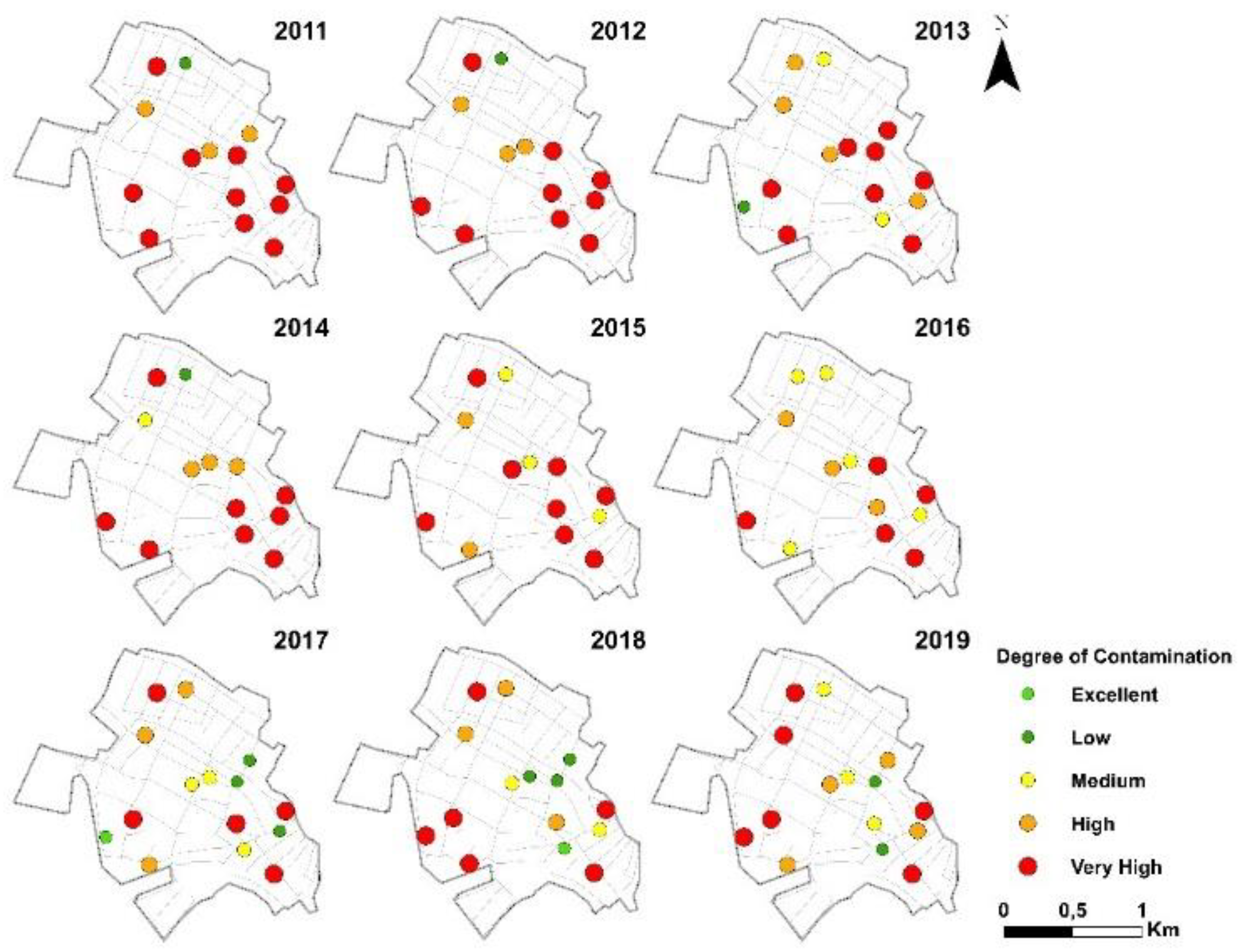
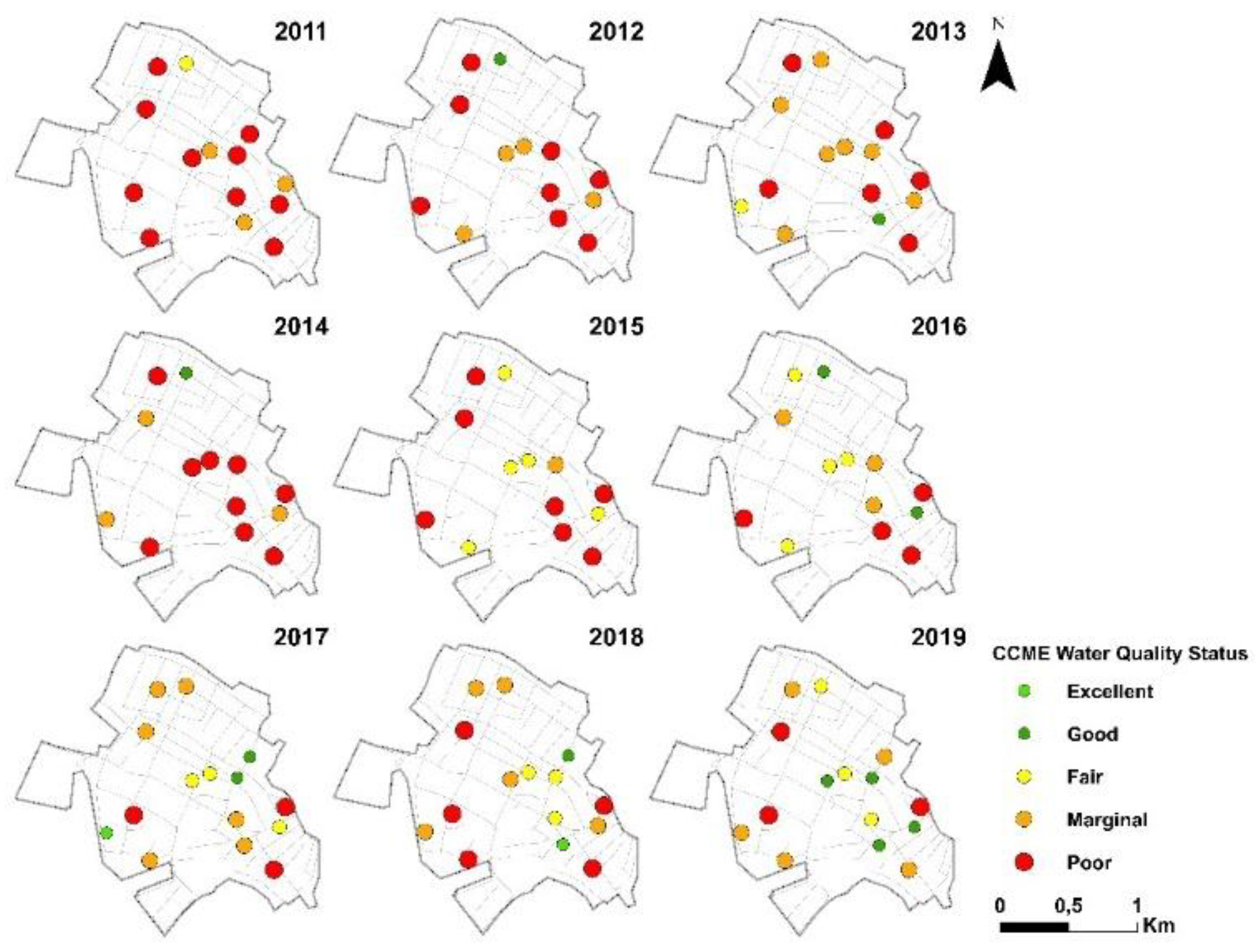
3.2. Spatial and Temporal Distribution of Groundwater Quality

In order to explore and analyze the spatial and temporal distribution of exported water quality data, the values for each well were also plotted on thematic maps. The results were performed with ArcGIS 10.4.1 software. After categorising the water quality of the wells, pollution maps of the settlement considering the different indices and sampling years were prepared. Regarding the spatial changes of the degree of contamination, it was found that in the period before the establishment of the sewerage network, the central and south-eastern areas of the settlement can be regarded the most polluted, where the majority of the wells were classified category 5 regarding water quality in the case of all three indices (Figure 7, Figure 8, Figure 9).

Following the transition period of 2015–2016, the proportion of wells marked with a red color code decreased spectacularly during the period of 2017–2019. In the central areas of the settlement, the degree of contamination decreased by 1–2 categories for almost all wells. For all three indices, the water quality status "Good" appeared in the central and southern areas of the settlement in the case of Cd and CCMEwqi (Figure 7, Figure 8, Figure 9).

Based on the changes revealed, it can be stated that the purification processes in the area have begun, but our results show that pollutants entering the environment remain in the system for a long time. Further long-term groundwater monitoring is necessary to track changes of the contamination in both time and space.

3.3. Assesment of Spatial and Temporal Changes of Water Quality

The index values (WQI) determined on the basis of input data are plotted on boxplot diagrams by year, indicating the category related to the value. The index values were then classified into 5 pollution categories (WQS), where the first was the best and the fifth was the worst quality (Figure 10,

Table 2. Descriptive statistics of index values.

		WQI					Cd					CCMEWQI
Date	N	Min.	Max.	Mean	Q 25	Q 75	Min.	Max.	Mean	Q 25	Q 75	Min.	Max.	Mean	Q 25	Q 75
2011	14	46.1	182.7	113	64.9	143	0.5	22.8	11.3	5.3	15.9	25.7	79.3	41	33.3	47.3
2012	13	40.2	223.6	129.5	76.5	157.2	0.2	19.3	9.1	4.8	13.9	28.2	89.7	43	29.1	53
2013	15	80.2	306.7	172.8	96.2	266.2	0.2	15	7	3.6	9.9	19.8	87.6	48.1	28.5	63.5
2014	13	39.8	205.2	118.6	87.8	150.9	0.5	27	10	5.1	14.6	23	89.2	42.9	26.2	50.2
2015	13	45.1	560.4	209.9	93.3	257.3	2.0	22.5	10.8	2.8	16.4	17.8	76.5	44.9	27.6	66.9
2016	13	45	449.3	136.2	69.8	169.8	1.4	15.9	6.9	2.2	13.2	28.7	86.7	58.8	39.5	75.3
2017	15	25.2	282.5	90.3	37	116.6	0	18.7	4.6	0.6	6.7	33.4	100	62	46	79.1
2018	15	49.5	403.6	124.1	67.3	143	0	11.8	5	0.7	8.9	34.7	100	58.1	41.7	69.1
2019	15	33.1	367.9	105.8	50.7	112.1	0.5	13.8	5.7	2.5	8.9	32.9	89.2	60.6	45.2	80.2

).

In the case of Brown’s WQI, it can be clearly seen that in the years before the establishment of the sewerage network (2011–2014) the majority of wells were classified "Unsuitable" or "Very poor" and after a two-year transition period (2017–2019), both the upper and lower quartiles showed a clear decrease (Figure 10). According to WQS, the number of category 5 (Unsuitable) wells decreased by 40% in the years following the establishment of the sewerage network (Figure 10,

Table 3. Number of the monitoring wells with different indices in the investigated periods (2011–2019).

		WQS					Cds					CCMEWQS
Date	N	R1	R2	R3	R4	R5	R1	R2	R3	R4	R5	R1	R2	R3	R4	R5
2011	14	0	1	3	0	10	0	1	0	3	10	0	0	1	3	10
2012	13	0	1	2	1	9	0	1	0	3	9	0	1	0	4	8
2013	15	0	0	0	4	11	0	1	2	4	8	0	1	1	7	6
2014	13	0	2	0	4	7	0	1	1	3	8	0	1	0	3	9
2015	13	0	1	1	2	9	0	0	3	2	8	0	0	5	1	7
2016	13	0	1	2	4	6	0	0	5	3	5	0	2	4	3	4
2017	15	1	3	4	2	5	1	3	3	3	5	1	2	3	6	3
2018	15	0	1	4	4	6	1	3	2	3	6	1	1	3	5	5
2019	15	0	4	2	3	6	0	2	3	4	6	0	4	3	5	3

). While the median values ranged within the "Unsuitable" category until 2015, they were in the "Poor" or "Very Poor" categories from 2016. The positive changes are also illustrated by the fact that five years after the establishment of the sewerage network, 40% of the wells were in the categories 2 and 3 (Good, Poor), while in the years before the establishment of the sewerage network this proportion was around 0–26% (Figure 10, Table 3).

Purification processes can be detected based on the Cd index as well. In the period before the establishment of the sewerage network, both the lower and upper quartiles were in the worst "Very high" category. However, after establishment of the sewerage network, the lower quartiles shifted into the category "Medium" or "High". The values of the upper quartiles also decreased significantly, from 13.58 before the establishment of the sewerage network to 8.27. The average value of the pre-sewerage period (8.61) decreased to 5.29. In the case of WQS, the number of wells in the most polluted category typically decreased by 40% (Figure 10, Table 2).

Considering CCME WQI, higher index values mean better water quality. The average value of 43.86 in the pre-sewerage period increased by nearly 30% to 59.56 in the period between 2016 and 2019. The lower quartile rose from 29.3 to 41.9, while the upper quartile rose from 53 to 77.1 in the post-sewerage period. Thus, while the values of the upper quartile were in the "Marginal" category in the pre-sewerage period, they were in the one higher "Fair" category each year from 2016 onwards after the sewerage network was established. The number of wells in the worst category showed the most significant decrease in the case of this index. In the post-sewerage years, it typically decreased by 30–50% compared to the pre-sewerage years (Figure 10).

Of course, the effects of sewerage on water quality do not occur immediately, and there is also a natural change in each year. Therefore, in order to better illustrate the effects of sewerage on index values by eliminating fluctuations in each year, the data series was broken down into 3 periods: 1/ the period before the establishment of the sewerage network between 2011 and 2014; 2/ the transition period of 2015–2016; and 3/ the period after the establishment of the sewerage network between 2017 and 2019 (Figure 11). Although positive changes can be seen during the two-year transition period, these values are still more closely related to the data series of the pre-sewerage period. Data for the period 2017–2019 are clearly separate from the data for the pre-sewerage period (Figure 11). The positive changes are supported by further statistical analyses as well. Studying the pre-sewerage (2011–2014) and post-sewerage (2017–2019) data series using Wilcoxon’s signed-ranks test significant differences were shown for all three indices, which is clearly explained by the effects of the sewerage network (Figure 11). The strongest significance (p=0.001) was found in the case of the CCCMEwqi, where the Z value was -3.279. For Cd and WQI nearly identical values were obtained, which significantly indicate the positive effects of sewerage albeit to a lesser extent (

Table 4. Results of Wilcoxon signed-ranks test (a. Wilcoxon signed-ranks test; b. Based on negative ranks; c. Based on positive ranks).

	CCME_after-CCME_before	WQI_after-WQI_before	Cd_after-Cd_before
Z	–3.279b	–2.726c	–2.636c
Asymp. Sig. (2-tailed)	0.001	0.006	0.008

).

4. Discussion

According to the aims given by [35], “geovisualization is both a process for leveraging the data resources to meet scientific and social needs and a research field that develops visual methods and tools to support a wide array of geospatial data applications. To support real-world knowledge construction and decision making, some of the most important challenges involve distributed geovisualization—that is, enabling geovisualization across software components, devices, people, and places.” This specific field has already become widely known in many fields of environmental science, as is proved by several scientific papers containing sections which also highlight the geovisualization aspects of their results [34,35,45,47].

The validity of our study has been supported by other case studies that focus on the design, development and analysis of user-centered, novel collaborative geovisualization tools [68,69,70]. Studies are consistent in that an easy-to-use graphical user interface, decision support based on spatial data and the integration of data into other platforms are essential for efficient geovisualization [69,70]. However, it should be underlined that while innovative geovisualization web applications published on the basis of current trends are supported by a wide range of standards, development tools and frameworks, the inclusion of the latest IT technologies (Big Data, Cloud, Artificial Intelligence) offers an interesting research challenge.

Based on the results of geovisualization, our study showed a high level of contamination of the groundwater resources of the settlement in the period without sewerage, which is in accordance with similar studies carried out in municipal environment [23,26,28]. Data from studies on groundwater quality change following the construction of the sewerage network showed positive changes in groundwater quality, similar to our own results [11]. At the same time, it is important to mention that literature on improved water quality after sewerage is limited, which is one of the reasons why our long-term monitoring results can be important additions to the literature and may draw widespread interest.

5. Conclusions

In the course of our research, changes in groundwater quality in a settlement after the establishment of a sewerage network were evaluated using three different water quality indices. Based on input data for the pre-sewerage (2011–2014), transitional (2015–2016) and post-sewerage (2017–2019) periods, significant positive changes for all three indices were found. For index values, both the lower and upper quartiles shifted towards better water quality. While in the pre-sewerage period the majority of wells were classified as highly contaminated, contaminated (Rank 4–5), in the post-sewerage period, the number of wells with low or medium contamination (Rank 2–3) increased significantly for all three indices.

Assessing the spatial changes of the contamination, it was found that the inner and south-eastern areas of the settlement were the most polluted in the period before the sewerage network was established. In the period following the establishment of the sewerage network, the degree of contamination in the inner areas of the settlement decreased by 1–2 categories in almost all wells. For all three indices, the water quality status "Good" (rank 2) appeared in the central and southern areas of the settlement. However, in addition to significant positive changes, the level of contamination remains high in many cases, which highlights that, although the purification processes have started, they will last for a long time to come. Further long-term groundwater monitoring is necessary to track the changes of contamination in both time and space.

The complexity of the term geovisualization closely reflects its interdisciplinary or multidisciplinary characteristics, since acquiring information by observing geovisualized spatial and temporal water quality data can support different cognitive processes. The key factor is demonstrated in the process of geovisualization, during which uploaded data of monitoring wells were transformed into a special form enhancing the co-evolvement of cognitive processes with WebGIS tool:

• The most important advantage of developed geovisualization tools is the visualized spatial environmental data, which makes valuable information understandable for both the public and decisionmakers.
• Revealing relationships between the investigated wells and the location became easier after geovisualization.
• Geovisualization facilitates the capturing of the spatial pattern of the distribution of different water quality indices at different times.
• The general cognitive perception of digital data is supported. The more parameters are used, a greater need can be identified for supporting the appropriate interpretation of the data.

References

1. Azzellino, A.; Colombo, L.; Lombi, S.; Marchesi, V.; Piana, A.; Andrea, M.; Alberti, L. Groundwater diffuse pollution in functional urban areas: The need to define anthropogenic diffuse pollution background levels. Sci. Total Environ. 2019, 656, 1207–1222. [Google Scholar] [CrossRef] [PubMed]
2. Jumma, A.J.; Mohd, E.T.; Noorazuan, M.H. Groundwater pollution and wastewater management in Derna City, Libya. Int. Environ. Res. J. 2012, 6, 50–54. [Google Scholar]
3. Ravikumar, P.; Somashekar, R.K. Assessment and modelling of groundwater quality data and evaluation of their corrosiveness and scaling potential using environmetric methods in Bangalore South Taluk, Karnataka state, India. Water Resour. 2012, 39, 446–473. [Google Scholar] [CrossRef]
4. Machiwal, D.; Jha, M.K. Identifying sources of groundwater contamination in a hard-rock aquifer system using multivariate statistical analyses and GIS-based geostatistical modeling techniques. J. Hydrol. Reg. Stud. 2015, 4, 80–110. [Google Scholar] [CrossRef] [Green Version]
5. Smoroń, S. Quality of shallow groundwater and manure effluents in a livestock farm. J. Water Land Dev. 2016, 29, 59–66. [Google Scholar] [CrossRef]
6. Adimalla, N.; Qian, H. Groundwater chemistry, distribution and potential health risk appraisal of nitrate enriched groundwater: A case study from the semi-urban region of South India. Ecotoxicol. Environ. Saf. 2020, 207, 111277. [Google Scholar] [CrossRef]
7. Backman, B.; Bodiš, D.; Lahermo, P.; Rapant, S.; Tarvainen, T. Application of a groundwater contamination index in Finland and Slovakia. Environ. Earth Sci. 1998, 36, 55–64. [Google Scholar] [CrossRef]
8. Rotaru, A.; Răileanu, P. Groundwater contamination from waste storage works. Environ. Eng. Manag. J. 2008, 7, 731–735. [Google Scholar] [CrossRef]
9. Devic, G.; Djordjevic, D.; Sakan, S. Natural and anthropogenic factors affecting the groundwater quality in Serbia. Sci. Total Environ. 2014, 468–469, 933–942. [Google Scholar] [CrossRef]
10. Nemčić-Jurec, J.; Singh, S.K.; Jazbec, A.; Gautam, S.K.; Kovač, I. Hydrochemical investigations of groundwater quality for drinking and irrigational purposes: Two case studies of Koprivnica-Križevci County (Croatia) and district Allahabad (India). Sustain. Water Resour. Manag. 2017, 5, 467–490. [Google Scholar] [CrossRef]
11. Khorasani, H.; Kerachian, R.; Aghayi, M.M.; Zahraie, B.; Zhu, Z. Assessment of the impacts of sewerage network on groundwater quantity and nitrate contamination: Case study of Tehran. In World Environmental and Water Resources Congress 2020: Groundwater, Sustainability, Hydro-Climate/Climate Change, and Environmental Engineering, Henderson, NV, USA, 17–21 May, 2020; American Society of Civil Engineers: Reston, VA, USA, 2020; pp. 53–66. [Google Scholar] [CrossRef]
12. Payne, S.M.; Woessner, W.W. An Aquifer Classification System and Geographical Information System-Based Analysis Tool for Watershed Managers in the Western U.S. J. Am. Water Resour. Assoc. (JAWRA) 2010, 46, 1003–1023. [Google Scholar] [CrossRef]
13. Lowe, M.; Wallace, J.; Kneedy, J.L. Ground-Water Recharge-Area and Water Quality-Classification Mapping for Cedar Valley, Southwestern Utah–Tools for Land-Use Planning. In Proceedings of the GSA Rocky Mountain 54th Annual Meeting, Denver, CO, USA, 7–9 May 2002. [Google Scholar]
14. Reisenhofer, E.; Adami, G.; Barbieri, P. Using chemical and physical parameters to define the quality of karstic freshwaters (Timavo River, North-eastern Italy): A chemometric approach. Water Res. 1998, 32, 1193–1203. [Google Scholar] [CrossRef]
15. Horton, R.K. An index number system for rating water quality. J. Water Pollut. Control Fed. 1965, 37, 300–306. [Google Scholar]
16. Ball, R.O.; Church, R.L. Water Quality Indexing and Scoring. J. Environ. Eng. Div. 1980, 106, 757–771. [Google Scholar] [CrossRef]
17. Bouslah, S.; Djemili, L.; Houichi, L. Water quality index assessment of Koudiat Medouar Reservoir, northeast Algeria using weighted arithmetic index method. J. Water Land Dev. 2017, 35, 221–228. [Google Scholar] [CrossRef]
18. Brown, R.M.; McClelland, N.I.; Deininger, R.A.; Tozer, R.G. A Water Quality Index: Do We Dare? Water Sew. Work. 1970, 117, 339–343. [Google Scholar]
19. Lumb, A.; Halliwell, D.; Sharma, T. Application of CCME Water Quality Index to Monitor Water Quality: A Case Study of the Mackenzie River Basin, Canada. Environ. Monit. Assess. 2006, 113, 411–429. [Google Scholar] [CrossRef]
20. Stigter, T.Y.; Ribeiro, L.; Dill, A.C. Application of a groundwater quality index as an assessment and communication tool in agro-environmental policies—Two Portuguese case studies. J. Hydrol. 2006, 327, 578–591. [Google Scholar] [CrossRef]
21. Liou, S.-M.; Lo, S.-L.; Wang, S.-H. A Generalized Water Quality Index for Taiwan. Environ. Monit. Assess. 2004, 96, 35–52. [Google Scholar] [CrossRef]
22. Bora, M.; Goswami, D.C. Water quality assessment in terms of water quality index (WQI): Case study of the Kolong River, Assam, India. Appl. Water Sci. 2017, 7, 3125–3135. [Google Scholar] [CrossRef] [Green Version]
23. Roba, C.; Balc, R.; Creta, F.; Andreica, D.; Padurean, A.; Pogacean, P.; Chertes, T.; Moldovan, F.; Mocan, B.; Rosu, C. Assessment of groundwater quality in NW of Romania and its suitability for drinking and agricultural purposes. Environ. Eng. Manag. J. 2021, 20, 435–447. [Google Scholar] [CrossRef]
24. Zessner, M. Monitoring, Modeling and Management of Water Quality. Water 2021, 13, 1523. [Google Scholar] [CrossRef]
25. Aljanabi, Z.Z.; Al-Obaidy, A.-H.M.J.; Hassan, F.M. A brief review of water quality indices and their applications. IOP Conf. Ser. Earth Environ. Sci. 2021, 779, 102088. [Google Scholar] [CrossRef]
26. Soltan, M.E. Evaluation Of Ground Water Quality In Dakhla Oasis (Egyptian Western Desert). Environ. Monit. Assess. 1999, 57, 157–168. [Google Scholar] [CrossRef]
27. Štambuk-Giljanović, N. Water quality evaluation by index in Dalmatia. Water Res. 1999, 33, 3423–3440. [Google Scholar] [CrossRef]
28. Pesce, S.F. Use of water quality indices to verify the impact of Córdoba City (Argentina) on Suquía River. Water Res. 2000, 34, 2915–2926. [Google Scholar] [CrossRef]
29. Rapant, S.; Vrana, K.; Bodis, D. Geochemical Atlas of Slovak Republic: Groundwater; Geofond: Bratislava, Slovakia, 1995; Volume 1. [Google Scholar]
30. Sha, J.; Li, X.; Zhang, M.; Wang, Z.-L. Comparison of Forecasting Models for Real-Time Monitoring of Water Quality Parameters Based on Hybrid Deep Learning Neural Networks. Water 2021, 13, 1547. [Google Scholar] [CrossRef]
31. Hajji, S.; Yahyaoui, N.; Bousnina, S.; Ben Brahim, F.; Allouche, N.; Faiedh, H.; Bouri, S.; Hachicha, W.; Aljuaid, A.M. Using a Mamdani Fuzzy Inference System Model (MFISM) for Ranking Groundwater Quality in an Agri-Environmental Context: Case of the Hammamet-Nabeul Shallow Aquifer (Tunisia). Water 2021, 13, 2507. [Google Scholar] [CrossRef]
32. Guasmi, I.; Hadji, F.; Yebdri, L. Quality assessment of reclaimed water for irrigation purpose and aquatic life protection in the Mekerra sub-watershed (NW Algeria). Model. Earth Syst. Environ. 2021, 1–14. [Google Scholar] [CrossRef]
33. Schütze, E. Current State of Technology and Potential of Smart Map Browsing in Web Browsers. Master’s Thesis, Bremen University of Applied Sciences, Osnabrück, Germany, 2007. [Google Scholar]
34. Muhammad, Y.R.; Rabiah, A.K.; Mohamad, T.I.; Azlina, A. A Review on Flood Modelling Tools for Transformation of Spatial and Non-Spatial Data to 3D Geo visualization. Int. J. Adv. Sci. Technol. 2019, 28, 197–206. [Google Scholar]
35. MacEachren, A.M.; Gahegan, M.; Pike, W.; Brewer, I.; Cai, G.; Hardisty, F. Geovisualization for knowledge construction and decision support. IEEE Comput. Graph. Appl. 2004, 24, 13–17. [Google Scholar] [CrossRef] [PubMed] [Green Version]
36. Dykes, J.; MacEachren, A.M.; Kraak, M.J. (Eds.) Exploring Geovisualization; Elsevier: Amsterdam, The Netherlands, 2005. [Google Scholar]
37. Zichar, M. Geovisualization based upon KML. J. Agric. Inform. 2012, 3, 19–26. [Google Scholar] [CrossRef] [Green Version]
38. Pődör, A.; Szabó, S. Geo-tagged environmental noise measurement with smartphones: Accuracy and perspectives of crowdsourced mapping. Environ. Plan. B Urban Anal. City Sci. 2021, 48, 2399808320987567. [Google Scholar] [CrossRef]
39. Farkas, G. Applicability of open-source web mapping libraries for building massive Web GIS clients. J. Geogr. Syst. 2017, 19, 273–295. [Google Scholar] [CrossRef]
40. Brown, M. Hacking Google Maps and Google Earth; Wiley Publishing Inc.: Indianapolis, IN, USA, 2006; pp. 1–401. [Google Scholar]
41. Udell, S. Beginning Google Maps Mashups with Mapplets, KML, and GeoRSS: From Novice to Professional (Expert’s Voice in Web Development); Apress: Berkeley, CA, USA, 2009. [Google Scholar]
42. Wernecke, J. The KML Handbook; Addison-Wesley: Boston, MA, USA, 2009. [Google Scholar]
43. OGC07-147r2; OGC KML. OpenGeospatialConsortium, Inc.: Arlington, VA, USA, 2008; pp. 1–251.
44. Haklay, M.; Singleton, A.; Parker, C. Web Mapping 2.0: The Neogeography of the GeoWeb. Geogr. Compass 2008, 2, 2011–2039. [Google Scholar] [CrossRef]
45. Muhammad, Y.R.; Rabiah, A.K.; Mohamad, T.I.; Azlina, A. An Evaluation on Flood Modelling Tools for Transformation of Spatial and Non-Spatial Data to 3D Geo visualization. Test Eng. Manag. 2019, 81, 3351–3360. [Google Scholar]
46. Molnar, A.; Lovas, I.; Domozi, Z. Practical Application Possibilities for 3D Models Using Low-resolution Thermal Images. Acta Polytech. Hung. 2021, 18, 199–212. [Google Scholar] [CrossRef]
47. Jiang, B.; Li, Z. Geovisualization: Design, Enhanced Visual Tools and Applications. Cartogr. J. 2005, 42, 3–4. [Google Scholar] [CrossRef] [Green Version]
48. McCormick, B.H.; DeFanti, T.A.; Brown, M.D. (Eds.) Visualization in Scientific Computing. Computer Graphics; ACM SIGGRAPH: New York, NY, USA, 1987; Volume 21, pp. 1–63. [Google Scholar]
49. MacEachren, A.M.; Kraak, M.-J. Research Challenges in Geovisualization. Cartogr. Geogr. Inf. Sci. 2001, 28, 3–12. [Google Scholar] [CrossRef]
50. Pődör, A.; Zentai, L. Educational aspects of crowdsourced noise mapping. In Advances in Cartography and GIScience, Proceedings of the International Cartographic Conference, Washington, DC, USA, 2–7 July 2017; Springer: Cham, Switzerland, 2017; pp. 35–46. [Google Scholar] [CrossRef]
51. Evangelidis, K.; Ntouros, K.; Makridis, S.; Papatheodorou, C. Geospatial services in the Cloud. Comput. Geosci. 2014, 63, 116–122. [Google Scholar] [CrossRef] [Green Version]
52. La Guardia, M.; D’Ippolito, F.; Cellura, M. Construction of a WebGIS Tool Based on a GIS Semiautomated Processing for the Localization of P2G Plants in Sicily (Italy). ISPRS Int. J. Geo-Inf. 2021, 10, 671. [Google Scholar] [CrossRef]
53. Mariotto, F.P.; Antoniou, V.; Drymoni, K.; Bonali, F.; Nomikou, P.; Fallati, L.; Karatzaferis, O.; Vlasopoulos, O. Virtual Geosite Communication through a WebGIS Platform: A Case Study from Santorini Island (Greece). Appl. Sci. 2021, 11, 5466. [Google Scholar] [CrossRef]
54. KML Tutorial. Available online: https://developers.google.com/kml/documentation/kml_tut (accessed on 21 October 2021).
55. Google APIs Explorer. Available online: https://developers.google.com/apis-explorer (accessed on 21 October 2021).
56. Chart.js. Available online: https://www.chartjs.org (accessed on 9 January 2022).
57. Boostrap. Available online: https://getbootstrap.com/ (accessed on 9 January 2022).
58. Bootstrap Custom File Input. Available online: https://github.com/Johann-S/bs-custom-file-input (accessed on 9 January 2022).
59. SimpleXLSX PHP. Available online: https://github.com/shuchkin/simplexlsx (accessed on 9 January 2022).
60. PHP XLSX Writer. Available online: https://github.com/mk-j/PHP_XLSXWriter (accessed on 9 January 2022).
61. Balla, D.; Zichar, M.; Kiss, E.; Karancsi, G.; Mester, T. Analytic web tool for calculating and geovisualizing water quality based on different indices. In Proceedings of the 4th International Conference on Geo-IT and Water Resources, Al-Hoceima, Morocco, 11–12 March 2020; pp. 1–5. [Google Scholar] [CrossRef]
62. Hungarian Central Statistical Office (HSCO). Available online: http://www.ksh.hu/docs/hun/xstadat/xstadat_eves/i_zrk006b.html (accessed on 21 October 2021).
63. Mester, T.; Balla, D.; Karancsi, G.; Bessenyei, É.; Szabó, G. Effects of nitrogen loading from domestic wastewater on groundwater quality. Water SA 2019, 45, 349–358. [Google Scholar] [CrossRef] [Green Version]
64. HS ISO 7150-1:1992; Hungarian Standard Water Quality—Determination of Ammonium—Part 1: Manual Spectrophotometric Method. Hungarian Standards Institution: Budapest, Hungary. 2009. Available online: http://www.mszt.hu (accessed on 20 August 2021).
65. HS 1484-13; Hungarian Standard Water Quality—Part 12: Determination of Nitrate and Nitrite—Content by Spectrophotometric Method. Hungarian Standards Institution: Budapest, Hungary. 2009. Available online: http://www.mszt.hu (accessed on 20 August 2021).
66. HS 448-18; Hungarian Standard Water Quality—Part 18: Drinking Water Analysis—Determination of Orthophosphate and Total Phosphorus Using Spectrophotometric Method. Hungarian Standards Institution: Budapest, Hungary. 2009. Available online: http://www.mszt.hu (accessed on 20 August 2021).
67. Wilcoxon, F. Individual comparisons by ranking methods. In Breakthroughs in Statistics; Springer: New York, NY, USA, 1992; pp. 196–202. [Google Scholar]
68. Fuhrmann, S.; Pike, W. User-centered design of collaborative geovisualization tools. In Exploring Geovisualization; Elsevier: Amsterdam, The Netherlands, 2015; pp. 591–609. [Google Scholar] [CrossRef]
69. Hildebrandt, D. A Software Reference Architecture for Service-Oriented 3D Geovisualization Systems. ISPRS Int. J. Geo-Inf. 2014, 3, 1445–1490. [Google Scholar] [CrossRef] [Green Version]
70. Wirkus, L. An Open Source WebGIS Application for Civic Education on Peace and Conflict. ISPRS Int. J. Geo-Inf. 2015, 4, 1013–1032. [Google Scholar] [CrossRef] [Green Version]
Figure 1. Process of data collection, determination of indices and geovisualization of time series data.
Ijgi 11 00108 g001
Figure 2. System architecture diagram of WebGIS application.
Ijgi 11 00108 g002
Figure 3. Location of the study area and investigated wells.
Ijgi 11 00108 g003
Figure 4. Details of the summary page and KML template created.
Ijgi 11 00108 g004
Figure 5. User interface of results in 2018.
Ijgi 11 00108 g005
Figure 6. Geovisualized interface of results in 2018.
Ijgi 11 00108 g006
Figure 7. Spatial distribution of WQI indices in the investigated periods (2011–2019).
Ijgi 11 00108 g007
Figure 8. Spatial distribution of Cd indices in the investigated periods (2011–2019).
Ijgi 11 00108 g008
Figure 9. Spatial distribution of CCMEWQI indices in the investigated periods (2011–2019).
Ijgi 11 00108 g009
Figure 10. Water quality index values in the investigated periods (2011–2019).
Ijgi 11 00108 g010
Figure 11. Water quality index values in the years before the establishment of the sewerage network (2011–2014), transitional period (2015–2016) and after the establishment of the sewerage network (2011–2019).
Ijgi 11 00108 g011