1. Introduction
Triangle meshes remain a popular representation of 3D models. A mesh model generated from a photogrammetry pipeline typically contains hundreds of millions of faces [
1], which brings enormous difficulties in storage, transfer, and display [
2]. However, quick rendering and displaying are required when users browse models. Therefore, it has become necessary to reduce the structural complexity dramatically while preserving the appearance; that is, the closer the distance, the more details of the displayed models, and vice versa [
3].
Mesh simplification is a long-studied problem, with many methods developed to sustainably reduce the original mesh size without affecting its appearance [
4]. Here, the critical question is how to define the main structures and small details [
1]. Traditional simplification methods only focus on local geometric features and topological constraints. The approximation is generally applicable to terrain datasets. But for buildings whose shapes are planar in common, local geometric features are insufficient, and the overall shapes should be detected and preserved [
5]. Otherwise, the mesh model might lose its original appearance at a high simplification rate [
6]. Based on the above analysis, our proposed method is supposed to preserve planar structural features. Another question is about geometric noise and topological defects generated by the photogrammetry pipeline, which further hinder the detection of planar structures [
5]. To eliminate the defects and perform shape detection, mesh filtering is essential in the preprocessing stage. To reduce the amount of data, mesh decimation, such as the QEM algorithm [
7], is widely used, which merges vertices by edge collapse based on the quadric error metric (QEM) [
1]. Later algorithms [
8,
9] proposed a variety of new error metrics to improve the quality of the original QEM algorithm. However, the current error metrics do not consider the overall shapes, leading to distortion with an increased simplification rate.
To address this problem, we present a shape-preserving simplification method, which filters mesh models to yield planar structures while preserving sharp features, detects the shapes of planar regions, and simplifies the planar and non-planar regions constrained by the overall shapes and local geometric features. In this paper, a method combining mesh filtering and mesh simplification is adopted. On the one hand, the bilateral mesh filtering method can progressively smooth planar regions while preserving sharp features; on the other hand, the edge collapse simplification algorithm can reduce the number of triangular faces. Compared to traditional mesh decimation methods, we classify vertices into three types and assign different weights according to the regions they belong to. The order of edge collapse is constrained by the planar regions detected in the previous step to avoid collapse with the increase of the simplification rate. Therefore, the simplified models can keep both planar structures and sharp features.
The rest of the paper is organized as follows. We review related work in
Section 2. In
Section 3, we detail the proposed simplification method. The experimental results are presented and discussed in
Section 4. Finally, we briefly summarize the paper in
Section 5.
2. Related Work
Traditional simplification algorithms repeatedly decimate the input mesh according to a cost function to preserve its appearance until the desired simplification rate is reached [
4]. According to the specific operating procedures, the current simplification methods can be divided into four categories [
10]: vertex decimation [
11,
12], vertex clustering [
13,
14], subdivision meshes [
15,
16], and edge collapse [
7,
17]. Among them, edge collapse-based mesh decimation methods are commonly used. Hoppe et al. [
18] were the first to define a cost function over edges to determine the collapse order. Following this idea, Garland et al. [
7] proposed a mesh simplification method based on the quadric error metric (QEM). The QEM algorithm associated each vertex with its neighborhood and expressed it as a quadric matrix, which could be used to calculate the collapse cost for each vertex and edge [
4]. It considered both the efficiency and quality of simplification and has become a classic algorithm in the field of 3D model simplification. Based on the original QEM algorithm, several methods have been developed by incorporating attribute information, such as texture [
8,
9], curvature [
19,
20], mutual information [
21], and spectral properties [
22]. Moreover, Hoppe et al. [
23,
24] proposed a progressive mesh model and a viewpoint-based progressive mesh algorithm. Lindstrom et al. [
25] proposed an image-driven model simplification algorithm, which calculated the error metric on the rendered images from multiple viewpoints. Parallel processing [
26,
27] was introduced to accelerate the simplification process.
Because the shapes of buildings are constrained strictly, and the semantic information is also complex, applying general simplification methods to 3D building models directly may lead to distortion at a high simplification rate. Therefore, targeted simplification methods [
1,
28,
29,
30] were proposed to adapt to the particularity of 3D buildings. Li et al. [
31] classified the geometric features of building models into three categories, and specific rules were proposed to simplify each type of geometric feature. Similarly, Wang et al. [
32] divided the vertices of building models into boundary vertices, hole vertices, and other vertices and simplified the models constrained by the topological dependencies of each type of vertex.
In this paper, we predefine a set of planar regions after mesh filtering, classify vertices into three types, and assign different weights according to the regions they belong to. This method is quite helpful for buildings with huge planar regions because the overall appearance has been detected and preserved to avoid collapse with the increase of the simplification rate.
3. Methodology
Most of the current 3D models are composed of triangular faces, so the simplification method in this paper is designed for triangulated mesh models. This method works in four steps: (1) The original model is preprocessed by mesh filtering that smooths planar regions while preserving sharp features. (2) The rough planar regions are detected using the region-growing algorithm, and the refined planar regions and boundaries between adjacent regions are obtained by region merging and region optimization. (3) We recompute the collapse cost for each edge and perform edge collapse constrained by the shape detection results in the previous step. (4) We remap the texture after the geometric simplification. The pipeline of the proposed method is shown in
Figure 1.
3.1. Mesh Filtering
Triangulated mesh models generated by the photogrammetry pipeline are usually noisy, where the distribution of face normals is irregular, further hindering the detection of planar structures. Therefore, the original models need to be preprocessed. We follow the bilateral mesh filtering algorithm [
1] to progressively smooth planar regions while preserving sharp features, such as edges and corners [
33].
In this step, we decouple face normals and face vertices and refine them respectively [
34]. First, the original normal of each triangular face is calculated. Then, we perform bilateral filtering to smooth these normals and update the corresponding vertex positions iteratively until the requirement is met. The algorithm only modifies the geometric structures of mesh models while preserving the topological relation. Here, we introduce the normal filtering algorithm in detail.
3.1.1. Face Normal Filtering
Given a triangular face
, the initial normal is formulated as:
where
,
, and
are the vertices of
. The denominator normalizes the normal.
After initializing each face normal, we apply a bilateral filter to refine its orientation. Similar to bilateral image filtering, bilateral mesh filtering includes two types of weights: (1) spatial distance-based weights
; (2) normal proximity-based weights
[
1]. The two weight functions can be defined similarly to the Gaussian function:
where the spatial distance between two faces
and
is calculated by the Euclidean distance between their centroids
and
,
and
represent the normals of two faces,
is the variance of the Euclidean distance, and
is a user-specified angle threshold. Empirically,
is usually set to
to
. The definitions show that both
and
are non-negative functions. The value of
decreases as the spatial distance between two faces increases. The value of
is small when the orientation of two normals differs significantly. That is to say, faces with small weights have a weak influence on each other.
When querying the neighborhood of a face, we should avoid the faces from crease regions [
1]. In this paper, we query the neighborhood in an adaptive scheme. For a face
, its neighborhood must satisfy two criteria: (1) It shares common vertices with the face
. (2) The angle between their face normal orientation is smaller than
. We assign the face
a new normal
:
where
denotes the neighborhood set of the face
,
is the area of the face
, and the new normal
is normalized by a factor
. For triangulated mesh models whose mesh sizes are not even, the topological neighborhood performs better than the distance-based neighborhood while querying because it only includes faces with similar normal orientations [
1]. This step realizes the smoothing of face normals while preserving sharp features. Through a few iterations of filtering, the face normals in the same planar regions would be nearly homogeneous.
3.1.2. Vertex Position Updating
The vertex positions of models need to be updated with the new face normals. Taubin et al. [
35] iteratively updated vertex positions using the gradient descent method based on the property that the orientations of face normals are orthogonal to the three edge vectors. However, the algorithm is not practical. Sun et al. [
36] proposed another iterative algorithm with higher efficiency and better effects. The iterative strategy works as follows:
where
is the face set of the one-ring neighborhood of the vertex
,
is the centroid of the face
, and
is the filtered normal of the face
.
Iteratively, the updated vertices generate the initial normals in the next iteration until convergence.
Figure 2 shows the mesh filtering results of the building model.
3.2. Shape Detection
The mesh filtering algorithm only modifies the geometric structures of mesh models while preserving the topological relation. The modified mesh models further enhance planar and non-planar regions’ features. Unlike general 3D models, buildings have more planar regions, such as walls, windows, and roofs, with sharp features like edges and corners. If the original QEM algorithm is used for mesh simplification, these planar regions may get distorted, and the overall shapes may be destroyed. Therefore, simplification results can be further improved by detecting the typical shapes of buildings and performing simplification constrained by them.
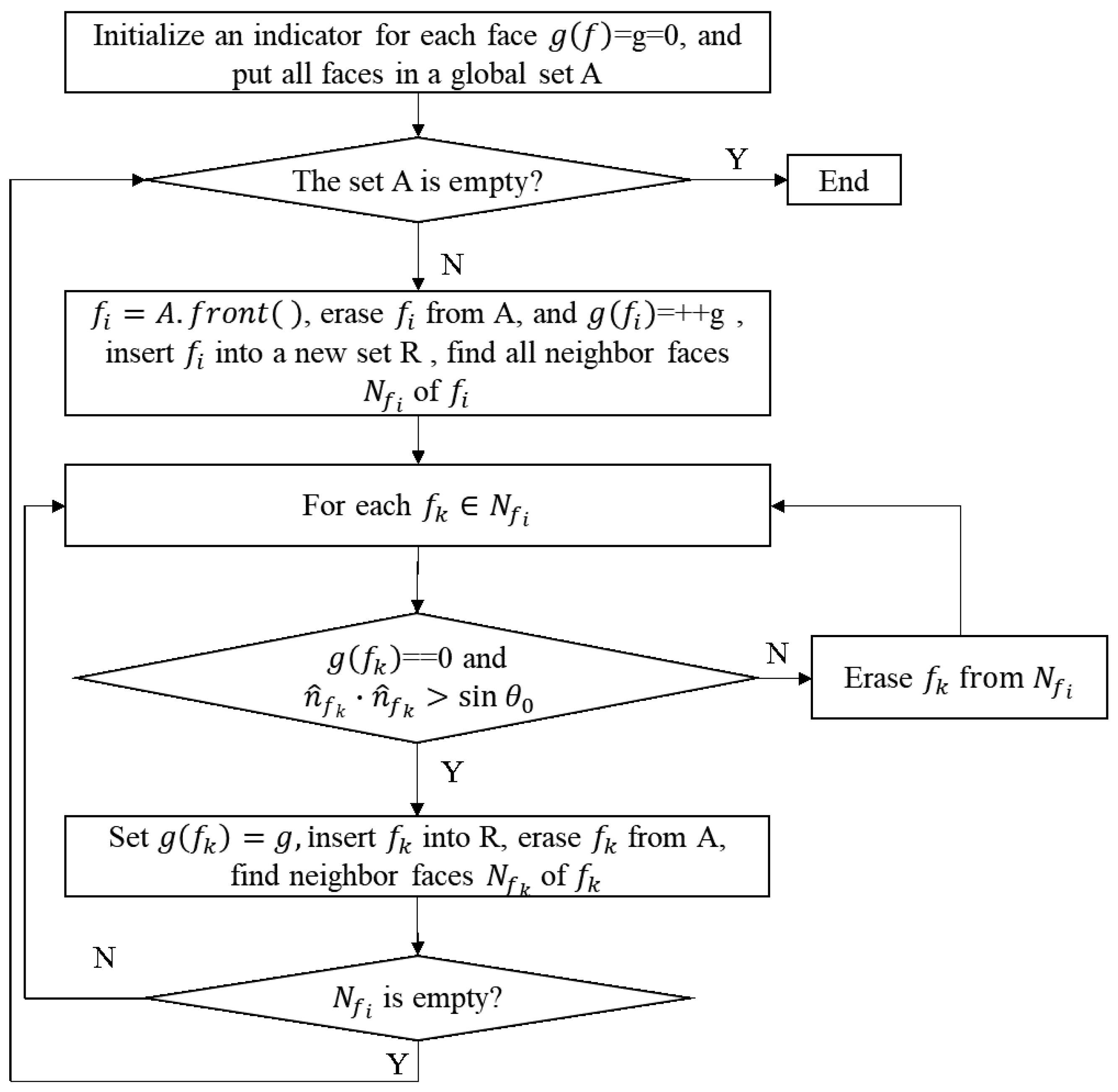
3.2.1. Region Growing
We obtain the plane detection results by using the region-growing algorithm. We select an ungrouped face and traverse neighboring faces to compare their normal orientations. If the orientations of two faces are similar, we merge them until there are no more faces with similar orientations. Finally, we get a set of coarse planar regions, and each face has been assigned to one of the regions [
37]. The detail of the region-growing algorithm is shown in
Figure 3.
3.2.2. Region Optimization
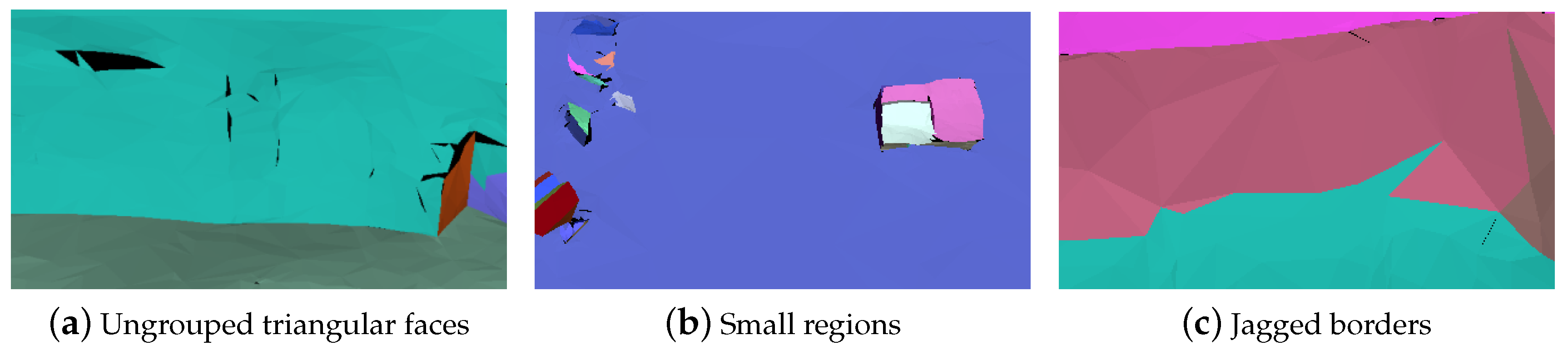
The region-growing algorithm generates a set of coarse planar regions. However, the shape detection results may be imperfect due to geometric noise and topological defects.
Figure 4 shows three common problems, and we summarize them as follows:
(1) Ungrouped triangular faces. The normal orientation of such a face differs from its neighboring faces, so it cannot be grouped into any regions.
(2) Small regions. The region-growing algorithm aims to detect the overall shapes of building models. Therefore, small regions should be grouped into the larger surrounding regions.
(3) Jagged borders. The boundaries of regions may appear jagged after growing, which further affects the subsequent simplification process.
Therefore, we perform region optimization to refine the shape detection results. For each problem mentioned above, specific approaches are designed. Ungrouped triangular faces are solved in the same way as small regions. We calculate the average normal orientations of their neighboring regions and group them into the region with the smallest angle. If the new region is still smaller than the threshold, each face in the region must be regrouped into one of its neighboring regions. We set a limitation that the minimum number of faces in a region should be no less than 10. For jagged borders, it is necessary to smooth such boundaries. We filter out boundary faces and then count the number of faces in the neighboring regions. Each boundary face is grouped into the region with more faces.
The optimized results of
Figure 4 are shown in
Figure 5.
Figure 6a,b display the full effect: (1) Rough planar regions are detected using the region-growing algorithm, but the shape detection results are imperfect due to noise. (2) Small regions have been grouped into neighboring regions according to our approaches.
3.3. Constraint Simplification
The basic principle of the edge-collapse algorithm is to merge the two vertices of an edge into one vertex and delete the edge and its two neighboring triangular faces. The algorithm decimates the input mesh according to a cost function until the desired simplification rate is reached. For the cost function, the QEM algorithm [
7] is a classic method for calculating the collapse cost, which uses the sum of the distance from a point to its neighboring faces as the error metric. The algorithm has been widely used because of its efficiency and quality of simplification. In the original QEM algorithm, each vertex is associated with a quadric matrix
. Given a face
, the squared distance from a vertex
to the face is:
Then, the sum of the squared distance from the vertex
v to all neighboring faces is:
For an edge
, the quadric matrix is computed by adding the quadrics of its two vertices, i.e.,
. Finally, we define the cost function of the edge
as:
where
is a new vertex.
The QEM algorithm can simplify general 3D models effectively. However, buildings have more planar regions with sharp features. If the original QEM algorithm is used for mesh simplification, these planar regions may get distorted, and the overall shapes may be destroyed by increasing the simplification rate. Therefore, we detect the typical shapes of buildings, perform simplification constrained by them, and preserve sharp features, such as edges and corners. It is worth noting that we need a balance between feature preservation and simplification efficiency.
We have predefined a set of planar regions in the previous step, and it is necessary to design the corresponding constraints on edges and corners. We classify vertices into three types and assign different weights according to the regions they belong to, as shown in
Figure 7 and
Figure 8. The faces, edges, and corners weights are set to 1, 10, and 100, respectively.
3.4. Texture Remapping
We adopt an automatic generation method for color models based on patch decomposition. This method simplifies a model without texture, divides the mesh into patches, remaps each patch with a lower resolution than the original model, and finally merges each patch’s texture to form a hierarchical simplified textured model. See patent [
38] for details.
4. Results and Discussions
4.1. Simplification Results
Figure 9 shows the results in the pipeline of the proposed method: mesh filtering, shape detection, and mesh simplification. Small regions are grouped into the larger surrounding regions for high-level simplification results. In total, the original model has 75,285 faces, while the simplified model remains 736 faces. The simplification ratio exceeds 99%, but the model still preserves the original appearance.
4.2. Qualitative and Quantitative Analysis
We compare the simplification results of a building model with a more complex structure. MeshLab is an open-source model processing software with many embedded simplification algorithms, and here we use the Quadric Edge Collapse function for comparison.
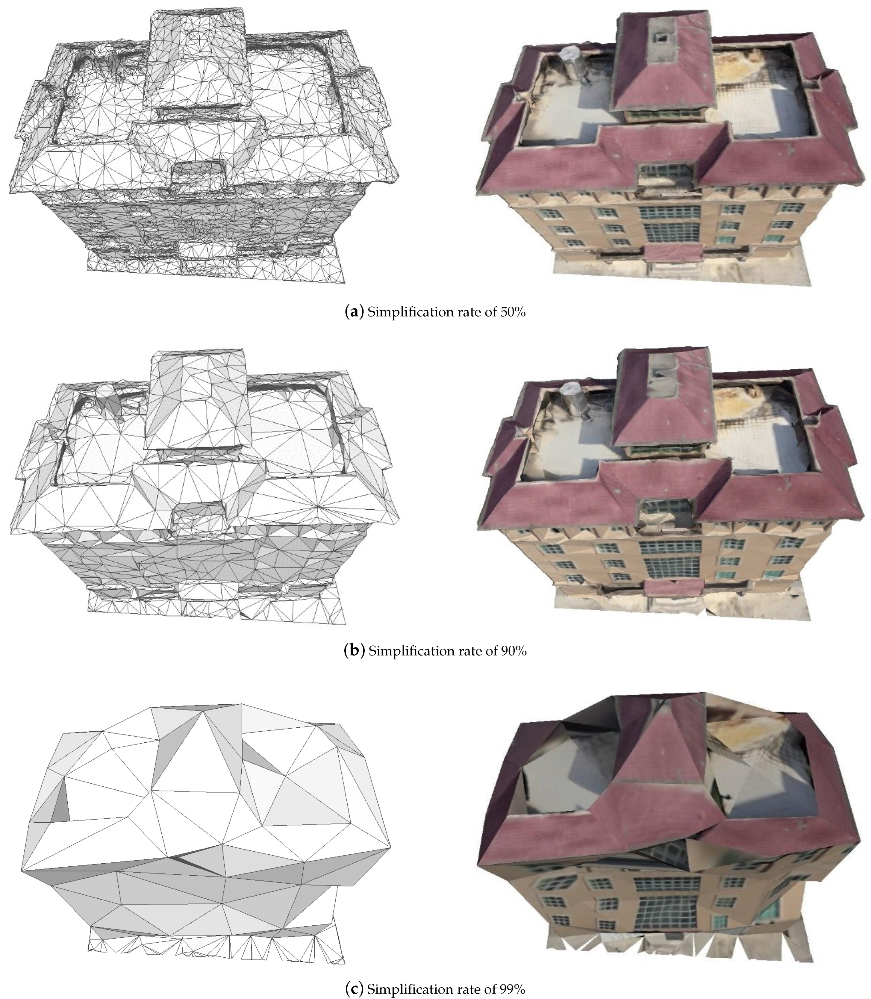
Figure 10 displays the original model, and
Figure 11 and
Figure 12 display the simplification results of the proposed method and the QEM algorithm when the simplification rates are 50%, 90%, and 99%, respectively. It can be seen from the results that the two methods can preserve the overall structure of the original model when the simplification rate is 50%. However, our method still preserves the appearance while the overall shape simplified by the QEM algorithm has been destroyed as the simplification rate increases, especially when it reaches 99%. Moreover, we remap the texture after the geometric simplification and compare it with the texture simplification method in MeshLab.
Except for the qualitative comparison, we also compare the results quantitatively. Here, we use the Hausdorff distance as the evaluation metric. It can be seen from
Table 1 that the simplification error of the QEM algorithm is a little lower than that of our method when the simplification rate is low. As the simplification ratio increases gradually, the advantage of our method is beginning to show. Especially when the simplification rate reaches 99%, the simplification error of our method is much lower than that of the QEM algorithm. We investigate the error curves and find out the cause of the difference. When the simplification rate is relatively low, the mesh retains plenty of triangular faces, so the simplification results of the two methods are not much different. However, we perform mesh filtering before simplification, slightly changing the original model’s appearance. Therefore, the simplification error of our method is a litter higher. With the simplification rate increasing, the structural features of the model will become less. The original QEM algorithm considers only local geometric features and decimates the mesh locally, leading to the distortion of the overall shape. Our method detects planar regions’ shapes, simplifies the mesh constrained by the detection results, and preserves sharp features, such as edges and corners. Because we assign higher weights to the non-planar regions, the planar regions are first simplified, which has little influence on the overall shape. Even with a much higher simplification rate, the edges and corners of the building are the last to be considered.
4.3. Comprehensive Analysis
We select an area of buildings for simplification comparison, as shown in
Figure 13. The original model has 1,841,516 faces, while the simplified model remains 4280 faces, where the simplification rate reaches 99.8%.
Figure 13b,c show the comparison between the simplified results of our method and the QEM algorithm. It can be seen from the figure that the result of the QEM algorithm has collapsed with broken and disordered triangular faces, and the corresponding texture is confused due to the geometric error. However, in the case of the same simplification rate, the overall shape distortion of the simplified model in this paper is within an acceptable range, and the texture remapping is also clearly discernible.
5. Conclusions
This paper proposes a simplified method that preserves the overall shapes of buildings in urban scenes. First, we preprocess mesh models by mesh filtering that refines the normal orientation of each triangular face and updates the corresponding vertex positions. The filtering process smooths planar regions while preserving sharp features, which further improves the performance of the subsequent simplification process. Then, we perform a region-growing algorithm on the models to detect the shapes of planar regions. After mesh filtering and shape detection, we develop the QEM algorithm for mesh simplification based on a hierarchical definition strategy of the error metric, which assigns different weights to the planar and non-planar regions. Finally, we adopt an automatic generation method for color models based on patch decomposition to obtain hierarchical simplified textured models. The experimental results show that compared to the original QEM algorithm, the proposed method can preserve the overall shapes of models, especially when the simplification rate is very high. However, the work of this paper has shortcomings. First, the ranges of regions and the weights of vertices are manually defined, which limits the method in this paper. Second, we do not fully utilize the semantic information of building models. How to carry out complete semantic modeling of buildings still requires investigation. In the future, the goal of simplification should be to associate the buildings at different levels according to geometry, topology, and semantics and to create a smoother transition in the visual sense between different levels.
Author Contributions
Conceptualization, Xianfeng Huang, Feng Lan and Fan Zhang; methodology, Hanyu Xiang, Feng Lan, Chong Yang, Yunlong Gao, Wenyu Wu and Fan Zhang; writing—original draft preparation, Hanyu Xiang and Feng Lan; writing—review and editing, Hanyu Xiang and Fan Zhang. All authors have read and agreed to the published version of the manuscript.
Funding
This research received no external funding.
Data Availability Statement
Not applicable.
Acknowledgments
This research is jointly supported by the National Key Research and Development Program of China (Grant No. 2020YFC1522703). The authors would like to thank the developers of CGAL and MeshLab.
Conflicts of Interest
The authors declare no conflict of interest.
References
- Li, M.; Nan, L. Feature-preserving 3D mesh simplification for urban buildings. ISPRS J. Photogramm. Remote Sens. 2021, 173, 135–150. [Google Scholar] [CrossRef]
- Biljecki, F.; Ledoux, H.; Stoter, J.; Zhao, J. Formalisation of the level of detail in 3D city modelling. Comput. Environ. Urban Syst. 2014, 48, 1–15. [Google Scholar] [CrossRef] [Green Version]
- Clark, J.H. Hierarchical geometric models for visible surface algorithms. Commun. ACM 1976, 19, 547–554. [Google Scholar] [CrossRef]
- Potamias, R.A.; Ploumpis, S.; Zafeiriou, S. Neural mesh simplification. In Proceedings of the IEEE/CVF Conference on Computer Vision and Pattern Recognition, Vancouver, BC, Canada, 18–24 June 2022; pp. 18583–18592. [Google Scholar]
- Salinas, D.; Lafarge, F.; Alliez, P. Structure-aware mesh decimation. Comput. Graph. Forum 2015, 34, 211–227. [Google Scholar] [CrossRef]
- Chang, R.; Butkiewicz, T.; Ziemkiewicz, C.; Wartell, Z.; Pollard, N.; Ribarsky, W. Legible simplification of textured urban models. IEEE Comput. Graph. Appl. 2008, 28, 27–36. [Google Scholar] [CrossRef] [Green Version]
- Garland, M.; Heckbert, P.S. Surface simplification using quadric error metrics. In Proceedings of the 24th Annual Conference on Computer Graphics and Interactive Techniques, Los Angeles, CA, USA, 3–8 August 1997; pp. 209–216. [Google Scholar]
- Garland, M.; Heckbert, P.S. Simplifying surfaces with color and texture using quadric error metrics. In Proceedings of the Visualization’98 (Cat. No.98CB36276), Research Triangle Park, NC, USA, 18–23 October 1998; pp. 263–269. [Google Scholar]
- Hoppe, H. New quadric metric for simplifying meshes with appearance attributes. In Proceedings of the Visualization’99 (Cat. No. 99CB37067), San Francisco, CA, USA, 24–29 October 1999; pp. 59–510. [Google Scholar]
- Liu, X.; Lin, L.; Wu, J.; Wang, W.; Yin, B.; Wang, C.C. Generating sparse self-supporting wireframe models for 3D printing using mesh simplification. Graph. Model. 2018, 98, 14–23. [Google Scholar] [CrossRef]
- Schroeder, W.J.; Zarge, J.A.; Lorensen, W.E. Decimation of triangle meshes. In Proceedings of the 19th Annual Conference on Computer Graphics and Interactive Techniques, Chicago, IL, USA, 26–31 July 1992; pp. 65–70. [Google Scholar]
- Renze, K.J.; Oliver, J.H. Generalized unstructured decimation. IEEE Comput. Graph. Appl. 1996, 16, 24–32. [Google Scholar] [CrossRef]
- Rossignac, J.; Borrel, P. Multi-resolution 3D approximations for rendering complex scenes. In Modeling in Computer Graphics; Springer: Berlin/Heidelberg, Germany, 1993; pp. 455–465. [Google Scholar]
- Low, K.L.; Tan, T.S. Model simplification using vertex-clustering. In Proceedings of the 1997 Symposium on Interactive 3D Graphics, Providence, RI, USA, 27–30 April 1997; pp. 75–81. [Google Scholar]
- Lounsbery, M.; DeRose, T.D.; Warren, J. Multiresolution analysis for surfaces of arbitrary topological type. ACM Trans. Graph. ToG 1997, 16, 34–73. [Google Scholar] [CrossRef]
- Guskov, I.; Vidimče, K.; Sweldens, W.; Schröder, P. Normal meshes. In Proceedings of the 27th Annual Conference on Computer Graphics and Interactive Techniques, New Orleans, LA, USA, 23–28 July 2000; pp. 95–102. [Google Scholar]
- Hoppe, H.; DeRose, T.; Duchamp, T.; McDonald, J.; Stuetzle, W. Mesh optimization. In Proceedings of the 20th Annual Conference on Computer Graphics and Interactive Techniques, Anaheim CA, USA, 2–6 August 1993; pp. 19–26. [Google Scholar]
- Hoppe, H.; DeRose, T.; Duchamp, T.; McDonald, J.; Stuetzle, W. Surface reconstruction from unorganized points. In Proceedings of the 19th Annual Conference on Computer Graphics and Interactive Techniques, Chicago, IL, USA, 26–31 July 1992; pp. 71–78. [Google Scholar]
- Kim, S.; Jeong, W.; Kim, C. LOD generation with discrete curvature error metric. In Proceedings of the Korea Israel Bi-National Conference, Seoul, Korea, 10–12 October 1999; pp. 97–104. [Google Scholar]
- Kim, S.J.; Kim, C.H.; Levin, D. Surface simplification using a discrete curvature norm. Comput. Graph. 2002, 26, 657–663. [Google Scholar] [CrossRef]
- Castelló, P.; Sbert, M.; Chover, M.; Feixas, M. Viewpoint-driven simplification using mutual information. Comput. Graph. 2008, 32, 451–463. [Google Scholar] [CrossRef]
- Lescoat, T.; Liu, H.T.D.; Thiery, J.M.; Jacobson, A.; Boubekeur, T.; Ovsjanikov, M. Spectral mesh simplification. Comput. Graph. Forum 2020, 39, 315–324. [Google Scholar] [CrossRef]
- Hoppe, H. Progressive meshes. In Proceedings of the 23rd Annual Conference on Computer Graphics and Interactive Techniques, New Orleans, LA, USA, 4–9 August 1996; pp. 99–108. [Google Scholar]
- Hoppe, H. View-dependent refinement of progressive meshes. In Proceedings of the 24th Annual Conference on Computer Graphics and Interactive Techniques, Los Angeles, CA, USA, 3–8 August 1997; pp. 189–198. [Google Scholar]
- Lindstrom, P.; Turk, G. Image-driven simplification. ACM Trans. Graph. (ToG) 2000, 19, 204–241. [Google Scholar] [CrossRef]
- Papageorgiou, A.; Platis, N. Triangular mesh simplification on the GPU. Vis. Comput. 2015, 31, 235–244. [Google Scholar] [CrossRef]
- Lee, H.; Kyung, M.H. Parallel mesh simplification using embedded tree collapsing. Vis. Comput. 2016, 32, 967–976. [Google Scholar] [CrossRef]
- Nan, L.; Wonka, P. Polyfit: Polygonal surface reconstruction from point clouds. In Proceedings of the IEEE International Conference on Computer Vision, Venice, Italy, 22–29 October 2017; pp. 2353–2361. [Google Scholar]
- She, J.; Gu, X.; Tan, J.; Tong, M.; Wang, C. An appearance-preserving simplification method for complex 3D building models. Trans. GIS 2019, 23, 275–293. [Google Scholar] [CrossRef]
- She, J.; Chen, B.; Tan, J.; Zhao, Q.; Ge, R. 3D building model simplification method considering both model mesh and building structure. Trans. GIS 2022, 26, 1182–1203. [Google Scholar] [CrossRef]
- Li, Q.; Sun, X.; Yang, B.; Jiang, S. Geometric structure simplification of 3D building models. ISPRS J. Photogramm. Remote Sens. 2013, 84, 100–113. [Google Scholar] [CrossRef]
- Wang, B.; Wu, G.; Zhao, Q.; Li, Y.; Gao, Y.; She, J. A Topology-Preserving Simplification Method for 3D Building Models. ISPRS Int. J. Geo-Inf. 2021, 10, 422. [Google Scholar] [CrossRef]
- Botsch, M.; Kobbelt, L.; Pauly, M.; Alliez, P.; Lévy, B. Polygon Mesh Processing; CRC Press: Boca Raton, FL, USA, 2010. [Google Scholar]
- Zheng, Y.; Fu, H.; Au, O.K.C.; Tai, C.L. Bilateral normal filtering for mesh denoising. IEEE Trans. Vis. Comput. Graph. 2010, 17, 1521–1530. [Google Scholar] [CrossRef]
- Taubin, G. Linear anisotropic mesh filtering. In IBM Research Report; IBM T.J. Watson Research Center: Yorktown Heights, NY, USA, 2001; Volume 1. [Google Scholar]
- Sun, X.; Rosin, P.L.; Martin, R.; Langbein, F. Fast and effective feature-preserving mesh denoising. IEEE Trans. Vis. Comput. Graph. 2007, 13, 925–938. [Google Scholar] [CrossRef]
- Lafarge, F.; Mallet, C. Creating large-scale city models from 3D-point clouds: A robust approach with hybrid representation. Int. J. Comput. Vis. 2012, 99, 69–85. [Google Scholar] [CrossRef] [Green Version]
- Huang, X.; Zhang, F.; Gao, Y. A Kind of Colored LOD Model Automatic Forming Method Decomposed Based on Block. China Patent CN109118588A, 25 September 2018. [Google Scholar]
Figure 1.
Pipeline of the proposed method.
Figure 1.
Pipeline of the proposed method.
Figure 2.
Comparison of the meshes before and after mesh filtering. (a) Original meshes. (b) Filtered meshes. (Left to Right) Partial models, face normals, and overall models.
Figure 2.
Comparison of the meshes before and after mesh filtering. (a) Original meshes. (b) Filtered meshes. (Left to Right) Partial models, face normals, and overall models.
Figure 3.
Pipeline of the region-growing algorithm.
Figure 3.
Pipeline of the region-growing algorithm.
Figure 4.
Examples of the common problems in the shape detection results. (a) Ungrouped triangular faces. (b) Small regions. (c) Jagged borders.
Figure 4.
Examples of the common problems in the shape detection results. (a) Ungrouped triangular faces. (b) Small regions. (c) Jagged borders.
Figure 5.
Optimized results of the examples in
Figure 4. (
a) Ungrouped triangular faces. (
b) Small regions. (
c) Jagged borders.
Figure 5.
Optimized results of the examples in
Figure 4. (
a) Ungrouped triangular faces. (
b) Small regions. (
c) Jagged borders.
Figure 6.
Comparison of the shape detection results before and after region optimization. (a) Coarse shape detection results. (b) Optimized shape detection results.
Figure 6.
Comparison of the shape detection results before and after region optimization. (a) Coarse shape detection results. (b) Optimized shape detection results.
Figure 7.
Types of vertices. (a) Vertices belong to one region. (b) Vertices belong to two regions. (c) Vertices belong to three regions.
Figure 7.
Types of vertices. (a) Vertices belong to one region. (b) Vertices belong to two regions. (c) Vertices belong to three regions.
Figure 8.
Types of edges. (a) Both vertices are of type V1. (b) One vertex is of type V1 and the other is of type V2. (c) Both vertices are of type V2.
Figure 8.
Types of edges. (a) Both vertices are of type V1. (b) One vertex is of type V1 and the other is of type V2. (c) Both vertices are of type V2.
Figure 9.
Examples of the results in the pipeline. (a) Original meshes (75,285 faces). (b) Filtered meshes. (c) Planar regions. (d) Simplified meshes (736 faces).
Figure 9.
Examples of the results in the pipeline. (a) Original meshes (75,285 faces). (b) Filtered meshes. (c) Planar regions. (d) Simplified meshes (736 faces).
Figure 10.
Original meshes (36,841 faces).
Figure 10.
Original meshes (36,841 faces).
Figure 11.
Simplified meshes in our method. (a) Simplification rate of 50% (36,841 faces). (b) Simplification rate of 90% (3682 faces). (c) Simplification rate of 99% (365 faces).
Figure 11.
Simplified meshes in our method. (a) Simplification rate of 50% (36,841 faces). (b) Simplification rate of 90% (3682 faces). (c) Simplification rate of 99% (365 faces).
Figure 12.
Simplified meshes in the QEM algorithm. (a) Simplification rate of 50% (36,841 faces). (b) Simplification rate of 90% (3682 faces). (c) Simplification rate of 99% (365 faces).
Figure 12.
Simplified meshes in the QEM algorithm. (a) Simplification rate of 50% (36,841 faces). (b) Simplification rate of 90% (3682 faces). (c) Simplification rate of 99% (365 faces).
Figure 13.
Comparison of the simplification results in our method and the QEM algorithm. (a) Original meshes (1,841,516 faces). (b) Simplified meshes in our method at the simplification rate of 99.8% (4280 faces). (c) Simplified meshes in the QEM algorithm at the simplification rate of 99.8% (4280 faces).
Table 1.
Quantitative comparison of our method and the QEM algorithm.
Table 1.
Quantitative comparison of our method and the QEM algorithm.
| Simplification Rates (%) | Our Method (cm) | QEM Algorithm (cm) |
|---|
| 10 | 0.0258 | 0.0262 |
| 20 | 0.0292 | 0.0281 |
| 30 | 0.0335 | 0.0363 |
| 40 | 0.0403 | 0.0459 |
| 50 | 0.0485 | 0.0451 |
| 60 | 0.0626 | 0.0620 |
| 70 | 0.0819 | 0.1131 |
| 80 | 0.1223 | 0.1754 |
| 90 | 0.2353 | 0.4287 |
| 95 | 0.4525 | 0.5731 |
| 99 | 2.2238 | 5.1416 |
| Publisher’s Note: MDPI stays neutral with regard to jurisdictional claims in published maps and institutional affiliations. |
© 2022 by the authors. Licensee MDPI, Basel, Switzerland. This article is an open access article distributed under the terms and conditions of the Creative Commons Attribution (CC BY) license (https://creativecommons.org/licenses/by/4.0/).


 ,
, 


