
DeepDBSCAN: Deep Density-Based Clustering for Geo-Tagged Photos
by
 , , ,
, , ,
Jang You Park
1,† ,
,
Dong June Ryu
2,†,
Kwang Woo Nam
2,*,†,
Insung Jang
3,
Minseok Jang
2 and
Yonsik Lee
2 1
Hanwha Systems Co., Ltd., Seoul 04541, Korea
2
Department of Computer and Information Engineering, Kunsan National University, Gunsan 54150, Korea
3
City & Geospatial ICT Research Section, Electronics and Telecommunications Research Institute (ETRI), Daejeon 34129, Korea
*
Author to whom correspondence should be addressed.
†
These authors contributed equally to this work.
ISPRS Int. J. Geo-Inf. 2021, 10(8), 548; https://doi.org/10.3390/ijgi10080548
Submission received: 21 May 2021
/
Revised: 4 August 2021
/
Accepted: 10 August 2021
/
Published: 14 August 2021
Abstract
:Density-based clustering algorithms have been the most commonly used algorithms for discovering regions and points of interest in cities using global positioning system (GPS) information in geo-tagged photos. However, users sometimes find more specific areas of interest using real objects captured in pictures. Recent advances in deep learning technology make it possible to recognize these objects in photos. However, since deep learning detection is a very time-consuming task, simply combining deep learning detection with density-based clustering is very costly. In this paper, we propose a novel algorithm supporting deep content and density-based clustering, called deep density-based spatial clustering of applications with noise (DeepDBSCAN). DeepDBSCAN incorporates object detection by deep learning into the density clustering algorithm using the nearest neighbor graph technique. Additionally, this supports a graph-based reduction algorithm that reduces the number of deep detections. We performed experiments with pictures shared by users on Flickr and compared the performance of multiple algorithms to demonstrate the excellence of the proposed algorithm.
1. Introduction
With recent advances in mobile devices, sharing geo-tagged photos has become popular on social network services such as Facebook, Twitter, and Instagram. Many researchers use geo-tagged photos to obtain interesting spatial and social knowledge. This knowledge is used in point-of-interest (POI) applications [1,2,3,4], trip recommendation services [5,6,7,8], social media management systems [9,10,11], etc. The most popular technique for such knowledge discovery is clustering by using the global positioning information (GPS) information in the photos. When researchers aim to discover clusters, many of them use density-based clustering algorithms such as density-based spatial clustering of applications with noise (DBSCAN) [12] and variants of this algorithm because they are very intuitive and support arbitrary shape clustering.
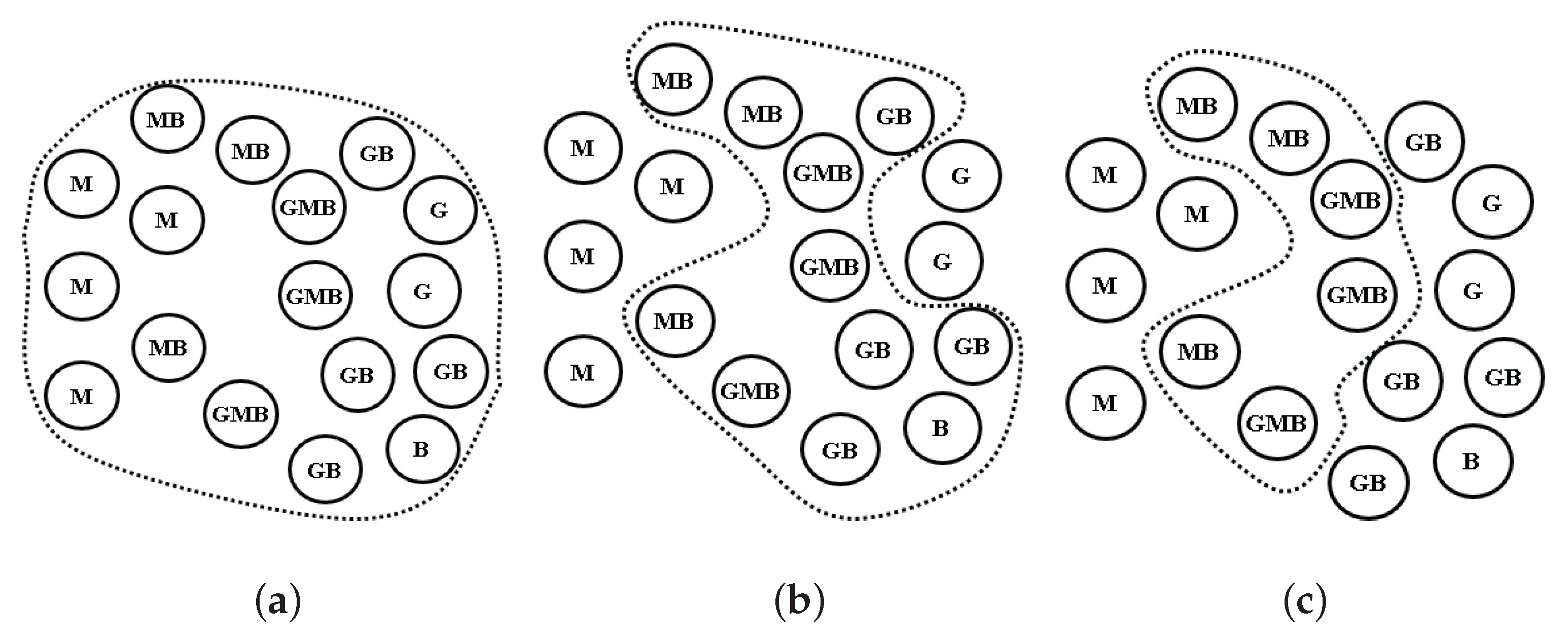
A geo-tagged photo contains the GPS information of the picture as well as in-depth content such as people, cars, trees, and animals. In obtaining knowledge, the objects that are in the photo are much more important than the location of the photo. Many applications, including POI recommendations, require in-depth clustering based on the content of the photo. However, most clustering algorithms have traditionally been used to construct clusters using only GPS information in geo-tagged photos, since recognizing objects in photographs and analyzing the relationships among them were very difficult problems before the recent progress in deep learning technology. Recently, researchers have been trying to discover POIs by applying these deep learning technologies [13,14]. Let us consider a case in which a researcher wants to find some POI clusters in social network photos taken around Yellowstone National Park. Figure 1 shows three examples of the results of density-based clustering with a spatial predicate without and with a deep content-based predicate. The traditional approach returns large clusters, as shown in Figure 1a because it is constructed from only the locations of the photos, irrespective of the contents of them. However, these queries are made very frequently in various application areas. Many systems already support aggregate functions. The following SQL code shows one of the most commonly used queries for density-based clustering of tour photos using a spatial predicate function ST_within(). This query selects only photos that were taken within Yellowstone National Park.
- SELECT id, DBSCAN(gps,eps:=50,mpts:=3) over() AS cid
- FROM tourPhotos
- WHERE ST_within(gps, $Yellowstone) AND IsDeepTrue(photo,‘Bear’,‘CNN_COCO’);
Furthermore, the above example contains a deep content-based predicate (deep predicate) function IsDeepTrue() that can select only photos containing specific animals through a given deep learning model. isDeepTrue (photo, ‘Bear’, ’CNN_COCO’) will select photos that contain bears using a convolutional neural network (CNN) model trained by the Microsoft COCO data set [15]. Integrating deep object detection with clustering queries could provide researchers with very powerful and convenient features in many applications. When they want to find only photos containing bears within a specific region, they can easily make this query by adding or changing the parameters in the deep and spatial predicate functions. Figure 1b,c show examples for the deep predicates ‘Bison’ and ’Bison AND Moose’, respectively. Despite the usefulness of these queries, studies so far have focused only on supporting the two functions. However, supporting these two functions together remains a performance-critical issue.
Deep content detection in photos is a very time-consuming task that takes a few seconds per photo, even on a modern computer system. Filtering spatial predicates and clustering the GPS locations of the photos are relatively fast tasks, and users often modify their parameters. Consequently, the traditional naive approach first performs deep content detection for all photos to construct a data set that has information about all objects detected in the photos in the batch preprocessing step. This data set can be inserted into a table in the database system or searched itself when the deep predicate is evaluated in the algorithm. This naive approach has many disadvantages. The most representative disadvantage is that deep detection is performed on all photos in advance. This is the least efficient method, considering that most photos do not meet the conditions of the density threshold or the spatial predicate. Since the deep detection task consumes a relatively large amount of computing time, we believe that minimizing the number of deep detections is the key to an efficient algorithm.
This paper proposes three novel algorithms to efficiently perform deep density-based clustering of geo-tagged photos.
- SpatialFirst DBSCAN: This algorithm performs spatialSelection first. We can reduce the number of deep detections by performing deep detection only on the spatially filtered results.
- ClusterFirst DBSCAN: Spatial selection and density-based clustering are performed in the first steps. Deep detection and selection are performed only on the photos in the clusters. However, we need to perform density-based clustering again only for photos that satisfy the deep predicate.
- DeepDBSCAN: Deep detection is performed by integrating it within the clustering algorithm. Deep detection is carefully performed on the nearest neighboring graph that satisfies the density threshold.
The rest of the paper is organized as follows: the related work is described in Section 2. In Section 3, we describe a naive algorithm for integrating deepSelection and density-based clustering as preliminaries. Section 4 presents the details of the three novel algorithms and examples. The experimental results using deep learning models are presented and discussed in Section 5. The conclusions and future work are described in Section 6.
2. Related Work
In this section, we review previous work including density-based clustering methods for discovering POIs and deep detection techniques.
2.1. Mining GPS and Trajectory Data
Recently, discovering user POIs has become very popular because POIs are the foundational data for location-based recommendations and advertisement services. Many studies have traditionally mined POIs from the GPS location and trajectory data of smart phones, vehicles, text, and photos. The earliest studies simply used location and time information to find a user’s favorite POIs [2]. The most common algorithms for POI discovery have been based on density-based clustering methods such as DBSCAN [12] and ST-DBSCAN [16]. Compared to the K-means algorithm, density-based clustering has been more widely used due to its advantages in discovering clusters with arbitrary shapes.
Another of these studies uses the GPS trajectories of objects to find their preferred routes [7] or groups [17] with similar patterns. However, GPS and trajectory data are very difficult to collect and analyze due to concerns such as privacy. In addition, this information does not provide rich information other than an object’s movement information. Therefore, research using geo-tagged photos has been conducted actively. In addition, various attempts are currently being made to improve the performance of density clustering algorithms. The most relevant of these studies is the G-DBSCAN [18] algorithm. They proposed a G-DBSCAN [18] which support GPU to solve computational and resource problems using graph algorithms such as depth-first and best-first traversal. We also propose a graph-based DBSCAN variant algorithm to increase performance by combining deep learning detection into DBSCAN algorithms. In this paper, we propose a branch pruning algorithm on the graph that can minimize the number of deep learning detection.
2.2. Mining Geo-Tagged Photos
With the development of mobile technology, users posting geo-tagged photos on social networks and sharing them has become a very generalized and natural social behavior. This has led researchers to a new opportunity. geo-tagged photos are provided voluntarily, with some even being publicly available for collection on social networks such as Flickr and Panoramio. Users can be identified by the ID provided with the photos, and a user’s travel path can be constructed from the ID. Furthermore, the photos show what the user is interested in specifically.
Early studies such as [8] focused on discovering tourist movement patterns in relation to regions of attraction (RoAs) and analyzing the topological characteristics of the travel routes of different tourists. Ref. [19] proposed a framework to automatically generate travel routes on Panoramio by crawling approximately 20 million geo-tagged photos and considering the time of the location information as well as the location information. In [20], an algorithm was presented to recommend tourist destination routes for specific regions in a Flickr photo data set. Refs. [21,22] went one step further and presented a fundamental method for finding the associated rules between POIs identified from geo-tagged photos. These studies commonly use density-based clustering as the underlying algorithm for discovering POIs. Photo DBSCAN (P-DBSCAN) [23] is the most commonly used technique for excluding photos frequently uploaded by the same user from social network photos. Recent studies have extended it to geo-tagged videos, such as [4,9,11].
Detecting the content of POIs was begun by analyzing the geo-tagged text of microblog data [24,25]. However, geo-tagged photos contain much more content than textual information. They even contain content that users did not intend, allowing the implicit meaning of POIs to be discovered. Recent advances in deep learning technology have made this possible. For example, object detection models such as You Only Look Once (YOLO) and RetinaNet can detect the location of an object with a bounding box [26,27]. Mask RCNN [28] supports pixel-level segmentation. These RCNN algorithms differ in their detection rates, and RCNN algorithms trained by Microsoft COCO data [15] can find and recognize 80 object categories in photos. Refs. [1,13] are good examples of studies that seek to apply deep learning technology to geo-tagged photos. In these studies, it is also essential to use density-based clustering to determine POIs. However, both papers use a naive algorithm that performs deep detection at the preprocessing stage.
3. Preliminaries
In this section, the naive method for content-based selection of geo-tagged photos is reviewed, and the limitations of this method are discussed. In general, the content-based selection of geo-tagged photos requires detection by a deep learning engine. Most systems utilize deep learning engines to detect images, which are configured separately from database queries and clustering algorithms. These systems perform image detection in batches using a deep learning engine for all stored geo-tagged photos, select photos that satisfy the image predicates, and then perform density-based clustering on these images. In other words, the naive approach is to perform image detection on the entire data set P and then to perform spatial filtering and clustering on the image data set that meets the image retrieval predicate (dp).
As shown in Algorithm 1, NaiveDBSCAN [12] requires an photo data set (P), a spatial predicate (sp) and deep content-based predicate (dp) as the input conditions and a radius () and minimum number of points (k), which are required to form a core in DBSCAN. The algorithm consists of four stages: deepSelection, spatialSelection, density-based nearest neighbor graph () construction, and cluster extension. The deepSelection function performs image detection and imagefiltering as the dp for the geo-tagged photo set P. It returns the photos that meet the dp criteria to . In the second step, the spatialSelection function performs spatial filtering, which satisfies the spatial condition sp for to extract the required data. In the third step, the constructNNGraph function is used to create an that has information about adjacent vertices that meet the density criteria () and the minimum number (k). The function constructNNGraph quickly uses spatial indexes to perform searches on adjacent vertices. Finally, expandCluster uses an to perform density-based clustering. The nearest neighbor graph () used in this algorithm can be defined as:
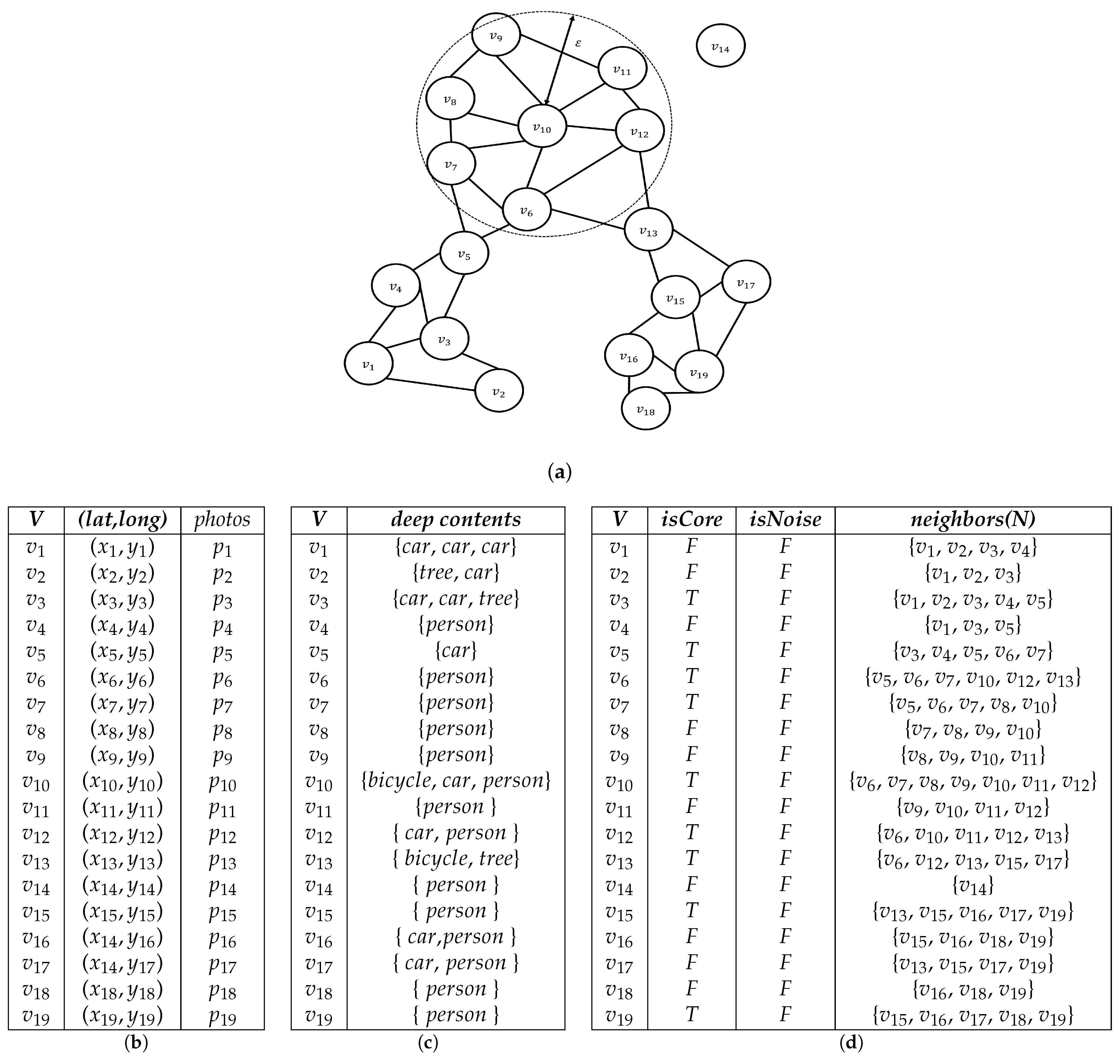
Given that V is a set of vertices v with coordinates x and y, where V = {, , …, }, and N is a set of subsets of V, is a set of pairs of a vertex in V and a set of neighboring vertices connected to that vertex. A connected neighbor vertex is a set of vertices that are within a radius of any vertex. NNG has auxiliary isCore and isNoise properties. Table 1 shows the symbols frequently used in this paper.
| Algorithm 1: NaiveDBSCAN. |
| Input: P, sc, dp, , k Output: 1 deepSelection(P, dp) 2 spatialSelection(, sc) 3 constructNNGraph(, , k) 4 expandCluster() 5return C |
Figure 2 shows an example of an . Set V contains all the vertices. Figure 2a plots the relationship between each vertex of V and the vertices within a certain radius of it. Figure 2c shows the contents of each vertex. For example, vertex has three cars. Vertices , , , and have both people and cars. Figure 2d is a table of vertices and their neighbors. Each of V’s vertices has a set of neighbors consisting of itself and its neighbors. If the number of neighbors at the vertex is greater than or equal to k, the vertex becomes the core vertex (T); otherwise, if it is less than k, it becomes boundary vertex (F). In other words, the vertex is the core vertex when . Figure 2d is an NNG graph table created when . Vertices , , , , , , , and have more than five neighbors. These vertices are the core vertices. If the clustering method’s minimum number of points is greater than five, core vertex and its neighbors become a cluster. Vertex does not form neighboring relationships with all vertices because no vertex is included within a certain radius. V’s vertices would comprise a cluster, as shown in Figure 1b, if dp were a person, considering content-based clustering.
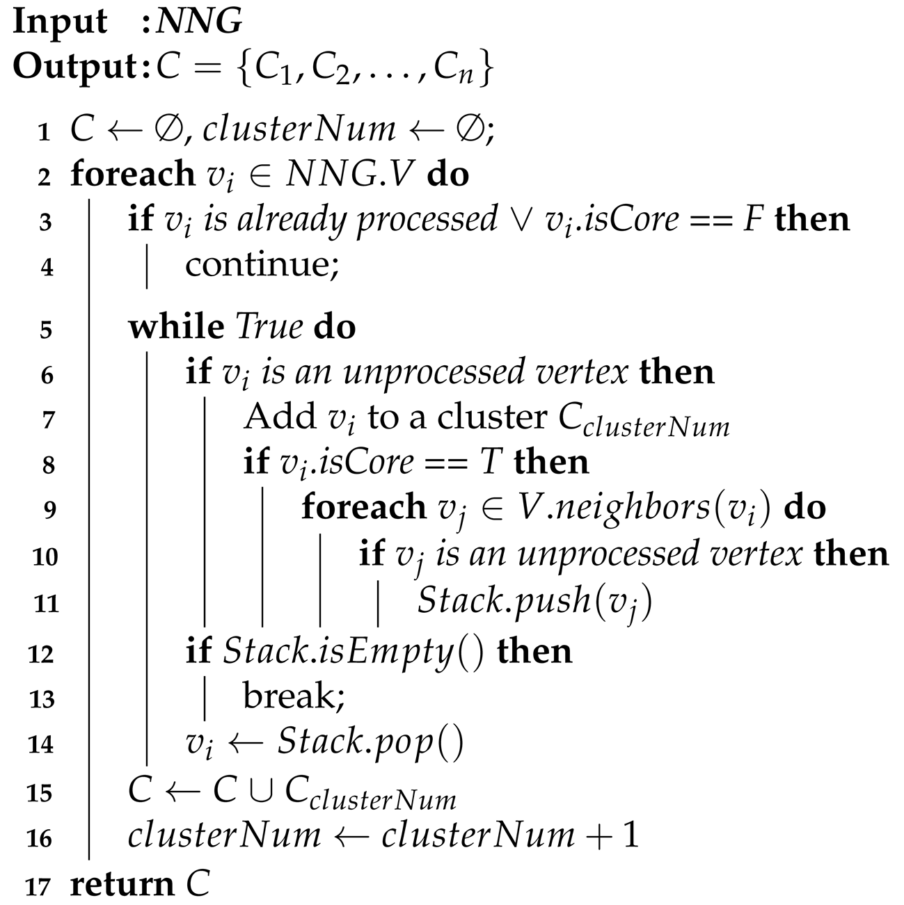
Algorithm 2 shows the expandCluster function as pseudocode. Algorithm 2 takes an as input and assigns cluster numbers to each vertex. That is, vertices are taken in order from the . The algorithm determines whether is a core vertex and assigns a cluster number to the core vertex and its neighbors. A core vertex is a vertex with more than k neighboring vertices within a radius of . Then, if the cluster contains other core vertices, it is recursively extended by assigning the same cluster number. This algorithm is identical to the existing DBSCAN algorithm except that it uses . All vertices in an are visited, and cluster numbers are assigned to core vertices that are not assigned cluster numbers or classified as noise. The same cluster number is assigned in recursively touring the neighboring vertices of the vertex that are core vertices and are assigned cluster numbers. This algorithm uses depth-first traversal algorithms using a stack for visits in the . If is a core vertex, V.neighbors() is used to select unprocessed vertices from the vertex’s neighbors, put them in a stack, and continue to extend them to neighboring vertices. When the visit to all the vertices in the stack is complete, the loop terminates. The cluster number is increased by 1 to build another cluster. The algorithm continues to visit the unvisited core vertices in the to expand the cluster. This task is performed repeatedly until all core vertices of the are visited. The total number of image detection by the naive method is equal to the number P, which sets all photos. The deepSelection function that recognizes images uses the most time, and an efficient way of dealing with this is required to reduce the cost.
| Algorithm 2: expandCluster. |
 |
4. Deep Content-Based Density Clustering
In this section, we propose a novel strategy to reduce the cost of image detection incurred by clustering techniques with deep learning models and DBSCAN.
4.1. Spatial-First Approach
The naive approach performs spatial filtering after image filtering. This is inefficient in terms of the time cost because performing image filtering takes more time than performing spatial filtering. Therefore, reducing the number of images used in performing image detection tasks has a significant impact on improving the time performance. Approaches that perform spatial filtering first import data from only a given spatial domain, so we can expect fewer image detection tasks than for naive approaches. Algorithm 3 is the pseudocode of a method that performs spatial filtering before image filtering.
| Algorithm 3: SpatialFirst DBSCAN. |
| Input: P, sp, dp, , k Output: 1 spatialSelection(P, sp) 2 deepSelection(, dp) 3 constructNNGraph(, , k) 4 expandCluster() 5return C |
The algorithm changes only the procedure of the functions deepSelection and spatialSelection in NaiveDBSCAN. The result of the two filters, , is the same. However, the number of images used in performing image filtering is the number of P in the naive method, whereas it is the number of in SpatialFirst DBSCAN.
Figure 3 shows the sequence of how SpatialFirst algorithms generate clusters. This figure shows the results of performing SpatialFirst algorithm based on data from Figure 2. Figure 3a shows queries for spatial predicates in a given initial state. After that, Figure 3b shows extract geo-tagged photos extracted from a given spatial area of the photo database. Figure 3c shows deepSelection results performed under the condition of the deep predicate ‘person’ for 19 extracted spatial pictures. At this point, four vertices , , , and that are dissatisfied with the given condition dp = ‘person’ are removed. Finally, Figure 3d shows the results of density-clustered based on k = 5. For vertices , , and , dp is satisfied but is removed when performing density clustering because it does not satisfy the number of neighbors k of each vertex. At this time, the number of image filtering for the algorithm is 19.
The time cost of the spatial-first algorithm can be expressed as follows:
where is a time cost of spatial selection, is a time cost of deepSelection, and is a time cost of density clustering including constructNNGGraph() and expandCluster() functions together.
This paper uses cost notation methods independent of implementation algorithms to simplify the cost comparison of the proposed algorithm. means a time cost that retrieves the photos satisfying given spatial predicate from a geo-tagged photo set P. When a spatial selection is implemented using spatial indexes, the cost will be . Sometimes, it is more efficient to implement it as a naive loop with than to use an spatial index under conditions with a large selectivity rate of . Regardless of how the spatial selection is implemented, the time cost is proportional to the size of the target data, as shown in the following equation:
where is a number of geo-tagged photos in P, and is a selectivity of a spatial predicate for P. When the selectivity for spatial predicate increases by 10 percent to 20 percent, the time costs will increase proportionately with or without the use of the index.
means a time cost to filter photos that satisfying the deep predicate from a data set by using a deep detection model. The time cost can be estimated approximately as the following equation:
where is a number of geo-tagged photos in , and is the average time taken to perform a deep detection on a single photo. In addition, can be represented by .
means a time cost to do density clustering for with the parameter and k. The density clustering can be implemented by various techniques with or as like grid-based or tree-based approaches. Therefore, we can represent the time cost as shown in the following equation:
where is a number of geo-tagged photos in . In addition, can be replaced by , where is a selectivity rate of .
4.2. Clustering-First Approach
The DBSCAN algorithm does not assign clusters to points that do not meet the conditions. Therefore, the points that are not allocated to a cluster are classified as noise. The clustering-first approach improves the algorithm’s performance by performing clustering before image filtering and not performing image filtering on the noise generated by clustering. Algorithm 4 is the pseudo code of the clustering-first approach.
The clustering-first approach consists of three steps. In the first step, we first select the photos that meet the spatial conditions and then perform spatialSelection and density clustering on these photos with only the GPS coordinates. In the second step, the clustering result C is converted into a data set, and image filtering is performed on only the images belonging to the cluster other than noise to generate . In the third step, the cluster is built by reclustering for only the set of images that meets the image detection criteria. The ClusterFirst algorithm performs less image detection than the SpatialFirst algorithm because it performs detection on images that have passed spatial density clustering except for the images classified as noise in the first step. This approach performs density clustering twice, which entails a greater clustering cost overhead. However, if the ratio of spatial density noise is high due to the low selectivity of the deep learning detection condition dp or if the distribution of the location of the photo data set is sparse, it will operate much more efficiently than the SpatialFirst algorithm.
| Algorithm 4: ClusterFirst DBSCAN. |
| Input: P, sp, dp, , k Output: 1 spatialSelection(P, sp) 2 constructNNGraph(, , k) 3 expandCluster() 4 deepSelection( flat(C), dp) 5 constructNNGraph(, ) 6 expandCluster() 7return |
Figure 4 shows the sequence of how ClusterFirst algorithms generate clusters based on Figure 2a. Figure 4a shows the results of generating an NNG graph under the condition of the minimum number of neighbors k within the vertex radius for geo-tagged photos satisfying a given spatial predicate (sp). At this point, the spatial predicate (sp) process for the specified data are skipped. Figure 4b shows the results of density-based clustering. For density-based clustering, outlier vertices are removed. Thus, we can see that has been removed. Figure 4c shows the result of deepSelection on the generated cluster. Figure 4c is the result of deleting geo-tagged photo that does not satisfy dp = ‘person’, such as (c) in Figure 3c. Figure 4d shows the result of density clustering. Vertices and do not become core vertexes due to dissatisfaction with the number of neighbors k, respectively. Therefore, it is removed at clustering time. In the case of ClusterFirst, image filtering is performed for all vertices in the nearest neighbor graph that satisfy the minimum number of neighbors k. However, when re-clustered, for an NNG graph with only vertices that meet dp, the vertices that do not satisfy the minimum number of neighbors k while vertices are removed.
The time cost of the clustering-first algorithm can be expressed as follows:
where is a time cost of spatial selection, is a time cost of first density clustering step for , is a time cost of deep selection for C, and is a time cost of the last density clustering step for .
The clustering-first algorithm performs pre-spatial density clustering step first to reduce the target data of time-dominant operation, and finally do a density clustering. For this reason, and are equivalent with Equations (2) and (4). First, means a time cost to do density clustering for with the parameter and k. Therefore, we can represent the time cost as shown in the following equation:
where is the number of geo-tagged photos in , and can be replaced by . In this equation, is equal with the number of target data in Equation (3). As a result, we can predict that will be equal to or less than that of (3) after .
means a time cost to filter photos that satisfying the deep predicate from a data set C by using a deep detection model. The time cost can be estimated approximately as the following equation:
where is a number of geo-tagged photos in C, is the average time taken to perform a deep detection on a single photo, and is a selectivity rate of Equation (6). Therefore, can be represented by .
In this equation, we can recognize that time cost is increased by processing , and decrease in proportion to . In another respect, if the is very large, the total time cost will be reduced in proportion to the amount of data reduced by even if the time cost is increased by processing . We will show that is very large enough to ignore the increase in in experiments using real data in Section 5.
4.3. DeepDBSCAN Approach
DeepDBSCAN is an approach that compensates for the shortcomings of the clustering-first approach by using the nearest neighbor graph technique. In the clustering-first approach described earlier, if the deep content-based predicate dp is not met, the vertex is a noise vertex, and the core vertex is sometimes dropped due to the failure to meet the minimum number of vertices used in the cluster creation condition k. In other words, dropped cores are vertices that do not meet k or dp. This dropped core can occur while traversing the NNG graph and affects neighborhood vertices when removed. When dropped cores affect core vertices that have not yet been visited, reducing the number of neighbors, and when the number of neighbors on those vertices is less than the minimum number of neighbors k, image filtering candidates can exclude neighbors from the vertex. Using this property, DeepDBSCAN first creates an NNG graph, then arranges the core vertex list in descending order by the vertices with the largest number of vertices, and performs image filtering on the vertices in the list and their neighbors. At this point, a core vertex that does not meet the dp condition may occur. If so, it removes groups that do not satisfy the minimum number of neighbors k, reflecting the relationship of the neighbor vertices being removed. It then traverses and performs image filtering until there are no unvisited core vertices.
Algorithm 5 shows pseudocode of DeepDBSCAN. Algorithm 5 has the same input parameters as Algorithm 4 described earlier and performs the same spatial filtering and generation. The NNG_DeepFiltering function removes noise from the that does not meet the dp while performing image detection on the vertices in the cluster. The noise is removed, resulting in a dropped core that does not satisfy the cluster conditions. Image filtering is not performed on the vertices in the dropped cores, improving the performance of the algorithm. This is described in detail in Algorithm 6. The that passes the filtering is clustered, and the results are returned.
| Algorithm 5: DeepDBSCAN. |
| Input: P, sp, dp, , k Output: 1 spatialSelection(P, sp) 2 constructNNGraph(, , k) 3 NNG_DeepFiltering(, dp, k) 4 expandCluster() 5return C |
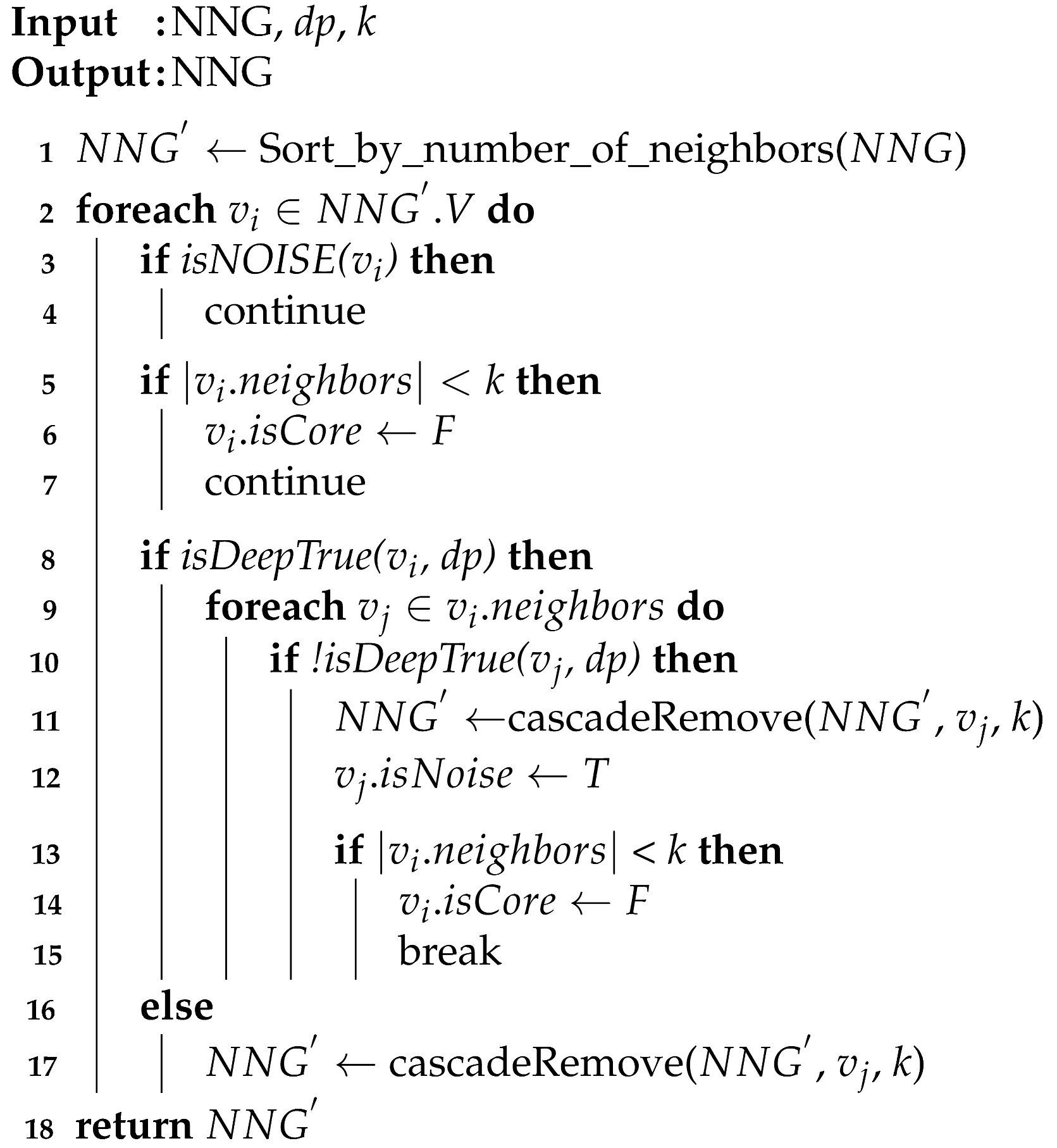
Algorithm 6 shows the pseudocode of the NNG_DeepFiltering function. The key goal of Algorithm 6 is to continue examining the cluster’s k condition while removing from the the noise vertices that do not satisfy the cluster’s deep content-based condition (). When a vertex does not satisfy the dp, it is considered “noise”.
Algorithm 6 first sorts the V in descending order based on the number of neighbors. The next step is to obtain the core vertices from and check the deep content-based predicate after the deep detection. The algorithm performs the algorithm on the next v vertex of the NNG graph without v being detected if the vertex v is a noise vertex, or if it has only v itself as a neighbor of v. Therefore, the function is defined:
Then, if the number of neighbors at the vertex is less than k, we switch the vertex to the boundary vertex and perform the algorithm on the next vertex. The DeepTrue function returns true when vertex satisfies the image predicate dp. If does not satisfy , it performs cascadeRemove function. The cascadeRemove function is described in Algorithm 7. If satisfies , the DeepTrue function is performed on the neighbor of . For vertices that do not satisfy dp for the neighboring vertex of , the cascadeRemove function is performed. Change ’s state to noise. If the number of neighbors in is less than k, is changed to not core. Finally, the graph is returned.
| Algorithm 6: NNG_DeepFiltering. |
 |
| Algorithm 7: cascadeRemove. |
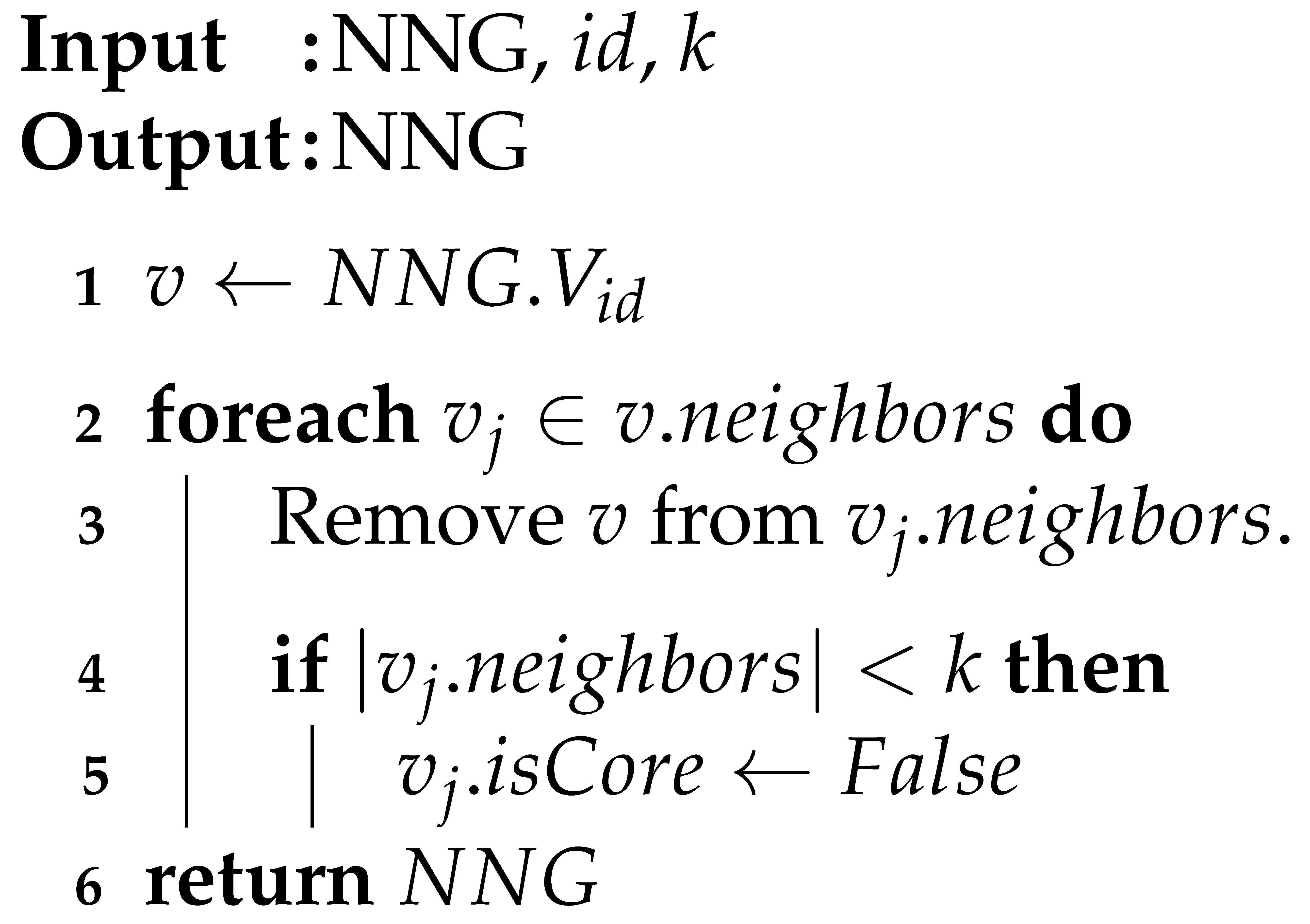 |
Algorithm 7 performs the removal of vertex v from v’s neighbors. The algorithm removes vertex v and uses vertex v as a neighbor to update the state of the number of neighbors on the other vertex to determine if it meets the minimum number of neighbors k and reflects that it is not a core vertex for a vertex . Finally, the NNG graph is returned.
The dropped cores occurred because there are fewer than five vertices that satisfy the ‘person’ condition. As such, if the core vertices fail to satisfy dp or if the core vertices satisfy dp but have noise vertices generated when passing through and detecting adjacent vertices one by one, we can improve the time-cost performance by switching to boundary vertices and excluding detections on these sub-graph. DeepDBSCAN, the cost reduction algorithm for content-based clustering proposed in this paper, improves the performance of the algorithm by excluding the vertices of the dropped core from image filtering.
As an example to help understand Algorithm 5, given NNG, as in Figure 2d, dp represents a ‘person’, and k is 5.
Table 2 is the result of sorting the V in the in Figure 2. The next step is to obtain the core vertices from and check the conditions for performing image filtering. The first core vertex is . The DeepTrue function returns a value of true when vertex satisfies the image predicate dp. The results of performing image filtering on images in satisfy dp = ‘person’. Then, all images are detected among ’s neighbors. All of ’s neighbors contain a ‘person’. next core vertex is . contains a person. Therefore, the DeepTrue function is performed on the neighbors of . The first neighbor of is , so is . There is no ‘person’ in the image of . Algorithm 7 is performed to remove from the NNG graph. In Algorithm 7, v is . From the neighbors of , is deleted and becomes a noise vertex.
Now, the information in is as follows:
| vertex | isCore | isNoise | neighbors |
| F | T | {, , , } |
Next, visit ’s neighbors and remove . Now, the information in , , , and is as follows:
| vertex | isCore | isNoise | neighbors |
| F | F | {, , , } | |
| F | F | {, , } | |
| T | F | {, , , , } | |
| F | F | {, , , } |
The next neighbor vertex of is . Image content of is unknown. Therefore, it performs object detection. There are no person in , so neighbor vertices of remove from the neighbors. At this point, has less than five neighbors, so it changes from core vertex to boundary vertex. After that, visit to perform image filtering and also perform image filtering for neighboring vertices to satisfy dp = ’person’ and terminate the algorithm.
Finally, Algorithm 6 is finished, is as shown in Table 3.
The vertices on which the algorithm performs image filtering are , , , , , , , , , , , , , and in order (14 total). Given the same condition k = 5 and dp = ‘person’, the ClusterFirst (CF) approach has 18 detections, but the DeepDBSCAN approach takes less time than the ClusterFirst approach because it has 14 detections.
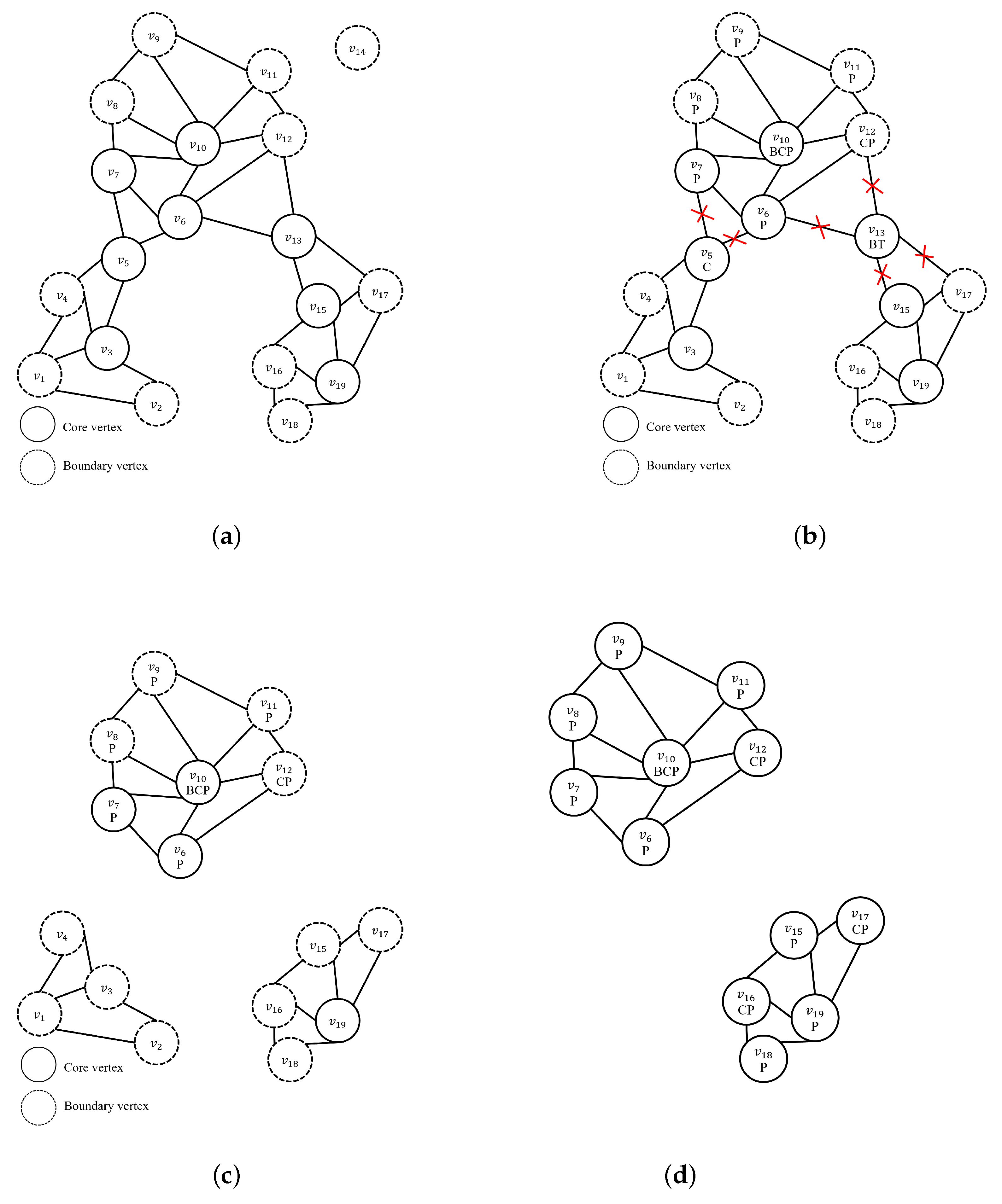
Figure 5 shows an example of DeepDBSCAN clustering when the minimum number of neighbor vertices is five (k = 5, dp = ‘person’). Figure 5a shows the results of the generated NNG graph based on k = 5. Vertices that satisfy number of neighbors k are marked core vertex, otherwise boundary vertex. In the table in Figure 2d, the vertices , , , , , , , and . have more than five (k = 5) neighbors, and they will be changed to core vertices and their neighbors changed to boundary vertices. The DeepDBSCAN approach visits the core vertices with the most neighborhood vertices in order to perform deep selection. Figure 5b shows the process of deep selection while traversing from the core vertex. At this time, when is performed on ’s neighbor vertices and , these vertices are dropped because they do not meet the dp condition.
Thus, the vertices dropped in Figure 5c show the effect on their neighbors. With removed, v4, v3 is the vertex at which the number of neighbors that have not been visited is adjusted. is also removed and affects the number of neighbors in and . We can see that is not satisfied with the number of k neighbors by removing . DeepDBSCAN does not perform deep selection on a sub-graph that does not have core vertices. Therefore, , , , and are excluded from the image filtering candidates. The next core vertex is . satisfies dp, and it performs image detection for neighborhood vertices of . Figure 5d shows the results after density clustering. The results are the same as those of the SpatialFirst and ClusterFirst algorithms shown earlier but show that the number of image detection is less. Consequently, the vertices that can construct clusters in the table in Figure 2d are , , , , , , , , and . Of these vertices, , , , , , , and do not include ‘person’ between neighbors. Thus, , , , , , , and are removed from the core vertex, resulting in a sub-graph that does not satisfy the number of neighbors K. Our algorithm improves performance by excluding these sub-graphs from the deep selection candidates.
The time cost of the DeepDBSCAN algorithm can be expressed as follows:
where is a time cost of spatialSelection, is a time cost of the constructNNGraph() function for , is a time cost of deepSelection and filtering it on the given graph , and is a time cost of the expandCluster() function for .
The DeepDBSCAN algorithm has two major differences in view of time cost. First, we divide into and since the in Equation (6) is total cost of constructNNGraph() and expandCluster() functions. Second, while in Equation (3) is a naive loop implementation, is performed under the conditions of minimum k on the given graph . We expect that the complexity will be improved to for the time cost for deepSelection step.
Using new representation and , the time cost of the clustering-first algorithm can be expressed as follows:
When Equation (8) is compared with Equation (9), we can find that , , and are the same as those of Equation (9). Since the NNG_DeepFiltering() algorithm is implemented by integrating and , it is clear that the time cost of is equal to or less than the sum of and . For this reason, it is clear that the following equation is true:
5. Experiments and Evaluation
In this section, we evaluate the performance of the proposed DeepDBSCAN algorithm. Three algorithms, SpatialFirst ClusterFirst and DeepDBSCAN, are compared. Each algorithm is also tested to determine the settings of and k that affect the DBSCAN results.
5.1. Experimental Setup
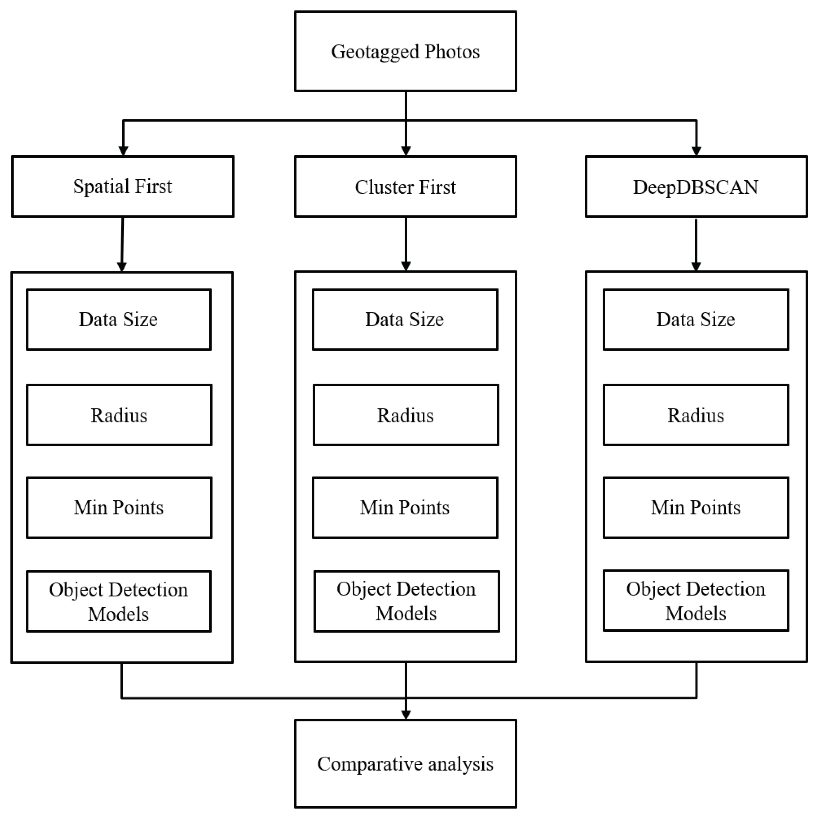
We collected photos containing geographical information from Flickr.com to use actual geographical data. Approximately 180,000 photos were collected around the densely populated city of New York. We prepared a data set of 10,000 photos in increments of 10,000 to 50,000 close to the central coordinates.The central coordinates (latitude: 40.783294, longitude: −73.96453) were set near Times Square for experiments. The algorithm used in the experiment was implemented in Python on Windows 10. All experiments were performed on an Intel i7-4770 3.40 GHz 4-core CPU with 16 GB RAM and RTX 2080ti. Figure 6 shows our experimental setup. we chose three different evaluation aspects in the comparative analysis with three different algorithms (SpatialFirst, ClusterFirst, DeepDBSCAN). We experimented with (1) the effect of the data size on performance, (2) the effect of the radius on performance, and (3) the effect of a minimum number of points on performance and evaluated these configurations. We measured the execution speed of the algorithm to evaluate the performance of the algorithm. For comparison, we used several object detection models. We adopted Yolo [26], Mask RCNN [28], and RetinaNet [27] for object detection models trained with the Microsoft COCO data set [15].
5.2. Effect of the Data Size
The first experiment evaluated the effect of the data size on the performance of the algorithms. The performance measurement was the computational cost of the algorithms. We experimented by fixing the radius at 100 m, varying the minpts among 9, 15, and 21 and varying the data size from 10,000 to 50,000. Figure 7a–c show the count of image filtering by SpatialFirst (SF), ClusterFirst (CF), and DeepDBSCAN as the data size changes. Figure 7d–f show the times spent for each detection model to perform image filtering. At this time, SF was excluded from the comparison due to the large number of images to filter. The table below the figure shows the time spent for each algorithm, depending on the variation in data size. This is based on the Mask RCNN, which spent the most time filtering images. The runtime of all algorithms increases as the data size increases. The number of image detection is in the order of SpatialFirstClusterFirst and DeepDBSCAN. The SpatialFirst performs image detection on all data, and ClusterFirst performs image detection less than SpatialFirst because noise data were deleted during creation and clustering. DeepDBSCAN seems to have a similar number of image detections to ClusterFirst, but, as the data size increases, we can see that it performs an amount of image detection about 3% less as more vertices are excluded. Although ClusterFirst and DeepDBSCAN have shorter running times compared to SpatialFirst and DeepDBSCAN and ClusterFirst have similar running times, we can see that DeepDBSCAN is better.
5.3. Effect of the Radius
The second experiment evaluated the effect of the radius on the performance of the algorithms. The performance measurement is the computational cost of the algorithms. We experimented by fixing the data size at 10,000 and varying minpts among 9, 15, and 21 and the radius from 100 m to 500 m. Figure 8a–c show how the algorithms’ performance times change as the radius of the cluster changes. Figure 8d–f depict the times spent for each detection model to perform image filtering. The SpatialFirst algorithm was excluded for the same reason. The table below the figure presents the time spent for each algorithm, depending on the variation in radius. It is written based on Mask RCNN, as shown in the table in Figure 7. The SpatialFirst algorithm always has consistent run times, while the ClusterFirst and DeepDBSCAN run times increase as the radius grows. This is because the larger the radius of a cluster is, the more photos it contains and the more candidates it needs in order to filter images. On the other hand, as the minimum number of vertices forming a cluster increases, fewer candidates are required to form fewer clusters and perform image filtering. We can see that DeepDBSCAN outperforms ClusterFirst and SpatialFirst.
5.4. Effect of the Minimum Number of Points
The third experiment evaluated the effect of the minimum number of points on the performance of the algorithms. The performance measurement is the computational cost of the algorithms. We experimented by fixing the data size at 10,000 and varying minpts from 9 to 21. The radii varied from 100 m to 500 m. Figure 9a–c depict how the performance time changes as the minimum number of points in the cluster changes. Figure 9d–f show the times spent for each detection model to perform image filtering. The SpatialFirst algorithm was excluded for the same reason. The table below the figure presents the time spent for each algorithm, depending on the variation in radius. It is written based on Mask RCNN, as shown in the table in Figure 7.
As the minimum number of points forming the cluster increases, fewer candidates are required to form clusters and perform image detection. The number of photos needed in filtering the image candidates decreases as minpts increases. The SpatialFirst algorithm always has the same run time, while ClusterFirst and DeepDBSCAN show decreased run times as minpts increases. Additionally, in Figure 9, the DeepDBSCAN algorithm shows the best performance. We compared the impact of data size, cluster radius, and minimum points on the DBSCAN clustering algorithm based on the running time of each algorithm. We compared the running time required to perform image filtering using RCNN models for the vertices of the cluster that Rare formed. The proposed DeepDBSCAN algorithm performed well in all comparison groups. Additionally, if we add conditions for the number of people in the image, we can reduce image detection and show better performance.
6. Case Study
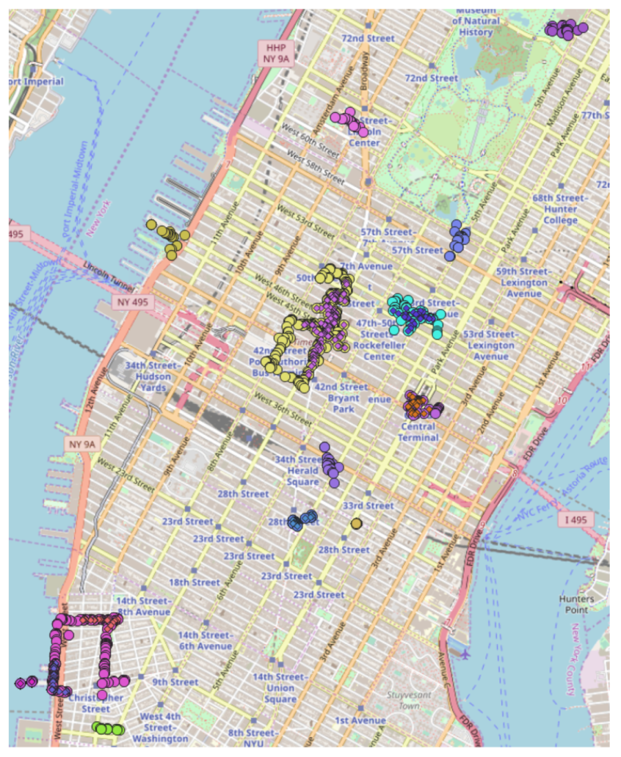
Figure 10 shows example of experimental data and the difference between traditional DBSCAN and image content-based DBSCAN. The image filtering condition was selected as a photograph of a person in order to find out whether it is possible to cluster a region with a lot of human traffic from a marketing point of view. The data used geo-tagged photos of the space near Times Square. The circle points are clusters, and different colors separate each cluster. The circle points and the diamonds in the circle points show the results of normal DBSCAN and DBSCAN based on the image contents. If we add the number of people in the image as a condition, we can exclude more sub-graphs. It can also reduce the number of core vertices compared to before. As the number of core vertices decreases, so does the number of image detection candidates decreases. This reduces computing costs and resources used and more accurately identifies areas of high person density in key regions. It can be seen that image content-based clusters can be useful in areas such as marketing by clustering places with high traffic.
7. Conclusions
We present deep content and density-based clustering techniques for geo-tagged photos. Content-based clustering of geo-tagged photos enables the discovery of POIs based on the locations of the geo-tagged images and enables searching of specific classes by leveraging deep learning models. This is used to detect hotspots and to search for specific classes in a particular region. In that sense, since spatial image data sets are stored in large quantities in systems such as databases, the time taken to discover a particular class of regions of interest is added to the existing DBSCAN techniques, as is the time spent on image detection tasks. The detection of images is highly time consuming. In this paper, we introduce three approaches to image content and clustering analysis techniques. In the case of the SpatialFirst algorithm, image detection is performed for all photo data in the region. To improve this, we introduce a ClusterFirst algorithm that eliminates outliers and performs object detection in the process of generating clusters based on geo-tagged photos in the spatial domain. Nevertheless, there are cases where object detection needs to be performed on the image even though there is no image containing dp(deep predicate). To solve this problem, we propose a deep density-based clustering (DeepDBSCAN) algorithm to reduce geo-tagged photo using nearest neighbor graph techniques. The key idea of DeepDBSCAN is to reduce the amount of image data used for image filtering by filtering clusters that do not satisfy certain conditions by considering space-based clustering and image detection predicates. Comparative experiments with several RCNN models, proposed algorithms, and previous algorithms show that it is important to reduce the number of image data when evaluating the time performance of image filtering. Our proposed DeepDBSCAN performs image detection approximately 5% less time on average than traditional methods. Therefore, it shows better performance in terms of time cost. As a result, our algorithm can find regions that satisfy image content and spatial conditions faster than traditional methods.
Author Contributions
Conceptualization, Insung Jang; methodology, Minseok Jang; software, Jang You Park and Dong June Ryu; validation, Minseok Jang; formal analysis, Kwang Woo Nam; investigation, Yonsik Lee; resources, Minseok Jang; data curation, Insung Jang; writing—original draft preparation, Jang You Park; writing—review and editing, Dong June Ryu and Kwang Woo Nam; project administration, Kwang Woo Nam; funding acquisition, Kwang Woo Nam, Insung Jang and Yonsik Lee. All authors have read and agreed to the published version of the manuscript.
Funding
This work was supported by an Electronics and Telecommunications Research Institute (ETRI) grant funded by the Korean government (21ZR1200, DNA-based national intelligence core technology development), and by the National Research Foundation of Korea (NRF) grant funded by the Korea government (MSIT) (No. 2018R1A2B6007982, No. 2021R1F1A1047768, and No. 2020R1F1A1048432).
Institutional Review Board Statement
Not applicable.
Informed Consent Statement
Not applicable.
Conflicts of Interest
The authors declare no conflict of interest.
References
- Kim, D.; Kang, Y.; Park, Y.; Kim, N.; Lee, J. Understanding tourists’ urban images with geotagged photos using convolutional neural networks. Spat. Inf. Res. 2020, 28, 241–255. [Google Scholar] [CrossRef] [Green Version]
- Kisilevich, S.; Keim, D.; Andrienko, N.; Andrienko, G. Towards acquisition of semantics of places and events by multi-perspective analysis of geotagged photo collections. In Geospatial Visualisation; Springer: Berlin/Heidelberg, Germany, 2013; pp. 211–233. [Google Scholar]
- Tian, J.; Ding, W.; Wu, C.; Nam, K.W. A Generalized Approach for Anomaly Detection From the Internet of Moving Things. IEEE Access 2019, 7, 144972–144982. [Google Scholar] [CrossRef]
- Ding, W.; Yang, K.; Nam, K.W. Measuring similarity between geo-tagged videos using largest common view. Electron. Lett. 2019, 55, 450–452. [Google Scholar] [CrossRef] [Green Version]
- Zeng, Z.; Zhang, R.; Liu, X.; Guo, X.; Sun, H. Generating tourism path from trajectories and geo-photos. In Proceedings of the International Conference on Web Information Systems Engineering, Doha, Qatar, 13–15 November 2012; Springer: Berlin/Heidelberg, Germany, 2012; pp. 199–212. [Google Scholar]
- Kurashima, T.; Iwata, T.; Irie, G.; Fujimura, K. Travel route recommendation using geotags in photo sharing sites. In Proceedings of the 19th ACM International Conference on Information and Knowledge Management, Toronto, ON, Canada, 26–30 October 2010; pp. 579–588. [Google Scholar]
- Chen, Y.Y.; Cheng, A.J.; Hsu, W.H. Travel recommendation by mining people attributes and travel group types from community-contributed photos. IEEE Trans. Multimed. 2013, 15, 1283–1295. [Google Scholar] [CrossRef]
- Zheng, Y.T.; Zha, Z.J.; Chua, T.S. Mining travel patterns from geotagged photos. ACM Trans. Intell. Syst. Technol. (TIST) 2012, 3, 1–18. [Google Scholar] [CrossRef]
- Kim, Y.; Kim, J.; Yu, H. Geotree: Using spatial information for georeferenced video search. Knowl.-Based Syst. 2014, 61, 1–12. [Google Scholar] [CrossRef]
- Kim, S.H.; Lu, Y.; Constantinou, G.; Shahabi, C.; Wang, G.; Zimmermann, R. Mediaq: Mobile multimedia management system. In Proceedings of the 5th ACM Multimedia Systems Conference, Singapore, 19–21 March 2014; pp. 224–235. [Google Scholar]
- Lu, Y.; To, H.; Alfarrarjeh, A.; Kim, S.H.; Yin, Y.; Zimmermann, R.; Shahabi, C. GeoUGV: User-generated mobile video dataset with fine granularity spatial metadata. In Proceedings of the 7th International Conference on Multimedia Systems, Klagenfurt, Austria, 10–13 May 2016; pp. 1–6. [Google Scholar]
- Ester, M.; Kriegel, H.P.; Sander, J.; Xu, X. A density-Based Algorithm for Discovering Clusters in Large Spatial Databases with Noise; KDD: Washington, DC, USA, 1996; Volume 96, pp. 226–231. [Google Scholar]
- Chang, B.; Park, Y.; Kim, S.; Kang, J. DeepPIM: A deep neural point-of-interest imputation model. Inf. Sci. 2018, 465, 61–71. [Google Scholar] [CrossRef]
- Zhang, S.; Yao, L.; Sun, A.; Tay, Y. Deep learning based recommender system: A survey and new perspectives. ACM Comput. Surv. (CSUR) 2019, 52, 1–38. [Google Scholar] [CrossRef] [Green Version]
- Lin, T.Y.; Maire, M.; Belongie, S.; Hays, J.; Perona, P.; Ramanan, D.; Dollár, P.; Zitnick, C.L. Microsoft coco: Common objects in context. In Proceedings of the European Conference on Computer Vision, Zurich, Switzerland, 6–12 September 2014; Springer: Berlin/Heidelberg, Germany, 2014; pp. 740–755. [Google Scholar]
- Birant, D.; Kut, A. ST-DBSCAN: An algorithm for clustering spatial–temporal data. Data Knowl. Eng. 2007, 60, 208–221. [Google Scholar] [CrossRef]
- Li, Z.; Han, J.; Ji, M.; Tang, L.A.; Yu, Y.; Ding, B.; Lee, J.G.; Kays, R. Fast mining of spatial frequent wordset from social database. ACM Trans. Intell. Syst. Technol. 2011, 2, 1–32. [Google Scholar]
- Andrade, G.; Ramos, G.; Madeira, D.; Sachetto, R.; Ferreira, R.; Rocha, L. G-dbscan: A gpu accelerated algorithm for density-based clustering. Procedia Comput. Sci. 2013, 18, 369–378. [Google Scholar] [CrossRef] [Green Version]
- Yin, H.; Wang, C.; Yu, N.; Zhang, L. Trip mining and recommendation from geo-tagged photos. In Proceedings of the 2012 IEEE International Conference on Multimedia and Expo Workshops, Melbourne, VIC, Australia, 9–13 July 2012; pp. 540–545. [Google Scholar]
- Spyrou, E.; Sofianos, I.; Mylonas, P. Mining tourist routes from Flickr photos. In Proceedings of the 2015 10th International Workshop on Semantic and Social Media Adaptation and Personalization (SMAP), Trento, Italy, 5–6 November 2015; pp. 1–5. [Google Scholar]
- Lee, I.; Cai, G.; Lee, K. Mining points-of-interest association rules from geo-tagged photos. In Proceedings of the 2013 46th Hawaii International Conference on System Sciences, Wailea, HI, USA, 7–10 January 2013; pp. 1580–1588. [Google Scholar]
- Zou, Z.; He, X.; Xie, X.; Huang, Q. Enhancing the Impression on Cities: Mining Relations of Attractions with Geo-Tagged Photos. In Proceedings of the 2018 IEEE SmartWorld, Ubiquitous Intelligence & Computing, Advanced & Trusted Computing, Scalable Computing & Communications, Cloud & Big Data Computing, Internet of People and Smart City Innovation, Guangzhou, China, 8–12 October 2018; pp. 1718–1724. [Google Scholar]
- Kisilevich, S.; Mansmann, F.; Keim, D. P-DBSCAN: A density based clustering algorithm for exploration and analysis of attractive areas using collections of geo-tagged photos. In Proceedings of the 1st International Conference and Exhibition on Computing for Geospatial Research & Application, Washington, DC, USA, 21–23 June 2010; pp. 1–4. [Google Scholar]
- Weng, J.; Lee, B.S. Event detection in twitter. In Proceedings of the International AAAI Conference on Web and Social Media, Barcelona, Spain, 17–21 July 2011; Volume 5. [Google Scholar]
- Lee, Y.; Nam, K.W.; Ryu, K.H. Fast mining of spatial frequent wordset from social database. Spat. Inf. Res. 2017, 25, 271–280. [Google Scholar] [CrossRef] [Green Version]
- Redmon, J.; Farhadi, A. Yolov3: An incremental improvement. arXiv 2018, arXiv:1804.02767. [Google Scholar]
- Lin, T.Y.; Goyal, P.; Girshick, R.; He, K.; Dollár, P. Focal loss for dense object detection. In Proceedings of the IEEE International Conference on Computer Vision, Venice, Italy, 22–29 October 2017; pp. 2980–2988. [Google Scholar]
- He, K.; Gkioxari, G.; Dollár, P.; Girshick, R. Mask r-cnn. In Proceedings of the IEEE International Conference on Computer Vision, Venice, Italy, 22–29 October 2017; pp. 2961–2969. [Google Scholar]
Figure 1.
Examples of traditional and deep density-based clustering of the geo-tagged photos (M = Moose, B = Bison, and G = Grizzly Bear in Yellowstone National Park). (a) only spatial predicate; (b) a spatial predicate and a deep predicate ‘Bison’; (c) a spatial predicate and a deep predicate ‘Bison AND Moose’.

Figure 2.
Example of a nearest neighbor graph. (a) -nearest neighbors graph; (b) geo-tagged photos table, P; (c) real deep contents table; (d) initial nearest neighbor graph, NNG.
Figure 2.
Example of a nearest neighbor graph. (a) -nearest neighbors graph; (b) geo-tagged photos table, P; (c) real deep contents table; (d) initial nearest neighbor graph, NNG.

Figure 3.
An example of SpatialFirst DBSCAN. (a) initial state and spatial predicate; (b) after spatialSelection; (c) after deepSelection (dp = ‘person’); (d) after constructNNGGraph (k = 5). and density clustering.
Figure 3.
An example of SpatialFirst DBSCAN. (a) initial state and spatial predicate; (b) after spatialSelection; (c) after deepSelection (dp = ‘person’); (d) after constructNNGGraph (k = 5). and density clustering.
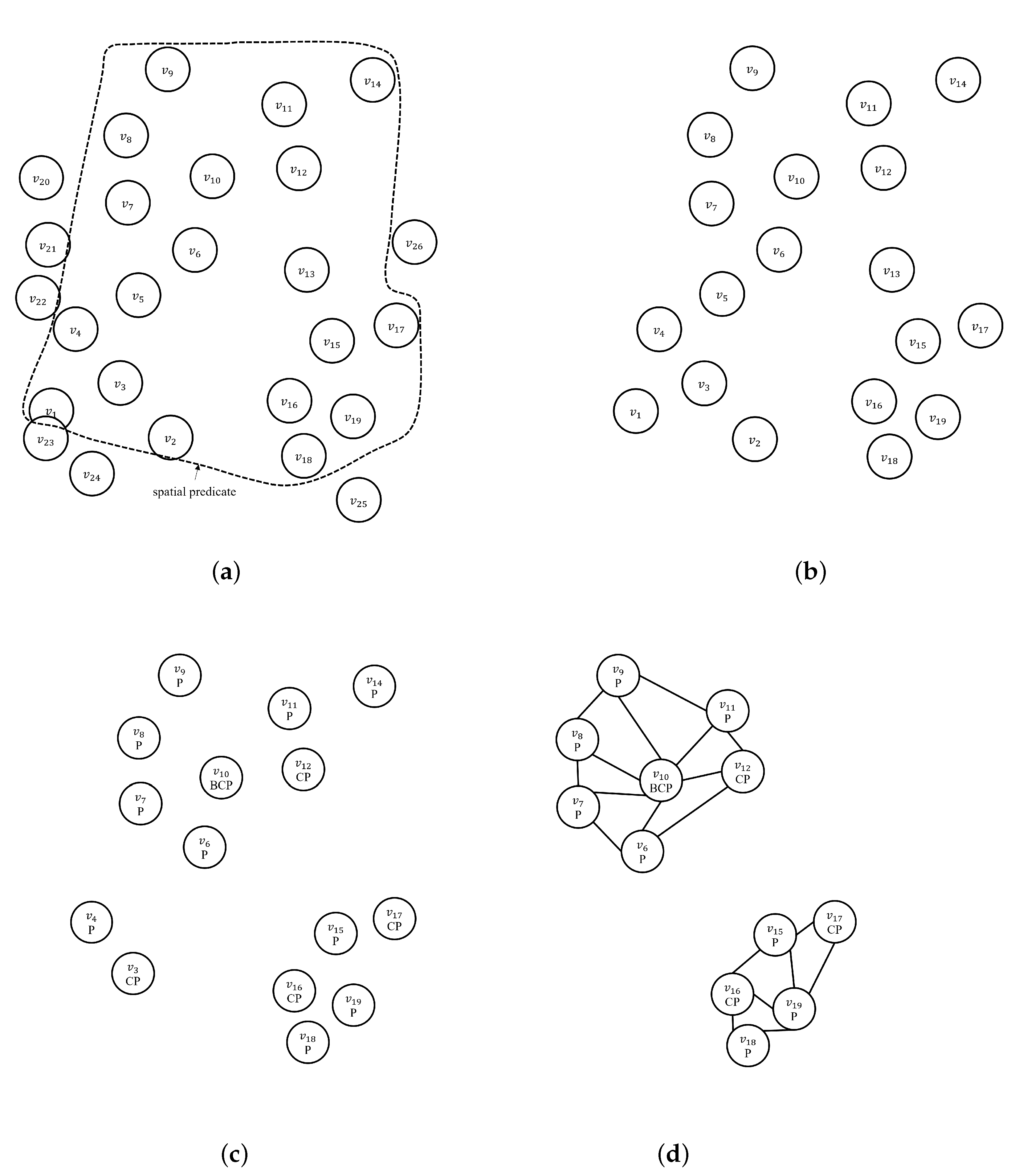
Figure 4.
An example of ClusterFirst DBSCAN. (a) after constructNNGGraph (k = 5); (b) after density clustering; (c) after deepSelection (dp = ‘person’); (d) after re-density clustering.
Figure 4.
An example of ClusterFirst DBSCAN. (a) after constructNNGGraph (k = 5); (b) after density clustering; (c) after deepSelection (dp = ‘person’); (d) after re-density clustering.
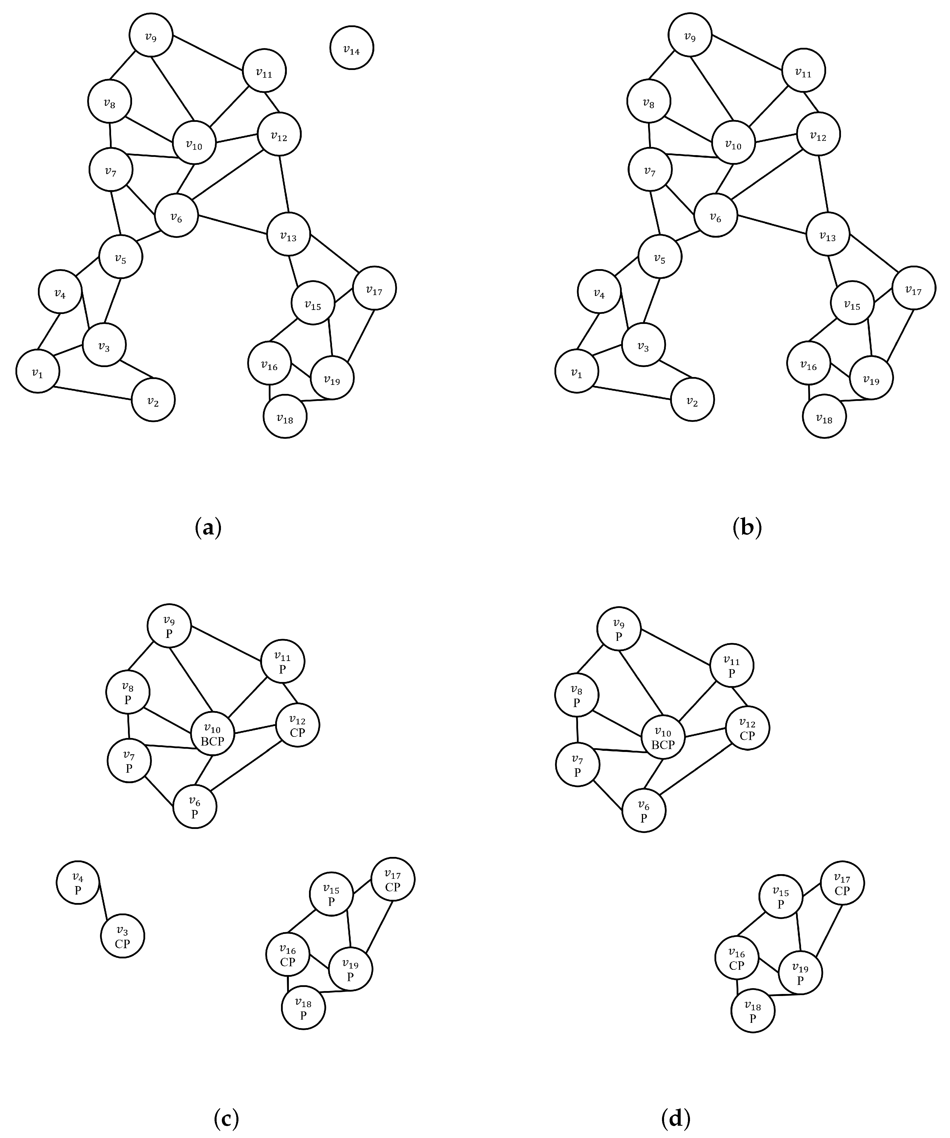
Figure 5.
An example of DeepDBSCAN. (a) after constructNNGGraph (k = 5); (b) after deepSelection, while traversing core vertices with the largest number of neighbors; (c) adjusted number of neighbors when neighbor vertexes or core vertexes dropped; (d) after density clustering.
Figure 5.
An example of DeepDBSCAN. (a) after constructNNGGraph (k = 5); (b) after deepSelection, while traversing core vertices with the largest number of neighbors; (c) adjusted number of neighbors when neighbor vertexes or core vertexes dropped; (d) after density clustering.

Figure 6.
Experimental layout.

Figure 7.
Effect of the data size. (a–c) number of object detections when minpts 9 to 21; (d–f) The time cost of each object detection model when minpts 9 to 21.
Figure 7.
Effect of the data size. (a–c) number of object detections when minpts 9 to 21; (d–f) The time cost of each object detection model when minpts 9 to 21.
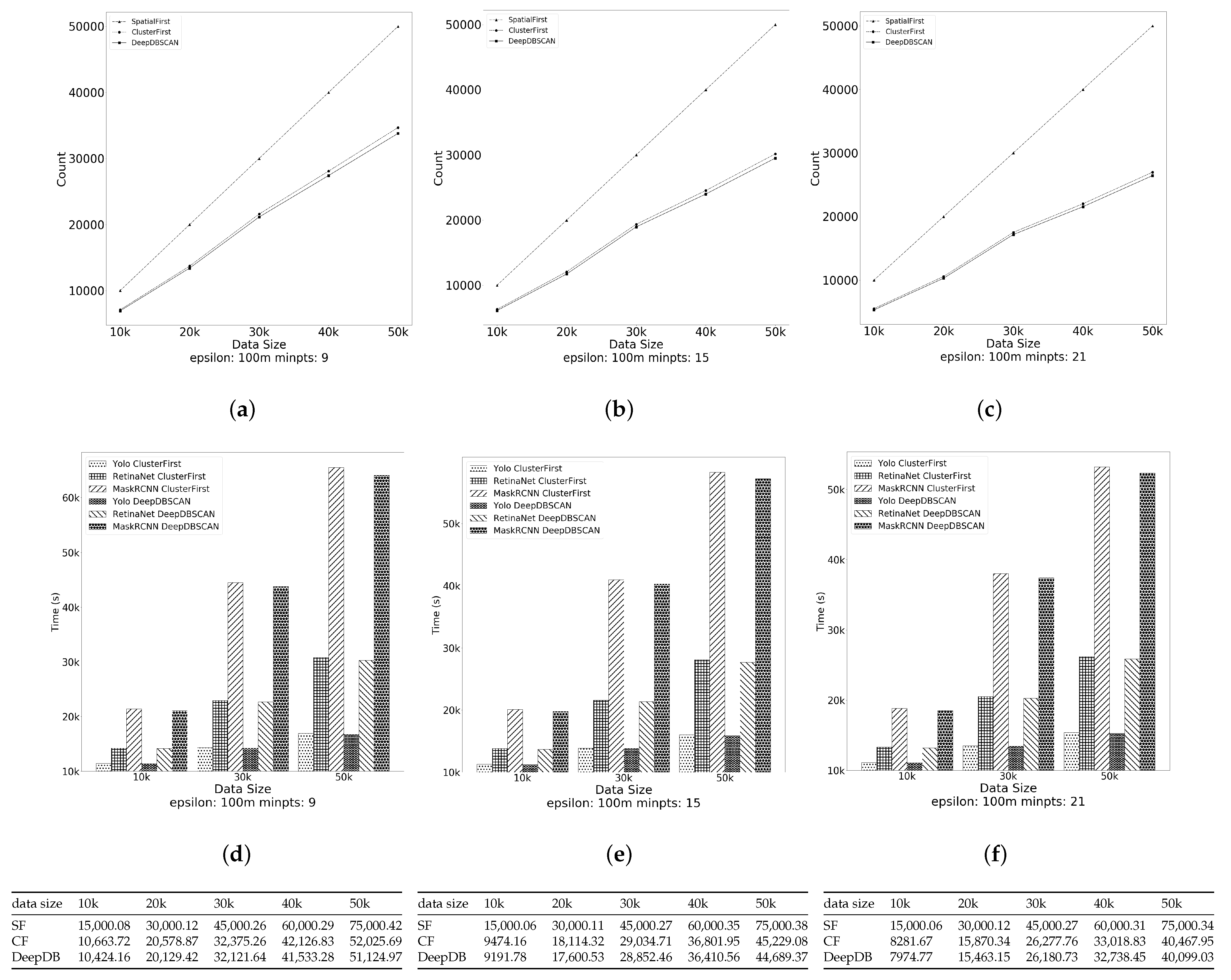
Figure 8.
Effect of the radius. (a–c) number of object detections when minpts 9 to 21; (d–f) The time cost of each object detection model when minpts 9 to 21.
Figure 8.
Effect of the radius. (a–c) number of object detections when minpts 9 to 21; (d–f) The time cost of each object detection model when minpts 9 to 21.
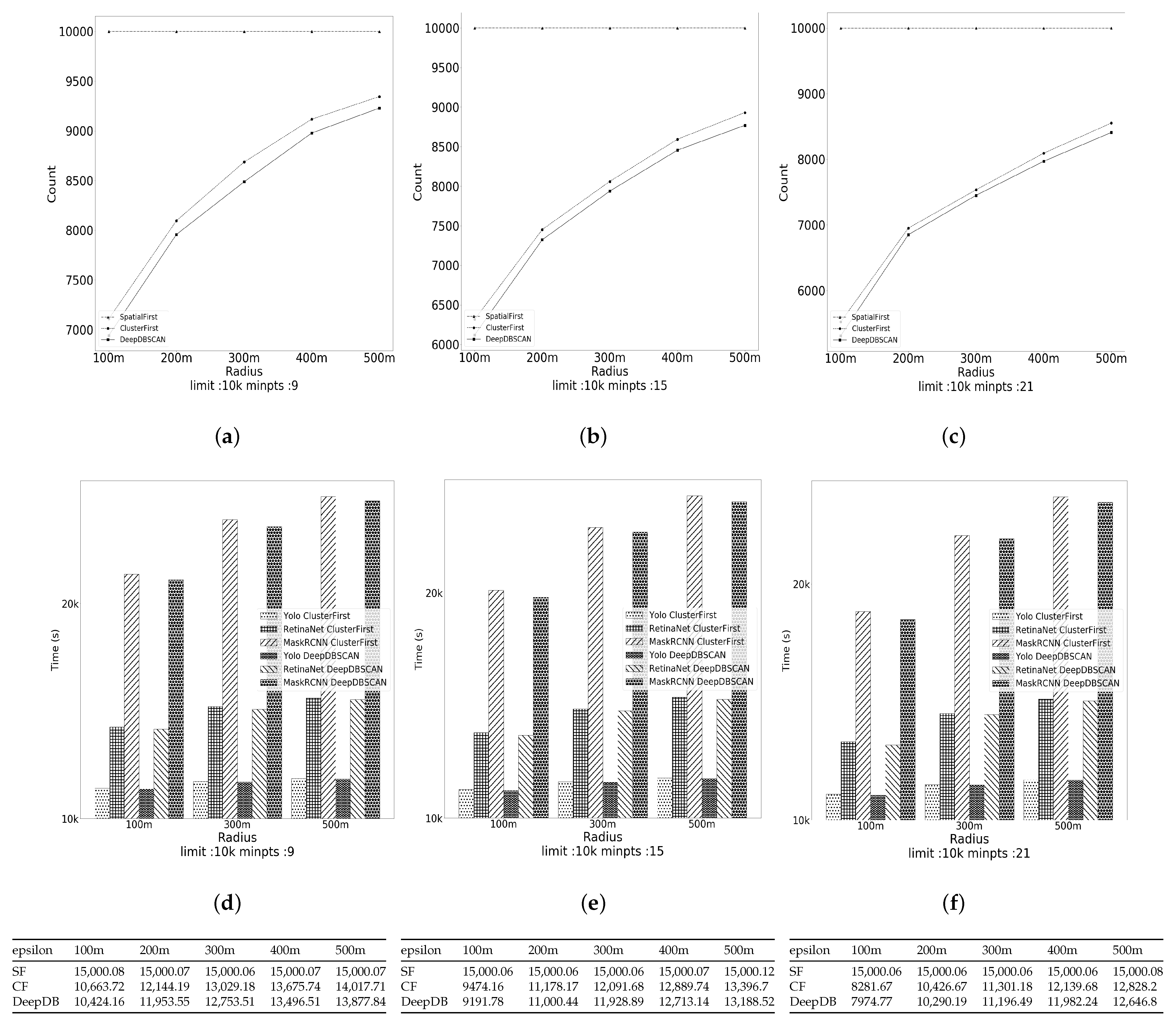
Figure 9.
Effect of the minimum number of points. (a–c) number of object detections when epsilon 100 m to 500 m; (d–f) The time cost of each object detection model when epsilon 100 m to 500 m.
Figure 9.
Effect of the minimum number of points. (a–c) number of object detections when epsilon 100 m to 500 m; (d–f) The time cost of each object detection model when epsilon 100 m to 500 m.
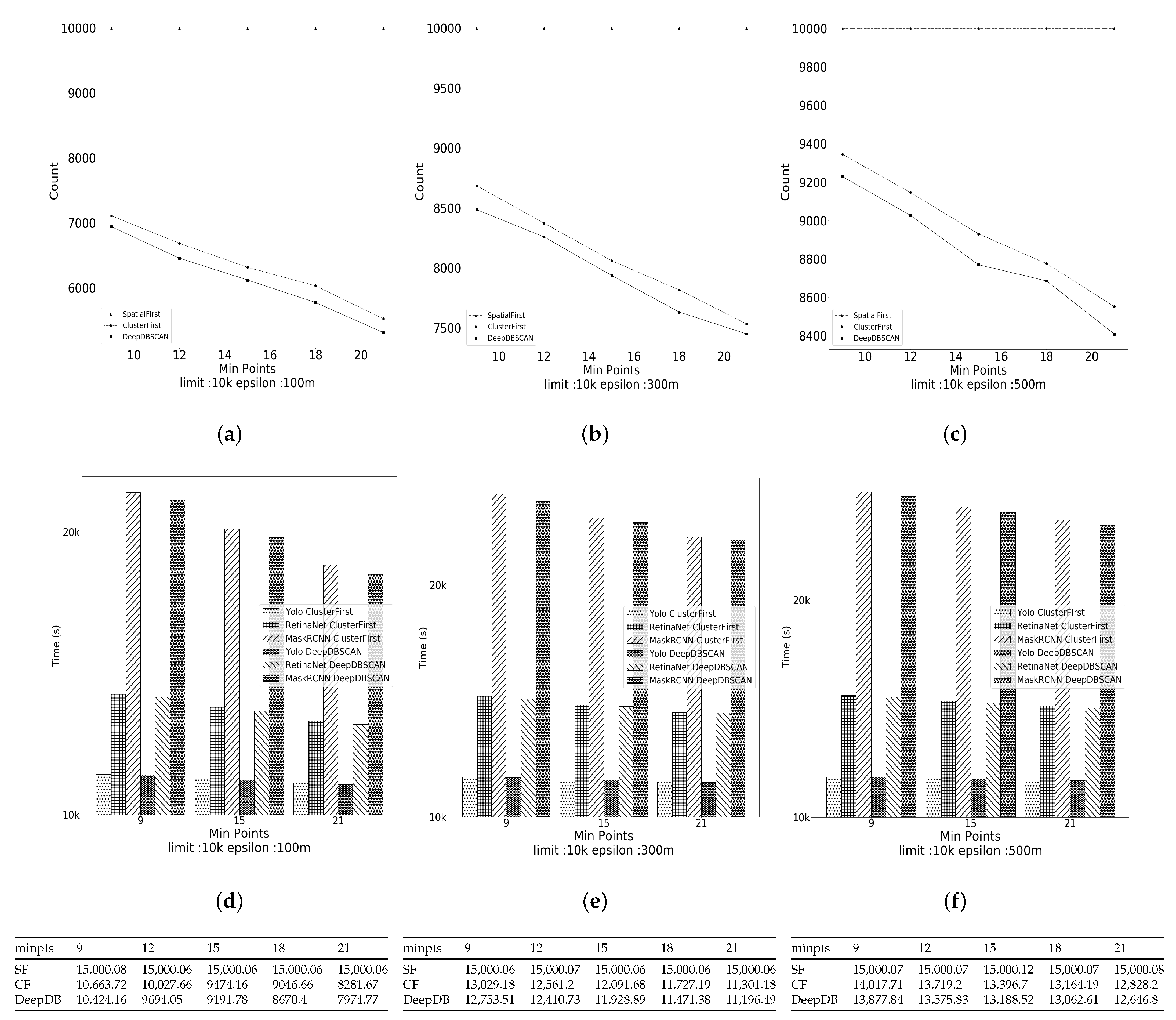
Figure 10.
Experimental data samples and clustering results.

Table 1.
Notations and description.
| Notation | Description |
|---|---|
| P | Geo-tagged photos |
| Nearest neighbor graph | |
| C | A set of clusters |
| V | A set of vertices for geo-tagged photos |
| Spatial predicate | |
| Deep content-based predicate | |
| k | Minimum number of points |
| Threshold of the radius for neighbors |
Table 2.
Sorted .
| vertex | isCore | isNoise | neighbors |
|---|---|---|---|
| T | F | {, , , , , , } | |
| T | F | {, , , , , } | |
| T | F | {, , , , } | |
| T | F | {, , , , } | |
| T | F | {, , , , } | |
| F | F | {, , , , } | |
| T | F | {, , , , } | |
| T | F | {, , , , } | |
| T | F | {, , , , } | |
| F | F | {, , , } | |
| F | F | {, , , } | |
| F | F | {, , , } | |
| F | F | {, , , } | |
| F | F | {, , , } | |
| F | F | {, , , } | |
| F | F | {, , } | |
| F | F | {, , } | |
| F | F | {, , } | |
| F | F | {} |
Table 3.
NNG after the algorithm ends.
| vertex | isCore | isNoise | neighbors |
|---|---|---|---|
| T | F | {, , , , , , } | |
| F | F | {, , , } | |
| F | F | {, , , } | |
| F | T | {} | |
| F | F | {, , , } | |
| F | F | {, , , } | |
| F | T | {} | |
| F | F | {, , , } | |
| T | F | {, , , , } | |
| F | F | {, , , } | |
| F | F | {, , , } | |
| F | F | {, , , } | |
| F | F | {, , , } | |
| F | F | {, , , } | |
| F | F | {, , } | |
| F | F | {, , } | |
| F | F | {, , } | |
| F | F | {, , } | |
| F | T | {} |
Publisher’s Note: MDPI stays neutral with regard to jurisdictional claims in published maps and institutional affiliations. |
© 2021 by the authors. Licensee MDPI, Basel, Switzerland. This article is an open access article distributed under the terms and conditions of the Creative Commons Attribution (CC BY) license (https://creativecommons.org/licenses/by/4.0/).
Share and Cite
MDPI and ACS Style
Park, J.Y.; Ryu, D.J.; Nam, K.W.; Jang, I.; Jang, M.; Lee, Y. DeepDBSCAN: Deep Density-Based Clustering for Geo-Tagged Photos. ISPRS Int. J. Geo-Inf. 2021, 10, 548. https://doi.org/10.3390/ijgi10080548
AMA Style
Park JY, Ryu DJ, Nam KW, Jang I, Jang M, Lee Y. DeepDBSCAN: Deep Density-Based Clustering for Geo-Tagged Photos. ISPRS International Journal of Geo-Information. 2021; 10(8):548. https://doi.org/10.3390/ijgi10080548
Chicago/Turabian StylePark, Jang You, Dong June Ryu, Kwang Woo Nam, Insung Jang, Minseok Jang, and Yonsik Lee. 2021. "DeepDBSCAN: Deep Density-Based Clustering for Geo-Tagged Photos" ISPRS International Journal of Geo-Information 10, no. 8: 548. https://doi.org/10.3390/ijgi10080548
Note that from the first issue of 2016, this journal uses article numbers instead of page numbers. See further details here.