1. Introduction
Accurate information extraction from historical maps through vectorization is a challenging task due to the limited graphical quality of these maps, overlapping features, and lack of metadata, despite occasionally available archival data [
1]. Geoinformation generated from historical maps provides very useful input for the reconstruction of past landscape characteristics. This information offers unique geographical and political insights for historians and archaeologists to analyze the past and present existence of the social and economic interactions of communities and their historical legacies [
2,
3]. Moreover, by going back to the previous centuries with the aid of historical maps, land changes in the long run could be modeled. This information could be integrated into geographic information systems (GISs) to be used in various applications such as detailed historical analysis, urban and city planning, and disaster management studies. Large collections of historical map and plan archives could be used to create information on the changes which occurred in many historic towns and cities across the world [
4,
5].
Most of the accessible historical maps are digitally available only as scanned images; therefore, it is not possible to conduct quantitative and geometrical analysis from these maps without further processing [
6]. However, multi-date historical maps or integrated usage of historical maps, aerial photographs, and satellite images can be used to extract geographic features such as the spatial distribution of settlements and transportation infrastructures. Logistic information, and more specifically roads, are of central importance for long-term multimodal transport network reconstructions and traffic simulations. Historical maps, especially military maps with their special focus on transport infrastructures, are the best sources to extract valuable logistic data for past transport features, due to the fact that these maps are produced to be used in troop movements in possible military conflicts or planned invasions. During World War II, the German General Staff’s Department of Wartime Map and Survey Service (
Generalstab des Heeres, Abteilung für Kriegskarten und Vermessungswesen) had around 15,000 military and civil personnel. This unit produced in the relatively short period of the war an astonishing number of maps, totaling approximately 1.3 billion maps [
7]. The
Deutsche Heereskarte 1:200,000 Türkei (DHK 200 Turkey) series was a part of this massive military cartographical effort to be used during WWII. The DHK 200 Turkey was produced by the Main Survey Department (
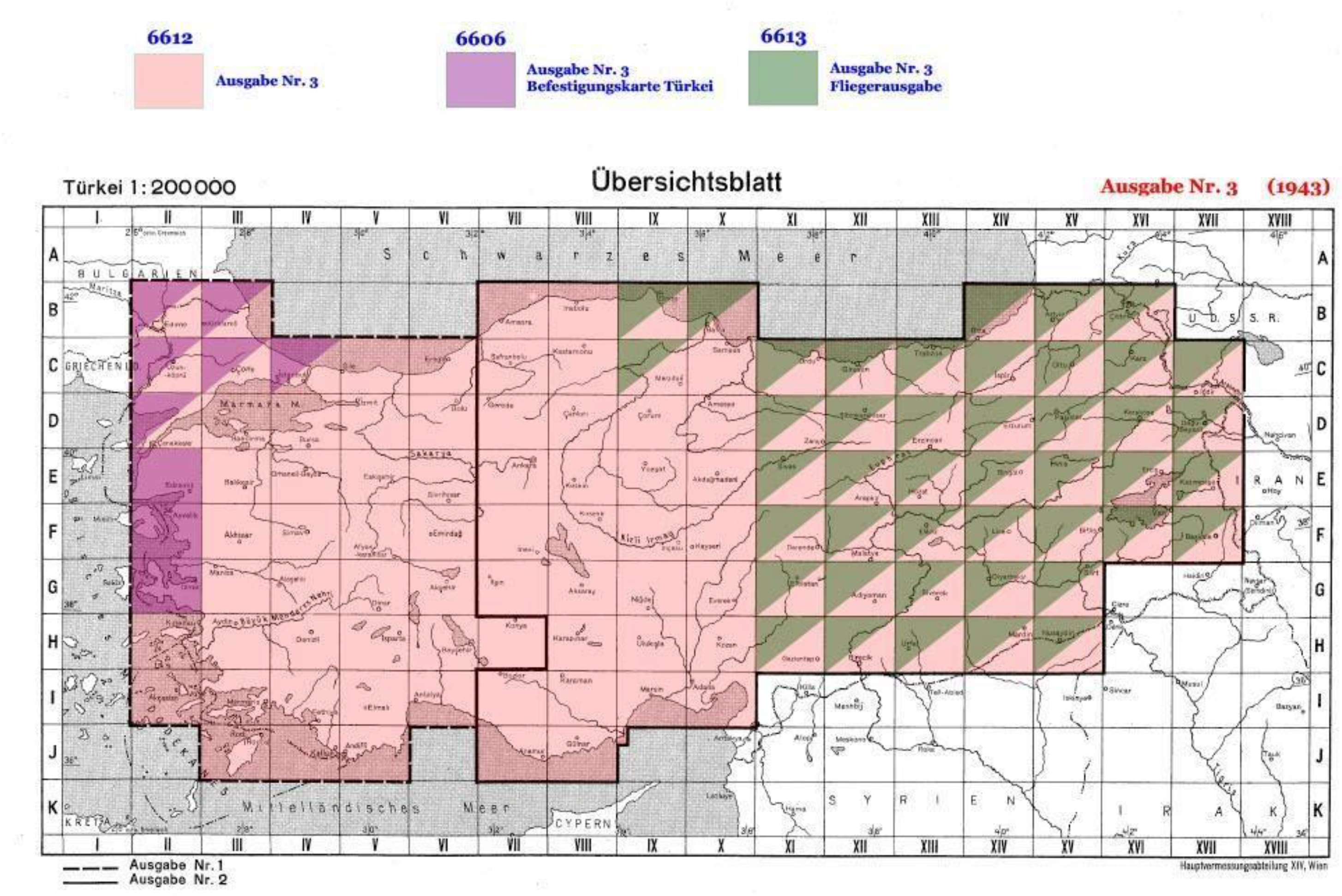
Hauptvermessungsabteilung) XIV in Vienna in 1942–1943. It exists in six different versions with around 400 sheets, covering almost the whole of Turkey. Several state and university libraries have copies of the DHK 200 Turkey and made them available online. To our knowledge, the McMaster University Library has the largest, albeit incomplete, available online collection (
http://digitalarchive.mcmaster.ca/islandora/object/macrepo%3A82339, accessed on 19 July 2021). We acquired the complete 3rd special issue, version 6612 from the Austrian Federal Office of Metrology and Surveying’s Cartography Department/Historical Map Archive in Vienna, which has the archives of the Main Survey Department XIV, the producer of the DHK 200 Turkey, due to the institutional continuity (see
Figure 1). The 3rd special issue has a total of 115 sheets. Some of these are divided into two parts (east and west), and there are a total of 138 images.
Vectorization of historical maps and aerial photographs has been conducted mainly through the on-screen digitization technique, which is time-consuming and labor-intensive [
4,
8,
9]. Manual digitization has still been widely used for reliable labeled data preparation for use in the learning process of artificial intelligence-based approaches. It took in total 1250 h to digitize and label 300,000 km of roads, including more than 64,000 segments from the
Generalkarte, another military map [
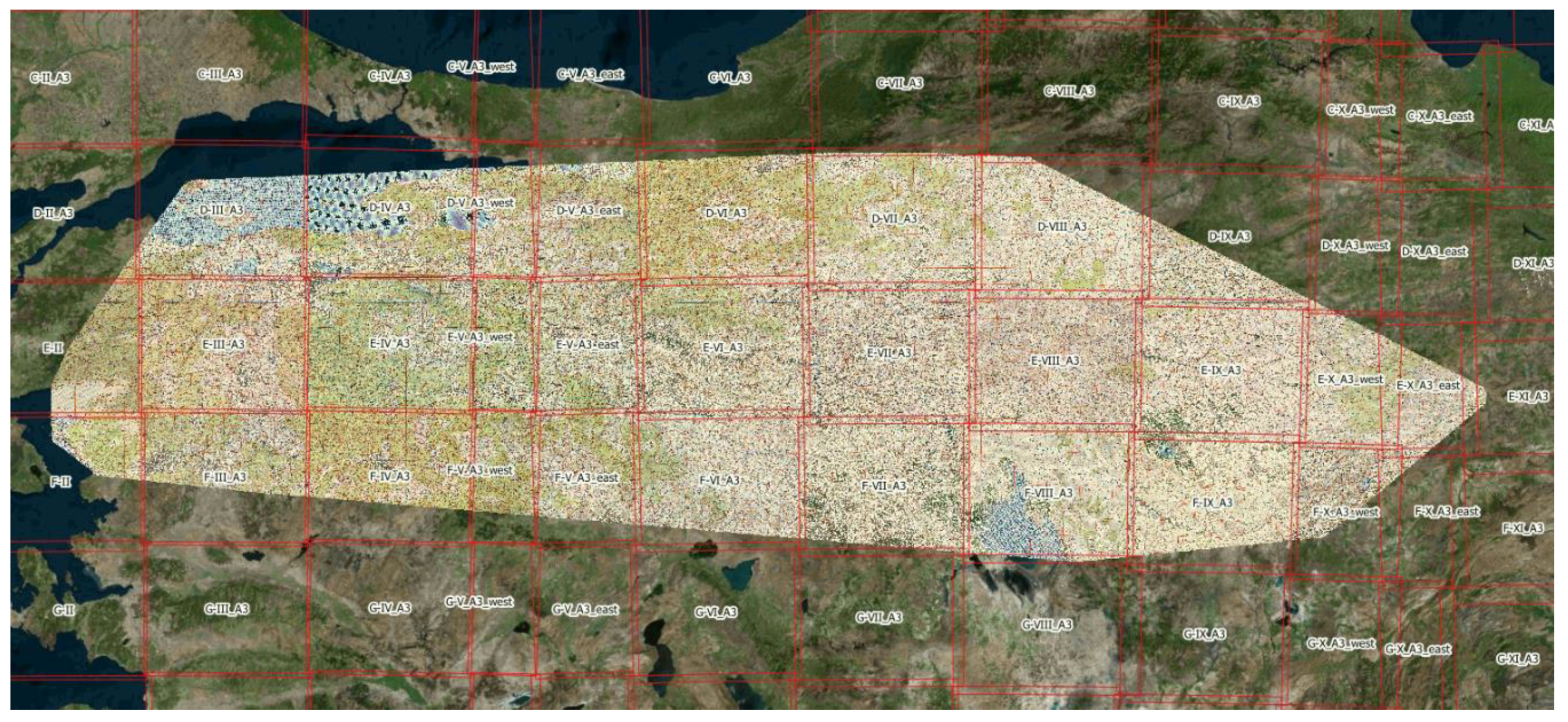
9]. For the digitization of DHK 200 Turkey, we spent around 1500 h extracting roads for a total of 85 images out of 138. We used the original projection system of the map, EPSG: 28405—Pulkovo 1942/Gauss–Kruger zones 5–8, and coordinates written on the borders of individual sheets.
With the increased availability of aerial photographs and satellite images, deep learning methods have become an important research topic in remote sensing for the extraction of geographic information, specifically by applying object detection, classification, and segmentation tasks [
10,
11,
12]. Cheng et al. [
13] provided a comprehensive review on the image scene classification task and described the details of autoencoder-based, convolutional neural network (CNN)-based, and generative adversarial network (GAN)-based image scene classification methods. Yuan et al. [
14] conducted a complete review for the semantic segmentation of remotely sensed images. In particular, they explained the CNN architectures used in semantic segmentation such as U-Net, SegNet, and DeepLab. Moreover, deep learning-based methods have started to be implemented in historical map-related tasks recently [
2,
6,
9,
15].
Andrade and Fernandes [
2] proposed a conditional generative adversarial network-based architecture to synthesize satellite images from historical maps that combined the texture information from the input data and reproduced a better visual output of a synthesized satellite image.
Saeedimoghaddam and Stepinski [
15] used Inception-ResNet v2 architecture based faster region-based deep convolutional neural network (RCNN) method pre-trained on the Microsoft COCO dataset to determine the road intersections of single-line and double-line road symbols from the United States Geological Survey (USGS) maps by considering this as an object detection problem. They found better precision and recall values for double-line road symbols compared with single-line road symbols. Their F1 scores were 0.8 and 0.86 for single- and double-line road symbols, respectively. Their outputs were bounding boxes, and in some cases, the detected boxes were bigger than the ground truth boxes, based on analysis of the figures in their article. However, there was no specific information on the intersection of union (IoU) metrics to quantitatively analyze the match of the geometry between the ground truth and the model’s output. It is essential to provide precision, recall, and F1 scores as well as IoU metric values to better quantify the performance of a proposed approach and conduct benchmark analysis among different research outcomes.
Uhl et al. [
6] proposed a weakly supervised CNN-based framework for the extraction of buildings and urban areas from the USGS historical topographic maps published between 1893 and 1954. They compared the results of the VGGNet-16, LeNet, and AlexNet architectures, and the best classification accuracy results were obtained with VGGNet-16, whereas the lowest accuracy was obtained with the shallow LeNet architecture. Afterward, they implemented semantic segmentation in VGGNet-16.
Chiang et al. [
3] applied deep learning-based approaches for the recognition of railroads from 1:24,000 scale USGS historical topographic maps. They manually created the one-pixel-wide ground truth data by digitizing railroad centerlines, applying buffers to both sides, and finally making three-pixel-wide railroad representations. They implemented three different fully convolutional networks (FCNs) with VGG16, GoogLeNet, and a residual network (ResNet) with ImageNet pretrained weights. The best IoU value obtained was 23.09% with the FCN-ResNet architecture due to the lack of training data and the limited ability of the applied models to detect small objects. They also used a pretrained pyramid scene parsing network (PSPNet) on PASCAL VOC 2012, and their best IoU obtained was 29.04% with large-sized training data and a shallow layer. Their best performance of 62.22% for the IoU value was obtained with the modified PSPNet with skip connections in VGG16. There is no specific information on the recall, precision, or F-measure values.
Can et al. [
9] identified seven different road types from the
Generalkarte historical map series using CNN-based classifiers, with an IoU value of around 0.45 and a pixel-wise accuracy of 0.93. In general, the precision values of different road types were lower than the recall values. The highest F-measure values were obtained for
Karrenweg and
Erhaltener Fahrweg road types with values of 0.5321 and 0.5336, respectively, using the U-Net architecture. On the other hand, the F-measure values of other road types were between 0.1022 and 0.2234, and the authors emphasized the importance of having more training data for the remaining five road types.
This study proposes a novel, end-to-end deep learning-based framework for the automatic detection of different road types from the historical DHK 200 Turkey maps. The end results achieving superior performance compared with similar studies that exist in the literature show that the adopted approach is capable of providing rich information that can be utilized by end users in many ways. The geoinformation injection into prediction maps allows us to further analyze and conduct spatial analysis of the features extracted from the historical maps and facilitates the integration of output predictions into a GIS environment.
3. Methodological Approach
3.1. Implementation Details
Both the training and subsequent inference phases of the DNN were implemented in the PyTorch (1.14.0) deep learning framework using the Python (3.8) programming language on a GeForce RTX 2080 Ti graphical processing unit. The semantic segmentation task was performed using segmentation-models-pytorch, a high-level library constructed on top of the PyTorch framework. The Albumentations library was used to deploy different augmentation techniques while feeding the data to the DNN model. As for geospatial data processing, QGIS and GDAL open-source software packages were used for the reprojection and rasterization steps and for the creation of smaller patches during the tiling process, respectively.
The task of pixel-wise classification is one of the most studied topics of the computer vision community, where the aim is to perform dense (pixel-wise) prediction on an input image according to a predefined class legend [
13]. Early work on deep learning-powered semantic segmentation mainly concentrated on CNNs to generate a dense prediction output. However, CNNs are not fully capable of producing high-quality dense predictions, as their last layer consists of a fully connected layer in which the final feature map is flattened. As was noticed later, flattening the feature map damages the output semantic understanding capacity considerably. To this end, nowadays, most semantic segmentation architectures follow the idea first coined in fully convolutional networks (FCNs) [
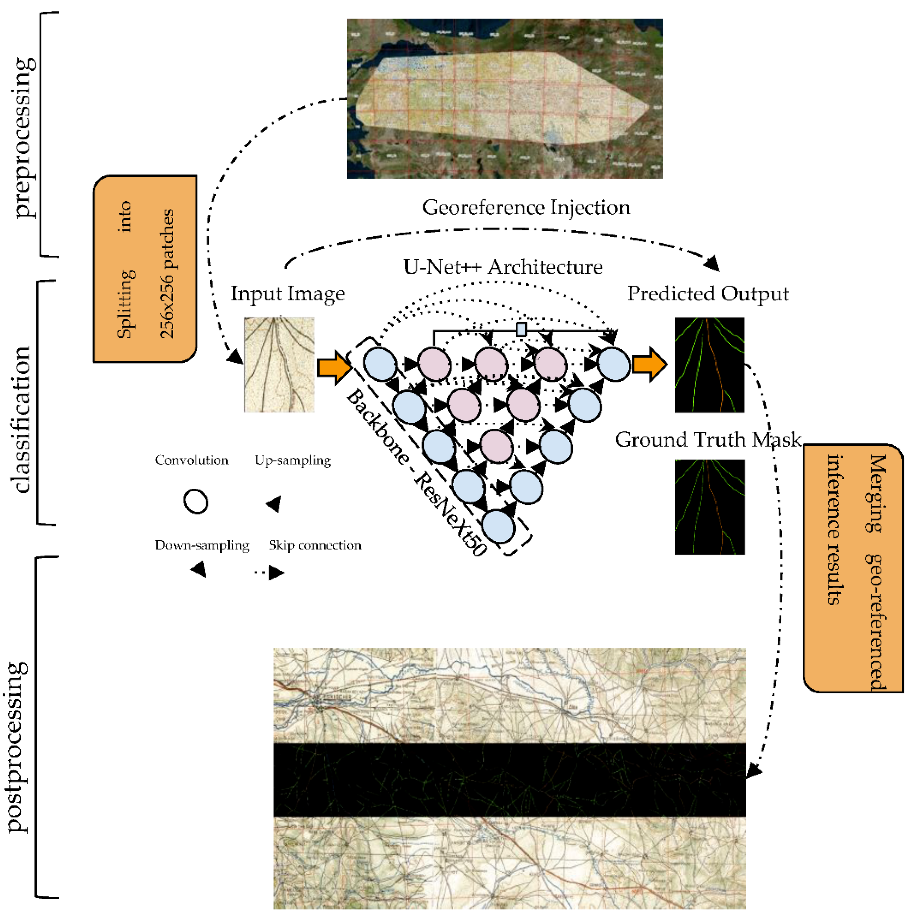
17]. To put it simply, the idea is to construct autoencoder-guided logic in which the input is passed through consecutive encoder and decoder blocks. The encoder block performs downsampling, resulting in latent space representation of the input data where the decoder block conversely mimics the encoder block to upsample the feature map back to the size of the input image. The other building block of the DNN-based semantic segmentation pipeline is CNNs. CNNs are particularly used in the encoder block of the semantic segmentation architecture to ease the feature extraction process. With the use of pretrained CNNs in the semantic segmentation architecture, it is possible to benefit from ImageNet pretrained weights, which is especially helpful for high-level feature extraction from the input despite the domain gap that emerges as a consequence of the natural images used to train the ImageNet. The overall workflow is illustrated in
Figure 8. Here, georeference injection denotes a post-training phase where the georeference information from the input map is injected into each corresponding ground truth mask to further constitute the georeferenced tile.
In light of the previous superior performance achieved, U-Net++ [
18] and ResneXt50_32x4d [
19] architectures were adopted in this study to produce segmentation masks and perform feature extraction. U-Net++ architecture is the successor of U-Net, where the skip connections are revisited to alleviate the contextual gap between the features of the encoder and the decoder subnetworks. The goal lay in the assumption that optimization of the DNN model would be less challenging when the contextual similarity between the encoder and decoder subnetworks was promoted.
In general, U-Net++ diverges from U-Net in the following ways. The first difference is the use of convolution layers on skip connections, which tries to boost the contextual similarity among the feature maps. The approach to skip connections within the context of CNNs is coined in the ResNet architecture and helps to enhance the performance by easing the flow of the gradient through the DNN model. The second distinction arises from the introduced deep supervision method that allows for generating precise and fast pixel-wise classification maps either by taking the middle branches or choosing only one pixel-wise classification branch with the goal of DNN pruning [
18,
20].
As shown in
Figure 8, the selected layer depth in the U-Net++ architecture was five. The DNN model received an input with the shape of (256 × 256 × 3) and output a segmentation map with the shape of (256 × 256 × 6), with 6 being the number of classes. Pretrained ImageNet weights were adopted to ease the feature extraction process. Augmentation techniques were adopted to increase the dataset size artificially on the fly by performing basic image processing techniques such as flip, crop, Gaussian noise, perspective, brightness, gamma, sharpen, blur, and motion blur. This is an especially useful technique that enables the DNN model to generalize the test samples better. The DNN model was trained for 15 epochs, and optimization was performed using the Adam algorithm with a learning rate of 0.0001 and an epsilon of 10
−8. During the training phase, the F1 score was monitored to assess the performance of the DNN model. The quantification of the DNN model’s learnable parameters quality is represented by dice loss [
21], which is formulated as follows:
where
and
are either 0 or 1, denoting the pixel value of the prediction mask and the ground truth mask, respectively. Multiplying the value in the numerator by 2 helps to compensate for the double counts of the instances in the denominator. Furthermore, subtraction from 1 is performed to construct a loss function that is suitable for minimization. Dice loss turns the dice coefficient into a differentiable form, in which it can be used as a loss function. This is especially useful in segmentation tasks where the overlapping of two segments needs to be considered in calculating the accuracy. In addition, considering the class unbalance issue in our dataset, it facilitates the learning of the underrepresented classes.
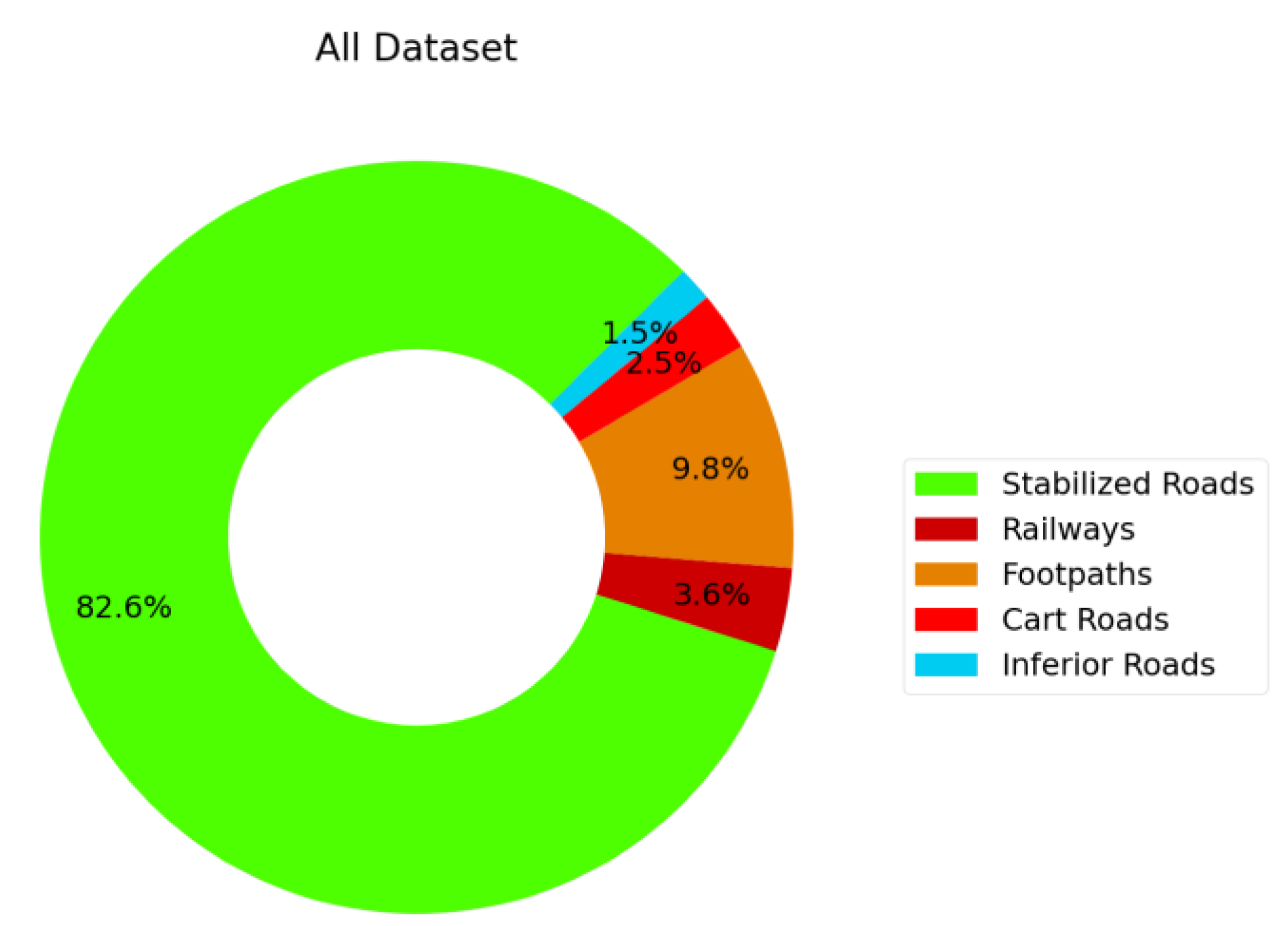
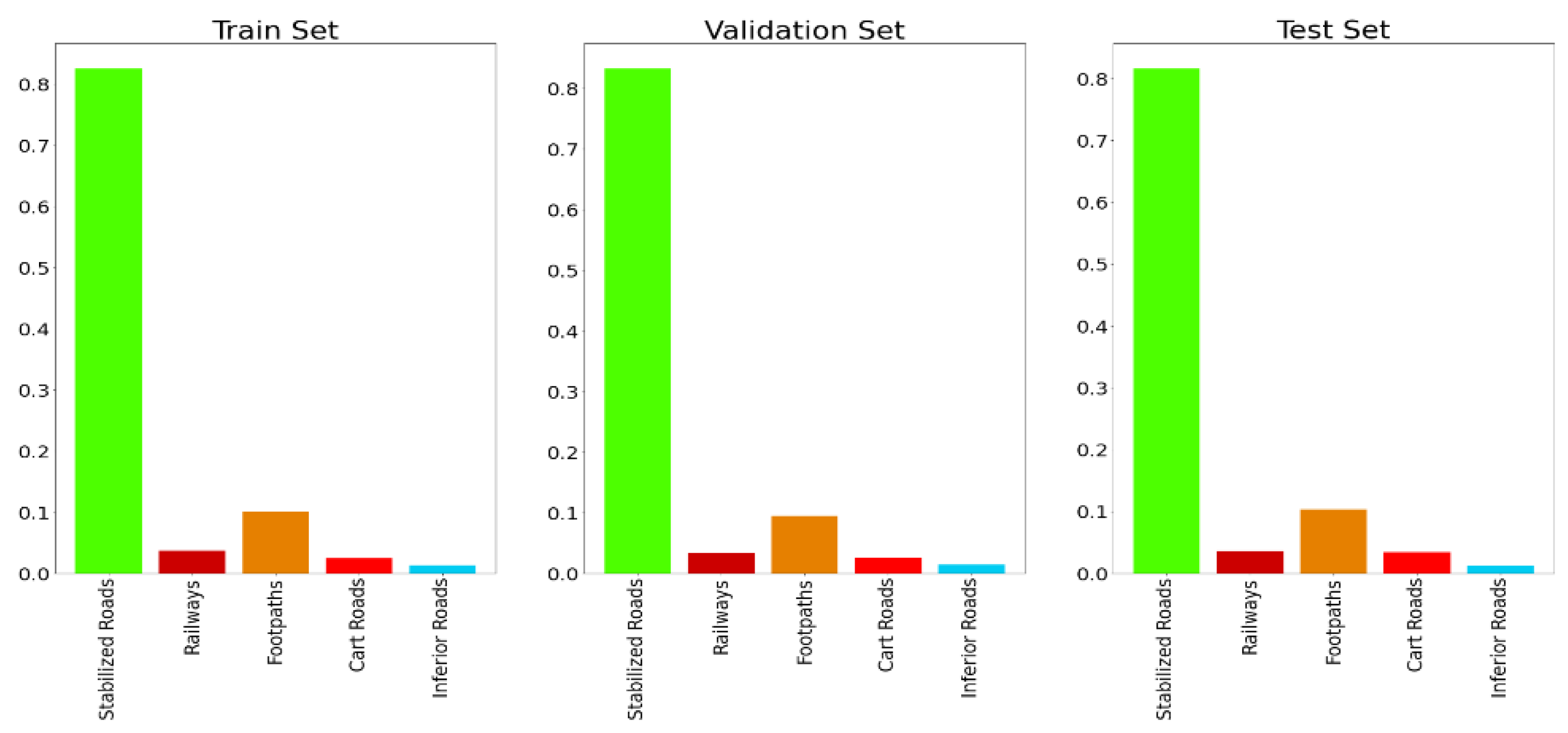
As was previously mentioned, the dataset used in this study suffered from the class imbalance problem. This is a challenging problem in DNN model training, and it should be eliminated as much as possible. In this study, to cope with this phenomenon, a sampling method was performed simply by oversampling the underrepresented road types and undersampling the overrepresented road types. More specifically, this method was performed as follows. First, all ground truth masks in the training and validation sets were quantified with an integer value by considering the number of distinct road types contained within. Second, the sample weights were calculated, and each sample was assigned with a weight value that indicated the importance of the sample by considering the number of road types it contained. Lastly, the number of samples was multiplied by the offset to expand the samples, and the sample weights were used as an input for the sampler function, which was responsible for forming image batches to feed to the DNN model. From the practical implementation point of view, sklearn’s compute_sample_weight function was used for the weight calculation. The calculated weights were given to the PyTorch DataLoader class as a sampler instance, which oversampled or under sampled each sample in the training set. The weights were calculated by taking the class-type occurrences in each training set sample into account. Simply, the samples (ground truth mask) consisting of high numbers of classes were given higher weights, indicating the sample’s importance.
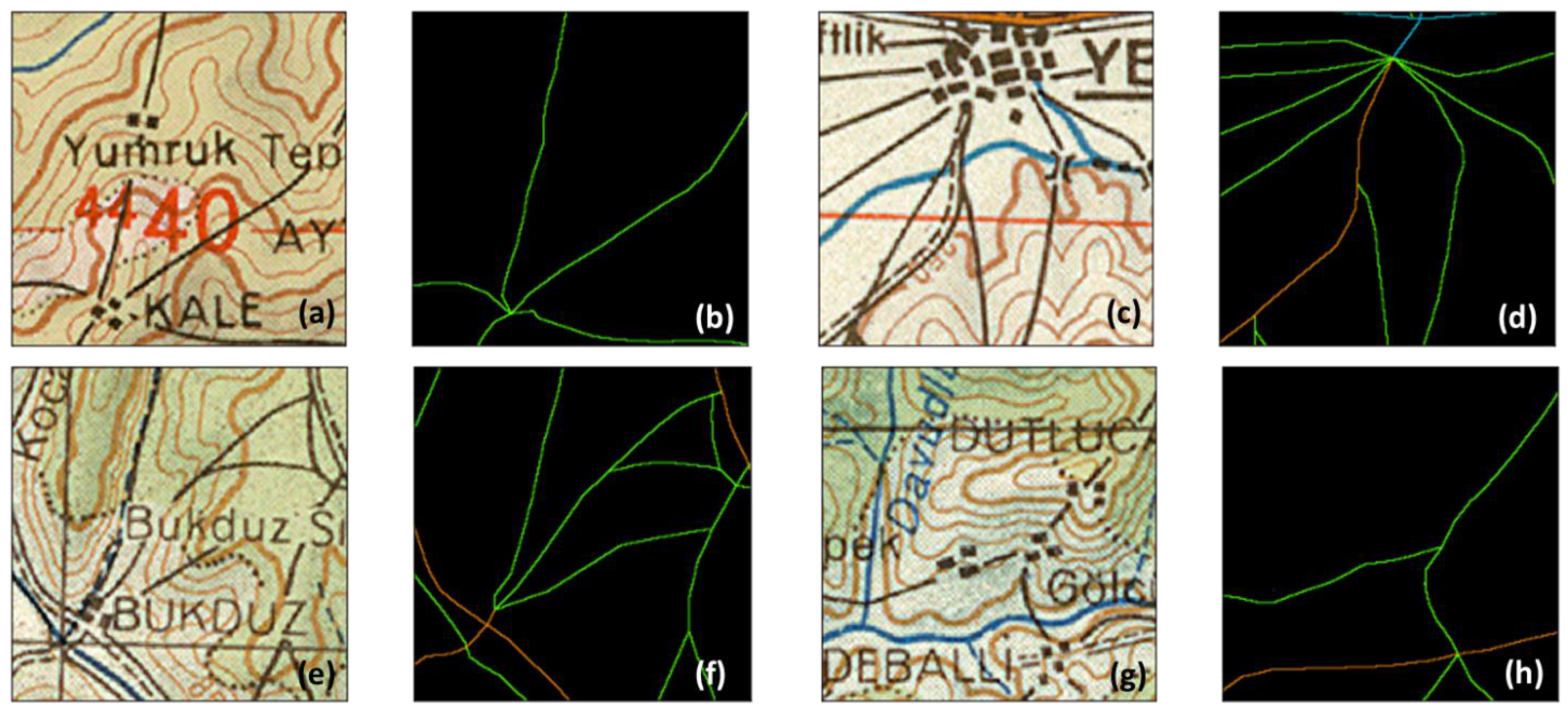
As can be easily drawn from
Figure 4, in some cases where the road was occluded by map markers, the ground truth mask did not provide a full and precise expression of the road types in the map. Although the road interfered with the map markers, it is indisputable that there were road networks that existed on the occluded part of the map. The evaluation metrics performed statistical analysis by taking the difference between the ground truth mask and the produced inference result into consideration. Thus, this phenomenon would severely mislead the end user by yielding incoherent inference results. It is crucial to cope with this aliasing effect to have a viable understanding of the performance of the DNN model. To this end, as a side experiment, we hand-picked the road networks relatively less occluded by map markers out of the test set samples and performed an inference on the DNN model that was trained on the original dataset with a high number of occluded samples.
3.2. Evaluation Metrics
Both for the sake of comparability with similar studies and to adequately assess the performance of the classifier, it was vital to employ descriptive evaluation metrics that were capable of identifying and capturing the ability of the classifier. Apart from providing visual test results, the performance of all experimental set-ups conducted in this study were assessed with widely used evaluation criteria: the F1 score, precision, recall, IoU, and confusion matrix. This subsection aims to describe these criteria briefly.
3.2.1. Precision, Recall, and F1 Scores
Precision and recall scores are the building blocks of several popular evaluation metrics, as they help to describe the classifier’s performance in a broad perspective in terms of exactness and sensitivity, respectively. The F1 score, on the other hand, is a widely adopted evaluation metric for classification tasks, as it provides a descriptive identification of the classifier by combining both the precision and recall scores by computing their harmonic mean; that is to say, the F1 score expresses harmony, whereas unbalanced precision and recall scores are penalized. All scores described here take a value between 0 and 1, with 0 being the lowest and 1 being the highest. The precision, recall, F1 score, and accuracy are calculated as follows:
3.2.2. IoU Score
The intersection over union score, also called the Jaccard Index, is especially beneficial in the cases where one needs to numerically describe the overlapping level of the bounding boxes or segments in the case of pixel-wise classification or object detection in general. The IoU score ranges from 0 to 1, where 0 indicates no overlap and 1 indicates complete overlap in the instances. The higher the IoU score, the better the DNN model classifies the road types. The IoU score is described as
3.2.3. Confusion Matrix
Accuracy assessment is an integrated part of most mapping projects and calculation of the confusion matrix, and related metrics such as the overall, producer’s, and user’s accuracy and the kappa statistic are required to present quantitative value regarding the performance of the proposed approach [
22,
23]. The confusion matrix assists in expressing the classifiers’ ability to discriminate the classes. This indicator is especially useful for diagnosing the classifier in a class-wise fashion, not only for the inference phase but also for the pretraining phase.
4. Results and Discussions
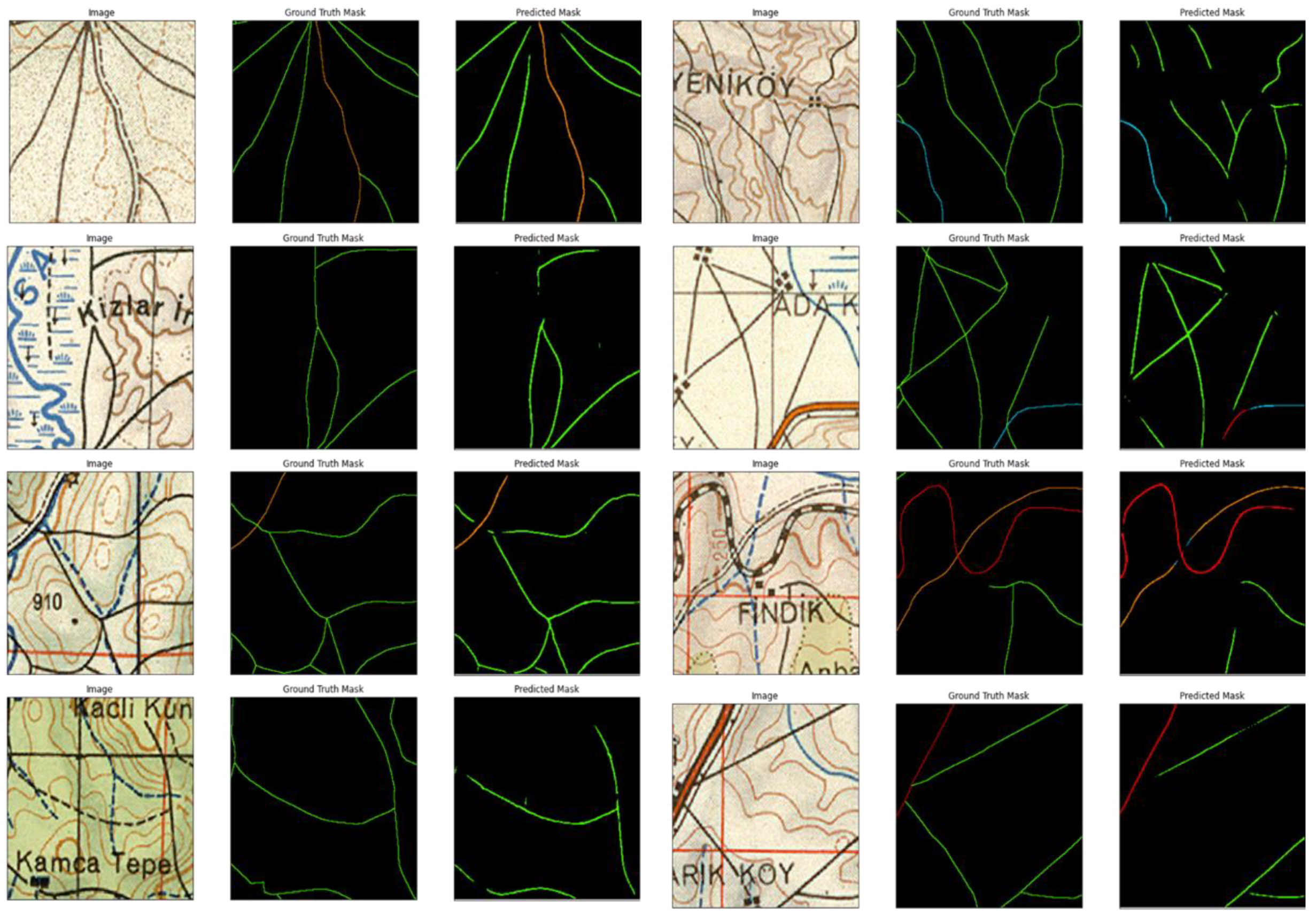
After the training phase, the test set instances were used to assess the model’s performance in both qualitative and quantitative ways by using the aforementioned evaluation metrics. As for the qualitative assessment, an end-to-end workflow was constructed where the input map patches were fed to the trained DNN to output georeferenced road-type masks. The test images and their prediction outputs generated by the DNN model are given in
Figure 9.
The quantitative results, on the other hand, were created by making use of the aforementioned and widely adopted evaluation metrics: the F1 score, precision, recall, IoU, and accuracy, where each metric exhibits a specific type of assessment criteria. The results are tabulated in
Table 1.
In light of the experimental results stated above, it is possible to conclude that the accuracy score provided optimistic value in capturing the performance of the classifier compared with the other evaluation metrics. Visual analysis of the results also verified this situation. As can be seen in
Figure 9, there were discrepancies between the ground truth and predicted road segments. More specially, the accuracy score seemed to be less capable of capturing the performance of the classifier. On the other hand, the remaining scores tended to be overly critical of the classifier’s performance. These discrepancies might be the result of the annotation strategy and precision in the annotations i.e., (1) the thickness of each road, (2) not having perfect overlap between the ground truth annotations and the road segments in the map, and (3) discontinuities of the road segments due to the annotations on the input historical maps.
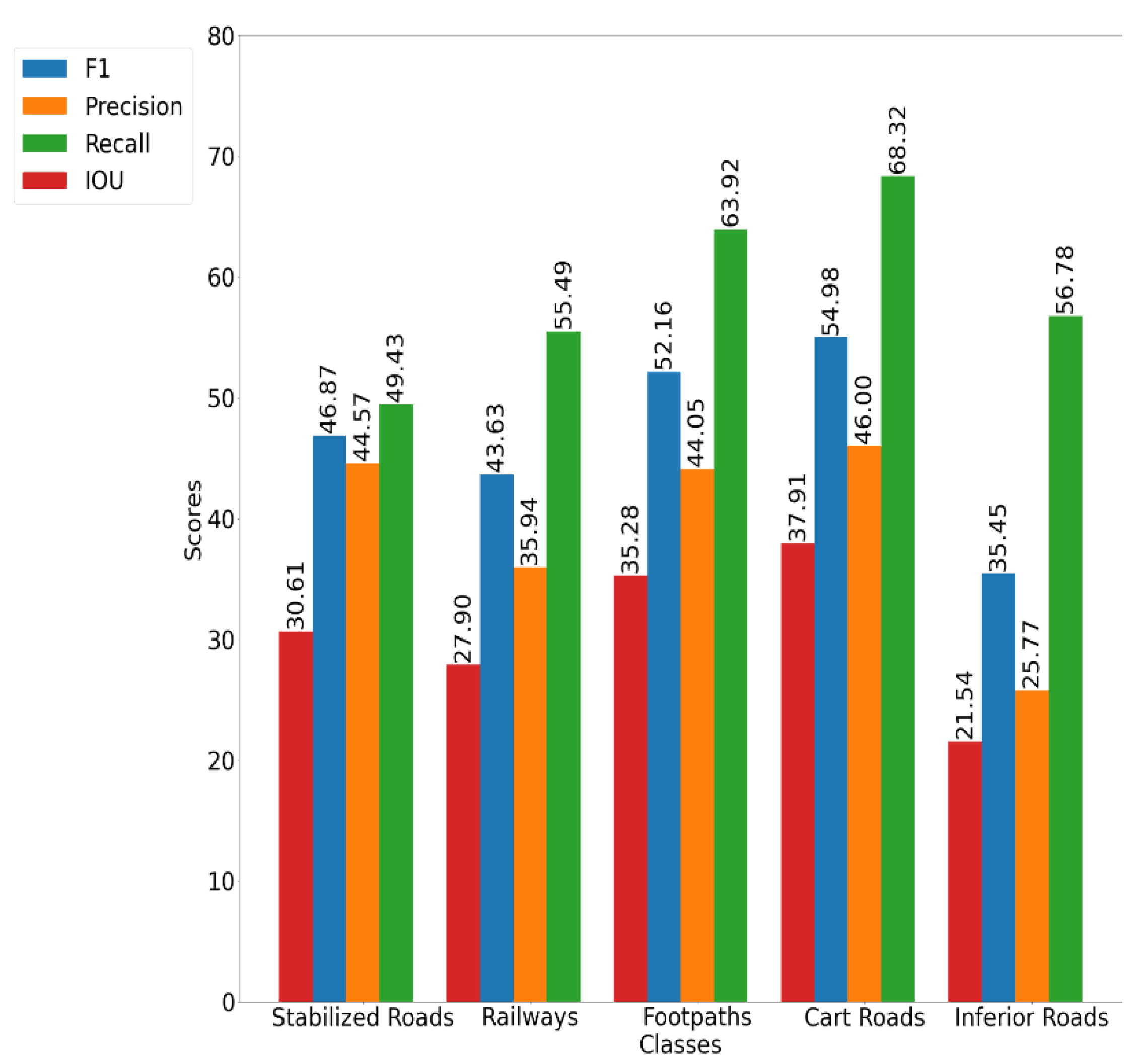
The class-wise F1, precision, recall, and IoU scores were calculated to have a better understanding of the performance of the DNN model in a class-wise manner.
From
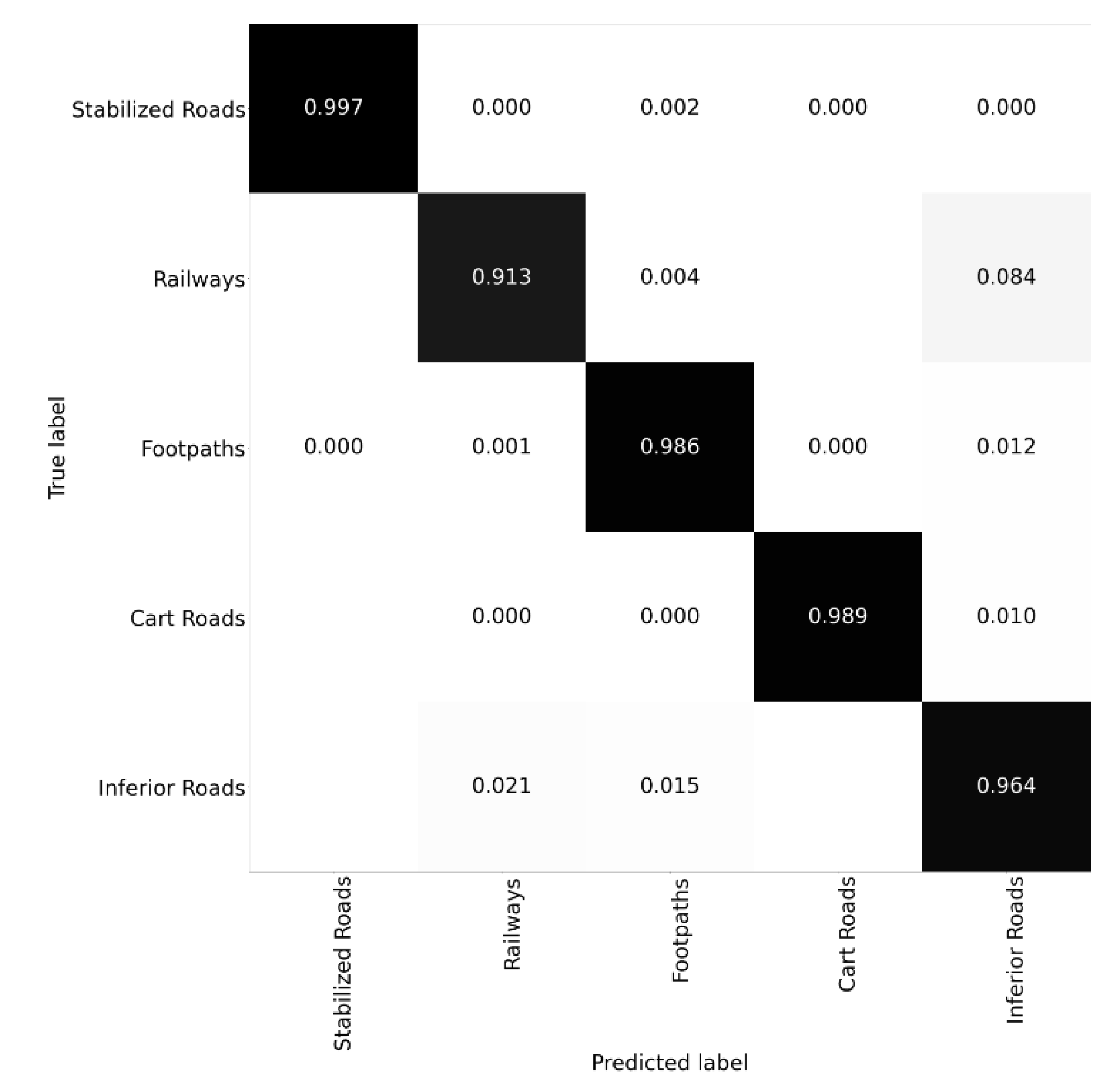
Figure 10, it is evident that the DNN model had trouble classifying and discriminating less-frequent and thus underrepresented classes. Further diagnosing the capability of the DNN model was realized by calculating the confusion matrix, shown in
Figure 11. From this figure, it is possible to conclude that railways and inferior roads were the most confused among all classes.
In the normalized confusion matrix, each cell in the confusion matrix denotes how good the classifier is at classifying that class pair. Ideally, each cell in the left-to-right diagonal is expected to be one, which indicates “zero confusion”.
From the confusion matrix, it is possible to infer that the classifier constructed in this study seemed to be capable of classifying all of the classes in the dataset with approximately similar performance. The less-frequent road type, inferior roads, achieved a 96.4% score, while the most frequent one, stabilized roads, achieved a 99.7% score. This achievement was mainly due to the sampling method adopted in this study, which took the class occurrences into account.
A side experiment was conducted which was motivated by the observation that some road segments were not continuous and were occluded in the original map by some annotations or other symbols. These road instances were digitized as continuous segments in the ground truth data with the contribution of analyst experience. However, since the original input images did not include road-type features in these cases, the performance of the DNN model was severely affected. To analyze this effect, we created a subset from our test set in which we referred to a non-occluded test set. We argue that the curated non-occluded test set is representative of the original test, as it consisted of 300 test samples. The experimental results after hand-picking the problematic samples are tabulated in
Table 2. The results show that there was an interesting type of image–ground truth pair inconsistency case, where the human annotator annotated the occluded and thus unseen roads on the map.
The DNN model performed as expected, since it output the prediction map solely from the input map. However, this scenario led to a vast deformation in the quantitative assessment, since the evaluation metrics calculated the difference between the ground truth and the output. The results tabulated in
Table 2 point out that the DNN model’s performance heavily relied on the quality of the ground truth masks that the DNN model was trained on.
Automatizing the task of road extraction from historical maps still poses several challenges, with occlusion-caused challenges being one of them, which was also examined in this study. According to the results tabulated in
Table 1 and
Table 2, it is possible to conclude that curating a dataset for the supervised classification task requires extra attention.
Since there is no common benchmark dataset for the task of road classification from historical maps, comparing the evaluation results of similar studies, especially from the quantitative analysis perspective, would yield incoherent results. By open-sourcing the dataset curated in this study, we aim to propose a benchmark for researchers to further investigate. This, we believe, is the most effective way of pushing the boundaries of the task at hand, as happened with the ImageNet challenges, which have been acting as a testbed for deep learning approaches.
5. Conclusions
In this research, we proposed a CNN-based solution for the fast and automatic extraction of different road types from historical maps. Our proposed method can be directly applied to other geographical regions of the same maps. As was explained above, the vast series of the WWII German military maps use the same or very similar legends. Therefore, a cross-examination only within this map series would be a worthwhile exercise on its own.
Moreover, our results can be used as a base for the transfer learning used for historical maps from different data sources. Our results showed that the main challenge for the automatic vectorization of roads was those segments having annotations, causing discontinuities in the road paths.
The proposed approach could be implemented into different raster maps for the extraction of roads, specifically for those regions in which road vector data are not readily available.
Given that the inconsistency in the image–ground truth pair yielded lower accuracies, it is possible to conclude that relying on a pixel-wise and dense annotation strategy may not be the future of the classification models. Supervised classifiers might perform weakly in scenarios which are not explicitly and adequately covered and represented in the training set. To this end, it would be interesting to investigate semi-supervised or unsupervised classification schemes more to cope with the extreme and challenging scenarios that might occur.


