A Closed-Form Solution to Planar Feature-Based Registration of LiDAR Point Clouds

Abstract

Since pairwise registration is a necessary step for the seamless fusion of point clouds from neighboring stations, a closed-form solution to planar feature-based registration of LiDAR (Light Detection and Ranging) point clouds is proposed in this paper. Based on the Plücker coordinate-based representation of linear features in three-dimensional space, a quad tuple-based representation of planar features is introduced, which makes it possible to directly determine the difference between any two planar features. Dual quaternions are employed to represent spatial transformation and operations between dual quaternions and the quad tuple-based representation of planar features are given, with which an error norm is constructed. Based on L2-norm-minimization, detailed derivations of the proposed solution are explained step by step. Two experiments were designed in which simulated data and real data were both used to verify the correctness and the feasibility of the proposed solution. With the simulated data, the calculated registration results were consistent with the pre-established parameters, which verifies the correctness of the presented solution. With the real data, the calculated registration results were consistent with the results calculated by iterative methods. Conclusions can be drawn from the two experiments: (1) The proposed solution does not require any initial estimates of the unknown parameters in advance, which assures the stability and robustness of the solution; (2) Using dual quaternions to represent spatial transformation greatly reduces the additional constraints in the estimation process.

1. Introduction

With the fast development of Light Detection and Ranging (LiDAR) techniques and their successful application in three-dimensional data acquisition, point cloud registration has attracted significant attention for its role in the fusion of LiDAR point clouds from two neighboring stations. The essence of point cloud registration is to estimate the transformation parameters between the two neighboring stations, which is also known as spatial transformation. As is known, a spatial transformation can be explained as a rotation around the x, y, and z axes, a translation along the three axes, and a scale factor based on the centroid of the coordinate system.

Based on the different registration primitives used for the estimation of unknown transformation parameters, the available methods can be categorized into point feature-based methods [1,2], linear feature-based methods [3,4,5], planar feature-based methods [6,7,8], and hybrid feature-based methods [9,10,11]. Until now, point features are still the most popular and widely used registration primitives for simple mathematical expressions. However, affected by the characteristics of LiDAR technology, the extraction of point features from point clouds often has low accuracy without pre-established man-made reflectors. Except for point features, linear features are another popular registration primitive. Compared to point and linear features, the extraction of planar features from point clouds is more convenient and often has higher accuracy. However, fewer available methods use planar features as registration primitives; this may be due to the diverse mathematical expressions, which make it difficult for us to compare and determine the differences between two planar features.

Moreover, according to whether the initial approximate estimates of those unknown transformation parameters are needed in advance, the available registration methods can be divided into two categories: iterative methods [1,2,5,9,12] and closed-form methods [13,14,15,16]. Most available methods obtain the registration results by iterative computation; however, their disadvantages must be treated properly. First, the nonlinear registration model must be linearized before it can be calculated by computers, and the initial approximate estimates of those unknown parameters must be determined in advance to assist the linearization. Second, the number of iterations is closely related to the choice of those initial estimates; that is, when they are not close to the maximum likelihood values, iterations will increase. Comparatively, closed-form methods do not need any initial approximate estimates of the unknown transformation parameters, more importantly, the optimal transformation parameters can be obtained in only one step. A detailed comparison of the iterative methods and closed-form method is shown in

Table 1. Advantages and disadvantages of the iterative methods and the closed-form methods.

Registration Methods	Advantages	Disadvantages
Iterative Methods	(1) The most popular and widely used; (2) The derivation of the formulas is simple.	(1) Initial approximate estimates of those unknown parameters must be determined in advance; (2) The number of iterations is closely related to the choice of those initial estimates.
Closed-form Methods	(1) No initial estimates of the unknown transformation parameters are needed in advance; (2) Registration results can be obtained in only one step.	(1) The derivation of the formulas is complex.

.

Based on the abovementioned analysis, a closed-form solution to planar feature-based registration of point clouds is proposed. Firstly, a quad tuple-based representation of planar features is given and dual quaternions are then employed to represent the spatial transformation. After the operations between the dual quaternions and the quad tuple are explained, an error norm (error function) is constructed by supposing that the two conjugate planar features are equivalent after registration. Based on L2-norm-minimization, detailed derivations of the proposed solution are given step by step. Lastly, two experiments are designed to verify the correctness and feasibility of the proposed method, in which simulated and real data are both incorporated.

The remainder of the paper is organized as follows. Section 2 reviews some related work. Section 3 gives the operations between dual quaternions and the quad tuple-based representation of planar features in three-dimensional space. Section 4 explains the proposed solution, in which the detailed derivations of all formulas are given step by step. Section 5 shows the experiments and the results. Section 6 discusses the proposed solution and gives suggestions for future work. Section 7 concludes the paper.

2. Related Work

2.1. Quaternion and Its Application in Point Cloud Registration

Quaternion was first proposed by Hamilton W. R., which has been proved to be a convenient and effective way to describe rotation in three-dimensional space [17]. Due to its compactness and high efficiency, quaternion has attracted considerable attention from researchers working in different fields. The representative work can be summarized as follows: Horn introduced unit quaternion to solve the absolute orientation problem in photogrammetry [13]; Shen et al. used unit quaternion in the transformation of two sets of three-dimensional coordinates [12]; Zeng et al. presented a unit quaternion-based, iterative solution to coordinate transformation in geodesy [18]; Joseph et al. introduced unit quaternion in robot arm manipulation and presented an extended Kalman filter-based algorithm for the estimation of human motion [19]; Kim et al. presented a similar algorithm to Joseph et al., which employed unit quaternion for the real-time estimation of orientation in robot arm manipulation [20].

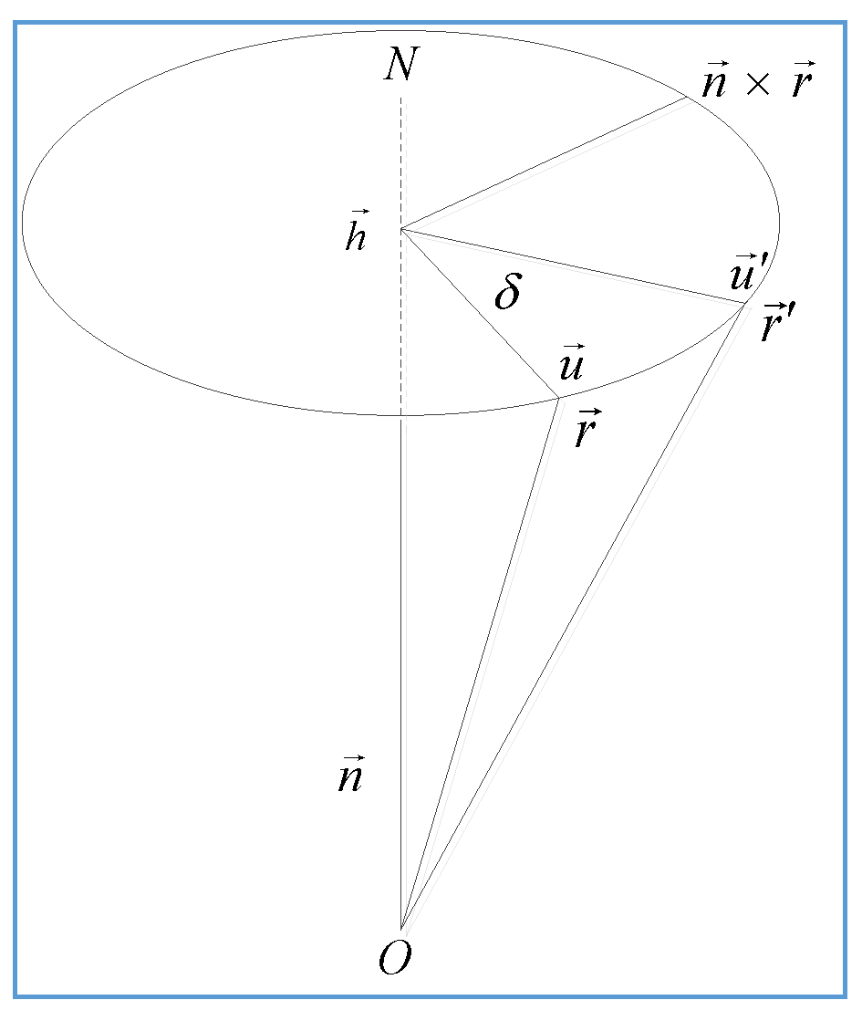
As is known, spatial transformation mainly consists of a rotation and a translation. However, unit quaternion can only represent the spatial rotation in three-dimensional space, as shown in Figure 1. Later, dual quaternion was presented to represent spatial rotation and translation simultaneously, as shown in Figure 2, in which two quaternions are integrated with the aid of a dual number. The first successful application of dual quaternion in estimating the unknown spatial transformation parameters was introduced by Walker et al. [15]. Based on the analysis of correspondences between dual quaternion-based and matrix-based representations, a single cost function was formulated, which enabled the simultaneous calculation of six parameters in point feature-based registration. Instead of estimating only the six transformation parameters, Wang et al. added the scale parameter to a single cost function, which enabled the simultaneous derivation of rotation, translation, and scale parameters [16]. Prošková et al. also introduced dual quaternion to represent spatial transformation; the presented approach was successfully applied for deriving the seven parameter-based transformation between two sets of three-dimensional coordinates [21,22].

Based on the above analysis, conclusions can be drawn that unit quaternion can only represent rotation in three-dimensional space; when it is applied in spatial transformation, such as the seven parameter-based Helmert transform, the rotation parameters must be estimated first, on which basis the translation parameters and the scale factor will later be estimated. In the case of errors being introduced into the estimation of the rotation parameters, the accuracy of the translation parameters and the scale factor will certainly be affected, which makes it a tendency that dual quaternions are introduced to represent spatial transformation.

2.2. Planar Feature-Based Registration Methods

Compared to point and linear features, planar features exist widely in those point clouds acquired from man-made buildings. On the condition that no specific man-made reflectors are used, point and linear features are often extracted by fitting and the intersection of adjacent planar features. Therefore, if planar features can be used directly in point cloud registration, the amount of calculation will be reduced greatly. In other words, the employment of planar features in point cloud registration will provide more conditions for estimating the transformation parameters than using point and linear features only. Of all existing planar feature-based registration methods, some use the distance between the point and its corresponding planar feature to construct error norms [6,23], others use the parallelism between the two normal vectors and the distance between the two conjugate planar features to construct error norms [7,24,25,26,27,28]. Detailed explanations are as follows: Grant et al. presented an iterative solution to pairwise point cloud registration, which is based on the correspondences between point and planar features [23]. Pavan et al. presented a closed-form solution to planar feature-based registration of terrestrial LiDAR point clouds [27], which was later applied in the global refinement for the terrestrial laser scanner (TLS) data registration [7]. Moreover, Wang et al. [24], Zhang et al. [25], and Previtali et al. [26] separately presented a planar feature-based registration algorithm based on the correspondences between each pair of planar features in which the Rodriguez matrix, Euler angles, and quaternions were, respectively, employed to represent spatial rotation. In addition, Khoshelham presented a closed-form solution to planar feature-based pairwise point cloud registration [6] in which the Kronecker product was employed to linearize the nonlinear equations; rigid transformation and similarity transformation are both given in detail; the parallelism between normal vectors of the two conjugate planar features was not fully utilized. Föstner and Khoshelham presented an optimal solution and three direct solutions for efficient motion estimation from plane-to-plane correspondences and provided an analysis of the accuracy of the solutions, comparing their performance with the classical iterative closest point (ICP) algorithm [28].

In general, few of the available methods incorporate the scale parameter in planar feature-based registration, which makes it difficult to apply them in the fusion of data from different sources. Moreover, some methods use point and planar features as registration primitives; the role of normal directions is neglected in the estimation of transformation parameters.

To summarize: (1) When unit quaternion is introduced to represent spatial rotation in point cloud registration, the accuracy of the translation parameters and the scale factor will surely be affected in the case of the introduction of errors in the estimation of rotation parameters; (2) Planar feature is a good alternative in point cloud registration, however, the determination of the difference between each corresponding planar feature is difficult with traditional mathematical expressions; (3) Few methods incorporate the scale parameters in the planar feature-based registration, which makes it difficult to apply them in the fusion of data from different sources; (4) Most available methods estimate the registration parameters by iterative calculation, the initial approximate estimates of the unknown parameters must be determined in advance to assist the linearization. Based on the above analysis, our goal was to develop a closed-form solution to a planar feature-based registration algorithm in which a quad tuple-based representation of planar features in three-dimensional space is given, which made it possible to directly determine the difference between each pair of corresponding planar features; dual quaternions were employed to represent the spatial transformation in three-dimensional space which made it possible to estimate all the registration parameters simultaneously. The scale factor was also considered in our registration methods, which made it possible to apply our method in the fusion of data from different sources.

3. Dual Quaternion-Based Transformation of Planar Features

3.1. Representation of a Plane in Three-Dimensional Space

Traditionally, a plane is represented by the normal vector $\overrightarrow{n}$ and any one point $\overrightarrow{p}$ lying on it. Since the selection of the point $\overrightarrow{p}$ is random, there is more than one representation for a single plane, which makes it difficult to compare and determine the difference between two planes. To ensure the unique representation of a plane in three-dimensional space, a quad tuple-based representation method was employed, as shown in Figure 3, in which a plane can be represented as a quad tuple $\widehat{\Gamma }$, as shown in Equation (1):

$$\widehat{\Gamma }=\left(\overrightarrow{l},m\right)$$

(1)

where $\overrightarrow{l}$ represents the normalized normal vector that forms $\overrightarrow{l}=\overrightarrow{n}/\Vert \overrightarrow{n}\Vert$, and $m$ represents the plane moment, that is, the distance between the origin and the plane that forms $m=\overrightarrow{p}\cdot \overrightarrow{l}$.

3.2. Definition of a Dual Quaternion

A quaternion is a composite of four real numbers, which is generally represented in the form of a quad tuple $\dot{r}$, as shown in Equation (2):

$$\dot{r}={\left(\begin{array}{cccc}{r}_0& r_1& r_2& r_3\end{array}\right)}^{\mathrm{T}}$$

(2)

on the condition that ${\dot{r}}^{\mathrm{T}}\dot{r}=1$, $\dot{r}$ is usually called a unit quaternion.

A dual quaternion is a composite of two quaternions and a dual number $\epsilon$, as shown in Equation (3):

$$\widehat{q}=\dot{r}+\epsilon \dot{s}$$

(3)

where $\dot{r}$ and $\dot{s}$ are both quaternions, each of which corresponds to the real part and the dual part of $\widehat{q}$ separately; when ${\dot{r}}^{\mathrm{T}}\dot{r}=1$, $\widehat{q}$ is a unit dual quaternion, which is the default definition of a dual quaternion.

3.3. Operation Rules for Dual Quaternions

Given two dual quaternions ${\widehat{q}}_1={\dot{r}}_1+\epsilon {\dot{s}}_1$ and ${\widehat{q}}_2={\dot{r}}_2+\epsilon {\dot{s}}_2$, the addition, subtraction, and multiplication between them can be expressed as shown in Equation (4):

$$\{\begin{array}{l}{\widehat{q}}_1+{\widehat{q}}_2=\left({\dot{r}}_1+{\dot{r}}_2\right)+\epsilon \left({\dot{s}}_1+{\dot{s}}_2\right)\\ {\widehat{q}}_1-{\widehat{q}}_2=\left({\dot{r}}_1-{\dot{r}}_2\right)+\epsilon \left({\dot{s}}_1-{\dot{s}}_2\right)\\ {\widehat{q}}_1{\widehat{q}}_2=\left({\dot{r}}_1+\epsilon {\dot{s}}_1\right)\left({\dot{r}}_2+\epsilon {\dot{s}}_2\right)={\dot{r}}_1{\dot{r}}_2+\epsilon \left({\dot{r}}_1{\dot{s}}_2+{\dot{r}}_2{\dot{s}}_1\right)\end{array}$$

(4)

Furthermore, multiplication between ${\dot{r}}_1$ and ${\dot{r}}_2$ can also be represented as shown in Equation (5):

$${\dot{r}}_1{\dot{r}}_2=\mathit{Q}\left({\dot{r}}_1\right){\dot{r}}_2=\mathit{W}\left({\dot{r}}_2\right){\dot{r}}_1$$

(5)

where $\mathit{Q}\left(\dot{r}\right)=\left[\begin{array}{cccc}{r}_0& -r_1& -r_2& -r_3\\ r_1& r_0& -r_3& r_2\\ r_2& r_3& r_0& -r_1\\ r_3& -r_2& r_1& r_0\end{array}\right]$, $\mathit{W}\left(\dot{r}\right)=\left[\begin{array}{cccc}{r}_0& -r_1& -r_2& -r_3\\ r_1& r_0& r_3& -r_2\\ r_2& -r_3& r_0& r_1\\ r_3& r_2& -r_1& r_0\end{array}\right]$.

3.4. Dual Quaternion-Based Transformation of Planar Features

According to the definition of a dual quaternion, the spatial transformation of a plane in three-dimensional space can be expressed as shown in Equation (6):

$${\widehat{\Gamma }}_a=\widehat{q}{\widehat{\Gamma }}_b{\widehat{q}}^{\ast }$$

(6)

where $\widehat{q}$ is the dual quaternion corresponding to the spatial transformation; ${\widehat{q}}^{\ast }$ is the conjugate of $\widehat{q}$ that forms ${\widehat{q}}^{\ast }={\dot{r}}^{\ast }+\epsilon {\dot{s}}^{\ast }$; ${\widehat{\Gamma }}_a$ and ${\widehat{\Gamma }}_b$ represent a pair of conjugate planar features, ${\widehat{\Gamma }}_a$ represents the one before transformation and ${\widehat{\Gamma }}_b$ represents the one after transformation.

To realize the dual quaternion-based similarity transformation, a plane should be represented as shown in Equation (7):

$$\widehat{\Gamma }=\dot{l}+\dot{m}$$

(7)

where $\dot{l}={\left(0,{\overrightarrow{l}}^{\mathrm{T}}\right)}^{\mathrm{T}}$, which corresponds the normal vector of the plane, and $\dot{m}={\left(m,{\overrightarrow{0}}^{\mathrm{T}}\right)}^{\mathrm{T}}$, which corresponds to the moment of the plane.

According to Chasles’ theorem [29], when the scale parameter is not considered, six independent parameters are needed to represent the transformation between two different coordinate frames. However, when a dual quaternion is used, there are eight parameters in total. Two constraints should be added to estimate the unknown parameters for the spatial similarity transformation, as shown in Equation (8):

$$\{\begin{array}{l}{\dot{r}}^{\mathrm{T}}\dot{r}=1\\ {\dot{r}}^{\mathrm{T}}\dot{s}=0\end{array}$$

(8)

where $\dot{r}$ is the quaternion that represents the spatial rotation and $\dot{s}$ is the quaternion that represents the spatial translation. The explanation in Equation (8) is that $\dot{r}$ is a unit quaternion and it is orthogonal to $\dot{s}$.

4. Planar Features-Based Registration Model

4.1. Construction of the Objective Functions

In three-dimensional space, the transformation of a plane can be expressed as shown in Equation (9):

$$\{\begin{array}{l}{\overrightarrow{l}}_a=\mathit{R}{\overrightarrow{l}}_b\\ m_a={\overrightarrow{p}}_a\cdot {\overrightarrow{l}}_a=\mu m_b+\overrightarrow{t}\cdot \mathit{R}{\overrightarrow{l}}_b\end{array}$$

(9)

where ${\overrightarrow{l}}_b$ and $m_b$ represent the normal vector and the moment of the plane before transformation, respectively; ${\overrightarrow{l}}_a$ and $m_a$ represent the normal vector and the moment after transformation, respectively; $\mathit{R}$, $\overrightarrow{t}$, and $\mu$ separately represent the transformation matrix, the translation vector, and the scale factor between the two coordinate systems.

With a dual quaternion, Equation (9) can be further expressed as Equation (10):

$$\{\begin{array}{l}{\dot{l}}_a=\dot{r}{\dot{l}}_b{\dot{r}}^{\ast }\\ {\dot{m}}_a=\mu {\dot{m}}_b+\frac{1}{2}\left(\dot{r}{\dot{l}}_b{\dot{r}}^{\ast }{\dot{t}}^{\ast }-\dot{t}\dot{r}{\dot{l}}_b{\dot{r}}^{\ast }\right)\end{array}$$

(10)

where $\dot{r}$ is the unit quaternion corresponding to the rotation matrix $\mathit{R}$, ${\dot{r}}^{\ast }$ is the conjugate of $\dot{r}$, ${\dot{l}}_a=\left(0,{\overrightarrow{l}}_a\right)$, ${\dot{l}}_b=\left(0,{\overrightarrow{l}}_b\right)$, ${\dot{m}}_a=\left(m_a,\overrightarrow{0}\right)$, and ${\dot{m}}_b=\left(m_b,\overrightarrow{0}\right)$.

Making $\dot{s}=\frac{1}{2}\dot{t}\dot{r}$, Equation (10) can be rewritten as Equation (11):

$$\{\begin{array}{l}{\dot{l}}_a=\dot{r}{\dot{l}}_b{\dot{r}}^{\ast }\\ {\dot{m}}_a=\mu {\dot{m}}_b-\dot{s}{\dot{l}}_b{\dot{r}}^{\ast }+\dot{r}{\dot{l}}_b{\dot{s}}^{\ast }\end{array}$$

(11)

where ${\dot{s}}^{\ast }$ is the conjugate of $\dot{s}$.

Based on Equation (7), Equation (11) can be further rewritten as Equation (12):

$$\{\begin{array}{l}{\dot{l}}_a=\mathit{W}{\left(\dot{r}\right)}^T\mathit{Q}\left(\dot{r}\right){\dot{l}}_b\\ {\dot{m}}_a=\mu {\dot{m}}_b-\mathit{W}{\left(\dot{r}\right)}^{\mathrm{T}}\mathit{Q}\left(\dot{s}\right){\dot{l}}_b+\mathit{W}{\left(\dot{s}\right)}^{\mathrm{T}}\mathit{Q}\left(\dot{r}\right){\dot{l}}_b\end{array}$$

(12)

Considering the existence of random errors, the planar feature-based registration approach aims to minimize the difference between $\left({\overrightarrow{l}}_a,m_a\right)$ and $\left({\overrightarrow{l}}_b,m_b\right)$. The quadratic form of the difference between $\left({\overrightarrow{l}}_a,m_a\right)$ and $\left({\overrightarrow{l}}_b,m_b\right)$ is introduced as the error equations according to the least squares criteria, as shown in Equations (13) and (14):

$$f_1{}^2={{\displaystyle \sum \left({\dot{l}}_a-\mathit{W}{\left(\dot{r}\right)}^{\mathrm{T}}\mathit{Q}\left(\dot{r}\right){\dot{l}}_b\right)}}^2$$

(13)

$$f_2{}^2={{\displaystyle \sum \left({\dot{m}}_a-\mu {\dot{m}}_b+\mathit{W}{\left(\dot{r}\right)}^{\mathrm{T}}\mathit{Q}\left(\dot{s}\right){\dot{l}}_b-\mathit{W}{\left(\dot{s}\right)}^{\mathrm{T}}\mathit{Q}\left(\dot{r}\right){\dot{l}}_b\right)}}^2$$

(14)

The transformation parameters can be obtained when the expression $f=f_1{}^2+f_2{}^2$ reaches its minimum. Considering that $f_1{}^2$ and $f_2{}^2$ are both positive, when each term reaches its minimum, $f$ will be minimal. The optimal value of $\dot{r}$ will be obtained by the minimization of Equation (13); $\dot{s}$ and μ will be obtained by the minimization of Equation (14).

4.2. Solution of Rotation Quaternions $\dot{r}$

Making $C_{l1}={\displaystyle \sum \left({\dot{l}}_a{}^{\mathrm{T}}{\dot{l}}_a+{\dot{l}}_b{}^{\mathrm{T}}{\dot{l}}_b\right)}$, ${\mathit{C}}_l=-2{\displaystyle \sum \mathit{Q}{\left({\dot{l}}_a\right)}^{\mathrm{T}}\mathit{W}\left({\dot{l}}_b\right)}$, Equation (13) can be decomposed as Equation (15):

$$f_1{}^2=C_{l1}+{\dot{r}}^{\mathrm{T}}{\mathit{C}}_l\dot{r}$$

(15)

Using Equation (5) as the restriction, the error function can be expressed as Equation (16):

$${\overline{F}}_1=C_{l1}+{\dot{r}}^{\mathrm{T}}{\mathit{C}}_l\dot{r}+{\lambda }_1\left({\dot{r}}^{\mathrm{T}}\dot{r}-1\right)$$

(16)

where ${\lambda }_1$ is a Lagrange multiplier constant.

Taking the partial derivative of Equation (16) yields Equation (17):

$$\frac{\partial {\overline{F}}_1}{\partial \dot{r}}=\left({\mathit{C}}_l+{\mathit{C}}_l^{\mathrm{T}}\right)\dot{r}+2{\lambda }_1\dot{r}=0$$

(17)

Making $\mathit{A}=-\frac{1}{2}\left({\mathit{C}}_l+{\mathit{C}}_l^{\mathrm{T}}\right)$, Equation (17) can be further expressed as Equation (18):

$$\mathit{A}\dot{r}={\lambda }_1\dot{r}$$

(18)

According to the definition of the eigenvalues and eigenvectors of a matrix, $\dot{r}$ represents one of the four eigenvectors of $\mathit{A}$, and ${\lambda }_1$ represents the corresponding eigenvalue of $\dot{r}$. Among the four eigenvectors that satisfy Equation (18), the optimal solution can be determined by referring back to Equation (17).

Multiplying Equation (17) with ${\dot{r}}^T$ yields Equation (19):

$${\dot{r}}^{\mathrm{T}}{\mathit{C}}_l\dot{r}=\frac{1}{2}{\dot{r}}^{\mathrm{T}}\left({\mathit{C}}_l+{\mathit{C}}_l^{\mathrm{T}}\right)\dot{r}=-{\lambda }_1$$

(19)

Substituting Equation (19) into Equation (16) yields Equation (20):

$${\overline{F}}_1=C_{l1}-{\lambda }_1$$

(20)

When ${\lambda }_1$ reaches its maximum, Equation (20) will be minimized. The conclusion can be drawn that the optimal solution of $\dot{r}$ equals to the eigenvector corresponding to maximum eigenvalue of $\mathit{A}$.

4.3. Solution of the Translation Quaternions $\dot{s}$ and the Scale Factor $\mu$

Making $C_1={\displaystyle \sum {\dot{m}}_a{}^{\mathrm{T}}{\dot{m}}_a}$, $C_2={\displaystyle \sum {\dot{m}}_b{}^{\mathrm{T}}{\dot{m}}_b}$, $C_3=-2{\displaystyle \sum {\dot{m}}_a{}^{\mathrm{T}}{\dot{m}}_b}$, ${\mathit{C}}_{m1}=2{\displaystyle \sum \mathit{I}}$, ${\mathit{C}}_{m2}=2{\displaystyle \sum \mathit{Q}{\left({\dot{m}}_a\right)}^{\mathrm{T}}\mathit{W}\left({\dot{l}}_b\right)}$, ${\mathit{C}}_{m3}=-2{\displaystyle \sum \mathit{W}{\left({\dot{l}}_b\right)}^{\mathrm{T}}\mathit{Q}\left({\dot{m}}_a\right)}$, $\underset{1\times 4}{{\mathit{C}}_{m4}}=-2{\displaystyle \sum {\dot{m}}_b{}^{\mathrm{T}}\mathit{W}{\left(\dot{r}\right)}^{\mathrm{T}}\mathit{W}\left({\dot{l}}_b\right)}$, $\underset{1\times 4}{{\mathit{C}}_{m5}}=2{\displaystyle \sum {\dot{m}}_b{}^{\mathrm{T}}\mathit{Q}\left(\dot{r}\right){\mathit{W}}^{\prime }\left({\dot{l}}_b\right)}$, ${\mathit{C}}_{m6}=-2{\displaystyle \sum \mathit{W}{\left({\dot{l}}_b\right)}^{\mathrm{T}}\mathit{W}\left(\dot{r}\right)\mathit{Q}\left(\dot{r}\right){\mathit{W}}^{\prime }\left({\dot{l}}_b\right)}$, and decomposing Equation (14), we can obtain Equation (21):

$$f_2{}^2=C_1+C_2{\mu }^2+{\dot{s}}^T\left({\mathit{C}}_{m1}+{\mathit{C}}_{m6}\right)\dot{s}+C_3\mu +{\dot{r}}^{\mathrm{T}}\left({\mathit{C}}_{m2}+{\mathit{C}}_{m3}\right)\dot{s}+\mu \left({\mathit{C}}_{m4}+{\mathit{C}}_{m5}\right)\dot{s}$$

(21)

Using Equation (5) as the restriction, the best quaternion $\dot{s}$ to represent the translation can be obtained when Equation (22) is minimized:

$${\overline{F}}_2=f_2{}^2+{\lambda }_2\left({\dot{r}}^{\mathrm{T}}\dot{s}\right)$$

(22)

where ${\lambda }_2$ is a Lagrange multiplier constant.

Taking the partial derivative of Equation (22), with respect to $\dot{s}$ and $\mu$, and making them equal to zero, we obtain Equations (23) and (24):

$$\frac{\partial {\overline{F}}_2}{\partial \dot{s}}=\left({\mathit{C}}_{m1}+{\mathit{C}}_{m1}^{\mathrm{T}}\right)\dot{s}+\left({\mathit{C}}_{m6}+{\mathit{C}}_{m6}^{\mathrm{T}}\right)\dot{s}+\left({\mathit{C}}_{m2}{}^{\mathrm{T}}+{\mathit{C}}_{m3}{}^{\mathrm{T}}\right)\dot{r}+\mu \left({\mathit{C}}_{m4}{}^{\mathrm{T}}+{\mathit{C}}_{m5}{}^{\mathrm{T}}\right)+{\lambda }_2\dot{r}=0$$

(23)

$$\frac{\partial {\overline{F}}_2}{\partial \mu }=2C_2\mu +C_3+\left({\mathit{C}}_{m4}+{\mathit{C}}_{m5}\right)\dot{s}=0$$

(24)

Based on Equation (24), the scale factor $\mu$ can be expressed as Equation (25):

$$\mu =-\frac{C_3+\left({\mathit{C}}_{m4}+{\mathit{C}}_{m5}\right)\dot{s}}{2C_2}$$

(25)

Substituting Equation (25) into Equation (23) yields Equation (26):

$$\dot{s}=-{\mathit{C}}_s{}^{-1}\left({\mathit{C}}_{m2}{}^{\mathrm{T}}+{\mathit{C}}_{m3}{}^{\mathrm{T}}\right)\dot{r}+\frac{C_3}{2C_2}{\mathit{C}}_s{}^{-1}\left({\mathit{C}}_{m4}{}^{\mathrm{T}}+{\mathit{C}}_{m5}{}^{\mathrm{T}}\right)-{\lambda }_2{\mathit{C}}_s{}^{-1}\dot{r}$$

(26)

where ${\mathit{C}}_s=\left({\mathit{C}}_{m1}+{\mathit{C}}_{m1}^{\mathrm{T}}\right)+\left({\mathit{C}}_{m6}+{\mathit{C}}_{m6}^{\mathrm{T}}\right)-\frac{\left({\mathit{C}}_{m4}{}^{\mathrm{T}}+{\mathit{C}}_{m5}{}^{\mathrm{T}}\right)\left({\mathit{C}}_{m4}+{\mathit{C}}_{m5}\right)}{2C_2}$.

Multiplying Equation (26) with ${\dot{r}}^{\mathrm{T}}$, we obtain Equation (27):

$${\dot{r}}^{\mathrm{T}}\dot{s}=-{\dot{r}}^{\mathrm{T}}{\mathit{C}}_s{}^{-1}\left({\mathit{C}}_{m2}{}^{\mathrm{T}}+{\mathit{C}}_{m3}{}^{\mathrm{T}}\right)\dot{r}+\frac{C_3}{2C_2}{\dot{r}}^{\mathrm{T}}{\mathit{C}}_s{}^{-1}\left({\mathit{C}}_{m4}{}^{\mathrm{T}}+{\mathit{C}}_{m5}{}^{\mathrm{T}}\right)-{\lambda }_2{\dot{r}}^T{\mathit{C}}_{\mathrm{s}}{}^{-1}\dot{r}=0$$

(27)

With Equation (27), ${\lambda }_2$ can be expressed as Equation (28):

$${\lambda }_2={\dot{r}}^{\mathrm{T}}\left({\mathit{C}}_{m2}{}^{\mathrm{T}}+{\mathit{C}}_{m3}{}^{\mathrm{T}}\right)\dot{r}+\frac{C_3}{2C_2}{\dot{r}}^{\mathrm{T}}\left({\mathit{C}}_{m4}{}^{\mathrm{T}}+{\mathit{C}}_{m5}{}^{\mathrm{T}}\right)$$

(28)

Since $\left({\mathit{C}}_{m2}{}^{\mathrm{T}}+{\mathit{C}}_{m3}{}^{\mathrm{T}}\right)$ is a skew-symmetric matrix, the first item of Equation (28) will be zero, that is, ${\dot{r}}^{\mathrm{T}}\left({\mathit{C}}_{m2}{}^{\mathrm{T}}+{\mathit{C}}_{m3}{}^{\mathrm{T}}\right)\dot{r}=0$. Equation (28) can be simplified, as shown in Equation (29):

$${\lambda }_2=\frac{C_3}{2C_2}{\dot{r}}^{\mathrm{T}}\left({\mathit{C}}_{m4}{}^{\mathrm{T}}+{\mathit{C}}_{m5}{}^{\mathrm{T}}\right)$$

(29)

The quaternion corresponding to the translation between the two neighboring LiDAR stations can be obtained using Equation (30):

$$\dot{t}=2\dot{s}{\dot{r}}^{\ast }$$

(30)

4.4. Implementation of the Proposed Solution

As in Figure 4, the given point clouds from the two neighboring LiDAR stations, namely the reference station and the unregistered station, suppose that $\left({\overrightarrow{l}}_a,m_a\right)$ and $\left({\overrightarrow{l}}_b,m_b\right)$ represent the two pairs of conjugate planar features separately extracted from them, where $\left({\dot{l}}_a,{\dot{m}}_a\right)$ and $\left({\dot{l}}_b,{\dot{m}}_b\right)$ are quaternion-based representations corresponding to $\left({\overrightarrow{l}}_a,m_a\right)$ and $\left({\overrightarrow{l}}_b,m_b\right)$. In the implementation of the proposed algorithm, the following steps are suggested to obtain the seven unknown parameters:

(1)

Based on the normal vectors of each pair of conjugate planar features, construct matrix A and calculate the maximum eigenvalue and its corresponding eigenvector $\dot{r}$ of A;

(2)

Calculate the quaternion $\dot{s}$ using Equation (26);

(3)

Calculate the scale factor $\mu$ using Equation (25);

(4)

Calculate the quaternion $\dot{t}$ using Equation (30).

Using $\dot{r}$, $\dot{s}$, and $\mu$, a plane in three-dimensional space can be transformed from one coordinate system to another. More importantly, since each pair of conjugate planar features is extracted from the two neighboring LiDAR stations, point clouds will be merged using $\dot{r}$, $\dot{s}$, and $\mu$.

5. Experiments and Results

The proposed planar feature-based registration algorithm was implemented using Matlab. Two experiments were designed to verify the correctness and the feasibility in which simulated data and real data were both incorporated.

5.1. Simulated Data

The first experiment was designed to verify the correctness of the proposed algorithm. Five pairs of simulated planar features were designed as shown in Figure 5. Mathematical descriptions of the simulated planar features were as shown in

Table 2. Mathematical descriptions of the simulated planar features.

Station	$\mathbf{Normal}\overrightarrow{\mathit{l}}$			$\mathbf{Passing}\mathbf{Point}\overrightarrow{\mathit{p}}$
	${\mathit{l}}_{\mathit{x}}$	${\mathit{l}}_{\mathit{y}}$	${\mathit{l}}_{\mathit{z}}$	${\mathit{p}}_{\mathit{x}}\left(\mathbf{m}\right)$	${\mathit{p}}_{\mathit{y}}\left(\mathbf{m}\right)$	${\mathit{p}}_{\mathit{z}}\left(\mathbf{m}\right)$
Reference Station	0.8503	0.4794	−0.2173	3.2755	3.7191	3.6741
	−0.4946	0.8689	−0.0184	1.5054	3.8689	3.9816
	0.1768	0.4856	0.2443	2.6377	3.3596	3.8370
	−0.3844	0.1692	0.3877	1.5549	3.7820	3.9834
	0.5032	−0.0879	0.2564	2.4251	3.2397	3.8914
Unregistered Station	1.0000	0.0000	0.0000	3.0000	0.0000	0.0000
	0.0000	1.0000	0.0000	0.0000	2.0000	0.0000
	0.3300	0.3300	0.3300	1.5000	0.0000	0.0000
	−0.3300	0.3300	0.3300	0.0000	1.8000	0.0000
	0.3300	−0.3300	0.3300	1.0000	0.0000	0.0000

. The pre-established spatial similarity transformation parameters were as shown in

Table 3. Pre-established spatial similarity transformation parameters.

Rotation Matrix R	$\mathbf{Translator}\overrightarrow{\mathit{T}}$			Scale Parameter μ
	${\mathit{T}}_{\mathit{x}}\left(\mathbf{m}\right)$	${\mathit{T}}_{\mathit{y}}\left(\mathbf{m}\right)$	${\mathit{T}}_{\mathit{z}}\left(\mathbf{m}\right)$
$\left[\begin{array}{ccc}0.8503& -0.4946& 0.1800\\ 0.4794& 0.8689& 0.1231\\ -0.2173& -0.0183& 0.9759\end{array}\right]$	2.000	3.000	4.000	0.5

.

The obtained transformation parameters were as shown in

Table 4. Registration results and residuals between each pair of conjugate planar features after registration.

Rotation Matrix R	$\mathbf{Translator}\overrightarrow{\mathit{T}}$			Scale Parameter μ	Residuals and RMSE
	${\mathit{T}}_{\mathit{x}}\left(\mathbf{m}\right)$	${\mathit{T}}_{\mathit{y}}\left(\mathbf{m}\right)$	${\mathit{T}}_{\mathit{z}}\left(\mathbf{m}\right)$		Normal				Moment
					Δlx	Δlx	Δlz	mΔl (×10−4)	Δm (m)	mΔm (×10−4)
$\left[\begin{array}{ccc}0.8503& -0.4946& 0.1800\\ 0.4794& 0.8689& 0.1231\\ -0.2173& -0.0184& 0.9759\end{array}\right]$	2.0001	3.0000	4.0001	0.5000	0.0191	0.0609	0.2090	3.0000	0.4399	6.2000
					−0.1243	−0.0714	−0.0289		−0.7919
					0.1743	−0.1594	0.1906		0.3048
					0.1149	0.3019	−0.0178		0.3810
					0.0886	0.2668	−0.0824		−0.6858

; the residuals between each pair of conjugate planar features after registration are also given.

Based on the results given in Table 4, the calculated rotation matrix and the scale factor were both consistent with the pre-established ones. The small deviation between the calculated translation vector and the pre-established one can be attributed to the rounding errors in the calculation, which can largely be ignored in practical applications. The conclusion can be drawn that the proposed solution is correct and the obtained result is as expected.

5.2. Real Data

The second experiment was designed to verify the feasibility of the proposed algorithm. The point clouds were collected by a model Riegl LMS-Z420i terrestrial laser scanner. In order to collect the complete point cloud data of the building, a total of eight observation stations were set up around it. The average distance between each observation station and the building was about 100 m, and the average sampling interval was set to 4 cm. Seven pairs of conjugate planar features were extracted from the two neighboring point clouds as shown in Figure 6, and the extracted planar features were as shown in

Table 5. Planar features extracted by least squares fitting.

Station	$\mathbf{Normal}\overrightarrow{\mathit{l}}$			$\mathbf{Passing}\mathbf{Point}\overrightarrow{\mathit{p}}$
	${\mathit{l}}_{\mathit{x}}$	${\mathit{l}}_{\mathit{y}}$	${\mathit{l}}_{\mathit{z}}$	${\mathit{p}}_{\mathit{x}}\left(\mathbf{m}\right)$	${\mathit{p}}_{\mathit{y}}\left(\mathbf{m}\right)$	${\mathit{p}}_{\mathit{z}}\left(\mathbf{m}\right)$
Reference Station	−0.706	0.7081	−0.0128	−70.7593	−6.3887	26.4681
	−0.7062	0.7079	−0.0108	−50.433	13.7874	22.2993
	−0.7103	−0.7039	−0.0006	−50.5877	14.9477	22.2911
	−0.006	0.009	0.9999	−61.8226	24.8605	25.7601
	−0.7044	0.7097	−0.0113	−63.6772	26.7793	16.8218
	−0.7072	−0.707	0.0013	−63.2206	27.6485	16.8952
	−0.0024	0.0142	0.9999	−61.5702	25.1852	22.593
Unregistered Station	−0.2579	0.9648	−0.0522	−63.6731	−7.892	15.175
	−0.2586	0.9647	−0.0503	−36.1147	−0.441	16.7593
	−0.9412	−0.2605	−0.2152	−35.7476	0.6642	17.2299
	−0.2194	−0.0081	0.9756	−41.3592	13.9261	19.8014
	−0.256	0.9654	−0.0508	−40.0006	17.5009	10.9515
	−0.9401	−0.2659	−0.2132	−39.2034	18.0633	11.1137
	−0.2123	−0.0054	0.9772	−40.4619	14.6743	16.7639

.

The obtained transformation parameters and residuals between each pair of conjugate planar features are both given in

Table 6. Registration results and residuals between each pair of conjugate planar features.

Scheme	Rotation Matrix R	$\mathbf{Translator}\overrightarrow{\mathit{T}}$			Scale Parameter μ	Residuals and RMSE
		${\mathit{T}}_{\mathit{x}}\left(\mathbf{m}\right)$	${\mathit{T}}_{\mathit{y}}\left(\mathbf{m}\right)$	${\mathit{T}}_{\mathit{z}}\left(\mathbf{m}\right)$		Normal				Moment
						Δlx	Δlx	Δlz	mΔl	Δm (m)	mΔm
Closed-form Solution	$\left[\begin{array}{ccc}0.8503& -0.4944& 0.1802\\ 0.4791& 0.8690& 0.1235\\ -0.2177& -0.0186& 0.9758\end{array}\right]$	−23.0132	29.3729	−2.2901	1.0000	−0.0003	−0.0003	0.0000	0.0008	0.0012	0.0307
						−0.0003	−0.0003	0.0000		−0.0071
						0.0000	0.0000	0.0003		−0.0391
						0.0007	0.0007	0.0000		−0.0352
						−0.0003	−0.0003	0.0005		0.0062
						−0.0008	0.0008	−0.0002		0.0394
						−0.0007	0.0000	0.0000		0.0352
Iterative Solution	$\left[\begin{array}{ccc}0.8504& -0.4943& 0.1802\\ 0.4790& 0.8691& 0.1234\\ -0.2176& -0.0186& 0.9759\end{array}\right]$	−23.0085	29.3766	−2.2902	1.0000	−0.0004	−0.0004	0.0000	0.0008	0.0012	0.0307
						−0.0004	−0.0004	0.0000		−0.0071
						0.0001	−0.0001	−0.0002		−0.0391
						0.0008	0.0008	0.0000		−0.0352
						−0.0004	−0.0004	0.0005		0.0062
						−0.0007	0.0007	−0.0001		0.0394
						−0.0006	0.0000	0.0000		0.0352

. To further verify the correctness and the feasibility of the proposed solution, a unit quaternion-based, iterative method [8] was employed to estimate the transformation parameters; the results are also shown in Table 6.

The visual effects of the point clouds from the two neighboring LiDAR stations before and after registration were as shown in Figure 5.

As shown in Table 6 and Figure 7, by using the obtained transformation parameters to register the two neighboring stations, there were no significant residuals between each pair of conjugate planar features after registration. More importantly, there were also no significant differences between the results obtained by our method and by the unit quaternion-based iterative method [8]; the root mean square error (RMSE) of the normal and moment’s differences between conjugate planar features were exactly the same. The conclusion can be drawn that the newly proposed closed-form solution to pairwise registration of LiDAR point clouds is correct and feasible.

6. Discussion

On the assumption that the normal directions of each pair of conjugate planar features are the same, the proposed quad tuple-based representation method can provide a unique mathematical expression of any planar feature in three-dimensional space; the differences between two planar features can be determined by direct comparison, which makes it convenient to propose and implement a closed-form solution to planar feature-based point cloud registration. The results of the two designed experiments were both correct, which proves that the proposed closed-form solution is capable of dealing with point cloud registration problems on the condition that sufficient corresponding planar features are provided as registration primitives.

It should be noted that any vector in three-dimensional space can be expressed in another form with the same module and an opposite direction; however, the prerequisite of our solution is that normal directions of each pair of conjugate planar features should be exactly the same after registration. On the condition that the prerequisite is not fulfilled, ensuring the proper run of the proposed solution will be one of our objectives in the future.

7. Conclusions

On the condition that point and linear features are not sufficient, planar features are good alternatives to ensure the proper run of the point cloud registration algorithm. Compared to point and linear features, extracting planar features from point clouds is more convenient. Furthermore, the impact of random errors can be significantly reduced by least squares fitting. Based on the quad tuple-based representation method of planar features in three-dimensional space, a closed-form solution to planar feature-based registration of point clouds is proposed. Two experiments were designed, in which both simulated data and real data were used to verify the correctness and effectiveness of the proposed solution. With the simulated data, the calculated registration results were consistent with the pre-established parameters and with the real data, there were also no significant differences between the results obtained by our method and by the available iterative method [8]; the root mean square error (RMSE) of the normal and moment’s differences between conjugate planar features were the same.

The conclusion can be drawn that the newly proposed closed-form solution to pairwise registration of LiDAR point clouds is correct and feasible. Moreover, the advantages of the proposed solution can be summarized as follows: (1) By using eigenvalue decomposition to replace the linearization of the objective function, the presented solution does not require any initial estimates of unknown transformation parameters in advance, which assures the stability and robustness of the algorithm; (2) On the condition that no man-made reflectors are used, planar features are directly extracted from point clouds using least squares fitting, the impact of random errors can be reduced significantly and the reliability of the estimated transformation parameters is higher than point and linear feature-based methods; (3) In contrast to Euler angle-based and rotation matrix-based methods, using dual quaternions to represent spatial rotation greatly reduces additional constraints in the estimation of similarity transformation parameters.

References

- Arun, K.S.; Huang, T.S.; Bostein, S.D. Least-squares fitting of two 3-D point sets. IEEE Trans. Pattern Anal. Mach. Intell. 1987, 9, 698–700. [Google Scholar] [CrossRef] [Green Version]
- Besl, P.J.; Mckay, N.D. A Method for Registration of 3-D Shapes. IEEE Trans. Pattern Anal. Mach. Intell. 1992, 14, 239–256. [Google Scholar] [CrossRef]
- Habib, A.; Ghanma, M.; Morgan, M.; Al-Ruzouq, R. Photogrammetric and LiDAR Data Registration Using Linear Features. Photogramm. Eng. Remote. Sens. 2005, 71, 699–707. [Google Scholar] [CrossRef]
- Wang, Y.; Yang, H.; Liu, Y.; Niu, X. Linear-Feature-Constrained Registration of LiDAR Point Cloud via Quaternion. Geomat. Inf. Sci. Wuhan Univ. 2013, 38, 1057–1062. [Google Scholar]
- Sheng, Q.; Chen, S.; Liu, J.; Wang, H. LiDAR Point Cloud Registration based on Plücker Line. Acta Geod. Cartogr. Sin. 2016, 45, 58–64. [Google Scholar]
- Khoshelham, K. Closed-form solutions for estimating a rigid motion from plane correspondences extracted from point clouds. ISPRS J. Photogramm. Remote. Sens. 2016, 114, 78–91. [Google Scholar] [CrossRef]
- Pavan, N.; Santos, D.; Khoshelham, K. Global Registration of Terrestrial Laser Scanner Point Clouds Using Plane-to-Plane Correspondences. Remote Sens. 2020, 12, 1127. [Google Scholar] [CrossRef] [Green Version]
- Wang, Y.B.; Zheng, N.S.; Bian, Z.F. A Quaternion-based, Planar Feature-constrained Algorithm for the Registration of LiDAR Point Clouds. Acta Opt. Sin. 2020, 40, 2310001. [Google Scholar] [CrossRef]
- Zheng, D.; Yue, D.; Yue, J. Geometric feature constraint based algorithm for building scanning point cloud registration. Acta Geod. Cartogr. Sin. 2008, 37, 464–468. [Google Scholar]
- Wang, Y.; Wang, Y.; Han, X. A Unit Quaternion based, Point-Linear Feature Constrained Registration Approach for Terrestrial LiDAR Point Clouds. J. China Univ. Min. Technol. 2018, 47, 671–677. [Google Scholar]
- Chai, S.; Yang, X. Line primitive point cloud registration method based on dual quaternion. Acta Opt. Sin. 2019, 39, 1228006. [Google Scholar] [CrossRef]
- Shen, Y.Z.; Chen, Y.; Zheng, D.H. A quaternions-based geodetic datum transformation algorithm. J. Geod. 2006, 80, 233–239. [Google Scholar] [CrossRef]
- Horn, B.K. Closed-form solution of absolute orientation using unit quaternions. J. Opt. Soc. Am. 1987, 4, 629–642. [Google Scholar] [CrossRef]
- Horn, B.K. Closed form solution of absolute orientation using orthonormal matrices. J. Opt. Soc. Am. 1988, 5, 1127–1135. [Google Scholar] [CrossRef] [Green Version]
- Walker, M.W.; Shao, L.; Volz, R.A. Estimating 3-D Location Parameters Using Dual Number Quaternions. CVGIP Image Underst. 1991, 54, 358–367. [Google Scholar] [CrossRef] [Green Version]
- Wang, Y.; Wang, Y.; Wu, K.; Yang, H.; Zhang, H. A dual quaternion-based, closed-form pairwise registration algorithm for point clouds. ISPRS J. Photogramm. Remote Sens. 2014, 94, 63–69. [Google Scholar] [CrossRef]
- Hamilton, W.R. On quaternions, or on a new system of imaginaries in algebra. Philos. Mag. 1844, 25, 489–495. [Google Scholar]
- Zeng, H.; Yi, Q. Quaternion-Based Iterative Solution of Three-Dimensional Coordinate Transformation Problem. J. Comput. 2011, 6, 1361–1368. [Google Scholar] [CrossRef]
- Joseph, J.; Laviola, J. A comparison of unscented and extended Kalman filtering for estimating quaternions motion. In Proceedings of the 2003 American Control Conference, Denver, CO, USA, 4–6 June 2003; pp. 2435–2440. [Google Scholar]
- Kim, A.; Golnaraghi, M.F. A quaternions-based orientation estimation algorithm using an inertial measurement unit. In Proceedings of the Position Location and Navigation Symposium, Monterey, CA, USA, 26–29 April 2004; pp. 268–272. [Google Scholar]
- Prošková, J. Application of dual quaternions algorithm for geodetic datum transformation. J. Appl. Math. 2011, 4, 225–236. [Google Scholar]
- Prošková, J. Discovery of Dual Quaternions for Geodesy. J. Geom. Graph. 2012, 16, 195–209. [Google Scholar]
- Grant, D.; Bethel, J.; Crawford, M. Point-to-plane registration of terrestrial laser scans. ISPRS J. Photogramm. Remote Sens. 2012, 72, 16–26. [Google Scholar] [CrossRef]
- Wang, L.; Li, G.; Zhang, Q. Plane Fitting and Transformation in Laser Scanning. J. Geomat. Sci. Technol. 2012, 29, 101–104. [Google Scholar]
- Zhang, D.; Huang, T.; Li, G.; Jiang, M. Robust Algorithm for Registration of Building Point Clouds Using Planar Patches. J. Surv. Eng. 2012, 138, 31–37. [Google Scholar] [CrossRef]
- Previtali, M.; Barazzetti, L.; Brumana, R.; Scaioni, M. Laser Scan Registration Using Planar Features. Int. Arch. Photogramm. Remote Sens. Spat. Inf. Sci. ISPRS Arch. 2014, 40, 501–508. [Google Scholar] [CrossRef] [Green Version]
- Pavan, N.L.; dos Santos, D.R. A global closed-form refinement for consistent TLS data registration. IEEE Geos. Remote Sens. Lett. 2017, 14, 1131–1135. [Google Scholar] [CrossRef]
- Föstner, W.; Khoshelham, K. Efficient and accurate registration of point clouds with plane to plane correspondences. In Proceedings of the IEEE International Conference on Computer Vision Workshops, Venice, Italy, 22–29 October 2017; IEEE Computer Society: Washington, DC, USA, 2017; pp. 2165–2173. [Google Scholar]
- Chasles, M. Note sur les Proprietes Generales du Systeme de Deux Corps Semblables entr’eux, Bullettin de Sciences Mathematiques. Astron. Phys. Chim. 1830, 14, 321–326. [Google Scholar]