Improving Geographically Weighted Regression Considering Directional Nonstationary for Ground-Level PM_2.5 Estimation

Abstract

The increase in atmospheric pollution dominated by particles with an aerodynamic diameter smaller than 2.5 μm (PM_2.5) has become one of the most serious environmental hazards worldwide. The geographically weighted regression (GWR) model is a vital method to estimate the spatial distribution of the ground-level PM_2.5 concentration. Wind information reflects the directional dependence of the spatial distribution, which can be abstracted as a combination of spatial and directional non-stationarity components. In this paper, a GWR model considering directional non-stationarity (GDWR) is proposed. To assess the efficacy of our method, monthly PM_2.5 concentration estimation was carried out as a case study from March 2015 to February 2016 in the Yangtze River Delta region. The results indicate that the GDWR model attained the best fitting effect (0.79) and the smallest error fluctuation, the ordinary least squares (OLS) (0.589) fitting effect was the worst, and the GWR (0.72) and directionally weighted regression (DWR) (0.74) fitting effects were moderate. A non-stationarity hypothesis test was performed to confirm directional non-stationarity. The distribution of the PM_2.5 concentration in the Yangtze River Delta is also discussed here.

1. Introduction

PM_2.5, which refers to particles with an aerodynamic diameter smaller than 2.5 μm, is one of the main indicators in air quality assessment [1]. Due to its small particle diameter, high capacity to carry viruses, long stagnation time in the atmosphere, and large transportation distance, PM_2.5 can not only cause a severe atmospheric environment with heavy haze but can also cause great harm to human lungs and respiratory and cardiovascular systems [2,3,4]. Accurate PM_2.5 spatial characterization is crucial to air quality assessment and addressing public health concerns, and a temporally continuous process at the monthly level is crucial to effectively conduct periodic air quality prediction and pre-disposal recommendations at medium and large scales. A large number of ground air quality monitoring stations have been established globally, and the monitoring of the spatial and temporal characteristics of PM_2.5 has become a hot spot. An unbalanced spatial distribution and incomplete coverage are the major obstacles to analysis and forecasting based on only discrete monitoring site data [5,6]. Satellite remote sensing can be used to assess the air quality in areas where ground-based PM_2.5 monitors are not available [7]. Since the middle of the 2000s, the MODIS (Moderate Resolution Imaging Spectroradiometer) and MISR (Multiangle Imaging Spectroradiometer) instruments onboard NASA’s Terra satellite have provided global observations of aerosol optical depth (AOD). Aerosol particles can block and attenuate the solar radiation reaching the ground by absorption, scattering, etc. AOD is the integral of the extinction coefficient of the medium in the vertical direction and describes the attenuation of light by aerosols [8]. According to the physical definition [9], AOD is related to the particles in the atmosphere. It has been demonstrated that AOD in the visible and near-infrared bands of inversion is most sensitive to particle concentrations of 0.1–2 μm in diameter, which is very close to the particle size range of PM_2.5 [10,11], thus providing an important theoretical basis for establishing the AOD–PM_2.5 correlation. Therefore, satellite remote sensing images are used to retrieve AOD data within a continuous spatial range and at a high spatial resolution, and a high-precision AOD–PM_2.5 spatial model has been discussed for ground PM_2.5 concentration estimation.

The classical AOD–PM_2.5 models include mechanistic and non-mechanistic models. Mechanistic models involve complex physicochemical processes and require the establishment of relatively complete models of emission sources, meteorological and pollutant dispersion processes, and other related physicochemical processes [12,13,14,15]. Non-mechanistic models, which capture data characteristics through historical data by statistical models or neural network models, are relatively simple and can easily be applied in practice [16,17,18,19,20,21]. The correlation between AOD and PM_2.5 has significant spatial non-stationarity [22]. Spatial non-stationarity means that the relationship between coefficients varies throughout space and cannot be explained by a simple global model [23]. Among the above models, the geographically weighted regression (GWR) model is a non-mechanistic technique that focuses on the non-stationarity spatial variability in linear regression modeling, making it prediction using the complex spatial structure of both predictor variables and their coefficients possible, and thus it can better reflect the complex spatial relationship between AOD and PM_2.5 over a certain contiguous region [23,24,25]. Numerous studies on PM_2.5 estimation have been conducted based on the GWR model. PM_2.5 prediction accuracy has been significantly improved in North America by introducing meteorological and land use variables [26]. To improve the regional scale of the PM_2.5 concentration estimation accuracy, Song [27] combined the AOD with vertically corrected relative humidity (RH) data to improve the AOD–PM_2.5 correlation. He and Huang [19] bridged the gap in 3-km AOD data via the development of the AOD image fusion technique and obtained daily PM_2.5 data in China at a 3-km resolution through estimation with the GTWR model, [28] indicating that the PM_2.5 concentration exhibits seasonal variation in China, while the winter pollution level is much higher than that in summer and other seasons.

The change in PM_2.5 concentration originates from pollution sources and air transportation. Wind is the main factor influencing PM_2.5 diffusion. Higher wind speeds impose a greater influence on the transport of air pollution, which is referred to as the wind effect [29]. Downwind areas of factories, for example, are more vulnerable to pollution emissions than are upwind areas. The wind effect influences the spatial heterogeneity of air pollution, in which the wind direction effect is manifested as the directional heterogeneity of spatial variation [30]. Jammalamadaka and Lund [31] confirmed wind heterogeneity through correlation analysis of the wind direction and PM_2.5. In most studies, the wind speed or direction has been adopted as an independent explanatory variable in simulation equations [32,33]. A relationship between PM_2.5 and the wind direction has been described largely with qualitative statistical charts, such as correlation analysis and qualitative discussion of the segmented wind direction and PM_2.5 using a wind frequency rose diagram [33,34]. A few studies have examined the influence of the wind field on the PM_2.5 concentration by equally considering the wind direction and wind speed to improve the interpolation accuracy [35,36,37].

Although these methods considering the wind influence have certain significance, the inaccurate definition of the wind classification, the lack of a quantitative wind–space relationship, and the incomplete utilization of wind information (especially the wind direction in vector format) may limit the further improvement of PM_2.5 estimation. In general, spatial and directional heterogeneity concepts have not been combined in regression models to estimate the PM_2.5 concentration. This paper first extends the traditional GWR model considering both spatial and directional non-stationarity.

2. Materials and Methods

2.1. Study Area

The Yangtze River Delta region is referred to as an economic zone including Shanghai, Jiangsu Province, and Zhejiang Province, as shown in Figure 1. The region is one of the most well-developed coastal areas in eastern China and one of the areas with the highest energy consumption, most intensive pollutant emissions, and most complex air pollution in China.

2.2. Materials

2.2.1. Ground-Level PM_2.5 Observations

Since 2010, China has gradually established air quality monitoring stations to provide real-time air quality monitoring data to the public. Data are available for more than 1600 air quality monitoring stations on the urban air quality real-time release platform established by the China Environmental Monitoring Station, which has officially been put into operation (http://106.37.208.233:20035/ (accessed on 20 December 2017)).

In this study, the obtained PM_2.5 data include the monthly average of 91 stations across the Yangtze River Delta from March 2015 to February 2016 (filtered from 108 stations with an average monitoring frequency greater than 25 times/month), for a total of 1040 records (filtered with an AOD greater than 0). The spatial distribution of the stations and their observed annual average PM_2.5 values are shown in Figure 1.

Since the measurement of PM_2.5 is conducted in a dry environment contrary to AOD, the PM_2.5 data were amended based on the RH to improve the linear relationship [27,38,39]. The correct equation is expressed as follows:

$$Corrected P{M}_{2.5}=P{M}_{2.5}\times \left(\frac{1}{1-RH/100}\right)$$

(1)

2.2.2. AOD Data

MODIS is a commonly considered instrument to retrieve AOD data, which is mounted on NASA Terra and Aqua satellites; it has a scan width of 2330 km and captures at least one global observation each day [40]. The instrument measures 36 spectral channels, with a spatial resolution range from 250 to 1000 m, and it is suitable to obtain aerosol, water vapor, surface temperature, and ocean data. The large number of spectral channels makes it possible to obtain parameters of aerosol particles of different sizes [41].

MODIS_L2 (level-2 atmospheric aerosol product) and MAIAC (Multi-Angle Implementation of Atmospheric Correction) are the main sources. According to comparative research, MAIAC products have a higher spatial resolution and coverage in China, but their values have significant bias. In eastern China, the MAIAC inversion has significant overestimation at low and medium values of aerosol optical thickness, due to errors in the calculation of regression coefficients for surface reflectance at different wavelengths [42]. In this study, we adopted the MOD04_L2 AOD data, which provide a full global coverage of aerosol properties resulting from the dark target (DT) and deep blue (DB) algorithms [43]. The DT algorithm was applied over ocean and dark land areas (e.g., vegetation), while the DB algorithm in Collection 6 (C6) covered all land areas, including both dark and bright surfaces. Both results are provided on a 10 by 10 pixels scale (10 km at the nadir). The component with the best assured quality (quality flag = 3) provided by MOD04_L2 was employed in this research area and was obtained from NASA Level-1 and the Atmosphere Archive and Distribution System (LAADS) website (http://ladsweb.nascom.nasa.gov/ (accessed on 20 December 2017)).

AOD data retrieved from MOD04_L2 should be extracted, clipped, reprojected, meshed, and spatially joined to obtain monthly average values and simultaneously remove any no-data values.

Subject to cloud influence, AOD data cover the space incompletely for each month, as shown in Figure 2, in which the change in pixel color from black to white indicates the increasing value of AOD, which was missing for some months. In this study, we effectively chose separate monthly AOD grids (filtered with an AOD greater than 0) for model fitting and spatially interpolated these by the kriging method for the final universal PM_2.5 estimation.

It has also been found that the original AOD can be vertically corrected by using the planetary boundary layer height (BLH) to achieve a better correlation with the ground-measured PM_2.5 concentration [11,38,39].

$$Corrected AOD=\frac{AOD}{BLH}$$

(2)

2.2.3. Wind Data

To estimate the whole region, regular continuous grids of wind field data must be generated. Wind information varies among grid units. Information can be acquired from available weather grid products or spatially interpolated from sample wind monitoring sites. Wind vector data contain v- and u-wind components in the Cartesian coordinate system, as shown in Figure 3. The wind direction in each grid can be calculated with Equation (3), starting from the north in the clockwise direction. The wind speed can be calculated with the square root of the sum of the u and v squares.

$$Win{d}_{dir}=0.5\pi -\arctan 2\left(vwind,uwind\right)$$

(3)

2.2.4. Auxiliary Data

In addition to the RH and BLH mentioned above, other factors related to PM_2.5 include the wind speed, wind direction, and temperature. Wind information at a height of 2 m, divided into u and v components, and the temperature were acquired from Copernicus Atmosphere Monitoring Service (CAMS) near-real-time data with a 0.125 degrees resolution (http://apps.ecmwf.int/datasets/data/cams-nrealtime/levtype=sfc/ (accessed on 20 December 2017)). BLH data were acquired from ERA Interim, namely, monthly averages of daily mean data, with a 0.75 degrees spatial resolution (http://apps.ecmwf.int/datasets/data/interim-full-moda/levtype=sfc/ (accessed on 20 December 2017)). The RH at 2 m was retrieved from NASA/POWER agroclimatology daily averaged data with a 1.0 degrees spatial resolution (http://power.larc.nasa.gov/common/AgroclimatologyMethodology/Agro1d0_Methodology_Content.html (accessed on 20 December 2017)).

2.2.5. Data Integration

All these data must be integrated into the same regular grids for regression calculation purposes. In this study, we defined the research scale at 10 × 10 km², covering 2570 square grids in the Yangtze River Delta region. In regard to the other data, the ordinary kriging interpolation method was applied to attain raster data with the same accuracy, and the point extraction method was adopted to extract the value in each grid, while the spatial connections between the independent variables and location information were considered during integration into the grids. Figure 4 shows our data processing workflow.

2.3. Methods

2.3.1. Geographically Weighted Regression Model (GWR)

The GWR model is a spatial statistical model suitable for spatial heterogeneity analysis [44]. The GWR model can be written as

$$Y_i={\beta }_0\left(u_i,v_i\right)+{\displaystyle \sum _k{\beta }_k\left(u_i,v_i\right)x_{ik}}+{\epsilon }_i$$

(4)

where $\left(u_i,v_i\right)$ are the coordinates of the $i$-th point, ${\beta }_0\left(u_i,v_i\right)$ represents the constant term, ${\beta }_k\left(u_i,v_i\right)$ is the $k$-th regression parameter at sampling point $i$, which is calculated via the weight function, and $x_{ik}$ represents the $k$-th coefficient value of the $i$-th point. ${\epsilon }_i$ is the error term for observation $i$, which is generally assumed to be normally distributed with a zero mean and constant variance.

In equation, it is assumed that the observations nearer to location $i$ are more influential on the estimates of ${\beta }_k\left(u_i,v_i\right)$.

$$\widehat{\beta }\left(u_i,v_i\right)={\left(X^{T}W\left(u_i,v_i\right)X\right)}^{-1}{X}^{T}W\left(u_i,v_i\right)Y$$

(5)

where $\widehat{\beta }$ is the estimated value of $\beta$, $W\left(u_i,v_i\right)$ comprises off-diagonal elements that are zero and diagonal elements that are the geographical weights of the n observed data points at regression point $i$, and $Y$ denotes the real dependent variable value.

The global linear regression model (OLS) is assigned a weight of 1. The initial step of the weighting-based local model excludes the observations beyond a certain distance $d$ from the regression point. The weighting function can be written as

$$w_{ij}=\exp {\left[-{\left(\frac{d_{ij}}{h}\right)}^2\right]}^2$$

(6)

where $j$ is a specific point in space at which data are observed, $i$ denotes any points in space for which parameters are estimated, $h$ is the bandwidth, and $d_{ij}$ is the distance in the Euclidean space. The bandwidth $h$ either remains fixed or is adapted to fit sample points under different spatial distribution conditions. For a given sample point, the fixed method yields an invariable spatial distance, while the adaptive method usually yields invariable nearest neighbor sample counts, resulting in bandwidth changes based on the sample density in space. Consequently, the fixed method is suitable for spatially balanced sample data, and the adaptive method is suitable for other sample data.

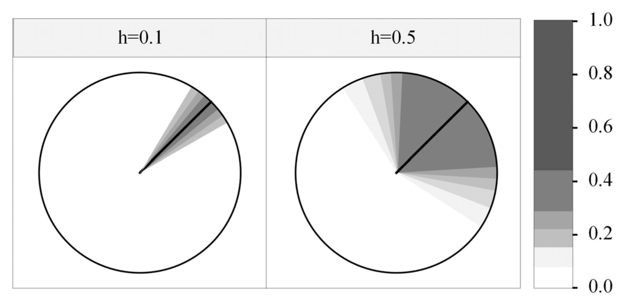
2.3.2. Directionally Weighted Regression Model (DWR)

In order to account for directional heterogeneity, R. Oller [35] presented a directional weighting function according to Equation (7) by defining the distance between two points’ directional difference.

$$d_{ij}=Angle\left(i,j\right)=\left|{\theta }_i-{\theta }_j\right|$$

(7)

The kernel model above can be applied to the locally weighted regression as well. Due to the effect of directional heterogeneity, points with a closer direction value should generate a stronger mutual influence. The bandwidth $h$ controls the impact between two samples in the direction unit of measurement, and spatial units close to the direction of the estimation point increase their weight (Figure 5).

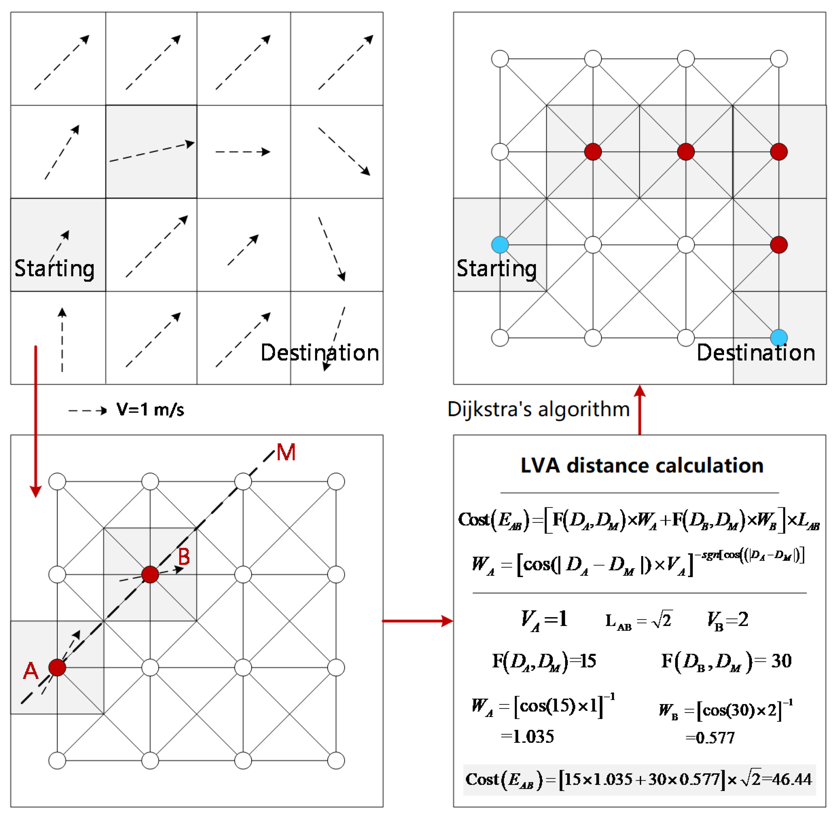
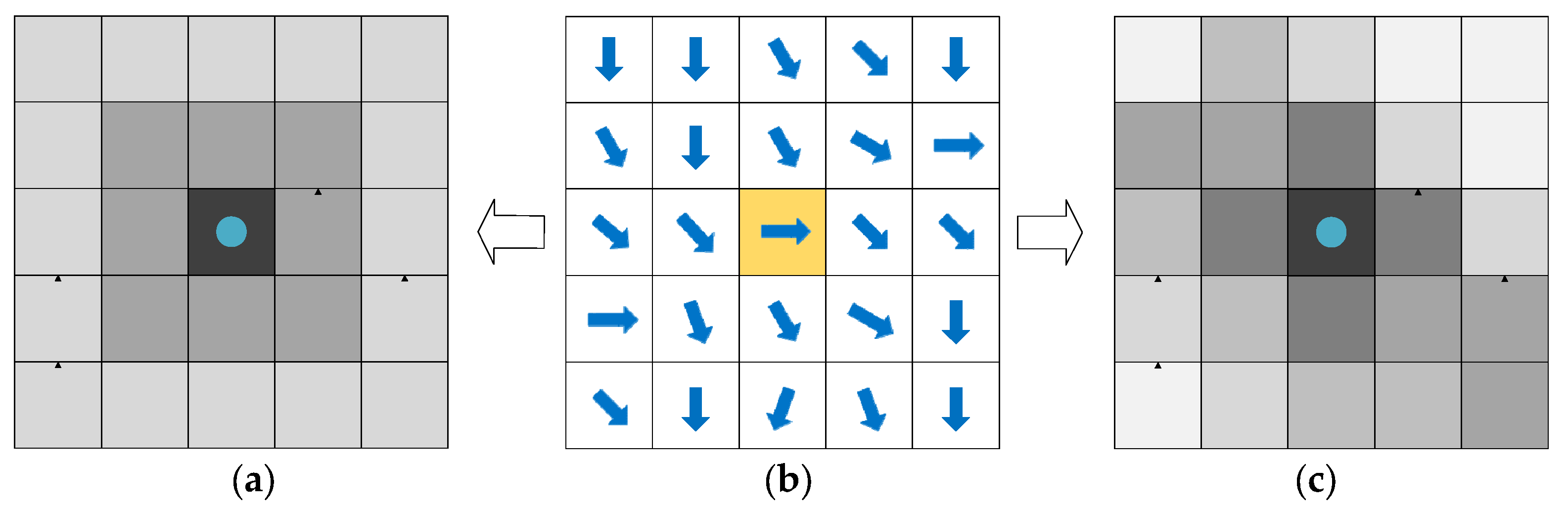
2.3.3. Extending the GWR Model Considering the Wind Influence (GDWR)

The wind direction imposes a major effect on PM_2.5 diffusion. Pollutants in air usually travel along the wind direction, which directly impacts the direction of pollutant diffusion. Therefore, the diffusion distance due to different wind directions varies, and the distance of pollution diffusion is also inconsistent. The wind speed also greatly influences the diffusion of pollutants. Generally, the higher the wind speed, the larger the diffusion distance and influence area of air pollutants. Therefore, the effect of the wind field on the PM_2.5 concentration is fundamentally reflected in the diffusion process of pollutants, which is characterized by wind direction and speed weighting.

In spatial regression, the influence of the wind field on the PM_2.5 concentration is embodied in the anisotropic characteristics of spatial variation and the directional aspect of spatial dependence. Based on the principle of non-stationarity, the directionality of spatial differentiation is determined. This method considers that the attenuation mode of the regression coefficient is subject to directional constraints, and the regression coefficients along the different directions are inconsistent with the corresponding distance attenuation.

The wind field affects the direction of atmospheric diffusion, and the spatial distance affects the diffusion intensity, such that the distance equation considering the space and direction can be integrated into the distance of atmospheric diffusion. This study adopted the direction of the atmospheric diffusion distance proposed by Li et al. [36,37] to consider both spatial and directional heterogeneity. The diffusion distance can be adopted to describe the difficulty of diffusion of air pollutants between adjacent grid units. Therefore, the distance is based on the standard model of air pollutant diffusion in the wind field–Gaussian diffusion model, as shown in Figure 6.

$\mathrm{Cos}t\left(E_{AB}\right)$ denotes the diffusion distance between two adjacent grids $A$ and $B$, the $\mathrm{F}$ function indicates the angle between the two wind directions, $D_A$ is the wind direction of grid $A$, and $D_M$ is the direction of line $AB$. $\cos \left(\left|D_A-D_M\right|\right)$ is the wind component rate along the $AB$ direction, and $V_A$ and $V_B$ are the wind speeds in grid units $A$ and $B$, respectively. The equation $-\mathrm{sgn}[\cos \left(\left|D_A-D_M\right|\right)$ determines the positive or negative effect on diffusion. For $\cos \left(\left|D_A-D_M\right|\right)>0$ the grid $A$ component of the wind speed along the $AB$ direction is positive, which exerts a positive impact on the diffusion process of pollutants, thus decreasing the diffusion distance. In contrast, for $\cos \left(\left|D_A-D_M\right|\right)\le 0$, the wind speed in grid $A$ results in a larger diffusion distance. $L_{AB}$ indicates the spatial distance between cells $A$ and $B$, which is calculated by the adjacency relation, $L_{AB}=1$ if the adjacency relation is edge-connected, or $L_{AB}=\sqrt{2}$ if the diagonal relation is point-connected.

In contrast to the effects of the upper and lower tuyeres proposed by Li et al. [37], this paper considered that the influences are equivalent with the same difficulty, and the smaller value was adopted as the final diffusion distance. In regard to grid data with arbitrary distances from points $i$ to $j$, the distance considering the wind field can be obtained with Dijkstra’s shortest path algorithm as follows:

$$d_{ij}=d_{wind}\left(p_i,p_j\right)=\underset{}{\min }{\displaystyle \sum }_i^j\min \left\{\mathrm{Cos}t\left(E_{AB}\right),\mathrm{Cos}t\left(E_{BA}\right)\right\}$$

(8)

Considering the combination of directional and spatial non-stationarity aspects, the wind field distance is defined accounting for the direction and spatial heterogeneity, namely, the wind field locally varying anisotropy (LVA) distance, in the PM_2.5 estimation model.

Selecting the Gaussian kernel function as an example, its weight calculation equation is

$$w_{ij}=\exp {\left[-{\left(\frac{d_{wind}\left(p_i,p_j\right)}{h}\right)}^2\right]}^2$$

(9)

where $h$ is the optimal bandwidth value expressed in units of the optimal wind field distance.

Figure 7 compares the expression form of the center point in the Euclidean distance space and the weight change in the wind field distance space. In the Euclidean distance space, it is expressed as a circular shape with the sample point as the center, and the distance in space increases with decreasing weight. In the wind field distance space, it is expressed as a band form with the sample point as its center, and the weight decreases along the shortest path of the wind field, which reflects its anisotropy.

According to the above defined formula and chart, it can be found that OLS, GWR, DWR, and GDWR models are specialized in solving general problems based on global linear assumptions, geographic problems based on spatial heterogeneity, problems based on directional heterogeneity, and geographic problems based on spatial plus directional heterogeneity, each with its own usage scenarios and specialties. In addition, these four models have sequential extension characteristics, and the extended model contains the capabilities of the original. That is, GWR and DWR are an extension of the OLS model separately, and GDWR is an extension of combined GWR and DWR models.

2.3.4. Parameter Estimation

Due to the uneven distribution of ground PM_2.5 monitoring sites, we adopted an adaptive Gaussian kernel in locally weighted regression for experimental verification. The distance in Equation (7) may be the Euclidean, directional, or diffusion distance. The optimal solution of the model depends on the definition of the bandwidth, and the current criteria considered for bandwidth selection include cross-validation (CV), Akaike information criterion (AIC) validation, and Bayesian information criterion (BIC) validation. The AIC has the advantage of a more general application than that of CV statistics [45]. In this study, we chose the AIC according to the following definition:

$$AI{C}_C=2n{\log }_e\left(\widehat{\sigma }\right)+n{\log }_e\left(2\pi \right)+n\left\{\frac{n+tr\left(S\right)}{n-2-tr\left(S\right)}\right\}$$

(10)

2.3.5. Result Evaluation

To test the effectiveness of the regression models, a homogeneity assumption assessment method must be developed, where F statistics are suitable to evaluate the model significance. Leung et al. [46] improved the existing traditional testing procedures of spatial non-stationarity in the GWR model. Here, we adopted this method to check the significant spatial and/or temporal non-stationarity over the study area before applying these models. The equation is given as follows, which is an F statistic using the method of analysis of variance:

$$F_2=\frac{\left(RS{S}_o-RS{S}_g\right)/v_1}{RS{S}_o/\left(n-p-1\right)}$$

(11)

where $F_2$ denotes the test statistic value, is $RS{S}_o$ the residual sum of squares of the ordinary least squares (OLS) model, RSS_g is the residual sum of squares of the locally weighted model, $v_1=tr\left(A\right)$, for $A=n-p-1-tr\left[{\left(I-L\right)}^{\mathrm{T}}\left(I-L\right)\right]$, $p$ is the count of explanatory variables, and $L$ is the hat matrix of the model.

Two indexes were used to evaluate the accuracy of the model fitting results and compare them with among different models: the root mean square error (RMSE) and the adjusted $R^2$($R_{adj}^2$). Equation (12) represents the expression of RMSE, where $y_i$ is the true monitored value and $\widehat{y_i}$ is the mode fitted value.

$$RMSE=\sqrt{\frac{1}{n}{\displaystyle \sum }_{i=1}^n{\left(y_i-\widehat{y_i}\right)}^2}$$

(12)

Equation (13) represents the expression of $R_{adj}^2$. The use of $R_{adj}^2$ is a modification of $R^2$ to avoid the index automatically and spuriously increasing when extra explanatory variables are included.

$$R_{adj}^2=1-\frac{VA{R}_E}{VA{R}_T}=1-\left(1-R^2\right)\frac{n-1}{n-p-1}$$

(13)

3. Results and Discussion

3.1. Model Definition

The OLS and GWR model structures can be expressed as

$$Corrected P{M}_{2.5}~corrected AOD+TEMP+RH+BLH+WIND$$

(14)

The DWR and GDWR model structures can be expressed as

$$Corrected P{M}_{2.5}~corrected AOD+TEMP+RH+BLH$$

(15)

Among them, the DWR, GWR, and GDWR models all adopt the Gaussian model as their kernel and apply the AIC equation as their optimal bandwidth selection criterion.

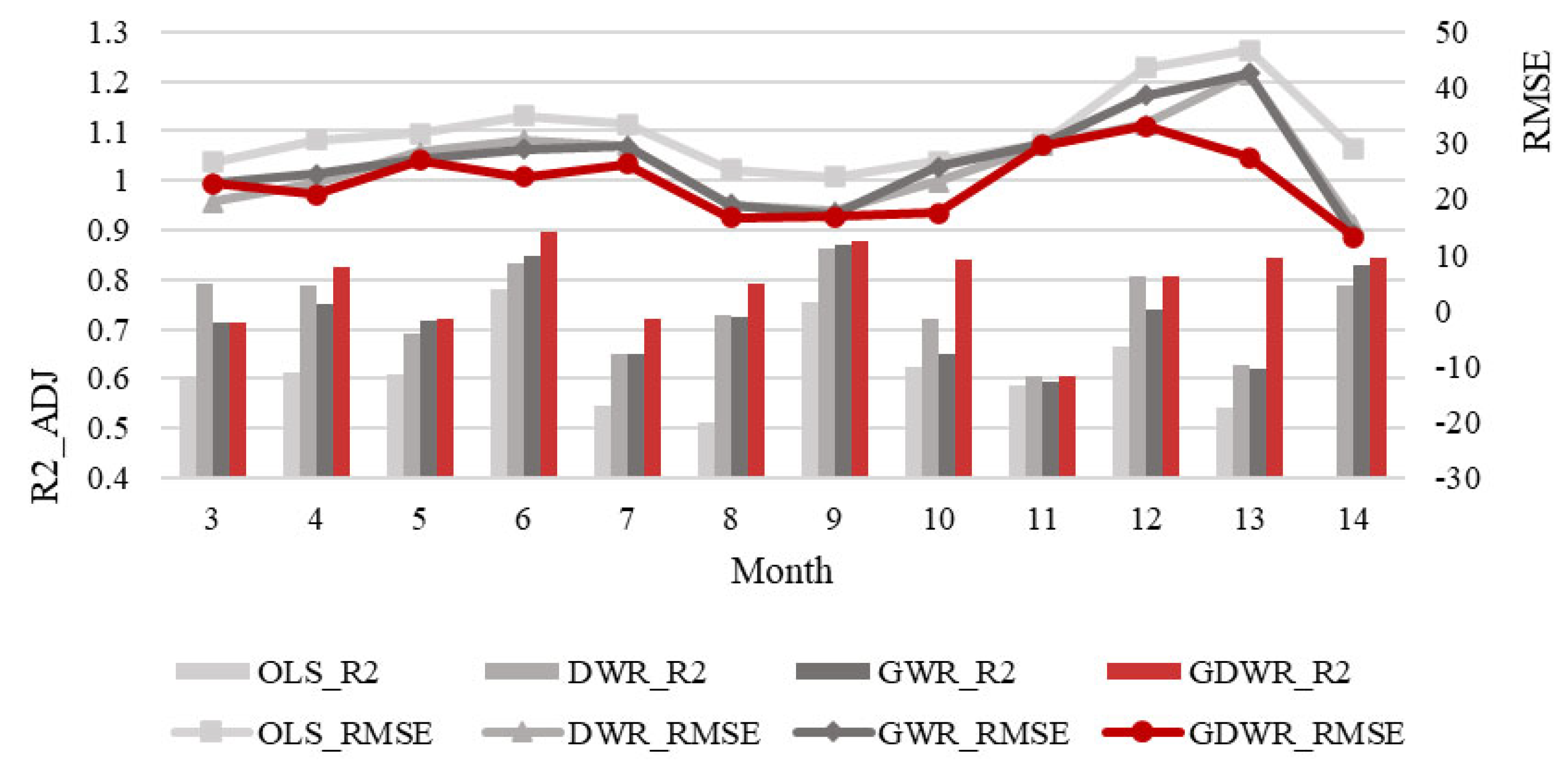
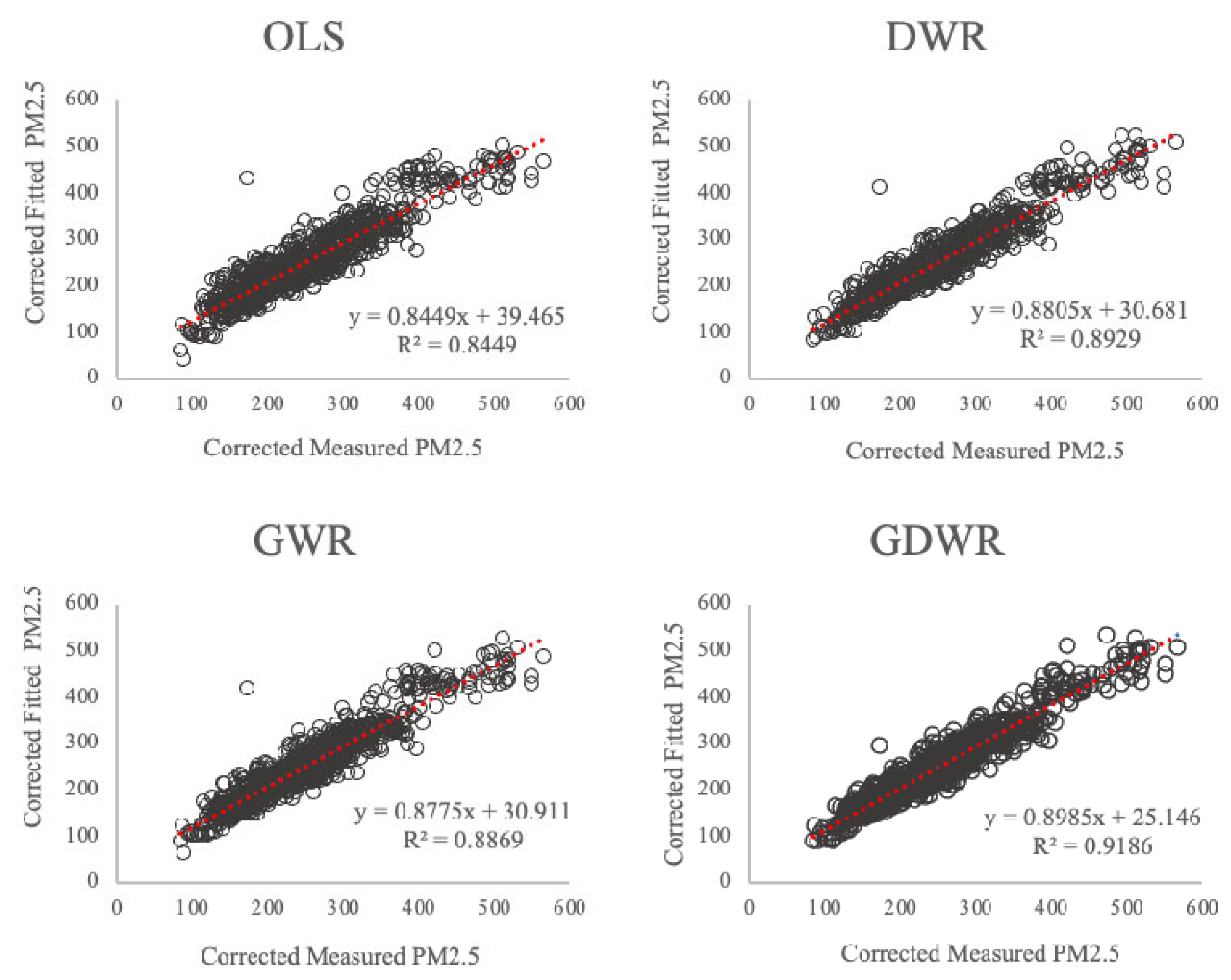
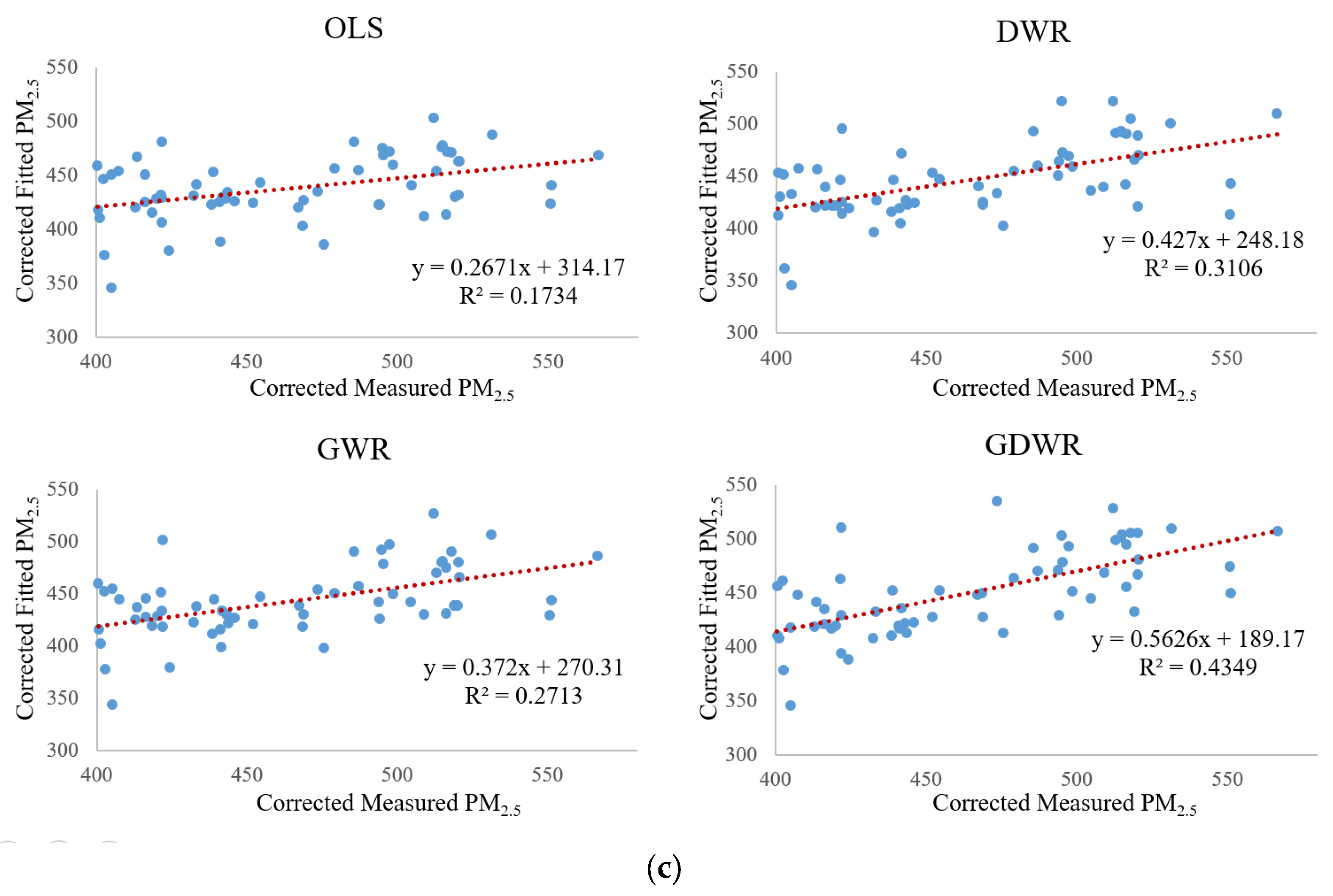
3.2. Accuracy of the Models

The model accuracy of the four types of models is shown in Figure 8. The revised PM_2.5 and AOD data generated a high fitting precision, except the OLS method. For example, in February 2016, the fitting precision of the OLS model only reached 0.2. Generally, the remaining models attained a precision above 0.5, with more than half of the fitting precision values higher than 0.8, indicating a good fitting effect. The RMSE exhibited a strong negative correlation with the fitting accuracy. Generally, the RMSE indicated a high fitting accuracy from March 2015 to November 2015, while the fitting effect declined during the autumn/winter transition period of 2015.

By comparing the four models, both the RMSE and $R_{adj}^2$ followed the order of GDWR>GWR≈DWR>OLS in terms of the model accuracy. The mean fitting accuracy values of the GDWR, GWR, DWR, and OLS models were 0.79, 0.72, 0.74, and 0.589, respectively.

From the perspective of the DWR model, its accuracy obviously exceeded that of the OLS model and was similar to that of GWR, indicating that the importance of wind direction modeling in the PM_2.5 regression exceeded the effect of the wind speed variable. Moreover, this also confirmed the occurrence of directional non-stationarity in the process of PM_2.5 regression modeling. The data comprising sample points with the same wind direction exhibited more similar characteristics of the regression coefficient, and the model fitting efficiency of the regression model that considered the directional value was higher.

From the perspective of the GDWR model, the optimal fitting effect was achieved in each month during the study period. Compared to the GWR model, the annual average accuracy increased by 9.7%, and the RMSE was reduced by 13.7%. Compared to the OLS model, the accuracy was 22% higher and the RMSE was 28.2% lower. Compared to the DWR model, the precision was 6.8% higher, and the RMSE was 11.9% lower. The wind field distance was adopted to comprehensively consider the wind direction, wind speed, and spatial distance information, and spatial and directional non-stationarity aspects were effectively combined to improve the model accuracy and realize PM_2.5 estimation with a higher accuracy.

When analyzed from a seasonal perspective, the fitting accuracy of all models seems to be highly dependent on the season, with a larger error in winter. This may be due to several reasons: The severe weather conditions in winter and spring can lead to very drastic changes in the vertical profile of aerosols, resulting in a complex and variable relationship between AOD and PM_2.5. The dispersion of the data varies from season to season, and the data values of PM_2.5 have obvious jumps in the more polluted weather. Since the boundary layer is often in inverse temperature in winter, it is difficult for heating emission aerosol particles to diffuse, resulting in a significant increase in the number of severely polluted days, which makes the model built with the overall data inaccurate for predicting some extreme values.

When analyzed on a monthly scale, the GDWR model stands out in Month 13. By counting the wind speed data for each month in the study area, results show that the variance of the wind speed in Month 13 (3.09) was second only to April (1.56) and May (1.74), but the wind speeds in these two months were relatively low with monthly average wind speeds of 1.4 m/s and 2.3 m/s, while the average wind speed in Month 13 was higher at 3.48 m/s, and the variance in all other months was significantly higher than those three months. It can be speculated that the wind speed distribution is relatively uniform over 13 months, there is a certain number of sample sizes at different wind speeds, and the wind speed again significantly changes the proximity metric values between stations, showing a large accuracy improvement.

3.3. Hypothesis Testing

The validity of the various models is verified and the results are listed in

Table 1. Comparison of F₂ test results.

Month	DWR	GWR	GDWR
3	2.220	2.466	2.898
4	2.143	3.942	2.306
5	1.628	2.079	1.921
6	2.264	3.011	1.687
7	2.133	2.464	1.995
8	1.791	2.500	1.891
9	2.438	2.759	3.094
10	1.574	2.331	1.755
11	1.005	1.897	1.261
12	2.411	2.773	1.941
13	1.884	2.690	2.016
14	2.556	2.745	2.211

. All of the models exhibit a significant rejection of the hypothesis test, indicating model validity, while the order was DWR≈GDWR>GWR in general. In contrast, the validity of the DWR and GDWR models exceeds that of the GWR model, which verifies the occurrence of spatial and directional non-stationarity.

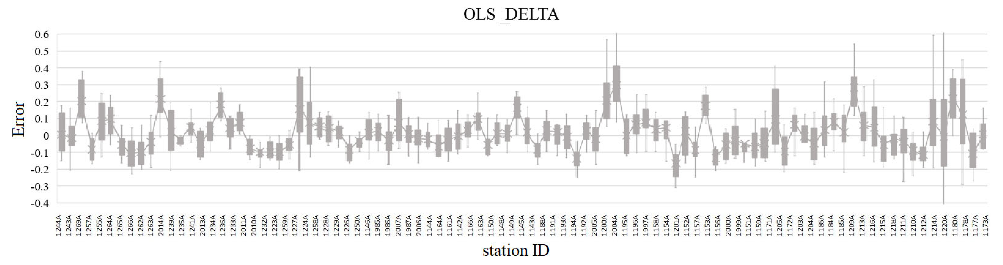
3.4. Accuracy at Each Site

To further evaluate the performance of the GDWR model, all the PM_2.5 measurements retrieved from monitoring stations were applied as a training dataset. The figure below shows the mean difference between the GDWR estimations and ground measurements, and the observed PM_2.5 discrepancies varied.

To analyze the model accuracy in greater detail, for each model, a two-dimensional scatter plot was generated for each PM_2.5 monitoring station according to the fitting results of the whole month and the actual monitoring values, and the model accuracy was graphically analyzed. The statistical results of each model are shown in Figure 9.

According to the above scatter plot of the model fitting results, PM_2.5 and the other independent variables all exhibited a notable fitting effect, and the PM_2.5 fitting accuracy between each model and the original calibrated data was above 0.8, indicating the validity of the models. Moreover, a comparison of the effects of these four models also revealed that the accuracy values followed the order of GDWR>DWR>GWR>OLS, indicating that the weighted regression model considering the annual direction achieved a higher fitting effect.

After recalculating the data into three segment groups by corrected PM_2.5 values (0~200, 200~400, 400~600), the statistical results of each model are shown in Figure 10. As seen in the figure, all models have the highest fitting accuracy in the PM_2.5 interval (200, 400), followed by the PM_2.5 interval (200, 400), and the worst in the high PM_2.5 interval (400,600), which is inversely proportional to the amount of effective training data in the interval. The number of effective training data for the high PM_2.5 value is significantly less than the other two intervals, resulting in a model accuracy below 0.5. Comparing between models, the GDWR model ranks first in all intervals, especially in the case of low training data, reflecting its strong resistance to missing training data.

Regarding the results of all models, the error at each site was obtained by generating a box diagram at the annual scale based on the error ratio between the real and predicted values at each site.

The error rate equation is

$$ErrorRate=\frac{Corrected Measured PM2.5-Corrected Fitted PM2.5}{Corrected Measured PM2.5}$$

(16)

The results are shown in Figure 11.

Analysis of the above box plot reveals that the error responses of the four types of models at all stations throughout the year are similar, with the number of stations on the abscisic coordinate generating similar error curves, which indicates that the model fitting degree at all PM_2.5 monitoring stations exhibits the same reaction in space. Statistics show that the fitting accuracy at most sites is consistently high over 12 months, which is reflected by the fact that the error value varies around the zero axis within a small range, and only a small proportion of the site data exhibit a wide error range. Moreover, the box height is large, and only a small fraction of the site errors is large. By comparing the error responses of the different models, the OLS model yields the largest mean error and the largest fluctuation range in the whole year, which indicates that the model accuracy is relatively low from a microscopic perspective. The DWR and GWR models basically attain the same performance. The GDWR model yields the smallest overall error at each site, and its fluctuation is smaller than that of the OLS, DWR, and GWR models. Based on the microscale response among the stations, it is found that, on the whole, the GDWR model achieves a better fitting effect than the other three models at all locations in space.

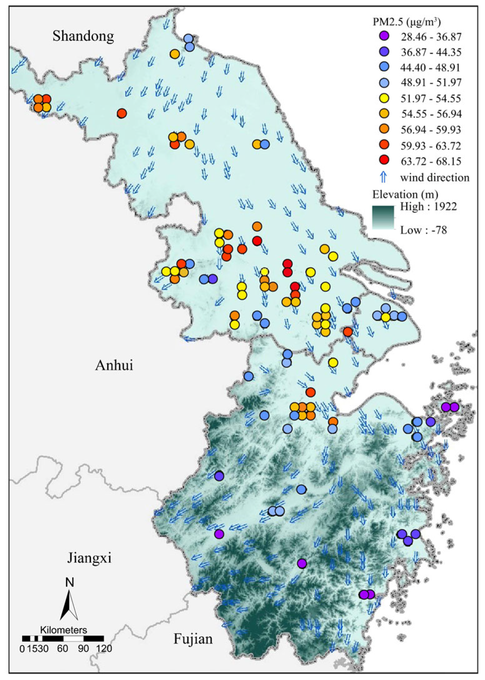
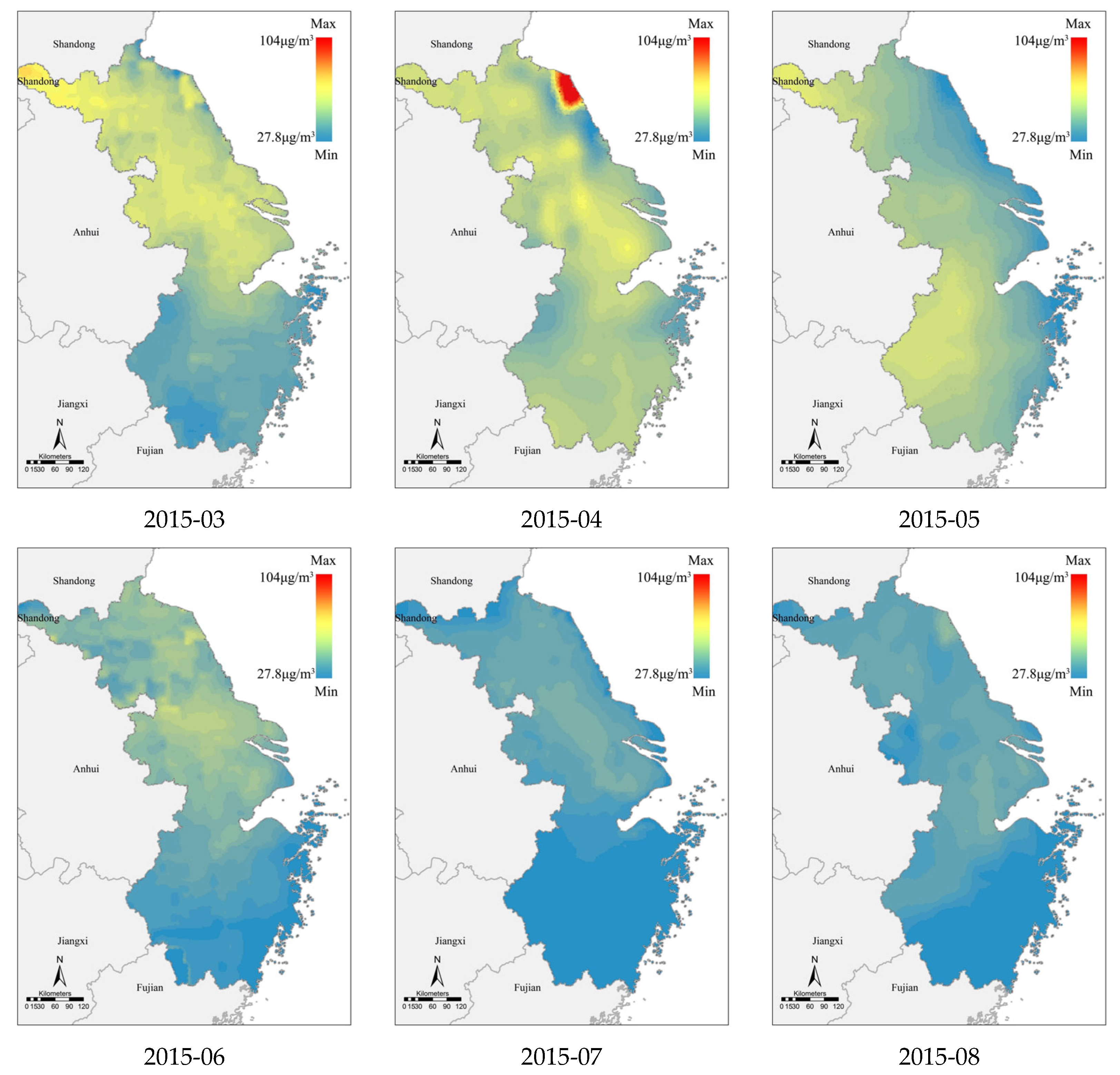
3.5. Results of Full PM_2.5 Estimation with the GDWR Model

The GDWR model was implemented to predict the spatial distribution of the PM_2.5 concentration in the Yangtze River Delta region, and the predicted values are inversely corrected based on the above equation. The spatial resolution is 10 km, and the total data include 2570 grid points. Spatial analysis of the data was carried out from March 2015 to February 2016, as shown in Figure 12. The figure reveals that the PM_2.5 concentration in the Yangtze River Delta region exhibits significant seasonal and cyclical characteristics. According to the monthly analysis, the PM_2.5 concentration decreases starting in March 2015 and reaches its lowest level in July. Thereafter, it increases and peaks in December. An overall decline is observed based on the continuous decrease. According to the seasonal analysis, the summer PM_2.5 concentrations are the lowest, the winter PM_2.5 concentrations are the highest, and the spring and autumn concentrations are the transition periods of the PM_2.5 concentration.

In addition, the PM_2.5 concentration in the Yangtze River Delta region shows significant spatial variation characteristics consistent with the relevant literature [46,47,48], with monthly averages showing an overall decreasing trend from Jiangsu to Zhejiang, with the characteristics of high in the north and low in the south.

4. Conclusions

The PM_2.5 concentration has significant non-stationarity. In previous studies, spatial non-stationarity was widely examined and addressed, and PM_2.5 exhibited a strong directional non-stationarity due to its wind diffusion characteristics. Studies that consider the wind influence on PM_2.5 estimation have been carried out; however, they lacked the quantitative and fundamental combination of directional and spatial non-stationarity, which may further limit accuracy improvement. By breaking through the traditional isotropy spatial field assumption, constructing the space distance model directionally constrained by the wind field, this study first combined spatial and directional non-stationarity on PM_2.5 concentration estimation and proposed the geographically directionally weighted regression model (GDWR).

To assess the efficacy of our method, monthly PM_2.5 concentration estimation was carried out as a case study from March 2015 to February 2016 in the Yangtze River Delta region. The results indicate that the GDWR model attained the best fitting effect (0.79) and the smallest error fluctuation, the OLS model yielded the worst fitting effect (0.589), and the GWR (0.72) and DWR (0.74) fitting effects were moderate. Non-stationarity hypothesis testing was conducted to objectively confirm the occurrence of directional non-stationarity. Based on time series data of the PM_2.5 concentration, we determined the influence of wind field changes on the propagation, diffusion, and dissipation of PM_2.5 in the different seasons. The GDWR model proposed in this study provides a certain guiding significance for the estimation and analysis of similar geographical elements with directional propagation characteristics.

References

1. ISO. Air quality–Particle size fraction definitions for health-related sampling. In ISO 7708; ISO: Geneva, Switzerland, 1995. [Google Scholar]
2. Boldo, E.; Medina, S.; LeTertre, A.; Hurley, F.; Mücke, H.; Ballester, F.; Aguilera, I.; Eilstein, D.; Group, A. Apheis: Health impact assessment of long-term exposure to PM(2.5) in 23 European cities. Eur. J. Epidemiol. 2006, 21, 449–458. [Google Scholar] [CrossRef] [PubMed]
3. Watterson, T.; Sorensen, J.; Martin, R.; Coulombe, R.A., Jr. Effects of PM2.5 Collected from Cache Valley Utah on Genes Associated with the Inflammatory Response in Human Lung Cells. J. Toxicol. Environ. Health 2007, 70, 1731–1744. [Google Scholar] [CrossRef]
4. Evans, J.; van Donkelaar, A.; Martin, R.V.; Burnett, R.; Rainham, D.G.; Birkett, N.J.; Krewski, D. Estimates of global mortality attributable to particulate air pollution using satellite imagery. Environ. Res. 2013, 120, 33–42. [Google Scholar] [CrossRef]
5. Liu, Y.; Koutrakis, P.; Kahn, R. Estimating fine particulate matter component concentrations and size distributions using satellite-retrieved fractional aerosol optical depth: Part 2-A case study. J. Air Waste Manag. Assoc. 2007, 57, 1360–1369. [Google Scholar] [CrossRef]
6. Zhang, Y.; Cao, F. Fine particulate matter (PM2.5) in China at a city level. Sci. Rep. 2015, 5, 14884. [Google Scholar] [CrossRef] [Green Version]
7. Hoff, R.M.; Christopher, S.A. Remote Sensing of Particulate Pollution from Space: Have We Reached the Promised Land? J. Air Waste Manag. Assoc. 2009, 59, 645–675. [Google Scholar] [CrossRef]
8. van Donkelaar, A.; Martin, R.V.; Brauer, M.; Kahn, R.; Levy, R.; Verduzco, C.; Villeneuve, P.J. Global Estimates of Ambient Fine Particulate Matter Concentrations from Satellite-Based Aerosol Optical Depth: Development and Application. Environ. Health Perspect. 2010, 118, 847–855. [Google Scholar] [CrossRef] [PubMed] [Green Version]
9. Kumar, N.; Chu, A.; Foster, A. An empirical relationship between PM2.5 and aerosol optical depth in Delhi Metropolitan. Atmos. Environ. 2007, 41, 4492–4503. [Google Scholar] [CrossRef] [Green Version]
10. Kahn, R.; Banerjee, P.; McDonald, D. Sensitivity of multiangle imaging to natural mixtures of aerosols over ocean. J. Geophys. Res. Atmos. 2001, 106, 18219–18238. [Google Scholar] [CrossRef] [Green Version]
11. Kahn, R.; Banerjee, P.; McDonald, D.; Diner, D.J. Sensitivity of multiangle imaging to aerosol optical depth and to pure-particle size distribution and composition over ocean: The Earth Observing System (EOS) AM-1 platform. J. Geophys. Res. 1998, 103, 32195–32213. [Google Scholar] [CrossRef]
12. Liu, Y.; Park, R.J.; Jacob, D.J.; Li, Q.; Kilaru, V.; Sarnat, J.A. Mapping annual mean ground-level PM2.5 concentrations using Multiangle Imaging Spectroradiometer aerosol optical thickness over the contiguous United States. J. Geophys. Res. Atmos. 2004, 109, D22206. [Google Scholar]
13. Yu, S.; Mathur, R.; Schere, K.; Kang, D.; Pleim, J.; Young, J.; Tong, D.; Pouliot, G.; McKeen, S.A.; Rao, S.T. Evaluation of real-time PM2.5 forecasts and process analysis for PM2.5 formation over the eastern United States using the Eta-CMAQ forecast model during the 2004 ICARTT study. J. Geophys. Res. Atmos. 2008, 113, D06204. [Google Scholar] [CrossRef] [Green Version]
14. San Jose, R.; Pérez, J.L.; Morant, J.L.; González, R.M. Elevated PM10 and PM2.5 Concentrations in Europe: A Model Experiment with MM5-CMAQ and WRF-CHEM; WIT: Southampton, UK, 2008. [Google Scholar]
15. Saide, P.E.; Carmichael, G.R.; Spak, S.; Gallardo, L. Forecasting urban PM10 and PM2.5 pollution episodes in very stable nocturnal conditions and complex terrain using WRF–Chem CO tracer model. Atmos. Environ. 2011, 45, 2769–2780. [Google Scholar] [CrossRef]
16. Chu, D.A.; Kaufman, Y.J.; Zibordi, G.; Chern, J. Global monitoring of air pollution over land from the Earth Observing System-Terra Moderate Resolution Imaging Spectroradiometer (MODIS). J. Geophys. Res. Atmos. 2003, 108, 4661. [Google Scholar] [CrossRef]
17. Engel-Cox, J.A.; Holloman, C.H.; Coutant, B.W.; Hoff, R.M. Qualitative and quantitative evaluation of MODIS satellite sensor data for regional and urban scale air quality. Atmos. Environ. 2004, 38, 2495–2509. [Google Scholar] [CrossRef]
18. Li, C.; Hsu, N.C.; Tsay, S. A study on the potential applications of satellite data in air quality monitoring and forecasting. Atmos. Environ. 2011, 45, 3663–3675. [Google Scholar] [CrossRef]
19. He, Q.; Huang, B. Satellite-based mapping of daily high-resolution ground PM2.5 in China via space-time regression modeling. Remote Sens. Environ. 2018, 206, 72–83. [Google Scholar] [CrossRef]
20. Alexeeff, S.E.; Schwartz, J.; Kloog, I.; Chudnovsky, A.; Koutrakis, P.; Coull, B.A. Consequences of kriging and land use regression for PM2.5 predictions in epidemiologic analyses: Insights into spatial variability using high-resolution satellite data. J. Expo. Sci. Environ. Epidemiol. 2015, 25, 138–144. [Google Scholar] [CrossRef] [Green Version]
21. Gupta, P.; Christopher, S.A. Particulate matter air quality assessment using integrated surface, satellite, and meteorological products: 2. A neural network approach. J. Geophys. Res. Atmos. 2009, 114. [Google Scholar] [CrossRef]
22. Zhang, H.; Hoff, R.M.; Engel-Cox, J.A. The Relation between Moderate Resolution Imaging Spectroradiometer (MODIS) Aerosol Optical Depth and PM2.5 over the United States: A Geographical Comparison by U.S. Environmental Protection Agency Regions. J. Air Waste Manag. Assoc. 2009, 59, 1358–1369. [Google Scholar] [CrossRef] [Green Version]
23. Brunsdon, C.; Fotheringham, S.; Charlton, M. Geographically weighted regression-modelling spatial non-stationarity. J. R. Stat. Soc. Ser. D Stat. 1998, 47, 431–443. [Google Scholar] [CrossRef]
24. Hu, Z. Spatial analysis of MODIS aerosol optical depth, PM2.5, and chronic coronary heart disease. Int. J. Health Geogr. 2009, 8, 27. [Google Scholar] [CrossRef] [Green Version]
25. Ma, Z.; Hu, X.; Huang, L.; Bi, J.; Liu, Y. Estimating Ground-Level PM2.5 in China Using Satellite Remote Sensing. Environ. Sci. Technol. 2014, 48, 7436–7444. [Google Scholar] [CrossRef]
26. Hu, Z.; Liebens, J.; Rao, K.R. Merging Satellite Measurement with Ground-Based Air Quality Monitoring Data to Assess Health Effects of Fine Particulate Matter Pollution; Springer: Dordrecht, The Netherlands, 2011; pp. 395–409. [Google Scholar]
27. Song, W.; Jia, H.; Huang, J.; Zhang, Y. A satellite-based geographically weighted regression model for regional PM2.5 estimation over the Pearl River Delta region in China. Remote Sens. Environ. 2014, 154, 1–7. [Google Scholar] [CrossRef]
28. Huang, B.; Wu, B.; Barry, M. Geographically and temporally weighted regression for modeling spatio-temporal variation in house prices. Int. J. Geogr. Inf. 2010. [Google Scholar] [CrossRef]
29. Seaman, N.L. Meteorological modeling for air-quality assessments. Atmos. Environ. 2000, 34, 2231–2259. [Google Scholar] [CrossRef]
30. Fotheringham, A.S.; Pitts, T.C. Directional variation in distance decay. Environ. Plan. A 1995, 27, 715–729. [Google Scholar] [CrossRef]
31. Jammalamadaka, S.R.; Lund, U.J. The effect of wind direction on ozone levels: A case study. Environ. Ecol. Stat. 2006, 13, 287–298. [Google Scholar] [CrossRef] [Green Version]
32. Lu, H.; Fang, G. Estimating the frequency distributions of PM10 and PM2.5 by the statistics of wind speed at Sha-Lu, Taiwan. Sci. Total. Environ. 2002, 298, 119–130. [Google Scholar] [CrossRef]
33. Soggiu, M.E.; Inglessis, M.; Gagliardi, R.V.; Settimo, G.; Marsili, G.; Notardonato, I.; Avino, P. PM10 and PM2.5 Qualitative Source Apportionment Using Selective Wind Direction Sampling in a Port-Industrial Area in Civitavecchia, Italy. Atmosphere 2020, 11, 94. [Google Scholar] [CrossRef] [Green Version]
34. Zhang, T.; Zhu, Z.; Gong, W.; Zhu, Z.; Sun, K.; Wang, L.; Huang, Y.; Mao, F.; Shen, H.; Li, Z.; et al. Estimation of ultrahigh resolution PM2.5 concentrations in urban areas using 160 m Gaofen-1 AOD retrievals. Remote Sens. Environ. 2018, 216, 91–104. [Google Scholar] [CrossRef]
35. Oller, R.; Martori, J.C.; Madariaga, R. Monocentricity and Directional Heterogeneity: A Conditional Parametric Approach. Geogr. Anal. 2017, 49, 343–361. [Google Scholar] [CrossRef]
36. Li, L.; Gong, J.; Zhou, J. Spatial interpolation of fine particulate matter concentrations using the shortest wind-field path distance. PLoS ONE 2014, 9, e96111. [Google Scholar] [CrossRef] [Green Version]
37. Li, J.; Fan, Z.; Deng, M. A Method of Spatial Interpolation of Air Pollution Concentration Considering Wind Direction and Speed. J. Geo Inf. Sci. 2017, 19, 382–389. [Google Scholar]
38. Koelemeijer, R.B.A.; Homan, C.D.; Matthijsen, J. Comparison of spatial and temporal variations of aerosol optical thickness and particulate matter over Europe. Atmos. Environ. 2006, 40, 5304–5315. [Google Scholar] [CrossRef]
39. Tian, J.; Chen, D. A semi-empirical model for predicting hourly ground-level fine particulate matter (PM2.5) concentration in southern Ontario from satellite remote sensing and ground-based meteorological measurements. Remote Sens. Environ. 2010, 114, 221–229. [Google Scholar] [CrossRef]
40. Barnes, W.L.; Pagano, T.S.; Salomonson, V.V. Prelaunch characteristics of the Moderate Resolution Imaging Spectroradiometer (MODIS) on EOS-AM1. IEEE Trans. Geosci. Remote Sens. 1998, 36, 1088–1100. [Google Scholar] [CrossRef] [Green Version]
41. Remer, L.A.; Kaufman, Y.J.; Tanré, D.; Mattoo, S. The MODIS aerosol algorithm, products, and validation. J. Atmos. Sci. 2005, 62, 947–973. [Google Scholar] [CrossRef] [Green Version]
42. Tao, M.; Wang, J.; Li, R.; Wang, L.; Wang, L.; Wang, Z.; Tao, J.; Che, H.; Chen, L. Performance of MODIS high-resolution MAIAC aerosol algorithm in China: Characterization and limitation. Atmos. Environ. 2019, 213, 159–169. [Google Scholar] [CrossRef]
43. Levy, R.; Hsu, C. MODIS Atmosphere L2 Aerosol Product. In NASA MODIS Adaptive Processing System; Goddard Space Flight Center: Greenbelt, MD, USA, 2015. [Google Scholar]
44. Fotheringham, A.S.; Charlton, M.E.; Brunsdon, C. Geographically Weighted Regression: A Natural Evolution of the Expansion Method for Spatial Data Analysis. Environ. Plan. A 1998, 30, 1905–1927. [Google Scholar] [CrossRef]
45. Hurvich, C.M.; Simonoff, J.S.; Tsai, C. Smoothing parameter selection in nonparametric regression using an improved Akaike information criterion. J. R. Stat. Soc. B 1998, 60, 271–293. [Google Scholar] [CrossRef]
46. Leung, Y.; Mei, C.L.; Zhang, W.X. Statistical tests for spatial nonstationarity based on the geographically weighted regression model. Environ. Plan. A 2000, 32, 9–32. [Google Scholar] [CrossRef]
47. Abdullah, M. Evaluating Particulate Matter 2.5 in the Yangtze River Delta; Missouri State University: Springfield, MO, USA, 2020. [Google Scholar]
48. Mao, W.L.; Xu, J.H.; Lu, D.B.; Yang, D.Y.; Zhao, J.N. An analysis of the spatial-temporal pattern and influencing fctors of PM2.5 in the yangtze river delta in 2015. Resour. Environ. Yangtze Basin 2017, 26, 264–272. [Google Scholar]
Figure 1. Study area, PM2.5 monitoring stations, and the wind fields with their annual mean values. Annual averages are calculated from PM2.5 monitoring values and wind field data for the period March 2015 to February 2016, which are provided by the China Environmental Monitoring Station and European Centre for Medium-Range Weather Forecasts, respectively.
Ijgi 10 00413 g001
Figure 2. Monthly AOD data coverage in study area (2015/03–2016/02); the change in pixel color from black to white indicates the increasing value of AOD, and red pixels indicate missing value.
Ijgi 10 00413 g002aIjgi 10 00413 g002b
Figure 3. Continuous wind field in the research area during the four seasons: (a) spring, (b) summer, (c) autumn, and (d) winter; (e) shows wind rose diagrams illustrating wind direction and wind speed for four seasons.
Ijgi 10 00413 g003aIjgi 10 00413 g003b
Figure 4. Computational workflow of data processing. Input data include text, raster, and vector formats, with the following processing: (1) input data need to be directionally extracted to omit other information from original format (data extraction), and converted to a uniform format (format conversion, for Esri geodatabase) and coordinate system (projection transformation, for EPSG 4549); (2) integrate these data into a unified 10 × 10 km2 grid system on a spatial scale (clip analysis, spatial resample) and unify monthly slices on a temporal scale (temporal resample).
Ijgi 10 00413 g004
Figure 5. The representation of a directionally weighted kernel function in the sample space [35].
Ijgi 10 00413 g005
Figure 6. Distance equation considering the wind influence between starting pixel and destination pixel: (1) first calculate the distance between adjacent grids ( A , B ) , referring to the LVA distance calculation; (2) calculate the distance between dissociative grids (starting, destination), referring to Dijkstra’s shortest path algorithm.
Ijgi 10 00413 g006
Figure 7. Representation of weighted kernel function in wind field space (b): (a) spatially constrained, (c) directionally and spatially constrained [35].
Ijgi 10 00413 g007
Figure 8. Comparison of the monthly model fitting accuracy among the OLS, DWR, GWR, and GDWR models.
Ijgi 10 00413 g008
Figure 9. Scatter plot between corrected measured and corrected fitted PM2.5 concentrations for model fitting.
Ijgi 10 00413 g009
Figure 10. Scatter plot between corrected measured and corrected fitted PM2.5 concentrations for model fitting grouping by corrected measured PM2.5: (a) 0~200 μm, (b) 200~400 μm, (c) 400~600 μm.
Ijgi 10 00413 g010aIjgi 10 00413 g010b
Figure 11. The error of the four models in each station in the whole year.
Ijgi 10 00413 g011aIjgi 10 00413 g011b
Figure 12. Monthly PM2.5 concentration in the research area (GDWR 2015/03–2016/02).
Ijgi 10 00413 g012aIjgi 10 00413 g012b