
Expert Knowledge as Basis for Assessing an Automatic Matching Procedure


Abstract
1. Introduction
1.1. Automatic Matching as a Solution to PAA Procedures
1.2. Research Approach
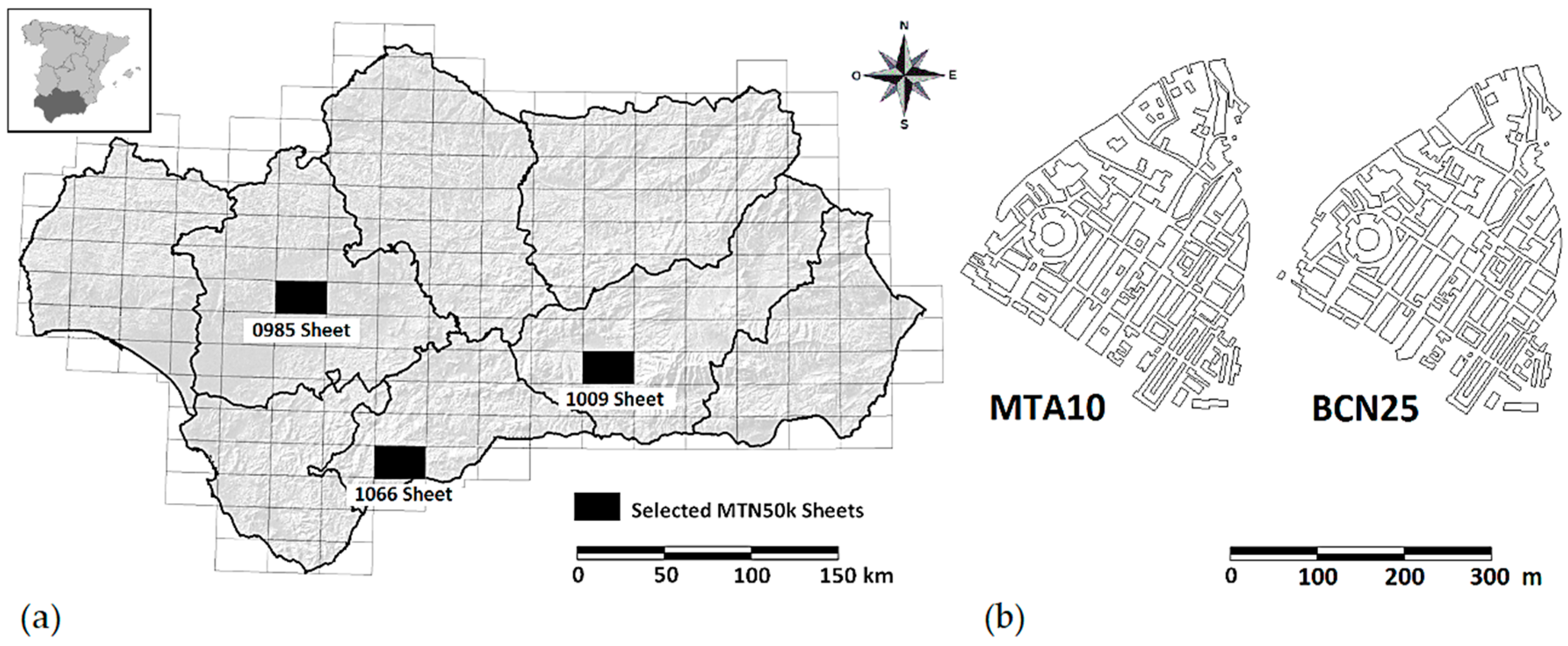
2. Materials and Methods
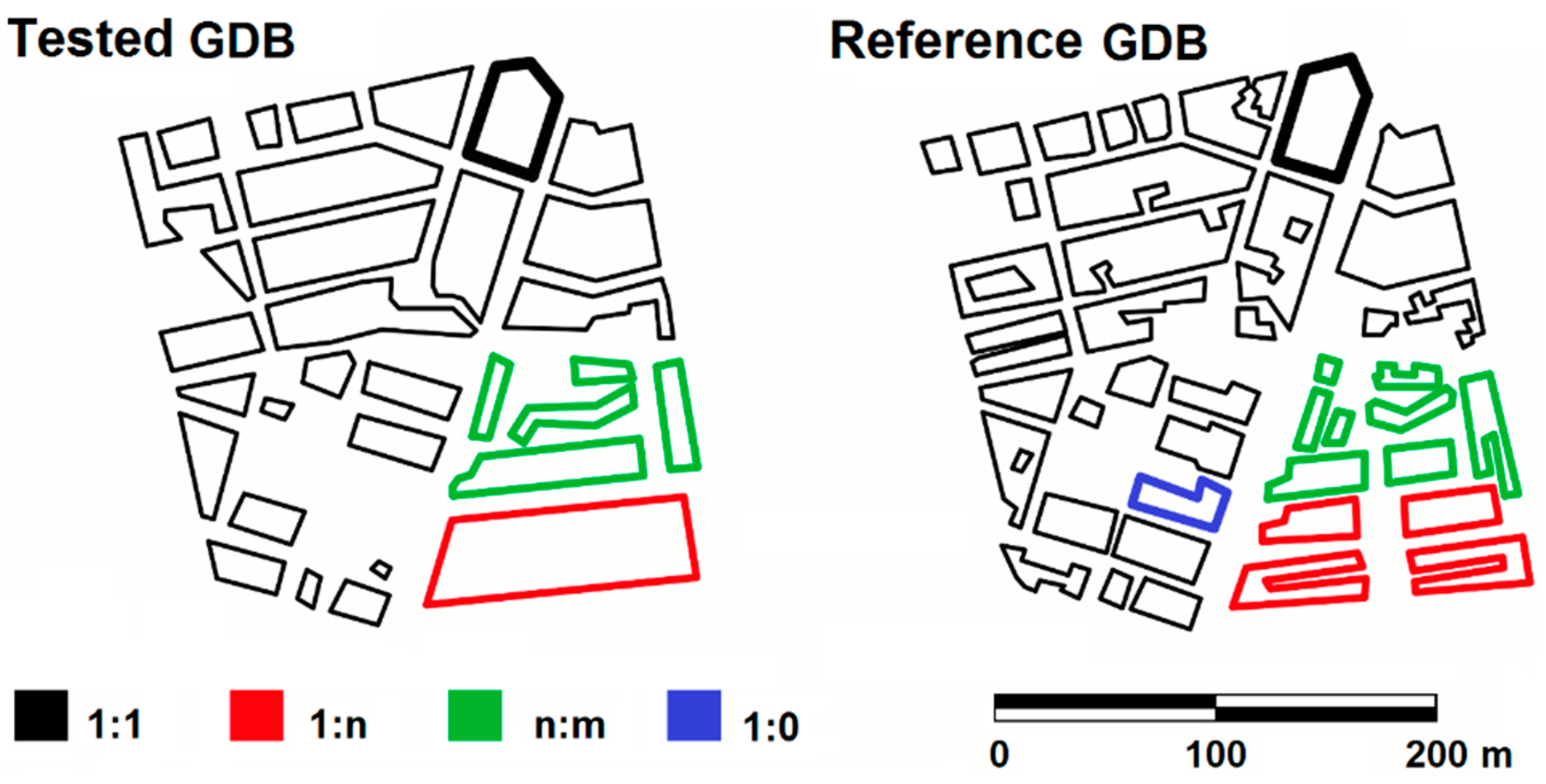
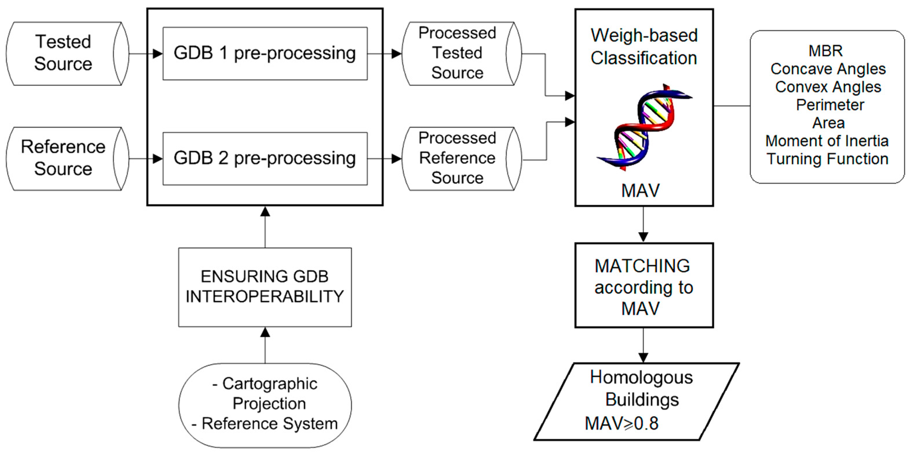
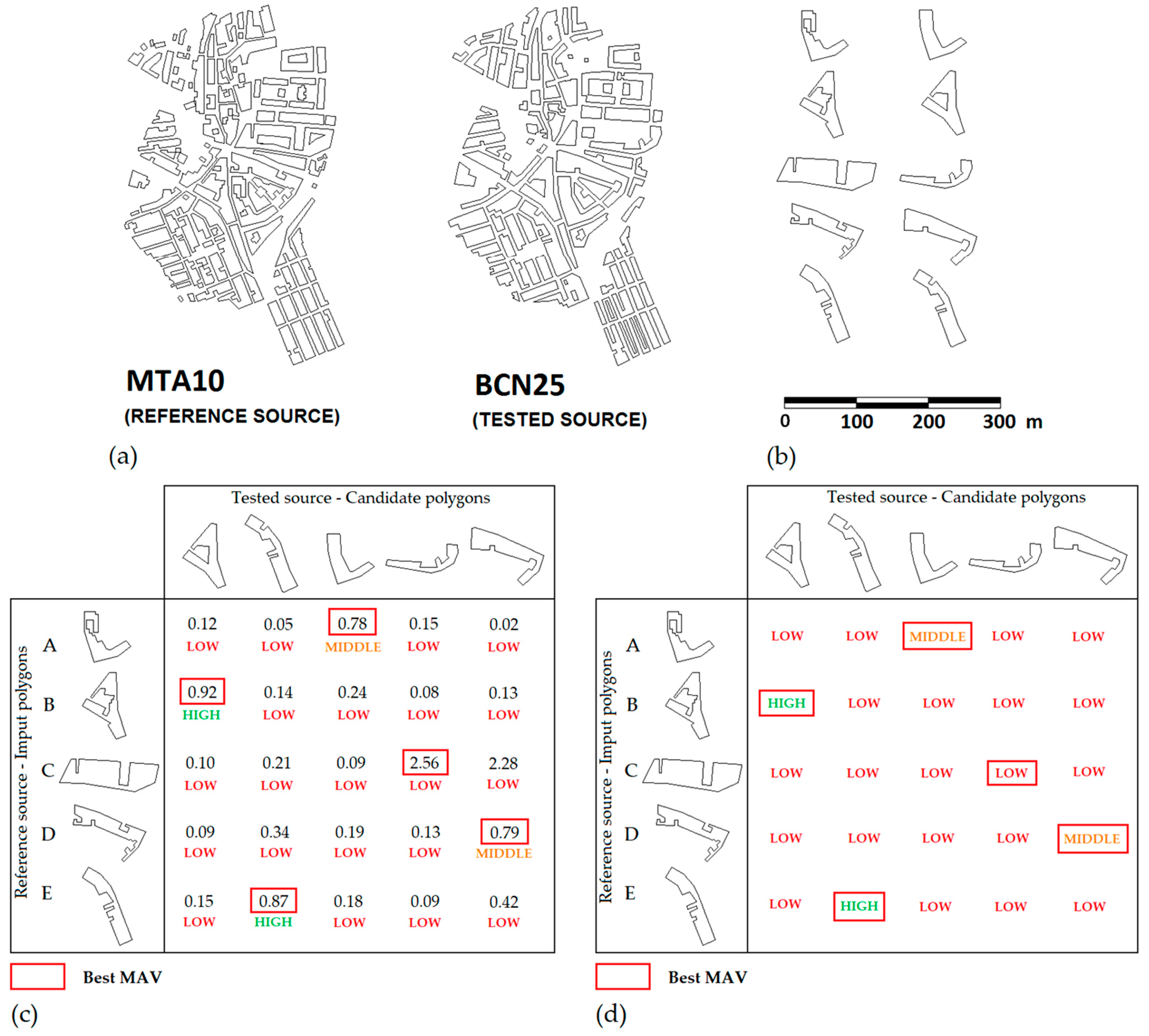
2.1. Automatic Matching Process by Means of a GA
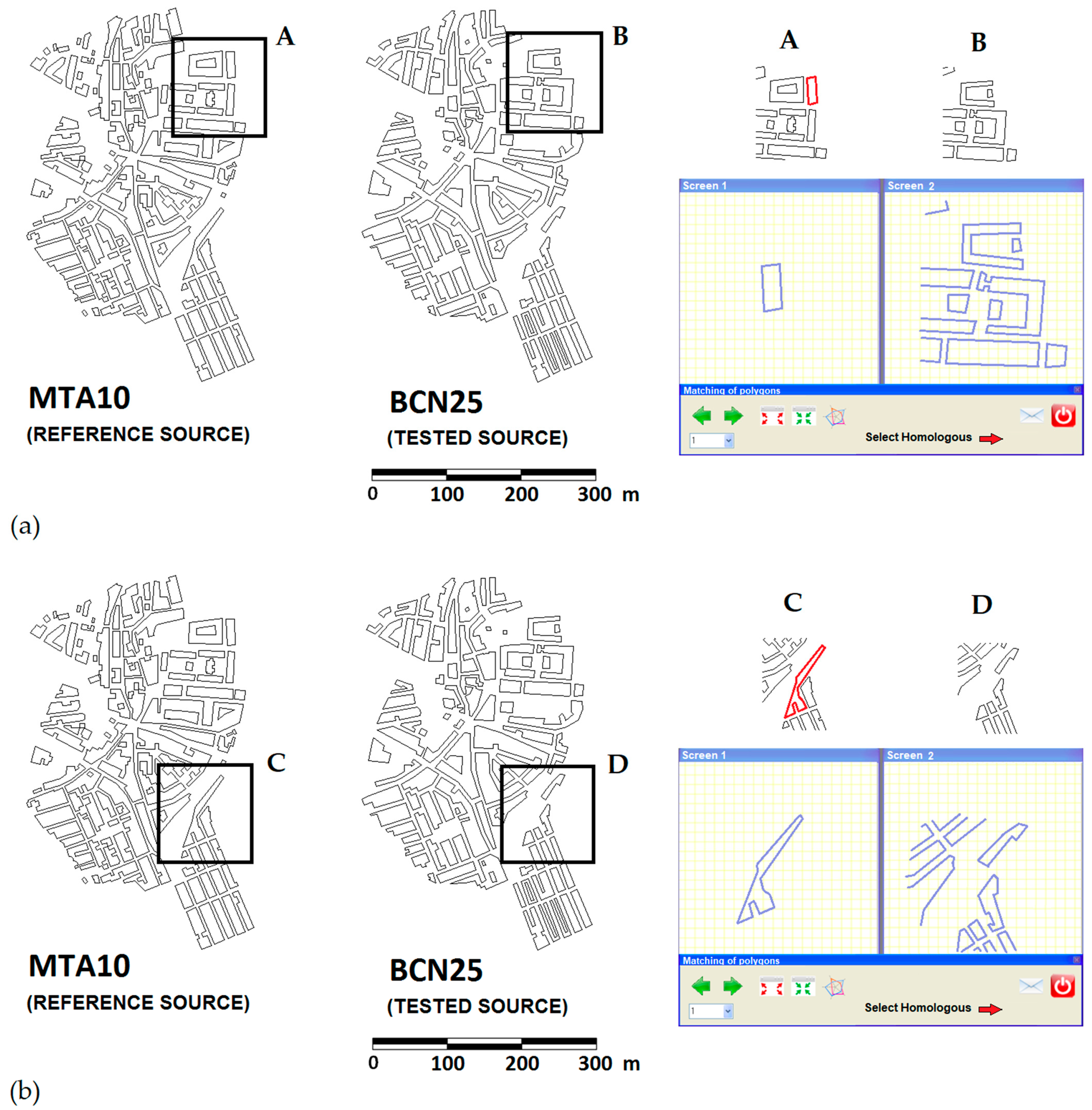
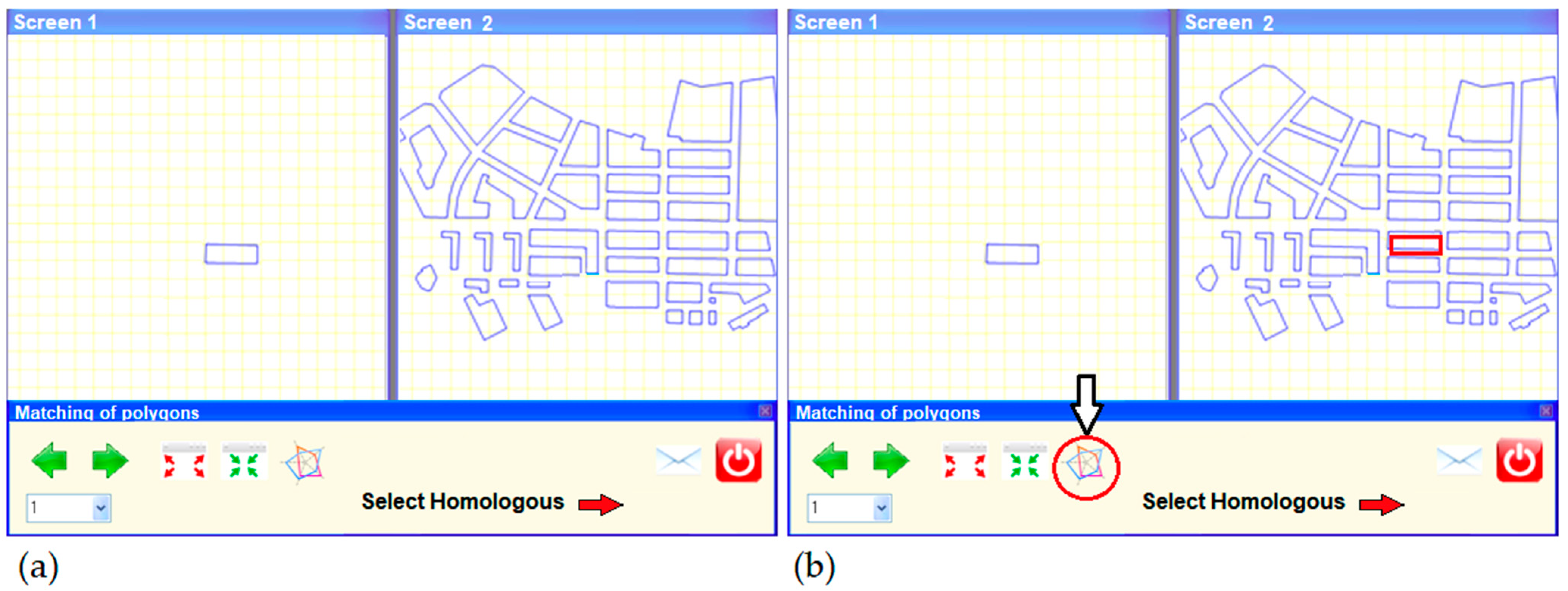
2.2. Manual Matching Carried Out by an Expert Group
- Level of agreement. Defined as the degree of similarity between the judgments issued independently by the different experts;
- Consistency. Defined as the degree of similarity between the judgments issued by the experts and the results provided by the automatic matching process (GA).
2.2.1. Objectives of the Comparison Process
- Provide an alternative MAV (expert value) to the MAV provided by the GA assessing the similarity between building polygons;
- Provide an alternative element matching to those provided by the GA assessing the level of effectiveness of the automatic matching process.
2.2.2. Selection of the Group of Experts
2.2.3. Working Framework and Documentation Provided
- Simultaneous multiple access so that all experts can enter into the application at any time;
- Access restriction. This restriction was established at two different levels: (i) access restriction to any other type of information or software stored in the host computer—with any another way of working, this information would be totally exposed; and (ii) access restriction to the user accounts of other experts.
2.2.4. Design of the Experiments
MAV Experiment
Matching Experiment
Experimental Design
3. Results
3.1. Results Derived from the MAV Experiment
3.2. Results Derived from the Matching Experiment
4. Discussion
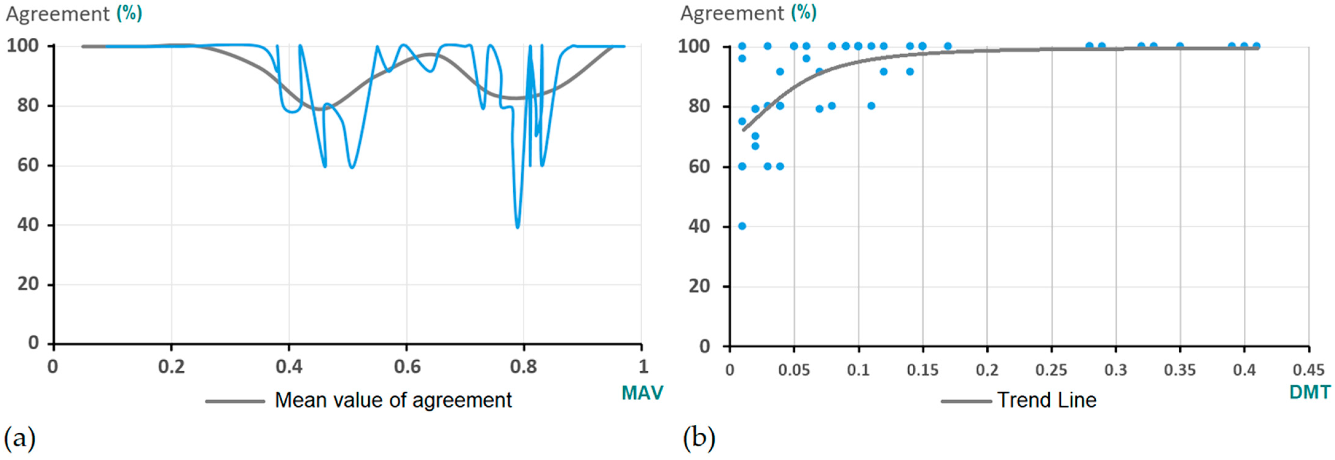
4.1. MAV Experiment
- Polygon number 1. This polygon reached 100% agreement in test number 1, while in the number 4 it did not reach 80% (79.1%).
- Polygon number 4. In this case, the level of agreement reached decreased from 100% (test 1) to 91.6% (test 4).
- Something similar happened with polygons number 48 and 49. Both reached 100% agreement in test number 3, while in test number 4 they dropped to less than 80%.
4.2. Matching Experiment
- Polygon number 31. This polygon reached 100% agreement in test number 2, while in test number 4 it did not reach 87.5%.
- Polygon number 52, whose level of agreement remained constant in tests 3 and 4. In addition, this case reached the lowest agreement level (79.1%) in test number 4. This polygon belongs to the polygons´ typology described above, that is to say, polygons with a square or rectangular shape for which is advisable to employ the edition tools. As stated, the fact that the experts 2, 5, 7, 9 and 11 were not able to match it might be due to a failure to follow the guidelines established by the matching guide.
5. Conclusions
Author Contributions
Funding
Institutional Review Board Statement
Informed Consent Statement
Data Availability Statement
Acknowledgments
Conflicts of Interest
Appendix A

| Test 1 | Test 2 | Test 3 | Test 4 | ||||||||
|---|---|---|---|---|---|---|---|---|---|---|---|
| Pol. | MAV Computed/Discreticed | Pol. | MAV Computed/Discreticed | Pol. | MAV Computed/Discreticed | Pol. | MAV Computed/Discreticed | ||||
| 1 | 0.82/2 | High | 19 | 0.17/0 | Low | 37 | 0.83/2 | High | 1 | 0.82/2 | High |
| 2 | 0.51/1 | Medium | 20 | 0.46/0 | Low | 38 | 0.09/0 | Low | 4 | 0.38/0 | Low |
| 3 | 0.71/1 | Medium | 21 | 0.39/0 | Low | 39 | 0.10/0 | Low | 5 | 0.55/1 | Medium |
| 4 | 0.38/0 | Low | 22 | 0.88/2 | High | 40 | 0.81/2 | High | 6 | 0.74/1 | Medium |
| 5 | 0.55/1 | Medium | 23 | 0.81/2 | High | 41 | 0.15/0 | Low | 7 | 0.86/2 | High |
| 6 | 0.76/1 | Medium | 24 | 0.70/1 | Medium | 42 | 0.57/1 | Medium | 8 | 0.11/0 | Low |
| 7 | 0.86/2 | High | 25 | 0.22/0 | Low | 43 | 0.90/2 | High | 22 | 0.88/2 | High |
| 8 | 0.11/0 | Low | 26 | 0.64/1 | Medium | 44 | 0.66/1 | Medium | 23 | 0.81/2 | High |
| 9 | 0.79/1 | Medium | 27 | 0.83/2 | High | 45 | 0.76/1 | Medium | 25 | 0.22/0 | Low |
| 10 | 0.83/2 | High | 28 | 0.49/0 | Low | 46 | 0.95/2 | High | 26 | 0.64/1 | Medium |
| 11 | 0.91/2 | High | 29 | 0.90/2 | High | 47 | 0.95/2 | High | 28 | 0.49/0 | Low |
| 12 | 0.89/2 | High | 30 | 0.60/1 | Medium | 48 | 0.38/0 | Low | 31 | 0.78/1 | Medium |
| 13 | 0.42/0 | Low | 31 | 0.78/1 | Medium | 49 | 0.78/1 | Medium | 43 | 0.90/2 | High |
| 14 | 0.59/1 | Medium | 32 | 0.46/0 | Low | 50 | 0.81/2 | High | 44 | 0.66/1 | Medium |
| 15 | 0.18/0 | Low | 33 | 0.97/2 | High | 51 | 0.42/0 | Low | 48 | 0.38/0 | Low |
| 16 | 0.90/2 | High | 34 | 0.82/2 | High | 52 | 0.35/0 | Low | 49 | 0.78/1 | Medium |
| 17 | 0.21/0 | Low | 35 | 0.73/1 | Medium | 53 | 0.70/1 | Medium | 50 | 0.81/2 | High |
| 18 | 0.22/0 | Low | 36 | 0.74/1 | Medium | 54 | 0.55/1 | Medium | 52 | 0.35/0 | Low |
| Test 1 | Test 2 | Test 3 | |||||||||||||||||||||
|---|---|---|---|---|---|---|---|---|---|---|---|---|---|---|---|---|---|---|---|---|---|---|---|
| Pol ID. | GA | Expert ID. | Agreement [%] | Pol ID. | GA | Expert ID. | Agreement [%] | Pol ID. | GA | Expert ID. | Agreement [%] | ||||||||||||
| 16 | 5 | 2 | 21 | 8 | 12 | 9 | 1 | 14 | 15 | 3 | 4 | 7 | 6 | 24 | |||||||||
| 1 | 2 | 2 | 2 | 2 | 2 | 2 | 100 | 19 | 0 | 0 | 0 | 0 | 0 | 0 | 100 | 37 | 2 | 2 | 2 | 2 | 2 | 2 | 100 |
| 2 | 1 | 0 | 1 | 1 | 1 | 0 | 60 | 20 | 0 | 1 | 0 | 0 | 1 | 0 | 60 | 38 | 0 | 0 | 0 | 0 | 0 | 0 | 100 |
| 3 | 1 | 1 | 1 | 1 | 1 | 1 | 100 | 21 | 0 | 0 | 1 | 0 | 0 | 0 | 80 | 39 | 0 | 0 | 0 | 0 | 0 | 0 | 100 |
| 4 | 0 | 0 | 0 | 0 | 0 | 0 | 100 | 22 | 2 | 2 | 2 | 2 | 2 | 2 | 100 | 40 | 2 | 1 | 2 | 2 | 1 | 2 | 60 |
| 5 | 1 | 1 | 1 | 1 | 1 | 1 | 100 | 23 | 2 | 2 | 2 | 2 | 2 | 2 | 100 | 41 | 0 | 0 | 0 | 0 | 0 | 0 | 100 |
| 6 | 1 | 2 | 1 | 1 | 1 | 1 | 80 | 24 | 1 | 1 | 1 | 1 | 1 | 1 | 100 | 42 | 1 | 1 | 1 | 1 | 1 | 1 | 100 |
| 7 | 2 | 2 | 2 | 2 | 2 | 2 | 100 | 25 | 0 | 0 | 0 | 0 | 0 | 0 | 100 | 43 | 2 | 2 | 2 | 2 | 2 | 2 | 100 |
| 8 | 0 | 0 | 0 | 0 | 0 | 0 | 100 | 26 | 1 | 1 | 1 | 1 | 1 | 1 | 100 | 44 | 1 | 1 | 1 | 1 | 1 | 1 | 100 |
| 9 | 1 | 1 | 2 | 2 | 1 | 2 | 40 | 27 | 2 | 2 | 2 | 2 | 2 | 2 | 100 | 45 | 1 | 1 | 1 | 2 | 1 | 1 | 80 |
| 10 | 2 | 2 | 2 | 1 | 2 | 2 | 80 | 28 | 0 | 0 | 0 | 1 | 0 | 0 | 80 | 46 | 2 | 2 | 2 | 2 | 2 | 2 | 100 |
| 11 | 2 | 1 | 2 | 2 | 2 | 2 | 100 | 29 | 2 | 2 | 2 | 2 | 2 | 2 | 100 | 47 | 2 | 2 | 2 | 2 | 2 | 2 | 100 |
| 12 | 2 | 2 | 2 | 2 | 2 | 2 | 100 | 30 | 1 | 1 | 1 | 1 | 1 | 1 | 100 | 48 | 0 | 0 | 0 | 0 | 0 | 0 | 100 |
| 13 | 0 | 0 | 1 | 0 | 0 | 0 | 80 | 31 | 1 | 1 | 1 | 2 | 1 | 1 | 80 | 49 | 1 | 1 | 1 | 1 | 1 | 1 | 100 |
| 14 | 1 | 2 | 1 | 1 | 1 | 1 | 100 | 32 | 0 | 0 | 0 | 0 | 0 | 0 | 100 | 50 | 2 | 2 | 2 | 2 | 2 | 2 | 100 |
| 15 | 0 | 0 | 0 | 0 | 0 | 0 | 100 | 33 | 2 | 2 | 2 | 2 | 2 | 2 | 100 | 51 | 0 | 0 | 0 | 0 | 0 | 0 | 100 |
| 16 | 2 | 3 | 2 | 2 | 2 | 2 | 100 | 34 | 2 | 2 | 2 | 2 | 2 | 1 | 80 | 52 | 0 | 0 | 0 | 0 | 0 | 0 | 100 |
| 17 | 0 | 0 | 0 | 0 | 0 | 0 | 100 | 35 | 1 | 2 | 1 | 1 | 1 | 1 | 80 | 53 | 1 | 1 | 1 | 1 | 1 | 1 | 100 |
| 18 | 0 | 0 | 0 | 0 | 0 | 0 | 100 | 36 | 1 | 1 | 1 | 1 | 1 | 1 | 100 | 54 | 1 | 1 | 1 | 1 | 1 | 1 | 100 |
| Test 4 | ||||||||||||||||||||||||||
|---|---|---|---|---|---|---|---|---|---|---|---|---|---|---|---|---|---|---|---|---|---|---|---|---|---|---|
| Pol ID. | GA | Expert ID. | Agreement [%] | |||||||||||||||||||||||
| 1 | 2 | 3 | 4 | 5 | 6 | 7 | 8 | 9 | 10 | 11 | 12 | 13 | 14 | 15 | 16 | 17 | 18 | 19 | 20 | 21 | 22 | 23 | 24 | |||
| 1 | 2 | 2 | 2 | 1 | 2 | 2 | 2 | 1 | 2 | 2 | 1 | 2 | 2 | 2 | 2 | 2 | 2 | 1 | 1 | 2 | 2 | 2 | 2 | 2 | 2 | 79.1 |
| 4 | 0 | 0 | 0 | 0 | 1 | 0 | 0 | 0 | 1 | 0 | 0 | 0 | 0 | 0 | 0 | 0 | 0 | 0 | 0 | 0 | 0 | 0 | 0 | 0 | 0 | 91.6 |
| 5 | 1 | 1 | 1 | 1 | 1 | 1 | 1 | 1 | 1 | 1 | 1 | 1 | 1 | 1 | 1 | 1 | 1 | 1 | 1 | 1 | 1 | 1 | 1 | 1 | 1 | 100 |
| 6 | 1 | 1 | 1 | 1 | 1 | 1 | 1 | 1 | 2 | 1 | 1 | 1 | 1 | 1 | 1 | 1 | 2 | 1 | 1 | 1 | 1 | 1 | 1 | 1 | 1 | 91.6 |
| 7 | 2 | 2 | 2 | 2 | 2 | 2 | 2 | 1 | 2 | 2 | 2 | 2 | 2 | 2 | 2 | 2 | 2 | 2 | 2 | 2 | 2 | 2 | 2 | 2 | 2 | 95.8 |
| 8 | 0 | 0 | 0 | 0 | 0 | 0 | 0 | 0 | 0 | 0 | 0 | 0 | 0 | 0 | 0 | 0 | 0 | 0 | 0 | 0 | 0 | 0 | 0 | 0 | 0 | 100 |
| 22 | 2 | 2 | 2 | 2 | 2 | 2 | 2 | 2 | 2 | 2 | 2 | 2 | 2 | 2 | 2 | 2 | 2 | 2 | 2 | 2 | 2 | 2 | 2 | 2 | 2 | 100 |
| 23 | 2 | 2 | 2 | 2 | 2 | 2 | 2 | 2 | 2 | 2 | 2 | 2 | 2 | 2 | 2 | 2 | 2 | 2 | 2 | 2 | 2 | 2 | 2 | 2 | 2 | 100 |
| 25 | 0 | 0 | 0 | 0 | 0 | 0 | 0 | 0 | 0 | 0 | 0 | 0 | 0 | 0 | 0 | 0 | 0 | 0 | 0 | 0 | 0 | 0 | 0 | 0 | 0 | 100 |
| 26 | 1 | 1 | 1 | 1 | 1 | 1 | 1 | 1 | 1 | 1 | 1 | 0 | 1 | 1 | 1 | 1 | 0 | 1 | 1 | 1 | 1 | 1 | 1 | 1 | 1 | 91.6 |
| 28 | 0 | 1 | 1 | 0 | 0 | 0 | 1 | 1 | 0 | 0 | 0 | 0 | 0 | 0 | 0 | 0 | 0 | 0 | 1 | 0 | 1 | 0 | 0 | 0 | 0 | 75 |
| 31 | 1 | 2 | 2 | 1 | 1 | 1 | 1 | 1 | 1 | 1 | 1 | 1 | 1 | 1 | 1 | 2 | 1 | 1 | 2 | 1 | 1 | 2 | 1 | 1 | 1 | 79.1 |
| 43 | 2 | 2 | 2 | 2 | 2 | 2 | 2 | 2 | 2 | 2 | 2 | 2 | 2 | 2 | 2 | 2 | 2 | 2 | 2 | 2 | 2 | 2 | 2 | 2 | 2 | 100 |
| 44 | 1 | 1 | 1 | 1 | 1 | 1 | 1 | 1 | 1 | 1 | 1 | 1 | 1 | 1 | 1 | 1 | 1 | 1 | 1 | 1 | 1 | 1 | 1 | 1 | 1 | 100 |
| 48 | 0 | 0 | 0 | 0 | 0 | 0 | 0 | 0 | 0 | 1 | 1 | 0 | 0 | 0 | 0 | 1 | 0 | 1 | 0 | 0 | 0 | 0 | 0 | 0 | 0 | 83.3 |
| 49 | 1 | 1 | 2 | 1 | 1 | 2 | 1 | 1 | 1 | 1 | 1 | 1 | 1 | 1 | 2 | 2 | 2 | 1 | 2 | 1 | 1 | 1 | 2 | 2 | 1 | 66.7 |
| 50 | 2 | 1 | 2 | 2 | 2 | 2 | 2 | 2 | 2 | 2 | 2 | 2 | 2 | 2 | 2 | 2 | 2 | 1 | 2 | 2 | 2 | 2 | 2 | 2 | 2 | 95.8 |
| 52 | 0 | 0 | 0 | 0 | 0 | 0 | 0 | 0 | 0 | 0 | 0 | 0 | 0 | 0 | 0 | 0 | 0 | 0 | 0 | 0 | 0 | 0 | 0 | 0 | 0 | 100 |
| Test 1 | Test 2 | Test 3 | Test 4 | ||||
|---|---|---|---|---|---|---|---|
| Pol. ID. | Matched Polygon ID. | Pol. ID. | Matched Polygon ID. | Pol. ID. | Matched polygon ID. | Pol. ID. | Matched Polygon ID. |
| 1 | 247 | 19 | 286 | 37 | 312 | 1 | 247 |
| 2 | 113 | 20 | 236 | 38 | 251 | 4 | 252 |
| 3 | 27 | 21 | 176 | 39 | 87 | 8 | 283 |
| 4 | 252 | 22 | 88 | 40 | 73 | 9 | Unmatched |
| 5 | 231 | 23 | 130 | 41 | 204 | 10 | 133 |
| 6 | 33 | 24 | Unmatched | 42 | 250 | 13 | Unmatched |
| 7 | Unmatched | 25 | 153 | 43 | 140 | 22 | 88 |
| 8 | 283 | 26 | 258 | 44 | 22 | 26 | 258 |
| 9 | Unmatched | 27 | 14 | 45 | 276 | 27 | 14 |
| 10 | 133 | 28 | 114 | 46 | 47 | 28 | 114 |
| 11 | 128 | 29 | Unmatched | 47 | 43 | 31 | 304 |
| 12 | 89 | 30 | 208 | 48 | 61 | 32 | Unmatched |
| 13 | Unmatched | 31 | 304 | 49 | 108 | 43 | 140 |
| 14 | 172 | 32 | Unmatched | 50 | 313 | 44 | 22 |
| 15 | 188 | 33 | 319 | 51 | 214 | 49 | 108 |
| 16 | Unmatched | 34 | 225 | 52 | 191 | 50 | 313 |
| 17 | 285 | 35 | 316 | 53 | 230 | 52 | 191 |
| 18 | 36 | 36 | 154 | 54 | 106 | 53 | 230 |
| Test 1 | Test 2 | Test 3 | |||||||||||||||||||||
|---|---|---|---|---|---|---|---|---|---|---|---|---|---|---|---|---|---|---|---|---|---|---|---|
| Pol ID. | GA | Expert ID. | Agreement [%] | Pol ID. | GA | Expert. ID. | Agreement [%] | Pol ID. | GA | Expert. ID. | Agreement [%] | ||||||||||||
| 16 | 5 | 2 | 21 | 8 | 12 | 9 | 1 | 14 | 15 | 3 | 4 | 7 | 6 | 24 | |||||||||
| 1 | 247 | 247 | 247 | 247 | 247 | 247 | 100 | 19 | 286 | 286 | 286 | 286 | 286 | 286 | 100 | 37 | 312 | 312 | 312 | 312 | 312 | 312 | 100 |
| 2 | 113 | 113 | 113 | 113 | 113 | 113 | 100 | 20 | 236 | 236 | 236 | 236 | 236 | 236 | 100 | 38 | 251 | 251 | 251 | 251 | 251 | 251 | 100 |
| 3 | 27 | 27 | 27 | 27 | 27 | 27 | 100 | 21 | 176 | 176 | 176 | 176 | 176 | 176 | 100 | 39 | 87 | 87 | 87 | 87 | 87 | 87 | 100 |
| 4 | 252 | 252 | 252 | 252 | 252 | 252 | 100 | 22 | 88 | 88 | 88 | 88 | 88 | 88 | 100 | 40 | 73 | 73 | 73 | 73 | 73 | 73 | 100 |
| 5 | 231 | 231 | 231 | 231 | 231 | 231 | 100 | 23 | 130 | 130 | 130 | 130 | 130 | 130 | 100 | 41 | 204 | 204 | 204 | 204 | 204 | 204 | 100 |
| 6 | 133 | 133 | 133 | 133 | 133 | 133 | 100 | 24 | - | - | - | - | - | - | 100 | 42 | 250 | 250 | 250 | 250 | 250 | 250 | 100 |
| 7 | - | - | - | - | - | - | 100 | 25 | 153 | 153 | 153 | 153 | 153 | 153 | 100 | 43 | 140 | 140 | 140 | 140 | 140 | 140 | 100 |
| 8 | 283 | 283 | 283 | 283 | 283 | 283 | 100 | 26 | 258 | 258 | 258 | 258 | 258 | 258 | 100 | 44 | 22 | 22 | 22 | 22 | 22 | 22 | 100 |
| 9 | - | - | - | - | 74 | - | 80 | 27 | 14 | 14 | 14 | 14 | 14 | 14 | 100 | 45 | 276 | 276 | 276 | 276 | 276 | 276 | 100 |
| 10 | 133 | 133 | 133 | 133 | 101 | 133 | 80 | 28 | 114 | 114 | 114 | 114 | 114 | 114 | 100 | 46 | 47 | 47 | 47 | 47 | 47 | 47 | 100 |
| 11 | 128 | 128 | 128 | 128 | 128 | 128 | 100 | 29 | - | - | - | - | - | - | 100 | 47 | 43 | 43 | 43 | 43 | 43 | 43 | 100 |
| 12 | 89 | 89 | 89 | 89 | 89 | 89 | 100 | 30 | 208 | 208 | 208 | 208 | 208 | 208 | 100 | 48 | 61 | 61 | 61 | 61 | 61 | 61 | 100 |
| 13 | - | - | - | - | - | - | 100 | 31 | 304 | 304 | 304 | 304 | 304 | 304 | 100 | 49 | 108 | 108 | 108 | 108 | 108 | 108 | 100 |
| 14 | 172 | 172 | 172 | 172 | 172 | 172 | 100 | 32 | - | - | - | - | - | - | 100 | 50 | 313 | 313 | 313 | 313 | 313 | 313 | 100 |
| 15 | 188 | 188 | 188 | 188 | 188 | 188 | 100 | 33 | 319 | 319 | 319 | 319 | 319 | 319 | 100 | 51 | 214 | 214 | 214 | 214 | 214 | 214 | 100 |
| 16 | - | - | - | - | - | - | 100 | 34 | 225 | 225 | 225 | 225 | 225 | 225 | 100 | 52 | 191 | 191 | 191 | - | 191 | 191 | 80 |
| 17 | 285 | 285 | 285 | 285 | 285 | 285 | 100 | 35 | 316 | 316 | 316 | 316 | 316 | 316 | 100 | 53 | 230 | 230 | 230 | 230 | 230 | 230 | 100 |
| 18 | 36 | 36 | 36 | 36 | 36 | 36 | 100 | 36 | 154 | 154 | 154 | 154 | 154 | 154 | 100 | 54 | 106 | 106 | 106 | 106 | 106 | 106 | 100 |
| Test 4 | ||||||||||||||||||||||||||
|---|---|---|---|---|---|---|---|---|---|---|---|---|---|---|---|---|---|---|---|---|---|---|---|---|---|---|
| Pol ID. | GA | Expert ID. | Agreement [%] | |||||||||||||||||||||||
| 1 | 2 | 3 | 4 | 5 | 6 | 7 | 8 | 9 | 10 | 11 | 12 | 13 | 14 | 15 | 16 | 17 | 18 | 19 | 20 | 21 | 22 | 23 | 24 | |||
| 1 | 247 | 247 | 247 | 247 | 247 | 247 | 247 | 247 | 247 | 247 | 247 | 247 | 247 | 247 | 247 | 247 | 247 | 247 | 247 | 247 | 247 | 247 | 247 | 247 | 247 | 100 |
| 4 | 252 | 252 | 252 | 252 | 252 | 252 | 252 | 252 | 252 | 252 | 252 | 252 | 252 | 252 | 252 | 252 | 252 | 252 | 252 | 252 | 252 | 252 | 252 | 252 | 252 | 100 |
| 8 | 283 | 283 | 283 | 283 | 283 | 283 | 283 | 283 | 283 | 283 | 283 | 283 | 283 | 283 | 283 | 283 | 283 | 283 | 283 | 283 | 283 | 283 | 283 | 283 | 283 | 100 |
| 9 | - | - | - | - | - | - | - | - | - | - | - | - | - | - | - | - | - | - | - | - | - | - | - | - | - | 100 |
| 10 | 133 | 133 | 133 | 133 | 133 | 133 | 133 | 133 | 133 | 133 | 133 | - | 133 | 133 | 133 | 133 | 133 | 133 | 133 | 133 | 133 | 101 | 133 | 133 | 133 | 91.6 |
| 13 | - | - | - | - | - | - | - | - | - | - | - | - | - | - | - | - | - | - | - | - | - | - | - | - | - | 100 |
| 22 | 88 | 88 | 88 | 88 | 88 | 88 | 88 | 88 | 88 | 88 | 88 | 88 | 88 | 88 | 88 | 88 | 88 | 88 | 88 | 88 | 88 | 88 | 88 | 88 | 88 | 100 |
| 26 | 258 | 258 | 258 | 258 | 258 | 258 | 258 | 258 | 258 | 258 | 258 | - | 258 | 258 | 258 | 258 | 258 | 258 | 258 | 258 | 258 | 258 | 258 | 258 | 258 | 95.8 |
| 27 | 14 | 14 | 14 | 14 | 14 | 14 | 14 | 14 | 14 | 14 | 14 | 14 | 14 | 14 | 14 | 14 | 14 | 14 | 14 | 14 | 14 | 14 | 14 | 14 | 14 | 100 |
| 28 | 114 | 114 | 114 | 114 | 114 | 114 | 114 | 114 | 114 | 114 | 114 | - | 114 | 114 | 114 | 114 | 114 | 114 | 114 | 114 | 114 | 114 | 114 | 114 | 114 | 95.8 |
| 31 | 304 | 304 | - | 304 | 304 | - | 304 | 304 | 304 | 304 | 304 | - | 304 | 304 | 304 | 304 | 304 | 304 | 304 | 304 | 304 | 304 | 304 | 304 | 304 | 87.5 |
| 32 | - | - | - | - | - | - | - | - | - | - | - | - | - | - | - | - | - | - | - | - | - | - | - | - | - | 100 |
| 43 | 140 | 140 | 140 | 140 | 140 | 140 | 140 | 140 | 140 | 140 | 140 | 140 | 140 | 140 | 140 | 140 | 140 | 140 | 140 | 140 | 140 | 140 | 140 | 140 | 140 | 100 |
| 44 | 22 | 22 | 22 | 22 | 22 | 22 | 22 | 22 | 22 | 22 | 22 | 22 | 22 | 22 | 22 | 22 | 22 | 22 | 22 | 22 | 22 | 22 | 22 | 22 | 22 | 100 |
| 49 | 108 | 108 | 108 | 108 | 108 | 108 | 108 | 108 | 108 | 108 | 108 | 108 | 108 | 108 | 108 | 108 | 108 | 108 | 108 | 108 | 108 | 108 | 108 | 108 | 108 | 100 |
| 50 | 313 | 313 | 313 | 313 | 313 | 313 | 313 | 313 | 313 | 313 | 313 | - | 313 | 313 | 313 | 313 | 313 | 313 | 313 | 313 | 313 | 313 | 313 | 313 | 313 | 95.8 |
| 52 | 191 | 191 | - | 191 | 191 | - | 191 | - | 191 | - | 191 | - | 191 | 191 | 191 | 191 | 191 | 191 | 191 | 191 | 191 | 191 | 191 | 191 | 191 | 79.1 |
| 53 | 230 | 230 | 230 | 230 | 230 | 230 | 230 | 230 | 230 | 230 | 230 | 230 | 230 | 230 | 230 | 230 | 230 | 230 | 230 | 230 | 230 | 230 | 230 | 230 | 230 | 100 |
References
- Ruiz-Lendinez, J.J.; Ureña-Cámara, M.A.; Ariza-López, F.J. A Polygon and Point-Based Approach to Matching Geospatial Features. ISPRS Int. J. Geo-Inf. 2017, 6, 399. [Google Scholar] [CrossRef]
- Fleuret, F.; Li, T.; Dubout, C.; Wampler, E.K.; Yantis, S.; Geman, D. Comparing machines and humans on a visual categorization test. Proc. Natl. Acad. Sci. USA 2011, 108, 17621–17625. [Google Scholar] [CrossRef] [PubMed]
- Hassabis, D.; Kumaran, D.; Summerfield, C.; Botvinick, M. Neuroscience-inspired artificial intelligence. Neuron 2017, 95, 245–258. [Google Scholar] [CrossRef] [PubMed]
- Borowski, J.; Funke, C.; Stosio, K.; Brendel, W.; Wallis, T.; Bethge, M. The Notorious Difficulty of Comparing Human and Machine Perception. In Proceedings of the Conference on Cognitive Computational Neuroscience, Berlin, Germany, 13–16 September 2019. [Google Scholar]
- Nyandwi, E.; Koeva, M.; Kohli, D.; Bennett, R. Comparing Human versus Machine-Driven Cadastral Boundary Feature Extraction. Remote Sens. 2019, 11, 1662. [Google Scholar] [CrossRef]
- Quackenbush, L.J. A Review of Techniques for Extracting Linear Features from Imagery. Photogramm. Eng. Remote Sens. 2004, 70, 1383–1392. [Google Scholar] [CrossRef]
- Krizhevsky, A.; Sutskever, I.; Hinton, G.E. ImageNet classification with deep convolutional neural networks. Adv. Neural Inf. Proc. Syst. 2012, 25, 1097–1105. [Google Scholar] [CrossRef]
- Eigen, D.; Fergus, R. Predicting depth, surface normals and semantic labels with a common multi-scale convolutional architecture. In Proceedings of the IEEE International Conference on Computer Vision, Santiago, Chile, 7–13 December 2015. [Google Scholar]
- Zhang, X.; Zhao, X.; Molenaar, M.; Stoter, J.; Kraak, M.; Tinghua, A. Pattern classification approaches to matching building polygons at multiple scales. In Proceedings of the ISPRS Annals of the Photogrammetry, Remote Sensing and Spatial Information Sciences, Volume I-2, XXII ISPRS Congress, Melbourne, Australia, 25 August–1 September 2012. [Google Scholar]
- Fan, H.; Zipf, A.; Fu, Q.; Neis, P. Quality assessment for building footprints data on OpenStreetMap. Int. J. Geogr. Inf. Sci. 2014, 28, 700–719. [Google Scholar] [CrossRef]
- Tang, J.; Jiang, B.; Zheng, A.; Luo, B. Graph matching based on spectral embedding with missing value. Pattern Recognit. 2012, 45, 3768–3779. [Google Scholar] [CrossRef]
- Feng, W.; Liu, Z.; Wan, L.; Pun, C.; Jiang, J. A spectral-multiplicity-tolerant approach to robust graph matching. Pattern Recognit. 2013, 46, 2819–2829. [Google Scholar] [CrossRef]
- Dold, J.; Groopman, J. Geo-spatial Information Science The future of geospatial intelligence. Future Geospat. Intell. 2017, 20, 5020–5151. [Google Scholar]
- Devogele, T.; Trevisan, J.; Raynal, L. Building a multi-scale database with scale-transition relationships. In Proceedings of the 7th International Symposium on Spatial Data Handling, Delft, The Netherlands, 12–16 August 1996; Taylor & Francis: Oxford, UK, 1996; pp. 337–351. [Google Scholar]
- Yuan, S.; Tao, C. Development of conflation components. In Proceedings of the Geoinformatics’99 Conference, Ann Arbor, MI, USA, 19–21 June 1999; pp. 1–13. [Google Scholar]
- Song, W.; Keller, J.; Haithcoat, T.; Davis, C. Relaxation-Based Point Feature Matching for Vector Map Conflation. Trans. GIS 2011, 15, 43–60. [Google Scholar] [CrossRef]
- Stoter, J.; Burghardt, D.; Duchêne, C.; Baella, B.; Bakker, N.; Blok, C.; Pla, M.; Regnauld, N.; Touya, G.; Schmid, S. Methodology for evaluating automated map generalization in commercial software. Comput. Environ. Urban Syst. 2009, 33, 311–324. [Google Scholar] [CrossRef]
- Ruiz-Lendinez, J.J.; Ariza-López, F.J.; Ureña-Cámara, M.A. Automatic positional accuracy assessment of geospatial databases using line-based methods. Surv. Rev. 2013, 45, 332–342. [Google Scholar] [CrossRef]
- Ruiz-Lendinez, J.J.; Ariza-López, F.J.; Ureña-Cámara, M.A. A point-based methodology for the automatic positional accuracy assessment of geospatial databases. Surv. Rev. 2016, 48, 269–277. [Google Scholar] [CrossRef]
- Goodchild, M.; Hunter, G. A Simple Positional Accuracy Measure for Linear Features. Int. J. Geogr. Inf. Sci. 1997, 11, 299–306. [Google Scholar] [CrossRef]
- Hastings, J.T. Automated conflation of digital gazetteer data. Int. J. Geogr. Inf. Sci. 2008, 22, 1109–1127. [Google Scholar] [CrossRef]
- Huh, Y.; Yu, K.; Heo, J. Detecting conjugate-point pairs for map alignment between two polygon datasets. Comput. Environ. Urban Syst. 2011, 35, 250–262. [Google Scholar] [CrossRef]
- Samal, A.; Seth, S.; Cueto, K. A feature-based approach to conflation of geospatial source. Int. J. Geogr. Inf. Sci. 2004, 18, 459–489. [Google Scholar] [CrossRef]
- Kim, J.; Yu, K.; Heo, J.; Lee, W. A new method for matching objects in two different geospatial datasets based on the geographic context. Comput. Geosci. 2010, 36, 1115–1122. [Google Scholar] [CrossRef]
- Arkin, E.; Chew, L.; Huttenlocher, D.; Kedem, K.; Mitchell, J. An efficiently computable metric for comparing polygonal shapes. IEEE Trans. Pattern Anal. Mach. Intell. 1991, 13, 209–216. [Google Scholar] [CrossRef]
- Olteanu-Raimond, A.; Mustière, S.; Ruas, A. Knowledge formalization for vector data matching using belief theory. J. Spat. Inf. Sci. 2015, 10, 21–46. [Google Scholar] [CrossRef]
- Jones, C.B.; Ware, J.M.; Miller, D.R. A probabilistic approach to environmental change detection with area-class map data. In Integrated Spatial Databases; Agouris, P., Stefanidis, A., Eds.; Springer: Berlin/Heidelberg, Germany, 1999; pp. 122–136. [Google Scholar]
- Herrera, F.; Lozano, M.; Verdegay, J. Tackling Real-Coded Genetic Algorithms: Operators and Tools for Behavioural Analysis. Artif. Intell. Rev. 1998, 12, 265–319. [Google Scholar] [CrossRef]
- Herrera, F.; Lozano, M.; Sánchez, A. A Taxonomy for the Crossover Operator for Real-coded Genetic Algorithms: An Experimental Study. Int. J. Intell. Syst. 2003, 18, 309–338. [Google Scholar] [CrossRef]
- Elder, J.; Zucker, S. The effect of contour closure on the rapid discrimination of two-dimensional shapes. Vis. Res. 1993, 33, 981–991. [Google Scholar] [CrossRef]
- Kovacs, I.; Julesz, B. A closed curve is much more than an incomplete one: Effect of closure in figure-ground segmentation. Proc. Natl. Acad. Sci. USA 1993, 90, 7495–7497. [Google Scholar] [CrossRef] [PubMed]
- Ringach, D.L.; Shapley, R. Spatial and temporal properties of illusory contours and amodal boundary completion. Vis. Res. 1996, 36, 3037–3050. [Google Scholar] [CrossRef]
- Tversky, T.; Geisler, W.S.; Perry, J.S. Contour grouping: Closure effects are explained by good continuation and proximity. Vis. Res. 2004, 44, 2769–2777. [Google Scholar] [CrossRef] [PubMed]
- Ullman, S.; Assif, L.; Fetaya, E.; Harari, D. Atoms of recognition in human and computer vision. Proc. Natl. Acad. Sci. USA 2016, 113, 2744–2749. [Google Scholar] [CrossRef] [PubMed]
- Majaj, N.J.; Pelli, D.G. Deep learning-using machine learning to study biological vision. J. Vis. 2018, 18, 22. [Google Scholar] [CrossRef]
- Kar, K.; Kubilius, J.; Schmidt, K.; Issa, E.B.; DiCarlo, J.J. Evidence that recurrent circuits are critical to the ventral stream’s execution of core object recognition behaviour. Nat. Neurosc. 2019, 22, 974. [Google Scholar] [CrossRef]
- Ruiz-Lendinez, J.J.; Ariza-López, F.J.; Ureña-Cámara, M.A. Study of NSSDA Variability by Means of Automatic Positional Accuracy Assessment Methods. ISPRS Int. J. Geo-Inf. 2019, 8, 552. [Google Scholar] [CrossRef]
- Kuhnert, P.M.; Martin, T.G.; Griffiths, S.P. A guide to eliciting and using expert knowledge in Bayesian ecological models. Ecol. Lett. 2010, 7, 900–914. [Google Scholar] [CrossRef] [PubMed]
- Ayyub, B.M. Elicitation of Expert Opinions for Uncertainty and Risks; CRC Press: Boca Ratón, FL, USA, 2001. [Google Scholar]
- Roberson, C.; Feick, R. Defining Local Experts: Geographical Expertise as a Basis for Geographic Information Quality. In Proceedings of Workshops and Posters at the 13th International Conference on Spatial Information Theory (COSIT 2017); Clementini, E., Fogliaroni, P., Ballatore, A., Eds.; Springer: L’Aquila, Italy, 2017; Article No. 22; pp. 22:1–22:14. [Google Scholar]
- Brodaric, B.; Fox, P.; McGuinness, D.L. Geoscience Knowledge representation in cyber infrastructure. Comput. Geosci. 2009, 35, 697–699. [Google Scholar] [CrossRef]
- Casas, J.; Repullo, J.; Donado, J. La encuesta como técnica de investigación. Elaboración de cuestionarios y tratamiento estadístico de los datos (I). Aten. Primaria 2003, 31, 527–538. [Google Scholar] [CrossRef]
- Fischler, M.; Elschlager, R. The representation and matching of pictorial structures. IEEE Trans. Comput. 1973, 22, 67–92. [Google Scholar] [CrossRef]
- Radoux, J.; Waldner, F.; Bogaert, P. How Response Designs and Class Proportions Affect the Accuracy of Validation Data. Remote Sens. 2020, 12, 257. [Google Scholar] [CrossRef]


Publisher’s Note: MDPI stays neutral with regard to jurisdictional claims in published maps and institutional affiliations. |
© 2021 by the authors. Licensee MDPI, Basel, Switzerland. This article is an open access article distributed under the terms and conditions of the Creative Commons Attribution (CC BY) license (https://creativecommons.org/licenses/by/4.0/).
Share and Cite
Ruiz-Lendínez, J.J.; Ariza-López, F.J.; Ureña-Cámara, M.A. Expert Knowledge as Basis for Assessing an Automatic Matching Procedure. ISPRS Int. J. Geo-Inf. 2021, 10, 289. https://doi.org/10.3390/ijgi10050289
Ruiz-Lendínez JJ, Ariza-López FJ, Ureña-Cámara MA. Expert Knowledge as Basis for Assessing an Automatic Matching Procedure. ISPRS International Journal of Geo-Information. 2021; 10(5):289. https://doi.org/10.3390/ijgi10050289
Chicago/Turabian StyleRuiz-Lendínez, Juan José, Francisco Javier Ariza-López, and Manuel Antonio Ureña-Cámara. 2021. "Expert Knowledge as Basis for Assessing an Automatic Matching Procedure" ISPRS International Journal of Geo-Information 10, no. 5: 289. https://doi.org/10.3390/ijgi10050289
APA StyleRuiz-Lendínez, J. J., Ariza-López, F. J., & Ureña-Cámara, M. A. (2021). Expert Knowledge as Basis for Assessing an Automatic Matching Procedure. ISPRS International Journal of Geo-Information, 10(5), 289. https://doi.org/10.3390/ijgi10050289