Marker-Less UAV-LiDAR Strip Alignment in Plantation Forests Based on Topological Persistence Analysis of Clustered Canopy Cover

Abstract

A holistic strategy is established for automated UAV-LiDAR strip adjustment for plantation forests, based on hierarchical density-based clustering analysis of the canopy cover. The method involves three key stages: keypoint extraction, feature similarity and correspondence, and rigid transformation estimation. Initially, the HDBSCAN algorithm is used to cluster the scanned canopy cover, and the keypoints are marked using topological persistence analysis of the individual clusters. Afterward, the feature similarity is calculated by considering the linear and angular relationships between each point and the pointset centroid. The one-to-one feature correspondence is retrieved by solving the assignment problem on the similarity score function using the Kuhn–Munkres algorithm, generating a set of matching pairs. Finally, 3D rigid transformation parameters are determined by permutations over all conceivable pair combinations within the correspondences, whereas the best pair combination is that which yields the maximum count of matched points achieving distance residuals within the specified tolerance. Experimental data covering eighteen subtropical forest plots acquired from the GreenValley and Riegl UAV-LiDAR platforms in two scan modes are used to validate the method. The results are extremely promising for redwood and poplar tree species from both the Velodyne and Riegl UAV-LiDAR datasets. The minimal mean distance residuals of 31 cm and 36 cm are achieved for the coniferous and deciduous plots of the Velodyne data, respectively, whereas their corresponding values are 32 cm and 38 cm for the Riegl plots. Moreover, the method achieves both higher matching percentages and lower mean distance residuals by up to 28% and 14 cm, respectively, compared to the baseline method, except in the case of plots with extremely low tree height. Nevertheless, the mean planimetric distance residual achieved by the proposed method is lower by 13 cm.

1. Introduction

Forest mapping plays a decisive role in many aspects including mitigating climate change, reconstruction of the ecological environment, and promoting economic development. Both natural and planted forests fulfill these aspects and applications, resulting in a wide range of management practices and ecosystems [1]. Traditional mapping techniques use field measurements, which are time-consuming and thus expensive. In contrast, remote sensing data provide tree information from large-scale projects in a shorter time. The rough terrain and dense canopy render forest mapping challenging to both traditional and developing techniques. Advances in modern remote sensing techniques overcome these challenges owing to the large-scale data collection and the variety of perspectives. Light Detection And Ranging (LiDAR) represents a valuable remote sensing tool for forest mapping, evaluation and inventory calculation, with a variety of platforms, from ground-based to air-based modes. Recently, the evolution of light-weight platforms, such as Unmanned Aerial Vehicles (UAVs) having onboard laser sensors, handheld laser scanners, and Backpack Laser Scanners (BLS), has made them emerging devices in forest planning [2,3,4,5]. In addition to the relatively low cost, light weight, and operational flexibility of the UAV system, the main advantage is the provision of data in a global coordinate frame using an on-board Global Navigation Satellite System and Inertial Measurement Unit (GNSS/IMU) sensors. Moreover, the use of UAVs in forests offers rich information about the canopy structure and provides accurate tree heights. However, the under-canopy structure is scanned at a low density, which is challenging to UAVs in high-density forests [6,7] depending upon the sensor capabilities, especially the LiDAR pulse energy.

The UAV-LiDAR has been widely used in forestry applications due to its relatively low time-cost, large-scale coverage and lower occlusion compared to the ground-based LiDAR platforms. The main feature of the UAV systems is that they provide the data in global coordinate frame thanks to their onboard GNSS/IMU integration, which continuously measures real-time three-dimensional (3D) positions of the platform during flight with limited accuracy [8,9,10,11,12,13,14,15]. To ensure complete coverage and least occlusion in data acquisition, UAV-LiDAR data are acquired in overlapping strips/scans, which in turn allows for data redundancy that is useful in overcoming the navigation system-related errors. 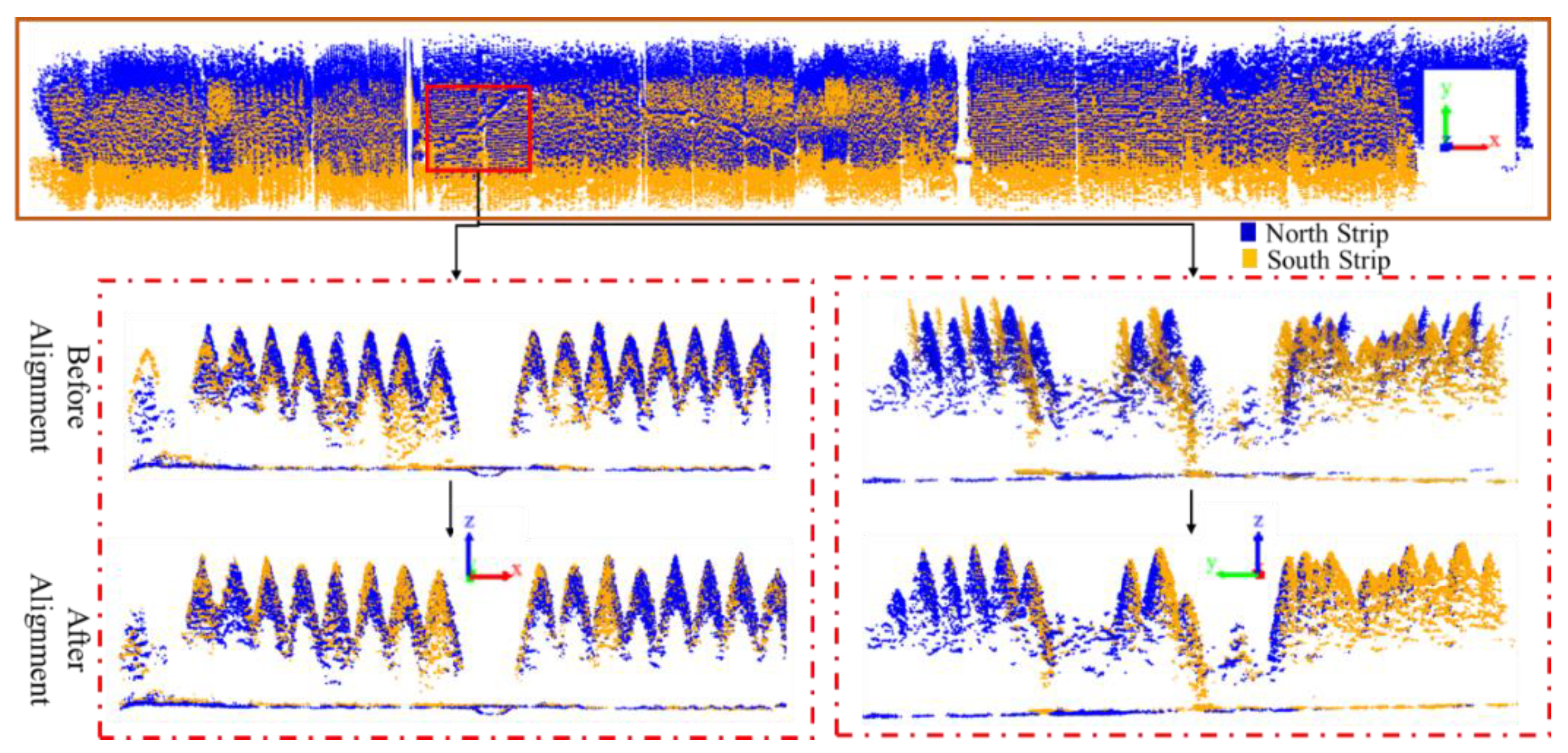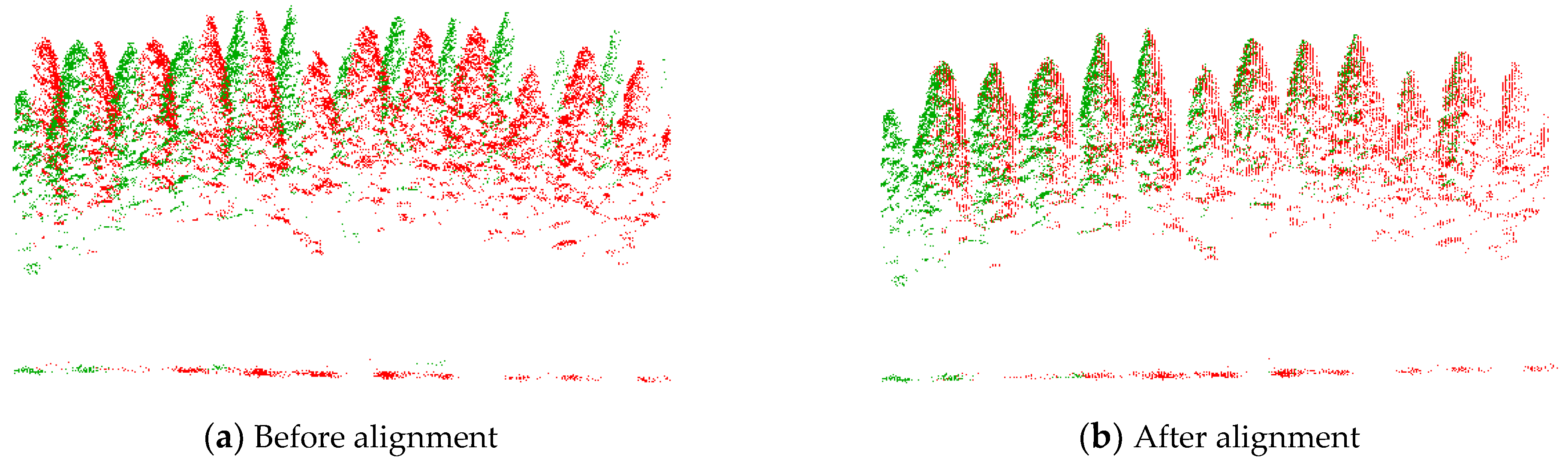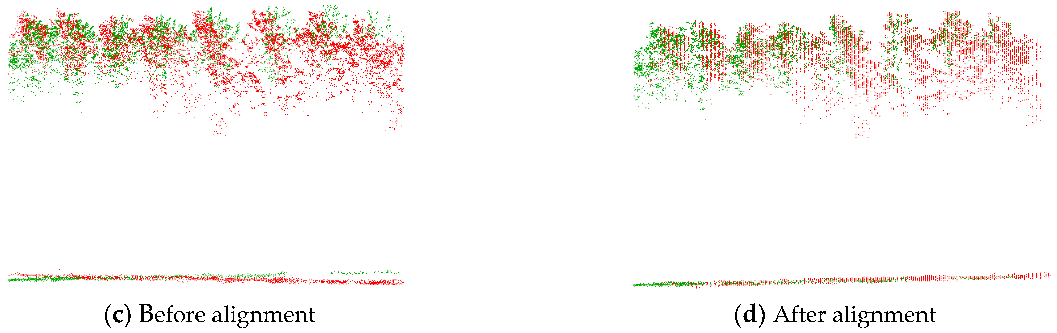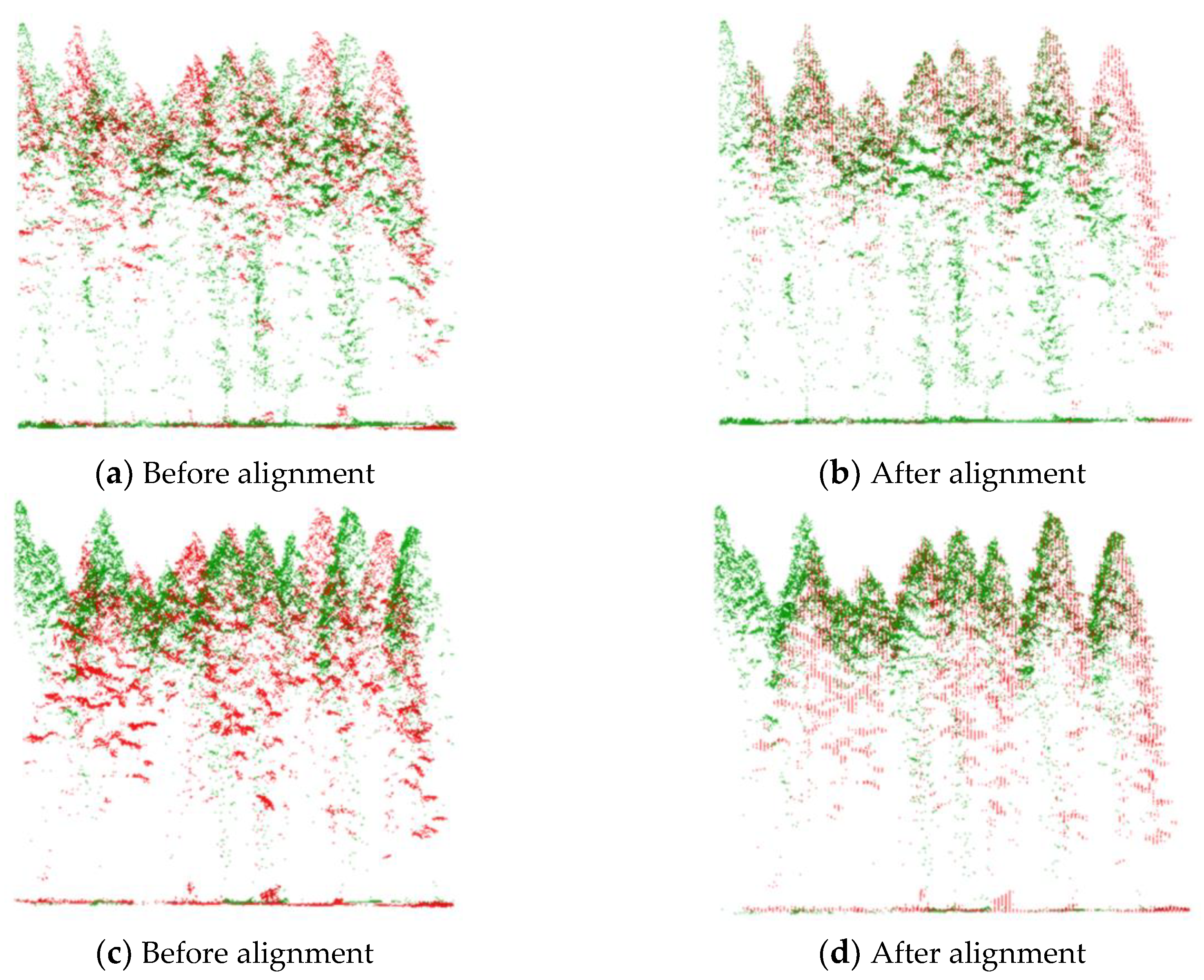These errors are strongly related to the multisensory configuration of UAVs, such as misalignment and gyro drift of the Inertial Navigation System (INS) [16]. This will affect the result of the scan data, especially when merging multiple overlapping scans or strips, as shown in Figure 1. Therefore, the use of an appropriate calibration/adjustment approach is required. The core objective of this calibration process is to eradicate the effects of system-induced errors and provide better analysis of the integrated point clouds, which is referred to as strip adjustment.

The strip adjustment is simply a coordinate transformation process that aims to geometrically refine multiple strips into a unified coordinate frame. This can be done using a set of conjugate points within the strips. Thus, the chief requirement of strip alignment is to identify enough keypoints and a sufficient side overlap between strips. According to these requirements, the process drawbacks are represented in the overlap ratio, the cost of artificial markers, dense forests, and limited feature types in forest scans. The scanned features are exploited to compensate for the lack of Ground Control Points (GCPs) [17]. The available features are related to the type and nature of the scanning project; for example, when working on urban scenes, there are a variety of features (buildings, like-pole objects, road intersections, etc.) that represent different geometries (points, lines, planes, etc.). In contrast, forest scans contain only one feature type represented in the trees, which presents a challenge for feature matching, especially in plantation forest where all trees have approximately the same parameters in both the tree and plot levels. Although much research has been done on marker-free point cloud co-registration in forested areas [18,19,20,21,22,23,24], these mostly use the scanned trees and their parameters as tree location or shape analysis. These approaches are considered here to highlight the problem of feature limitation in forest scans, but not all of them perform strip alignment or work with point clouds from airborne platforms.

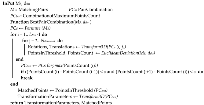
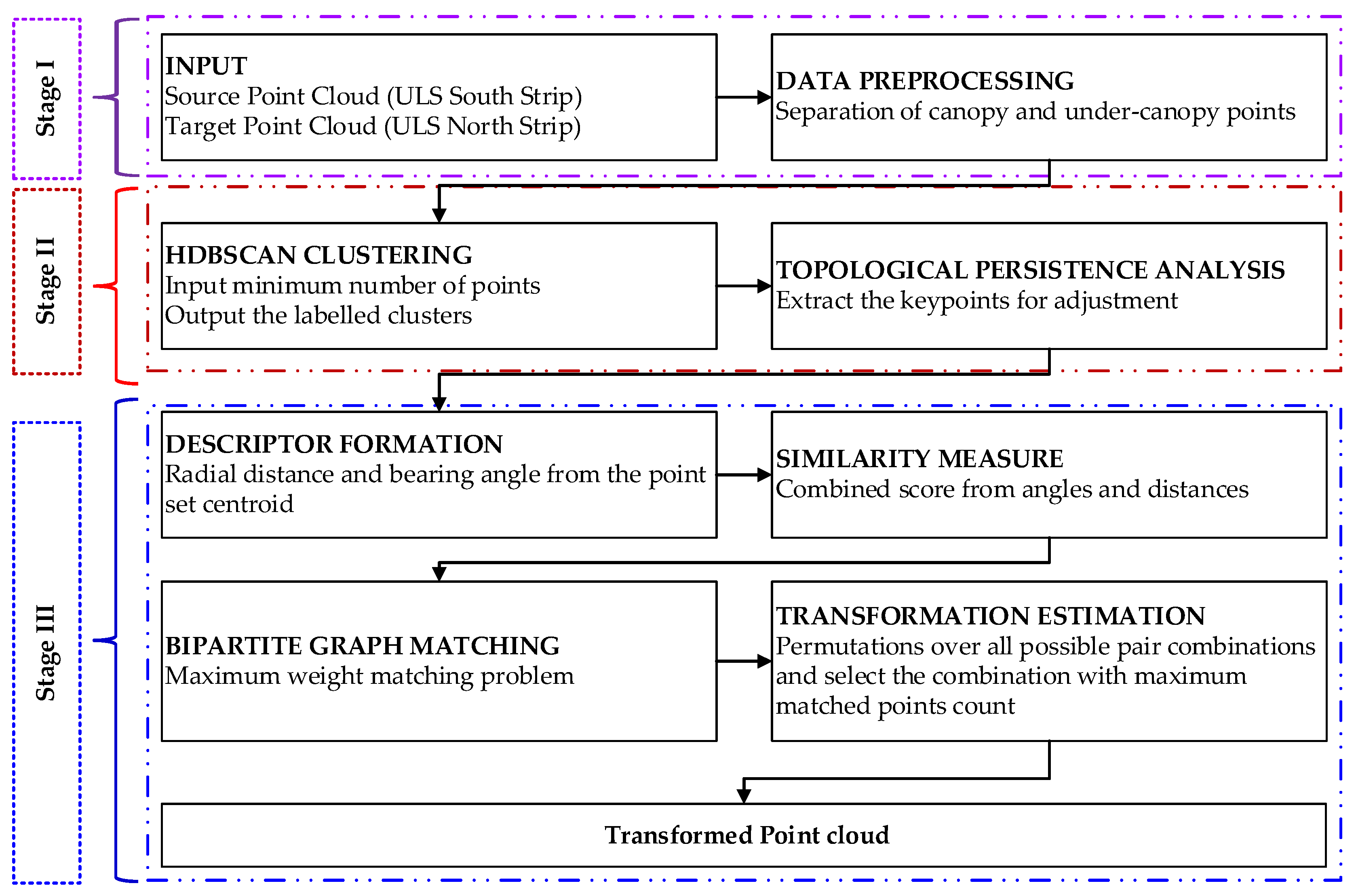
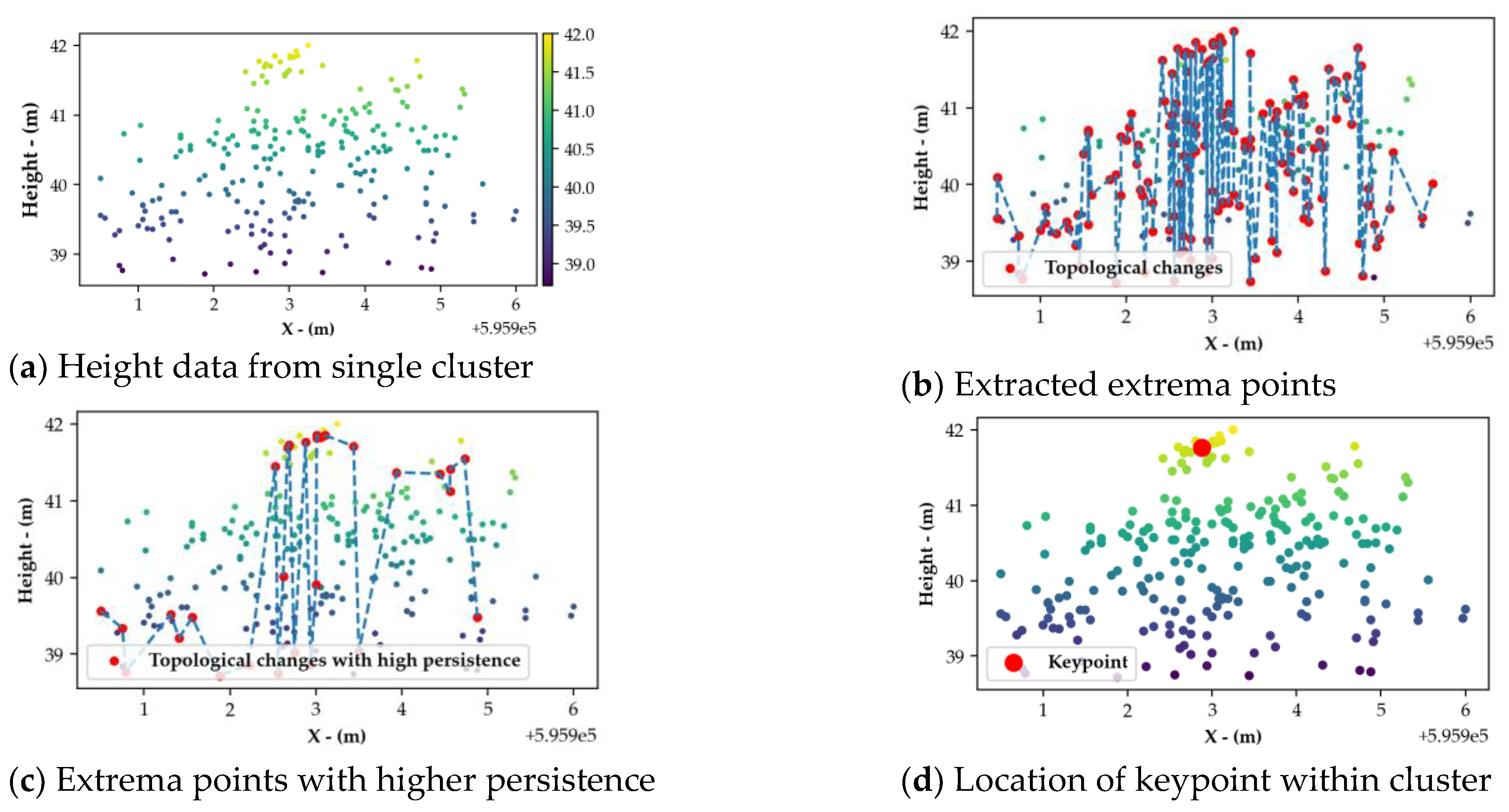
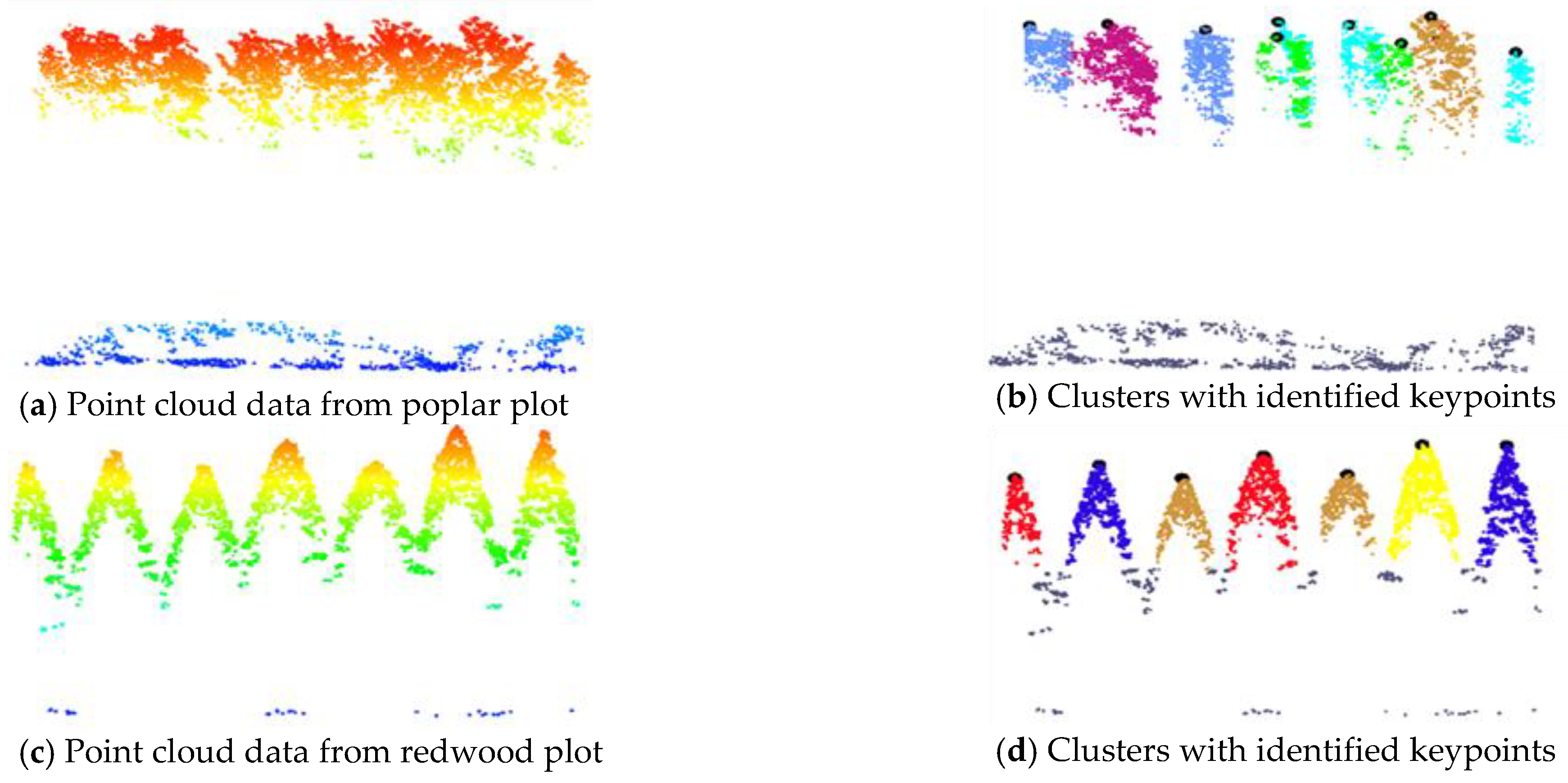
Herein, a generic method is introduced for a UAV-LiDAR strip-wise alignment in forested areas, by clustering the canopy cover using the Hierarchical Density-Based Spatial Clustering of Applications with Noise (HDBSCAN) algorithm and extraction of virtual keypoints from the topological persistence analysis of the resulting individual clusters. This research is a further development and extension of our work [25], in which the UAV-LiDAR strips have been aligned geometrically using the keypoint sets from the canopy clusters resulting from applying Density-Based Spatial Clustering of Applications with Noise (DBSCAN) clustering on the canopy cover. The individual clusters are modeled by Gaussian mixtures and analyzed to define their means, which are used as the keypoints. Each point set is considered a local coordinate frame in which the bearing angle and radial distances from all points and the set centroid are well-defined. The point features are matched via graph matching on the source and target features to obtain one-to-one feature correspondence. The two-dimensional (2D) rigid (one rotation and two translations) coordinate transformations are searched by permuting over all pair combinations to determine the pair that reflects the maximum matching percentage within the specified planimetric distance threshold, while the z-translation is performed separately using the digital elevation model (DEM) values of the matched points. In this work, the method has been expanded with more datasets to include data from two different Pulse Repetition Frequencies (PRFs), accompanied by more experiments. The additional research contributions and innovations over [25] are as follows:

• The 3D transformation parameters are retrieved for direct alignment between the UAV-LiDAR strips without the need for extra information from single tree segmentation, which remains challenging in terms of both performance and accuracy for complex forest stands.
• The advantages of the HDBSCAN algorithm are exploited to cluster the varying density point cloud data.
• The appropriate keypoints are extracted using topological persistence analysis of the individual density-based clusters.
• The permutations over all possible combinations from the correspondence set are used to determine the best pairs combination to calculate 3D rigid transformation with 6 DoF (three rotations and three translations).

The remainder of the paper is organized as follows. The relevant research work is presented in Section 2. Section 3 introduces the study area and the datasets and explains the research methodology. The experimental results and discussion are presented in Section 4 and Section 5. Finally, the conclusions are provided in Section 6.

2. Related Work

The strip adjustment is a major process in photogrammetric projects, whose data are acquired in strips or multiple scans. It aims to geometrically align paired or grouped strips into a unified coordinate frame. The process is performed using either marker-based or marker-free approaches. The marker-based methods are commonly found in commercial software and essentially depend on a set of GCPs that are defined as part of the scanning project. The challenges of the conventional registration method are the availability of the GNSS/IMU to the end-user and the time-cost of establishing GCPs, especially in forest areas. Therefore, the marker-free/marker-less approaches have been developed to overcome these drawbacks. The marker-less approaches are commonly used in literature for urban and forest point clouds simultaneously. On the one hand, the feature diversity in urban scenes allows various point cloud strip alignment and multi-scan co-registration based on points [26,27,28,29], lines [17,30,31,32] and planar surfaces [33,34,35]. On the other hand, several point cloud co-registration approaches have been performed in forested areas using the forest structure, tree parameters and virtual points from tree shape analysis. An object-based method [18] performed Airborne Laser Scanning /Terrestrial Laser Scanning (ALS/TLS) data integration using a heuristic search algorithm to define the optimal point pairs that are retrieved from graph matching, on the similarity score of the feature descriptors formed from the distance relationships between the segmented tree locations within the same forest plot. This work was extended [36] using the co-register UAV/BLS data in the forest through simulated annealing optimization to geometrically align the BLS data to the UAV point cloud in 3D space. The main limitation of this research is that it primarily depends on the accuracy of the extracted tree locations. Guan et al. [37] assumed a common fixed forest geometry between the segmented trees in the point cloud from the UAV, BLS, and TLS and introduced an approach for their co-registration, based on the angle and area matching of the Triangular Irregular Networks (TINs) created between the tree locations in the forest plot. Finally, fine registration was performed via the Iterative Closest Point (ICP) algorithm. The accuracy of this method is mostly affected by tree localization and the existence of whole trees in the scan pairs to be aligned, which is difficult to guarantee when dealing with different acquisition perspectives (e.g., ALS/TLS or UAV/BLS), offering different levels of detail or high-density forests. A method utilizing the canopy analysis [20] applies the mean-shift approach twice to first extract the tree crowns, then searches the individual crown modes that are matched by a probability density function and aligned using the Coherent Point Drift (CPD) algorithm. The method was used to test forest plots from the ALS/TLS combinations. Brede et al. [5] compared the RIEGL VUX-1 UAV system with TLS to derive the canopy height and Diameter at Breast Height (DBH). For the TLS data, automatic registration was performed by extracting tie points depending on the retro-reflective cylinders. Then, they applied a multi-station adjustment to enhance the registration. They obtained a standard deviation of 0.62 cm for the errors for all the tie planes. A method in Paris et al. [22] was implemented to utilize the complementary LiDAR data coverage obtained from diverse viewpoints, specifically ALS and TLS, to accurately describe the 3D structure of individual tree crowns. They exploited correlation images of the aerial and terrestrial Canopy Height Models (CHMs) to estimate the optimum 2D rigid transform (two translations, one rotation).

3. Materials and Methods

3.1. Materials

3.1.1. Study Suite

The Dongtai Forest, located in southeast China on the coast of the Yellow Sea (120.826° E, 32.873° N), as shown in Figure 2a, is considered for this study. It is a planted forest with major tree species including dawn redwood (Metasequoia glyptostroboides), poplar (Populus deltoides), and ginkgo (Ginkgo biloba L.). The total area is approximately 22.4 km², with altitudes ranging from 11 to 14 m above the mean sea level. Figure 2b shows the rectangular vicinity (1500 m × 130 m) outstretched in the west–east direction, encompassing diverse forest parameters and a point cloud view of the eight plots.

UAV strips (each 150 m in width and their lengths are 1500 and 1600 m for the south and north strips) were scanned using a GreenValley UAV system with side lap of 80%. Eight circular test plots with a 50 m diameter were selected within the overlapping area of the strips, in which plots V1, V2, and V4 have poplar (deciduous) trees, and the other plots (V3, V5, V6, V7, and V8) are dawn redwood (coniferous) plots.

Table 1. Forest parameters of the test plots from Velodyne UAV.

Plot Id	Tree Species	Average Tree Height (m)	Stand Density (Tree/ha)
V1	poplar	25.6	333
V2	poplar	21.7	417
V3	dawn redwood	23.6	417
V4	poplar	30.3	208
V5	dawn redwood	7.7	1000
V6	dawn redwood	4.6	417
V7	dawn redwood	6.7	1667
V8	dawn redwood	19.1	1667

lists the forest parameters of the eight plots from the GreenValley UAV-LiDAR.

Another strip pair (with dimensions of 1300 × 80 m), as shown in Figure 2c, within the study area was scanned using a RIEGL UAV VUX-1 laser scanner in two different laser Pulse Repetition Frequencies (PRFs): 380 Hz and 550 Hz. The side overlap was quite low (45%), and consequently, ten forest plots were selected from the overlapping area with a 30 m diameter. The Riegl plots are named R1 to R10, with R1, R5, R6, R8, R9, and R10 containing dawn redwood trees, and the remaining plots (R2, R3, R4, and R7) have poplar trees. All the test plots were selected from the GIS-forest map of the area, considering various tree characteristics, such as species, development stage, and stem density, to test the performance of the proposed method upon a mixture of plot complexity and their related forest parameters, as presented in Table 1 and

Table 2. Forest parameters of the test plots from Riegl UAV.

Plot Id	Tree Species	Average Tree Height (m)	Stand Density (tree/ha)
R1	dawn redwood	24.7	417
R2	poplar	36.1	208
R3	poplar	36.2	208
R4	poplar	35.8	208
R5	dawn redwood	8.6	1000
R6	dawn redwood	8.5	1667
R7	poplar	8.6	208
R8	dawn redwood	23.5	1667
R9	dawn redwood	25.6	833
R10	dawn redwood	22.8	833

.

3.1.2. UAV-LiDAR Data Collection

The point cloud data were collected using two different UAV systems, with the flight and scanner parameters listed in

Table 3. UAV flight Parameters of the Velodyne and Riegl scanners.

Parameter	Velodyne UAV	Riegl UAV
Laser Sensor	VLP-16	Riegl VUX-1
Weight (kg)	0.83	3.5
FOV	360° (horizontal) and ±15° (vertical)	±15°
Laser wavelength (nm)	903	Near infrared
Side overlap (%)	>80	>45
Maximum range (m)	100	350
Accuracy (mm)	Up to ± 30	10
PRR (Hz)	5–20 Hz	Up to 550
Point density (pts/m2)	84	95 @ 380 Hz and 210 @ 550 Hz
Max. Measurement Rate (measurement/sec)	300,000	500,000 @ 550 Hz PRF and 330 FOV
Laser Beam Divergence (mrad)	3.0	0.50

. One strip pair was collected with a GreenValley UAV system. The system weighs 6 kg, with a Velodyne Puck (VLP-16) laser sensor with a maximum scanning angle of 30° and a wavelength of 903 nm, while the beam divergence is 3 mrad. The UAV flew at 86 m with a speed of 3.6 m/sec, producing a scan frequency of 16 line/second and a point density of 84 points/m², with 26 cm footprint.

Two more strip pairs were scanned using a Riegl UAV system with a Riegl VUX-1 laser sensor [38], operating with two Pulse Repetition Frequencies: 380 Hz and 550 Hz. The RIEGL VUX-1UAV offers high-speed data acquisition with any mounting orientation. The resulting scan lines are almost parallel with a regular point pattern owing to the fast-rotating mirror scanning mechanism. The flight direction was from west to east for both UAV systems.

3.2. Methods

The strategy aims to align UAV-LiDAR strip pairs in forested areas by hierarchical density-based clustering analysis of the canopy cover. The method consists of three main stages as shown in Figure 3: stage I performs data pre-processing, which involves the removal of under-canopy points; stage II is concerned with the keypoint extraction by first applying HDBSCAN to the tree canopies and then executing a topological analysis of individual clusters to extract the keypoints; and finally, stage III, which forms and searches the corresponding features to complete the transformation process between the source and target features to align the whole point cloud. Since the datasets to be aligned are acquired from the same sensor and the UAV data are always georeferenced, the method uses a rigid 3D transformation model with no scaling factor (6 transformation parameters); hence, there are only three translational motions and three rotations.

3.2.1. Separation of Canopy and Under-Canopy Points

Because the strategy focuses on density-based clustering of the canopy cover, a histogram-based height separation method is used to discriminate between the canopy and under-canopy points. First, a height histogram is created for the normalized point cloud w.r.t ground using 1 m bin width. Otsu’s method [39] is used for histogram analysis to determine the separation height between canopy and under-canopy levels. The algorithm iterates through all possible height bins L and computes a measure of the spread of the point heights on two sides of the threshold. The algorithm aims at finding the threshold value $t$ where the intra-class variance (${\sigma }_{\alpha }^2\left(t\right)$) records its minimum. The intra-class variance is computed by Equation (1), where ${\sigma }_0^2 and {\sigma }_1^2$ are the variances of under-canopy and canopy classes, respectively. The weights ${\alpha }_0\left(t\right)={\displaystyle \sum }_{i=0}^{t-1}p\left(i\right)$ and ${\alpha }_1\left(t\right)={\displaystyle \sum }_{i=t}^{L}p\left(i\right)$ are the probabilities of the two classes at a threshold t. Figure 4 shows an example of detecting the separation height bin for (a) poplar tree species, and (b) coniferous tree species.

$${\sigma }_{\alpha }^2(t)={\alpha }_0(t){\sigma }_0^2(t)+{\alpha }_1(t){\sigma }_1^2(t),$$

(1)

3.2.2. Keypoint Extraction by Topological Persistence Analysis

The perspective of UAV laser scanner data acquisition implies that objects scanned from above provide more detail at higher levels than at lower levels. This data nature is exploited by performing strip alignment based on HDBSCAN clustering of the scanned canopy. The resulting heights from individual clusters are analyzed to extract a single representative point through topological persistence. First, the tree crowns have been grouped into individual clusters via the hierarchical density-based clustering of applications with noise (HDBCSAN) algorithm by [40]. The algorithm is a modification of the traditional DBSCAN [41]. The DBSCAN concept states that a single cluster is a region of high-density points, and multiple clusters are separated with low density or blanked areas. It does not require the number of clusters as an input, which is challenging for many other clustering techniques. Additionally, it can automatically discover the clusters of arbitrary shapes and sizes; however, the most important factor is that the points must be density-related to be gathered in the same cluster and, therefore, diverse points with low-density neighborhood are labeled as noise. HDBSCAN overcomes the limitations of the original DBSCAN algorithm as it works on varying density data by automatically changing the search distance threshold during clustering and consequently it has only one input parameter (MinPts), which is easily understood from the data density.

Given a point cloud that is partitioned into $N$ clusters $ℂ=\left\{C_1, C_2,C_3, \dots , C_N\right\}$, it is required to extract one keypoint for each cluster. Considering $h^{Ci}$ is the height from cluster $C_i$, a function f(j) = $\left\{h_1^{Ci}, h_2^{Ci},\dots ,h_{ n-1}^{Ci},h_n^{Ci}\right\}$ is formed by projecting the n cluster points onto XZ plane. The topology of f(j) is related to the local extrema where the gradient vanishes $\left(\nabla ƒ\left(j\right)=0\right)$. The topological changes of f(j) are marked by locating the extrema points w.r.t the local neighborhood. A point $p_j \in$ f(j) is defined as a local maximum if $h_{p\left(j-1\right)}<h_{p\left(j\right)}$ and $h_{p\left(j+1\right)}<h_{p\left(j\right)}$ while it will be a local minimum if $h_{p\left(j\right)}<h_{p\left(j-1\right)}$ and if $h_{p\left(j\right)}<h_{p\left(j+1\right)}$. After all local extrema points are detected, the topological persistence is calculated for all local maxima points. A topological persistence $\left(\rho \right)$ measures the lifetime of a critical point (local maximum) of f(j) and it is calculated as the largest deviation of f(j) between the local maximum and adjacent local minima as explained in Equation (2).

$$\rho (j)=\{\begin{array}{l}f(j)-f(j-1),\begin{array}{cc}& \end{array}if\begin{array}{c}\end{array}f(j-1)<f(j+1)\\ f(j)-f(j+1),\begin{array}{cc}& \end{array}otherwise\end{array}$$

(2)

The larger the topological persistence, the more stable is the local maximum [42]. Then a point $p_{j }\in f\left(j\right)$ is identified as keypoint for $C_i$ if it attains the largest topological persistence value among all local maxima points. The process is performed for all clusters $ℂ$ yielding a set of keypoints for the point cloud. Figure 5 shows an example of keypoint extraction by topological persistence for a single cluster. First, all extrema points are detected. Second, the topological persistence is calculated and the point with the largest persistence value is marked as keypoint.

This method provides an alternative to keypoints from tree localization with the advantage that single clusters do not necessarily correspond to a single tree object. Figure 6 shows samples of the results of clustering and keypoint extraction of two test plots: the top row for a deciduous plot, and the bottom row for a coniferous plot. The single clusters from the deciduous plots can represent a single tree or more, as shown in the top right of Figure 6, but in the redwood trees, most clusters represent single trees due to distinct crown shape. Therefore, it is a motivation of using cluster-based topological persistence analysis rather than segmentation-based methods which depend on the tree locations.

3.2.3. Features Similarity

The point features are developed by first considering the centroid of each point set ℙ. Then, a vector of two components is formed for each single point by calculating the radial distance $d$ and the bearing angle θ from this point to the set centroid. The distances and angles are computed for the entire point count of each dataset in ℝ² space. For a point set ℙ (X) = {X₁, …., …, Xn}, consisting of n three-dimensional coordinate vectors X, the distances and bearing angles to the set centroid X_o are calculated to form the feature descriptors. If N and M are the keypoint counts in the source and target pointsets, respectively, then N and M descriptors will be generated for both sets. A similarity function $s$ of a mixture of the angle and distance affinity measures, each of which is calculated separately and subtracted to define the similarity score with N rows and M columns, is stated in Equation (3).

$$S=S_{\theta }-S_d=\left(\begin{array}{ccc}{S}_{11}& \dots & S_{1M}\\ ⋮& \ddots & ⋮\\ S_{N1}& \cdots & S_{NM}\end{array}\right)$$

(3)

The first term $S_{\theta }$ is concerned with the angle affinity matrix [43] using the difference $\mathsf{\Delta }{\theta }_{ij}$ between the compared angle pair ${\theta }_i^s$ and ${\theta }_j^t$ from source and target features, respectively. The difference $\mathsf{\Delta }{\theta }_{ij}$ is computed as a Gaussian distribution, whereas the last term $S_d$ is the distance proximity for the distance pair $d_i^s, d_j^t$ of features:

$$\mathsf{\Delta }{\theta }_{ij}=e^{\frac{1}{2{\delta }^2}}({\theta }_i^s-{\theta }_j^t)$$

(4)

$$S_{\theta }(i,j)=\cos \left(\frac{\pi }{2}(1-\mathsf{\Delta }{\theta }_{ij})\right)$$

(5)

$$S_d(i,j)=\frac{{(d_i^s-d_j^t)}^2}{(d_i^s+d_j^t)}$$

(6)

3.2.4. Feature Matching

A bipartite graph G with V vertices, V = N ∪ M with N and M representing the source and target features, respectively, whereas N ∩ M = ∅ and edges E ⊆ N × M. The graph is converted to a complete-weighted bipartite by adding dummy nodes with zero weight to the minor point set yielding N × N vertices. The weight $w_{ij}$ of an edge $e_{ij} \in E$, connecting two vertices $v_i \mathrm{and} v_j$ in G, is equivalent to $S\left(i,j\right)$. The maximum weight matching problem is solved on bipartite graph G with weights w, using the Kuhn–Munkres algorithm [44], which is an O(∣V∣³) algorithm, to obtain one-to-one correspondence such that the total similarity S_T of the matched vertices maximized:

$$S_T={\displaystyle \sum _{i,j\in M}S(i,j)}$$

(7)

Figure 7 shows the graph matching results between the source and target point sets (the keypoints are the black dots). The red lines represent the matched points at distances less than 1 m, whereas the blue lines are matches with lower matching accuracy at distances more than 1 m. Additionally, there is random matching represented by magenta lines. Therefore, not all matching pairs are completely correct, which reflects that the transformation should be optimized through the matching pairs of the correspondence set (Cs).

3.2.5. Transformation by Searching Best Combination from Correspondences

The three-dimensional rigid body transformation function is described in Equation (8), with three rotations and three translations defined for the alignment of the two strips using resulting the correspondence set from the graph matching. The scale factor is not considered because all the data pairs are acquired with the same sensor type and the UAV data are always georeferenced.

$$\left(\begin{array}{l}{X}_T\\ Y_T\\ Z_T\end{array}\right)=R_z{R}_Y{R}_X\left(\begin{array}{l}{X}_S\\ Y_S\\ Z_S\end{array}\right)+\left(\begin{array}{l}{T}_X\\ T_Y\\ T_Z\end{array}\right)$$

(8)

The application of the transformation function on all matching points will be true only if 100% of the matching pairs are correct, which is not applicable and cannot be guaranteed. Therefore, the best combination is searched for in the matching set by considering all conceivable pair combinations without replacement, as in Algorithm 1. The total number of pair combinations (N_iterations) in Equation (9) is a function of the length of the matching set L_Ms and the selected pair count $pai{r}_{\mathrm{count}}$, which extends from two to (L_Ms -1) point pairs.

$$N_{iterations}=\left(\frac{\left(L_{Ms}\right)!}{\left(pai{r}_{count}\right)!\left(L_{Ms}-pai{r}_{count}\right)!}\right),$$

(9)

Algorithm 1: Transformation by Best Pair Combination

The function (EuclideanDeviation) calculates the Euclidean distance residuals at the matched points after alignment and records the number (PointsCount) of points (PointInThreshold) whose values are less than a specified threshold (dthr). The transformation parameters are obtained using the pair combination PCbest, revealing the maximum of PointCount. The algorithm returns the transformation parameters and the matched points pairs (MatchedPoints) within the threshold.

Figure 8 shows an example result of aligning keypoints using permutations over the correspondence set. The algorithm starts with a combination of two matched point pairs, where the best transformation reflects a false match, but the mean residual is about 30 cm. Then, the combination is updated to three pairs and the results are improved and look reliable, achieving a higher match rate and a higher average residual. The pair combination is further increased, and the results are observed until the number of matches decreases or remains constant for three consecutive iterations. When two pair combinations have the same number of matches, the selected pair combination should be the one with the lower average distance residual.

4. Experiments and Results

4.1. Parameter Setup

The only parameter of HDBSCAN is the minimum number of points required to form a single cluster (MinPts). Another related parameter is the allowed residual threshold to set the matching pair as an inlier member; this value is fixed for all test plots as 0.50 m. The separation of under-canopy points is applied to absolute heights above sea level, because the test plots belong to a planted forest with flat topography. In the case of rough topography, the absolute heights are subjected to normalization using a DEM from the point cloud or using filtering that produces a CHM of the test plot.

4.2. Evaluation

Euclidean distances are calculated at the matched points before and after the alignment process, and then compared to indicate how much the discrepancies between the source and target point clouds have been reduced. Furthermore, tree segmentation is performed for both the source and target point clouds before alignment and for the target point cloud after alignment, and the number of matching trees is examined. Moreover, the experimental results are compared with a baseline method [18] to determine the advantages and disadvantages of the proposed method.

4.3. Results

The methodology was tested over three pairs of UAV strips, one pair from the Velodyne dataset, and two pairs from the Riegl dataset at different frequencies. The datasets comprised two tree species: poplar, with three test plots (V1, V2, and V4) from the Velodyne UAV, and four plots (R2, R3, R4, and R7) from the Riegl UAV, and dawn redwood, with five plots (V3, V5, V6, V7, and V8) from the Velodyne UAV and six forest plots (R1, R5, R6, R8, R9, and R10) from the Riegl UAV.

The alignment results of the extracted keypoints for all plots show a significant improvement in their coincidence after alignment from before, regardless of the tree class, density, or distribution.

Table 4. Alignment results of the keypoints of the forest plots from Velodyne dataset.

Plot Id	Matching Percentage (%)	Euclidean Distance Difference at the Matched Points (m)
		Before Alignment			After Alignment
		Min.	Max.	Avg.	Min.	Max.	Avg.
V1	43	1.55	2.59	2.1	0.09	0.49	0.31
V2	55	2	3.64	3.1	0.29	0.5	0.36
V3	82	2	3	2.44	0.02	0.5	0.28
V4	52	1.29	2	1.7	0.1	0.48	0.31
V5	39	2.75	3.56	3.27	0.14	0.49	0.3
V6	29	2.5	3.28	3	0.07	0.44	0.29
V7	18	2.8	3.5	3.1	0.16	0.5	0.31
V8	63	2.55	2.8	2.66	0.08	0.49	0.28

summarizes the alignment results of the Velodyne dataset. The matching percentage is the result of dividing the number of the matched points by the smaller point count of the source and target keypoints ($\frac{number of matched points in threshold }{min \left(sourc{e}_{points }, Targe{t}_{Points}\right)}$). The broadleaf (poplar) tree species plots have a matching percentage ranging from 43% to 55%, and the corresponding range of the dawn redwood plots from 18% to 82%. The results were validated using the evaluation criterion (Section 4.2), and a reasonable distance residuals enhancement was observed in all plots. The maximum Euclidean distance difference for all the plots was less than 50 cm, whereas the means of these deviations ranged from 31 cm to 36 cm and 28 cm to 31 cm for the broadleaf and coniferous plots, respectively. The mean enhancement of the residuals at the matched points after alignment can be observed by the percentage of the average deviation after alignment from those before alignment. It was found that for the poplar plots, the minimum of this percentage is 81%, whereas the coniferous plot has a minimum of 88.5%.

The distribution of the distance residuals at the matched points after alignment for all Velodyne plots have been investigated as shown in Figure 9a. The orange lines reflect the median of the residual values at the matched points of the individual plots.

The Riegl UAV dataset’s alignment results are discussed in two groups based on the Pulse Repetition Frequency (380Hz, and 550 Hz). The first group of 380 Hz has a matching percentage range from 29% to 47% for the poplar plots, with a range of mean 3D deviations at the matched points after alignment from 33 cm to 44 cm, whereas the dawn redwood plots yield a matching percentage from 30% to 67%, with a range of mean deviations after alignment from 26 cm to 37 cm. The second group at 550 Hz reveals matching ranges from 44% to 54% and 40% to 86% for the broadleaf and coniferous plots, respectively. The ranges of the mean deviations at the matched points after alignment are from 33 cm to 46 cm for the deciduous test plots and 28 cm to 38 cm for the coniferous test plots at 550 Hz.

Figure 10 shows an example of the alignment results of the point cloud data from the Velodyne dataset. The top row represents the conifer tree species plot, and the bottom row shows the poplar tree species. The alignment results of the two tree species (right column: (b), (d)) show that the occlusion areas were covered compared to the situation before alignment (left column: (a), (c)) and the vertical discrepancies have been eliminated. The green and red colors indicate the data from individual strips.

Table 5. Summary of results of the plots from the Riegl dataset.

Plot Id	Matching Percentage (%)		Distance Residuals (m)
			380 Hz						550 Hz
			Before			After			Before			After
	380Hz	550 Hz	Min.	Max.	Avg.	Min.	Max.	Avg.	Min.	Max.	Avg.	Min.	Max.	Avg.
R1	67	86	1.55	2.48	2.03	0.21	0.48	0.37	1.85	2.46	2.21	0.08	0.4	0.29
R2	47	54	1.6	2.42	1.93	0.25	0.47	0.41	1.52	2.12	1.81	0.22	0.49	0.39
R3	29	44	1.58	2.1	1.89	0.21	0.49	0.33	1.67	2.56	2.03	0.2	0.48	0.33
R4	37	54	1.76	2.32	2.1	0.35	0.49	0.44	1.68	2.24	1.88	0.21	0.47	0.39
R5	32	40	0.88	3.8	2.38	0.03	0.46	0.3	1.86	2.44	2.21	0.1	0.47	0.28
R6	60	64	2.21	2.82	2.59	0.07	0.41	0.26	2.11	2.52	2.35	0.19	0.45	0.31
R7	43	48	1.59	2.41	2	0.14	0.47	0.35	1.59	2.36	2.06	0.28	0.49	0.46
R8	62	67	1.84	2.67	2.2	0.14	0.48	0.34	1.83	2.37	2.1	0.13	0.42	0.29
R9	50	53	1.77	2.1	1.98	0.23	0.41	0.33	1.87	2.18	2.05	0.17	0.47	0.35
R10	30	50	1.62	2.38	2.15	0.14	0.49	0.35	1.78	2.32	2.02	0.24	0.48	0.38

provides a summary of the matching results and the distance residuals for all test plots from the Riegl dataset before and after alignment. The distribution of the distance residuals at the matched points after alignment of the data acquired at 380 Hz and 550 Hz is shown in Figure 9b,c, respectively. The keypoints alignment results are then applied to the point cloud to show the reliability of the method. An example of the point cloud alignment results of a coniferous plot from the Riegl dataset is shown in Figure 11 where the top row (a, b) indicates a profile along the point cloud at 380 Hz and the bottom row (c, d) represents the results of the same profile at 550 Hz. For both profiles and referring to the residuals at the matched points in all plots, the results reflect a good and realistic alignment between the point clouds.

5. Discussion

The LiDAR data collection in strips/multiple scans in forests is essential in most cases because of various factors, including occlusions, large-scale coverage, and more accurate reckoning of forest structure parameters. UAV-LiDAR has further advantages in forests because the data are provided in their actual geographic location by the GNSS sensor onboard the UAV platform, and its bird’s-eye-view perspective provides more details about the treetops of dense-canopy forests.

UAV-LiDAR also has advantages when compared to photogrammetry. In addition to the enriched data feature and direct 3D data acquisition, UAV-LiDAR provides more information about the near-ground level due to the LiDAR capability of canopy penetration.

Automated point cloud alignment in forests has been carried out using proven approaches. Some of these approaches depend on the geometric features and parameters of the forest (tree/stem locations, tree height, or DBH) [21,22,36,37], while others use keypoints from canopy analysis by performing mean-shift segmentation [20]. Our method is similar to the methods based on canopy analysis; however, the previous methods required multi-TLS scan data for reasonable tree crown extraction. The method introduced herein does not require any forest parameters and only requires adequate canopy points. The experiments were performed on two datasets. One strip pair formed Velodyne PUK-1 (VLP-16), in which eight test plots were cropped to 50 m in diameter, representing poplar (3 plots) and dawn redwood (5 plots) tree species. The proposed method determines the rigid transformation by searching for the best pair combination from the correspondence set, based on how many inlier points will achieve distance residues within a threshold after the transformation. The reason for the need to select certain pairs for the transformation estimation is that the graph matching results still have false matches that are not detected. Therefore, the step focuses on selecting the best pairs rather than optimizing the transformation. The resulting transformation parameters may not be the optimal ones, but they are the most representative of the point set. To this end, the method (e.g., least squares) was used for our case to optimize the transformation model despite the fact that the least squares method is sensitive to outliers. The method demonstrated good performance on forest plots of both two tree species, as demonstrated by the alignment and validation results.

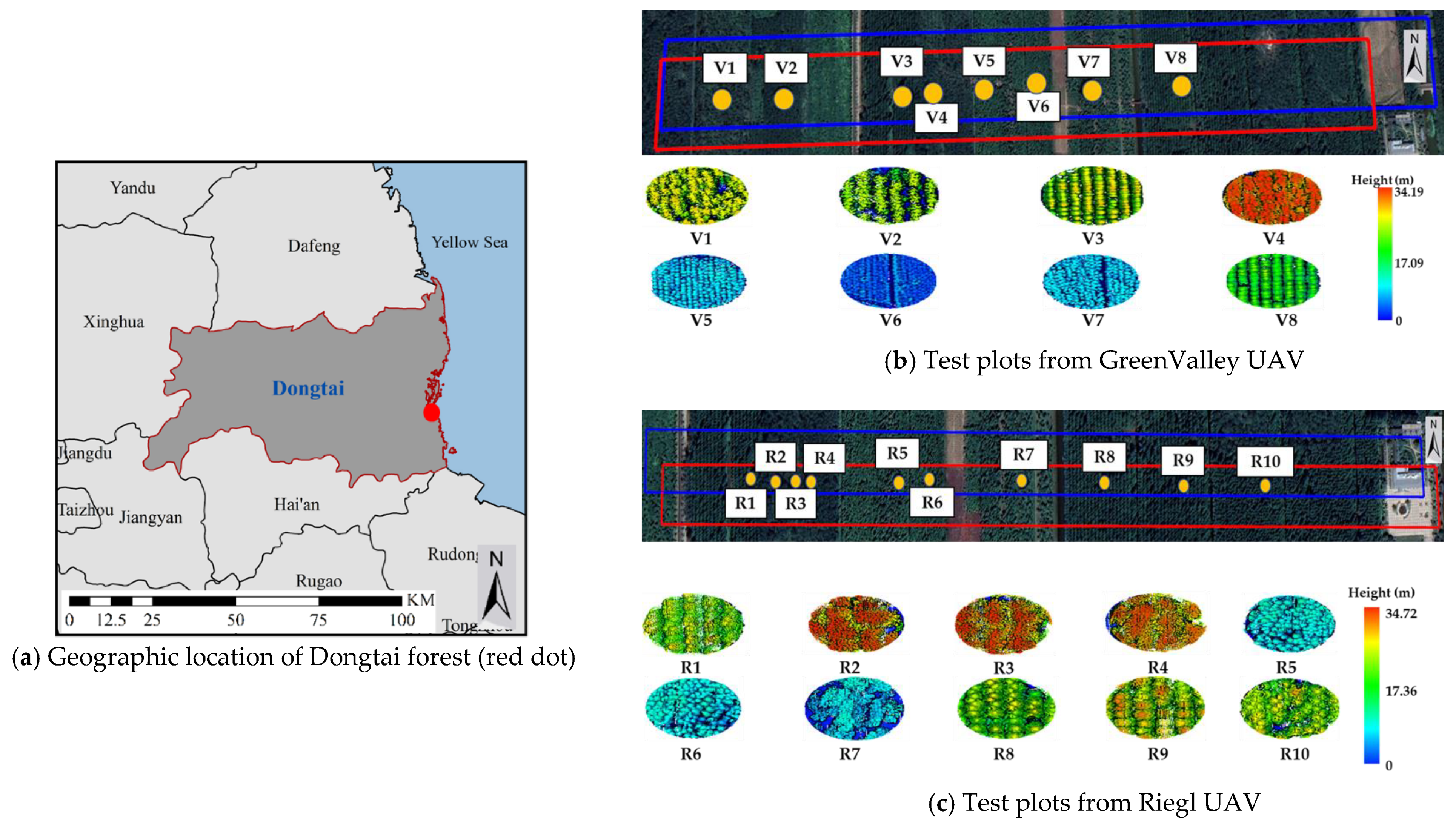
In a survey of the Velodyne UAV results considering the tree species, for plots V2 (deciduous), and plot V3 (conifer) with the same stem density, plot V3 has a higher matching percentage (82%) than plot V2 (55%), as well as demonstrating better matched point counts. Applying the same comparison between plots V3 and V5, plot V3 achieves much higher values because of the low tree heights of plot V5; however, both plots are conifer. This conclusion is supported by the results of plots V7 and V8, which have the same forest parameters, except that plot V8 has higher trees and, therefore, higher matching (63%).

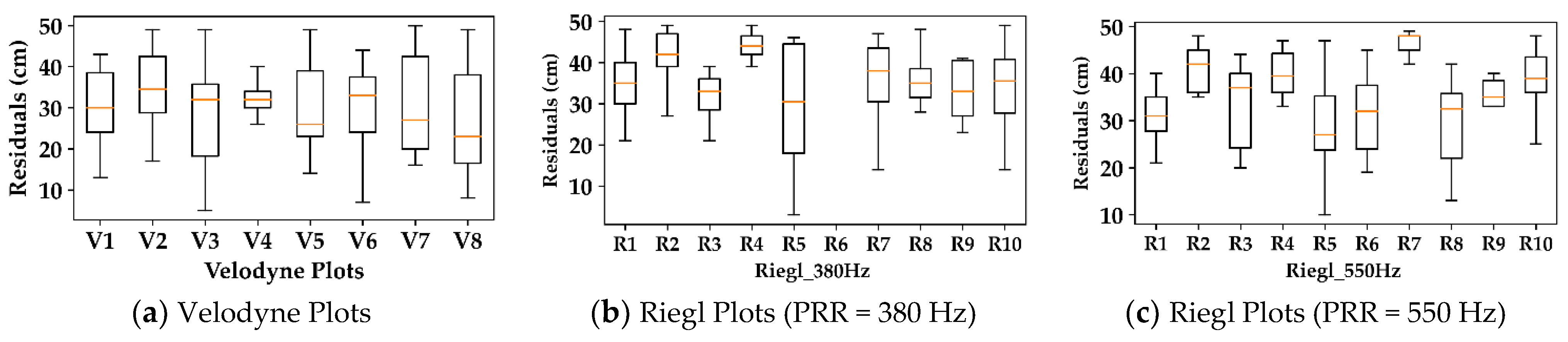
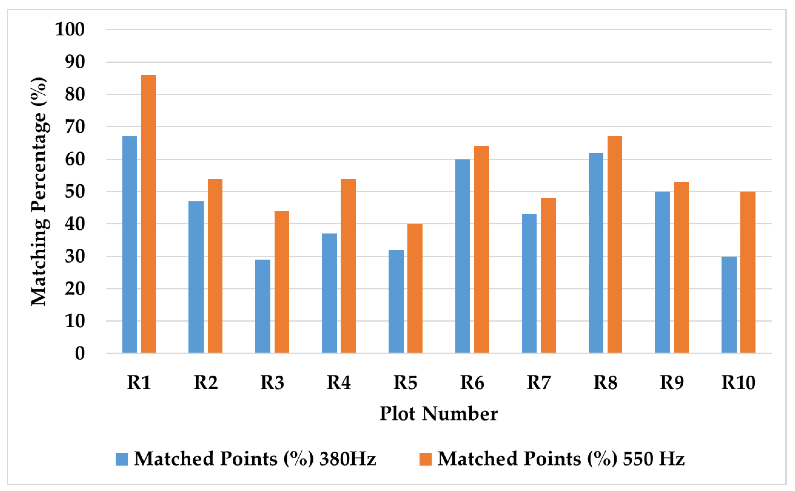
In the case of the Riegl dataset, the data are offered in two Pulse Repetition Frequencies (PRFs), enabling more analysis factors. The outcome of any tree parameter could be observed in both frequencies, as well as how much the frequency affects the results. In the context of laser waves, it is stated that the pulse energy equals the average transmitted power divided by the repetition rate, which means that the higher the PRR, the lower the pulse energy. Therefore, the PRR is a critical factor for any LiDAR sensor because it controls the point density, which is valuable for rich and detailed geoinformation extraction; however, lowering the pulse energy will result in accuracy degradation of the measured range. All the poplar plots from Riegl have the same stand density (208 tree/ha) and roughly the same tree height, except for R7, which had lower trees than the others. The matching percentages of these poplar plots at 550 Hz are consistently greater than their corresponding values at 380 Hz, as shown in Figure 12. This can be attributed to the high point density offered by the higher frequency data because the matching percentage increased in all cases, even for the lower trees in plot R7. However, the coniferous plots deliver different forest parameters for plots R6 and R8 with the same stem density and tree species (conifer), but R6 has lower tree heights, so R6 demonstrates a lower matching than R8 in both data frequencies. In Table 5, the mean of the 3D distance residuals at the matched points after alignment for both PRR frequencies has no significant difference, and 8 cm is the maximum difference that occurred for the coniferous plot R1, with the lowest stand density of the dawn redwood plots. This plot has relatively higher trees and a higher matching percentage over its conjugate from the 380 Hz dataset. Even though the matching percentages are consistently higher due to the point density, the resulting distance residuals at the matched points do not show a considerable improvement over those of the low frequency data, and in some cases are less accurate (e.g., test plots R6, R7, R9, and R10). The test plot R7 has a deciduous tree species with a low height of 8.6 m and stem density of 208 tree/ha. These parameters outweigh the accuracy reduction caused by the lower energy with an increasing range, along with the irregular crown shape of poplar trees. This is also supported by the results of R6 and R8 when considering the tree height difference of both, even though they have the same species (coniferous) and the same stem density. Moreover, the test plots R9 and R10 had the same stand density and relatively higher trees, and similar results were obtained for both PRFs. This implies that, although the high-frequency data have more dense points than the low-frequency data, the results are not necessarily high due to energy degradation.

From the dataset perspective and after referring to Table 1 and Table 2, which list the plot parameters, it is observed that the test plots V7 and R6 have the same parameters except tree height, which is not significantly different. Their matching percentages were 18% and 60% for V7 and R6, respectively. The lower tree heights (<8 m) are the cause for this large difference (42%) in matching percentage, which indicates that the higher point density in the case of the Riegl dataset reflects better matching percenatge, while the distance residuals vary within 5 cm and equal the residue for the 550 Hz data. Another case supporting this hypothesis is the relation between plots V8 and R8 with the same tree species (coniferous), stand density, and comparatively higher trees (~20 m). The matching of plot V8 equals 63%, whereas plot R8 matching percenatge is 62% and 67% for 380 Hz and 550 Hz data, respectively, without a significant variation in alignment accuracy (28 cm for V8 and 29 cm for R8), which also suggests that the higher trees have dense points due to the closeness to their scanning sensor, and consequently, the high-density point cloud has a higher matching percentage.

Furthermore, the poplar plots V4, R2, R3, and R4 have a stand density of 208 tree/ha and comparatively high trees. The matching percentage of plot V4 is 52%, whereas the plots R2, R3, and R4 have matching ranges from 29% to 47% and 44% to 54% for 380 Hz and 550 Hz data, respectively, with alignment accuracies of 31 cm for plot V4 and a maximum of 39 cm for other plots. The reduced stem density with the same tree heights with only changing the PRR (laser energy) or flight altitude (which is lower for Velodyne UAV) affect the matching percentage, and the Riegl higher frequency (550 Hz) compensates for the change in flight altitude.

Another evaluation criterion is the verification of the results on real data points (tree locations). First, tree segmentation is performed for both source and target point clouds before alignment and for the target point cloud after alignment. Then, the aligned trees are manually inspected.

Table 6. The percentage of matched trees after alignment from the Velodyne test plots.

Plot Id	Species	Percentage of Matched Trees < 0.50 m	Percentage of Matched Trees < 1 m
V1	Poplar	13	44
V2	Poplar	20	48
V3	Redwood	85	88
V4	Poplar	34	59
V5	Redwood	57	67
V6	Redwood	26	50
V7	Redwood	43	53
V8	Redwood	68	78

shows the results of this experiment on Velodyne LiDAR test plots.

The results are promising for both poplar and redwood forest plots. The lowest percentage of matched trees for the poplar plots is 44% and the corresponding value for the conifer plots is 50%. The percentage of matched trees for poplar plots ranges from 44% to 59% at 1m distance while the corresponding range for conifer trees plots is from 50% to 88% at the same distance threshold. Then the method achieves reliable results when evaluated with trees locations.

Comparison with Baseline

The results were compared with the baseline method [8] which performed the ALS and terrestrial photogrammetric point cloud co-registration using features from the planimetric and vertical distances between the trees’ locations within the same forest plot. They separated the process into two stages: 2D rigid transformation (one rotation and two translations) and a vertical offset correction. The optimal 2D transformation parameters are obtained by a heuristic search over the correspondences set starting from an initial solution. This method is applied here to the tree locations of the eight plots provided from a point cloud segmentation on LiDAR360 software [45] which segments the air-based point cloud data depending on the global maximum and the gap between neighboring trees [46]. The comparison is performed in 2D space on the planimetric deviations at the matched points before and after alignment.

Table 7. Summary of comparison results between the proposed method and baseline method.

Plot Id	Tree Species	Matching Percentage (%)		Mean Planimetric Distance Residuals (cm)
		Object-Based	Our Method	Object-Based	Our Method
V1	Poplar	35	43	30	27
V2		52	55	31	32
V4		48	52	34	28
V3	Dawn redwood	60	82	37	23
V5		11	39	27	25
V6		16	29	27	28
V7		37	18	36	23
V8		48	63	28	17

, in which the baseline method is called “object-based,” lists the comparison results in two groups: for the poplar plots, the matching percentage is increased by 3% to 8% for plots V2 and V1, respectively. The average deviation after alignment was 3–6 cm except for plot V2, which has no significant difference in the planimetric distance residual. In contrast, the conifer plots incorporate various parameters, thereby affecting the accuracy of matching and alignment.

The test plots V3 and V8 resulted in a higher matching percentage than the baseline; however, V8 has a stem density more than triple that of plot V3, and the distance residuals for both plots were clearly enhanced above 10 cm compared with the baseline method. The key factor here is tree height, as both plots have higher trees. This can be validated by the case of plots V3 and V6; however, they have equal stem density. The change in tree heights affects the tree localization accuracy as the matching percentage of the baseline method is 16%, and it is increased to 29% using our method because the intended method does not depend on tree segmentation. The baseline method achieved a better match at plot V7, but the mean of distance residuals at matched points is improved by 13 cm in our method, which can be clarified by the extremely high stand density of the plot, which accordingly affects tree localization and tree height.

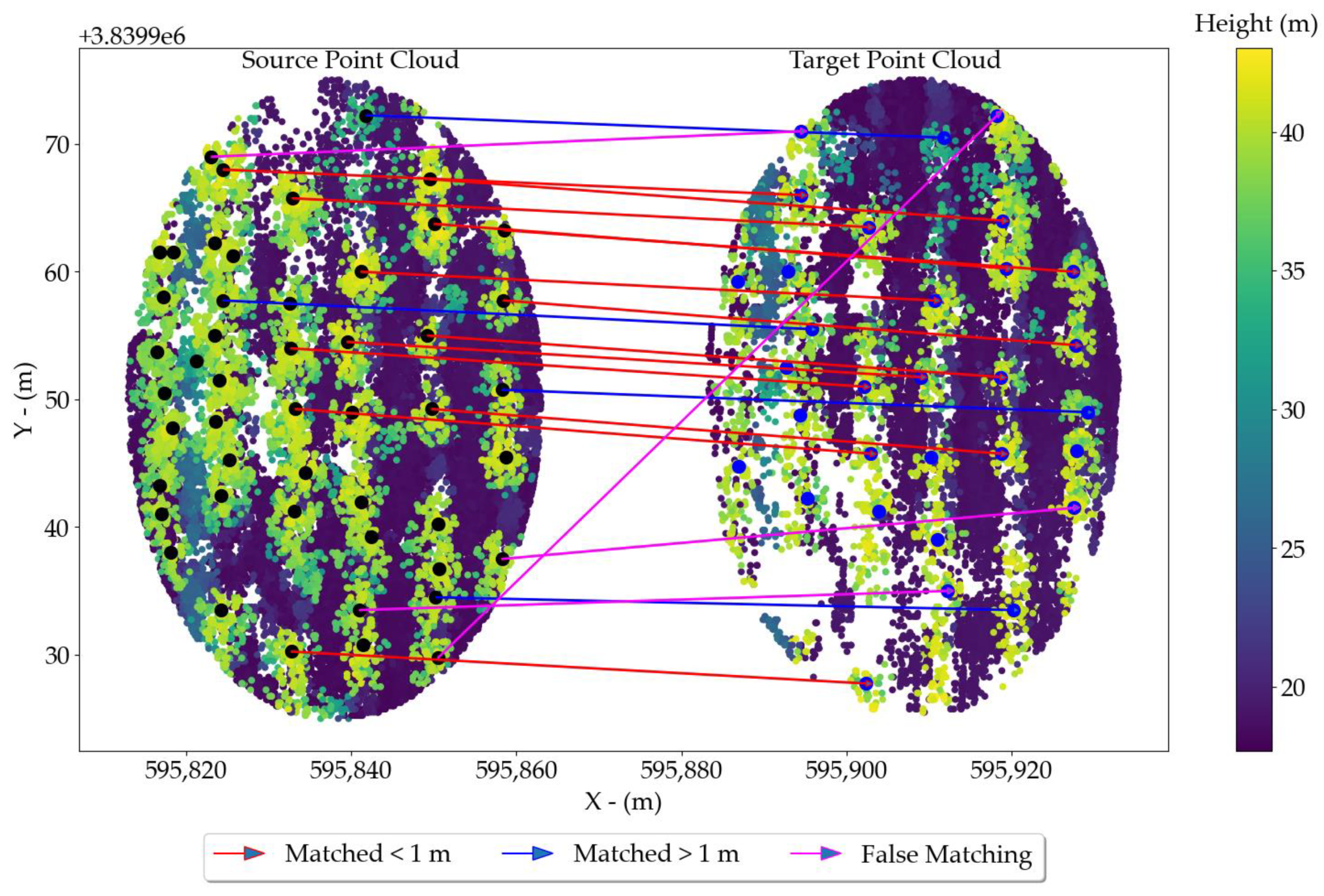
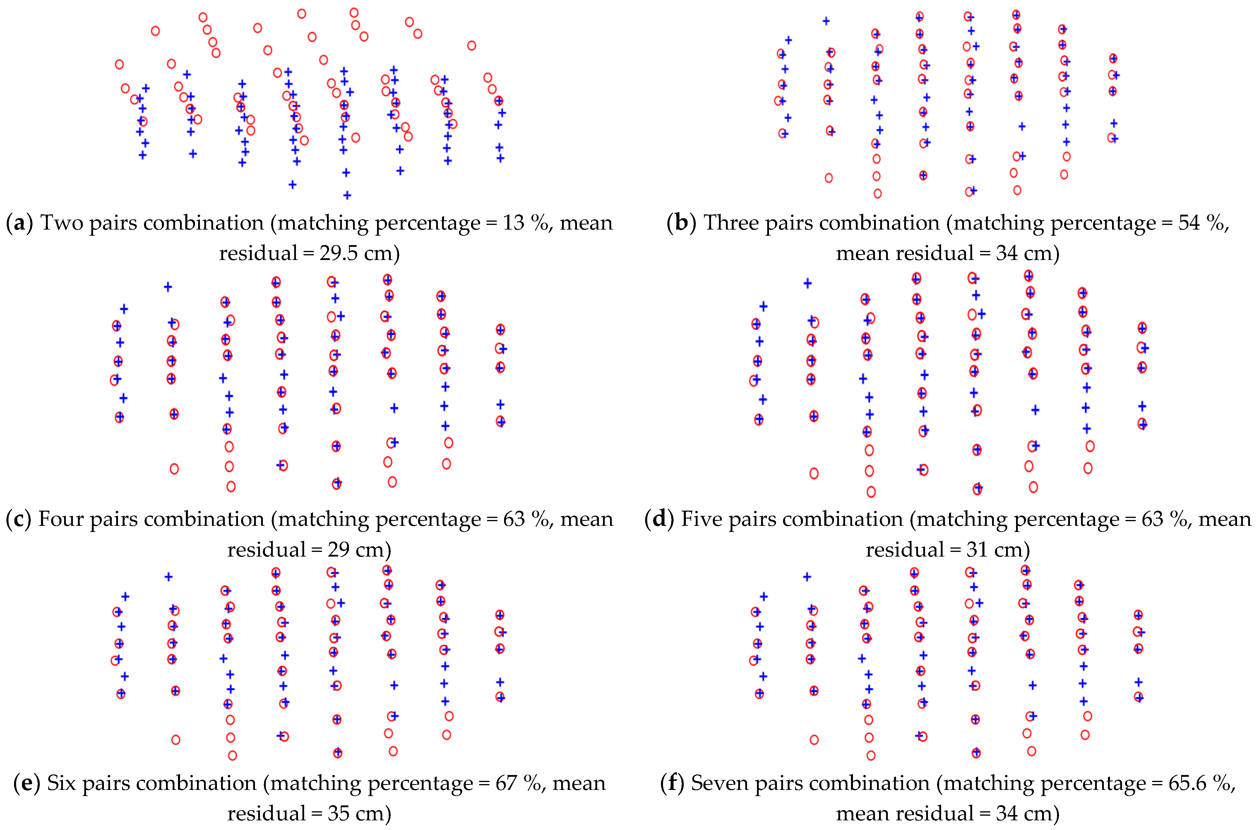
The results presented for all plots show that there are still differences between the keypoints after alignment, as shown in Figure 8b–f). These differences reflect the performance of the proposed alignment method. The reasons for these differences include the accuracy of keypoint extraction, the matching algorithm, and the optimization of the transformation function. Strip alignment with the introduced method may not have a good performance with low-density or extremely low tree heights, where it is challenging to distinguish the canopy. The method needs to be tested against a dataset from an actual forest stand despite the large number of experiments from the planted forest introduced in this work.

6. Conclusions and Outlook

This work introduced a fully automated method for UAV strip alignment in forested areas, necessitating only the existence of the canopy cover, which is the hallmark of the LiDAR data collected by air-based platforms. Moreover, a density-based canopy clustering is performed using the HDBSCAN algorithm, which requires only one input parameter and discovers the clusters of arbitrary shapes without the need to predict the number of clusters. The main advantage of the proposed method is the ability to overcome the limitations of tree localization when working on complex forests (deciduous tree species, high stem density, and high near-ground vegetation) or windy environments. Additionally, the method performs the 3D transformation of the overlapping strips without any extra information regarding the tree parameters (e.g., tree height and DBH) or altitudes from a digital elevation model of the area using the virtual keypoints. The method was tested on eighteen circular test plots comprising poplar and dawn redwood tree species with two case studies: eight plots (50 m in diameter) cropped from Velodyne VLP-16 UAV data, whereas the remaining pairs (30 m in diameter) were picked from Riegl VUX-1 data offered in two PRFs (380 Hz and 550 Hz). The Euclidean distance discrepancies were compared before and after alignment at the matched points to evaluate the alignment results. The range of 3D deviations after alignment for the poplar plots was from 31 cm to 36 cm, whereas the same range of dawn redwood plots was from 28 cm to 31 cm in the case of Velodyne UAV plots. For the two PRFs offered by the Riegl UAV, the 3D discrepancies at the matched points after alignment were not significantly different, with the mean values at the dawn redwood plots of 33 cm and 32 cm for the 380 Hz and 550 Hz data, respectively, whereas their corresponding values were 38 cm and 39 cm for the poplar plots. The high-frequency data (550 Hz) consistently produce a higher matching percentage than the low-frequency (380 Hz) plots because of the high point density, while the 3D distance residuals after alignment are not considerably different for both frequencies. The performance of the proposed method would be poor for extremely low tree heights and/or for data with very low canopy point density, since it is mainly based on canopy clustering. Also, experiments were limited to planted forest plots where flat topography, regular forest structure, and approximately equal tree parameters are present at the plot level. However, the strip alignment of point clouds from forest plantations is more challenging than for natural forests due to the characteristics of the planted forest, which makes feature matching more complicated. Therefore, the strip alignment of point clouds from natural forests would be challenging to the proposed method due to their rough terrain, but this can be handled by height normalization using a DEM created from the point cloud itself. The diversity of tree species, shapes, and parameters in natural forest plots, which in turn provide more irregular crown shapes need to be explored by the proposed method. It would be interesting to use the proposed method in estimating more representative forest parameters, such as canopy volume and tree height, especially in the case of air-based platform co-registration or with more parameters (e.g., DBH and stem curve) in the case of multi-platform point cloud data integration.

References

1. Zealand, N. The Role of Planted Forests in Sustainable Forest Management; Governments of Chile, Denmark, India, New Zealand and Portugal: Santiago, Chile, 1999. [Google Scholar]
2. Wieser, M.; Hollaus, M.; Mandlburger, G.; Glira, P.; Pfeifer, N. ULS LiDAR Supported Analyses of Laser Beam Penetration from Different ALS Systems into Vegetation. In Proceedings of the ISPRS Annals of Photogrammetry, Remote Sensing and Spatial Information Sciences, Prague, Czech Republic, 12–19 July 2016; Volume III–3, pp. 233–239. [Google Scholar]
3. Rönnholm, P.; Liang, X.; Kukko, A.; Jaakkola, A.; Hyyppä, J. Quality Analysis and Correction of Mobile Backpack Laser Scanning Data. In Proceedings of the ISPRS Annals of the Photogrammetry, Remote Sensing and Spatial Information Sciences, Prague, Czech Republic, 12–19 July 2016; Volume 3, pp. 41–47. [Google Scholar]
4. Guimarães, N.; Pádua, L.; Marques, P.; Silva, N.; Peres, E.; Sousa, J.J. Forestry remote sensing from unmanned aerial vehicles: A review focusing on the data, processing and potentialities. Remote Sens. 2020, 12, 1046. [Google Scholar] [CrossRef] [Green Version]
5. Brede, B.; Lau, A.; Bartholomeus, H.M.; Kooistra, L. Comparing RIEGL RiCOPTER UAV LiDAR derived canopy height and DBH with terrestrial LiDAR. Sensors 2017, 17, 2371. [Google Scholar] [CrossRef] [PubMed]
6. Liu, K.; Shen, X.; Cao, L.; Wang, G.; Cao, F. Estimating forest structural attributes using UAV-LiDAR data in Ginkgo plantations. ISPRS J. Photogramm. Remote Sens. 2018, 146, 465–482. [Google Scholar] [CrossRef]
7. Guo, Q.; Su, Y.; Hu, T.; Zhao, X.; Wu, F.; Li, Y.; Liu, J.; Chen, L.; Xu, G.; Lin, G.; et al. An integrated UAV-borne lidar system for 3D habitat mapping in three forest ecosystems across China. Int. J. Remote Sens. 2017, 38, 2954–2972. [Google Scholar] [CrossRef]
8. Corte, A.P.D.; Souza, D.V.; Rex, F.E.; Sanquetta, C.R.; Mohan, M.; Silva, C.A.; Zambrano, A.M.A.; Prata, G.; Alves de Almeida, D.R.; Trautenmüller, J.W.; et al. Forest inventory with high-density UAV-Lidar: Machine learning approaches for predicting individual tree attributes. Comput. Electron. Agric. 2020, 179, 105815. [Google Scholar] [CrossRef]
9. Magri, F.; Orcid, T. A Lightweight UAV-Based Laser Scanning System For Forest Application. Bull. Geod. Sci. 2018, 24, 318–334. [Google Scholar]
10. Morsdorf, F.; Eck, C.; Zgraggen, C.; Imbach, B.; Schneider, F.D.; Kükenbrink, D. UAV-based LiDAR acquisition for the derivation of high-resolution forest and ground information. Lead. Edge 2017, 36, 566–570. [Google Scholar] [CrossRef]
11. Ferraz, A.; Bretar, F.; Jacquemoud, S.; Gonçalves, G.; Pereira, L.; Tomé, M.; Soares, P. 3-D mapping of a multi-layered Mediterranean forest using ALS data. Remote Sens. Environ. 2012, 121, 210–223. [Google Scholar] [CrossRef]
12. Eysn, L.; Hollaus, M.; Lindberg, E.; Berger, F.; Monnet, J.-M.; Dalponte, M.; Kobal, M.; Pellegrini, M.; Lingua, E.; Mongus, D.; et al. A Benchmark of Lidar-Based Single Tree Detection Methods Using Heterogeneous Forest Data from the Alpine Space. Forests 2015, 6, 1721–1747. [Google Scholar] [CrossRef] [Green Version]
13. Dong, T.; Zhou, Q.; Gao, S.; Shen, Y. Automatic Detection of Single Trees in Airborne Laser Scanning Data through Gradient Orientation Clustering. Forests 2018, 9, 291. [Google Scholar] [CrossRef] [Green Version]
14. Yun, T.; Jiang, K.; Li, G.; Eichhorn, M.P.; Fan, J.; Liu, F.; Chen, B.; An, F.; Cao, L. Individual tree crown segmentation from airborne LiDAR data using a novel Gaussian filter and energy function minimization-based approach. Remote Sens. Environ. 2021, 256, 112307. [Google Scholar] [CrossRef]
15. Brovkina, O.; Cienciala, E.; Surový, P.; Janata, P. Unmanned aerial vehicles (UAV) for assessment of qualitative classification of Norway spruce in temperate forest stands. Geo-Spatial Inf. Sci. 2018, 21, 12–20. [Google Scholar] [CrossRef] [Green Version]
16. Filin, S. Recovery of Systematic Biases in Laser Altimetry Data Using Natural Surfaces. Photogramm. Eng. Remote Sens. 2013, 69, 1235–1242. [Google Scholar] [CrossRef]
17. Habib, A.F.; Kersting, A.P.; Ruifang, Z.; Al-Durgham, M.; Kim, C.; Lee, D.C. Lidar strip adjustment using conjugate linear features in overlapping strips. In Proceedings of the The International Archives of the Photogrammetry, Remote Sensing and Spatial Information Siences, Beijing, China, 3–11 July 2008; Volume 37, pp. 385–390. [Google Scholar]
18. Polewski, P.; Erickson, A.; Yao, W.; Coops, N.; Krzystek, P.; Stilla, U. Object-Based Coregistration of Terrestrial Photogrammetric and ALS Point Clouds in Forested Areas. In Proceedings of the ISPRS Annals of the Photogrammetry, Remote Sensing and Spatial Information Sciences, Prague, Czech Republic, 12–19 July 2016; Volume 3, pp. 347–354. [Google Scholar]
19. Dai, W.; Yang, B.; Liang, X.; Dong, Z.; Huang, R.; Wang, Y.; Pyörälä, J.; Kukko, A. Fast registration of forest terrestrial laser scans using key points detected from crowns and stems. Int. J. Digit. Earth 2020, 13, 1–19. [Google Scholar] [CrossRef]
20. Dai, W.; Yang, B.; Liang, X.; Dong, Z.; Huang, R.; Wang, Y.; Li, W. Automated fusion of forest airborne and terrestrial point clouds through canopy density analysis. ISPRS J. Photogramm. Remote Sens. 2019, 156, 94–107. [Google Scholar] [CrossRef]
21. Kelbe, D.; Van Aardt, J.; Romanczyk, P.; Van Leeuwen, M.; Cawse-Nicholson, K. Multiview Marker-Free Registration of Forest Terrestrial Laser Scanner Data with Embedded Confidence Metrics. IEEE Trans. Geosci. Remote Sens. 2017, 55, 729–741. [Google Scholar] [CrossRef]
22. Paris, C.; Kelbe, D.; Van Aardt, J.; Bruzzone, L. A Novel Automatic Method for the Fusion of ALS and TLS LiDAR Data for Robust Assessment of Tree Crown Structure. IEEE Trans. Geosci. Remote Sens. 2017, 55, 3679–3693. [Google Scholar] [CrossRef]
23. Shao, J.; Zhang, W.; Mellado, N.; Wang, N.; Jin, S.; Cai, S.; Luo, L.; Lejemble, T.; Yan, G. SLAM-aided forest plot mapping combining terrestrial and mobile laser scanning. ISPRS J. Photogramm. Remote Sens. 2020, 163, 214–230. [Google Scholar] [CrossRef]
24. Li, Q.; Nevalainen, P.; Queralta, J.P.; Heikkonen, J.; Westerlund, T. Localization in unstructured environments: Towards autonomous robots in forests with Delaunay triangulation. Remote Sens. 2020, 12, 1870. [Google Scholar] [CrossRef]
25. Fekry, R.; Yao, W.; Cao, L. Automated UAV-Lidar Strip Alignment in Forested Areas Using Density Based Canopy Clustering. In Proceedings of the ISPRS Annals of Photogrammetry, Remote Sensing and Spatial Information Sciences, Nice, France, 31 August–2 September 2020; Volume V-1–2020, pp. 81–88. [Google Scholar]
26. Persad, R.A.; Armenakis, C. Automatic co-registration of 3D multi-sensor point clouds. ISPRS J. Photogramm. Remote Sens. 2017, 130, 162–186. [Google Scholar] [CrossRef]
27. Glira, P.; Pfeifer, N.; Briese, C.; Ressl, C. A Correspondence Framework for ALS Strip Adjustments based on Variants of the ICP Algorithm Korrespondenzen für die ALS-Streifenausgleichung auf Basis von ICP. Photogramm. Fernerkundung Geoinf. 2015, 2015, 275–289. [Google Scholar] [CrossRef]
28. Glira, P.; Pfeifer, N.; Briese, C.; Ressl, C. Rigorous strip adjustment of airborne laserscanning data based on the icp algorithm. ISPRS Ann. Photogramm. Remote Sens. Spat. Inf. Sci. 2015, 2, 73–80. [Google Scholar] [CrossRef] [Green Version]
29. Zhang, Y.; Xiong, X.; Zheng, M.; Huang, X. LiDAR Strip Adjustment Using Multifeatures Matched With Aerial Images. IEEE Trans. Geosci. Remote Sens. 2015, 53, 976–987. [Google Scholar] [CrossRef]
30. Polewski, P.; Yao, W. Scale invariant line-based co-registration of multimodal aerial data using L1 minimization of spatial and angular deviations. ISPRS J. Photogramm. Remote Sens. 2019, 152, 79–93. [Google Scholar] [CrossRef]
31. Lee, J.; Yu, K.; Kim, Y.; Habib, A.F. Adjustment of discrepancies between LIDAR data strips using linear features. IEEE Geosci. Remote Sens. Lett. 2007, 4, 475–479. [Google Scholar] [CrossRef]
32. Prokop, M.; Shaikh, S.A.; Kim, K.-S.S. Low Overlapping Point Cloud Registration Using Line Features Detection. Remote Sens. 2020, 12, 61. [Google Scholar] [CrossRef] [Green Version]
33. Teo, T.-A.; Huang, S.-H. Surface-Based Registration of Airborne and Terrestrial Mobile LiDAR Point Clouds. Remote Sens. 2014, 6, 12686–12707. [Google Scholar] [CrossRef] [Green Version]
34. Al-Rawabdeh, A.; He, F.; Habib, A. Automated Feature-Based Down-Sampling Approaches for Fine Registration of Irregular Point Clouds. Remote Sens. 2020, 12, 1224. [Google Scholar] [CrossRef] [Green Version]
35. Xu, Y.; Boerner, R.; Yao, W.; Hoegner, L.; Stilla, U. Pairwise coarse registration of point clouds in urban scenes using voxel-based 4-planes congruent sets. ISPRS J. Photogramm. Remote Sens. 2019, 151, 106–123. [Google Scholar] [CrossRef]
36. Polewski, P.; Yao, W.; Cao, L.; Gao, S. Marker-free coregistration of UAV and backpack LiDAR point clouds in forested areas. ISPRS J. Photogramm. Remote Sens. 2019, 147, 307–318. [Google Scholar] [CrossRef]
37. Guan, H.; Su, Y.; Hu, T.; Wang, R.; Ma, Q.; Yang, Q.; Sun, X.; Li, Y. A Novel Framework to Automatically Fuse Multiplatform LiDAR Data in Forest Environments Based on Tree Locations. IEEE Trans. Geosci. Remote Sens. 2019, 58, 1–13. [Google Scholar] [CrossRef]
38. Riegel VUX1-UAV. Available online: http://www.riegl.com/products/unmanned-scanning/riegl-vux-1uav/ (accessed on 8 May 2019).
39. Nobuyuki Otsu A Threshold Selection Method from Gray-Level Histograms. IEEE Trans. Syst. Man Cybern 1979, 9, 62–66. [CrossRef] [Green Version]
40. Campello, R.J.G.B.; Moulavi, D.; Sander, J. Density-based clustering based on hierarchical density estimates. In Proceedings of the Advances in Knowledge Discovery and Data Mining, Gold Coast, Australia, 14–17 April 2013; Volume 7819, pp. 160–172. [Google Scholar]
41. Ester, M.; Kriegel, H.-P.; Sander, J.; Xu, X. A Density-Based Algorithm for Discovering Clusters in Large Spatial Databases with Noise. In Proceedings of the 2nd International Conference on Knowledge Discovery and Data Mining, Menlo Park, CA, USA, 31 December 1996; Volume 2, pp. 226–231. [Google Scholar]
42. Ying, Z.; Gu, S.; Tomasi, C. Topological Persistence On A Jordan Curve. In Proceedings of the International Conference on Acoustics, Speech, and Signal Processing (ICASSP), Kyoto, Japan, 25–30 March 2012; pp. 3693–3696. [Google Scholar]
43. Zhou, D.; Li, G.; Liu, Y.H. Effective corner matching based on delaunay triangulation. In Proceedings of the IEEE International Conference on Robotics and Automation, New Orleans, LA, USA, 26 April–1 May 2004; pp. 2730–2735. [Google Scholar]
44. Edmonds, J.; Richard, M.K. Theoretical Improvements in Algorithmic Efficiency for Network Flow Problems. J. ACM 1972, 19, 248–264. [Google Scholar] [CrossRef]
45. LiDAR360. Available online: https://greenvalleyintl.com/software/lidar360/ (accessed on 18 November 2020).
46. Li, W.; Guo, Q.; Jakubowski, M.K.; Kelly, M. A New Method for Segmenting Individual Trees from the Lidar Point Cloud. Photogramm. Eng. Remote Sens. 2012, 78, 75–84. [Google Scholar] [CrossRef] [Green Version]
Figure 1. Visualization of discrepancies between overlapping UAV-LiDAR strips. (top row: a pair of overlapping strips, middle row: a profile within the overlap area in two perpendicular direction before alignment, and bottom row: the alignment.).
Ijgi 10 00284 g001
Figure 2. Presentation of study area. (a) Geographic location of Dongtai forest. (b) Strip pair from GreenValley UAV (Velodyne dataset, overlap ≥ 80 %). (c) Strip pair from Riegl UAV (Riegl dataset, overlap ≥ 45 %). The red and blue rectangles in (a) and (b) represent the south strip and the north strip, respectively. The color bars in (b) and (c) indicate the height above ground level to show the tree heights.
Ijgi 10 00284 g002
Figure 3. Research workflow.
Ijgi 10 00284 g003
Figure 4. Visualization of height histogram analysis in two cases. (a) poplar plot, (b) coniferous plot. Blue lines indicate the detected dividing heights.
Ijgi 10 00284 g004
Figure 5. Overview of keypoint extraction for a single cluster using topological persistence.
Ijgi 10 00284 g005
Figure 6. Canopy clustering and keypoint extraction: samples from poplar tree species (top row (a,b)) and dawn redwood plot (bottom row (c,d)), with the color gradient indicating the height. The left column shows the raw point cloud data, different colors in the right column represent the individual clusters, and the black dots are the extracted keypoints.
Ijgi 10 00284 g006
Figure 7. One-to-one correspondence from graph matching.
Ijgi 10 00284 g007
Figure 8. Alignment results of keypoints by permutation over the correspondences set. Best transformation comes from four pair combination with the lowest mean distance residuals.
Ijgi 10 00284 g008
Figure 9. The distance residuals after alignment at the matched points for all test plots. The orange lines represent the median of the residual values of the matched at individual plots.
Ijgi 10 00284 g009
Figure 10. Sample of the alignment results of Velodyne plots (top row: profile from dawn redwood plot, bottom row: profile from poplar plot). The red color represents the point cloud data from the south strip while the green color dataset belongs to the north strip.
Ijgi 10 00284 g010aIjgi 10 00284 g010b
Figure 11. Profile from the alignment results of a coniferous test plot by Riegl UAV at two PRFs (top row: 380 Hz, bottom row: 550 Hz). The green and red colors represent the point cloud of north and south strips, respectively.
Ijgi 10 00284 g011
Figure 12. Summary of matching results of all Riegl plots at the two PRFs.
Ijgi 10 00284 g012