Maximizing Impacts of Remote Sensing Surveys in Slope Stability—A Novel Method to Incorporate Discontinuities into Machine Learning Landslide Prediction

Abstract

This paper proposes a novel method to incorporate unfavorable orientations of discontinuities into machine learning (ML) landslide prediction by using GIS-based kinematic analysis. Discontinuities, detected from photogrammetric and aerial LiDAR surveys, were included in the assessment of potential rock slope instability through GIS-based kinematic analysis. Results from the kinematic analysis, coupled with several commonly used landslide influencing factors, were adopted as input variables in ML models to predict landslides. In this paper, various ML models, such as random forest (RF), support vector machine (SVM), multilayer perceptron (MLP) and deep learning neural network (DLNN) models were evaluated. Results of two validation methods (confusion matrix and ROC curve) show that the involvement of discontinuity-related variables significantly improved the landslide predictive capability of these four models. Their addition demonstrated a minimum of 6% and 4% increase in the overall prediction accuracy and the area under curve (AUC), respectively. In addition, frequency ratio (FR) analysis showed good consistency between landslide probability that was characterized by FR values and discontinuity-related variables, indicating a high correlation. Both results of model validation and FR analysis highlight that inclusion of discontinuities into ML models can improve landslide prediction accuracy.

1. Introduction

Landslides have drawn world-wide attention due to their potentially devastating impact on human safety and infrastructure. It has been reported that the total land area over the world subjected to landslides is about 3.7 million square kilometers, affecting a population of nearly 300 million [1]. In addition, the relatively high-risk areas (top three deciles) cover about 820,000 square kilometers with an estimated population of 66 million. In recent decades, examples of catastrophic landslide events have been recorded in different regions globally. In 2011, multiple rapid deep-seated landslides resulted in the obstruction of river valleys by landslide-formed dams, being in danger of dam breach, upstream inundation, and downstream flooding [2]. In 2014, the Gold Basin landslide occurred in the USA, damaging 49 houses down the slope and causing 43 fatalities [3]. A catastrophic high-elevation and long-runout landslide occurred in China, causing the death of 51 people and the destruction and burial of 21 houses in 2019 [4].

Commonly, landslide analysis is carried out to evaluate the stability of a specific slope by exploring the potential failure mechanism and risk associated with a collapse. Following this, remedial measures can be employed to strengthen or provide reinforcement to the unstable slope [5]. With the development of computer science, state-of-the-art machine learning methods have been established that mathematically simulate the relationships between landslides and their influencing factors. Among these statistical methods, conventional machine learning (ML) algorithms have been intensively used during recent years. For example, support vector machine (SVM) [6,7,8], decision tree analysis [9], random forest [9,10], and logistic regression [11,12] have been adopted to produce landslide susceptibility maps with high prediction accuracies. Recent developments in deep learning algorithms have also provided a basis for landslide analysis [13,14,15] that offer better performance and higher accuracy on landslide prediction to conventional ML algorithms.

Encouraging results from these papers indicate that ML methods can provide accurate landslide predictions, and have highlighted specific influencing factors of landslides developed in natural slopes (soil and rock). These factors are normally associated with geometric conditions (e.g., aspect, curvature, slope, cliff height) [8,16], geological conditions (e.g., lithology, faults) [11,17], hydrogeological conditions (e.g., rainfall, drainage) [9,16], topographic conditions (e.g., land cover/land use, vegetation) [13,18,19], etc. However, local discontinuities (such as joints, fractures and bedding planes), especially their orientations, have rarely been considered in ML landslide analyses even though many publications have highlighted that unfavorable orientations of discontinuities may cause rock slope failures [20,21,22,23,24]. Other studies have also emphasized that rock landslides are sensitive to changes in discontinuity properties. For example, Vatanpour et al. [25] used limit equilibrium analysis to demonstrate the importance of dip angle of discontinuity planes on slope stability. Havaej et al. [26] adopted a 3D brittle fracture approach emphasized the role of brittle fracture in the failure of the Vajont Slide. Vanneshi et al. [27], using a distinct element method, highlighted the importance of discontinuity orientations on potential toppling failure. In addition, conventional slope stability analysis methods, such as kinematic analysis and limit equilibrium, are based on inclusion of properties of discontinuities (orientation, strength, and roughness, etc.), highlighting their importance.

In this context, a novel application of unfavorably orientated discontinuities into ML landslide prediction is proposed by using GIS-derived kinematic analysis. Discontinuities, detected from remote sensing surveys obtained in areas prone to rock slope instability, were incorporated into GIS-based kinematic analysis. Results from the kinematic analysis were taken as additional input variables to improve the accuracy of ML landslide prediction algorithms. In addition, FR analysis was implemented to quantitatively investigate the potential relationship between the discontinuity-related variables and landslide occurrence.

The following paper highlights the benefit of point clouds in the extraction of geological discontinuities, through which GIS-based kinematic analysis is performed to assess the potential of rock slope failures, while also providing a novel application of the discontinuities to improve the accuracy of ML-based landslide prediction.

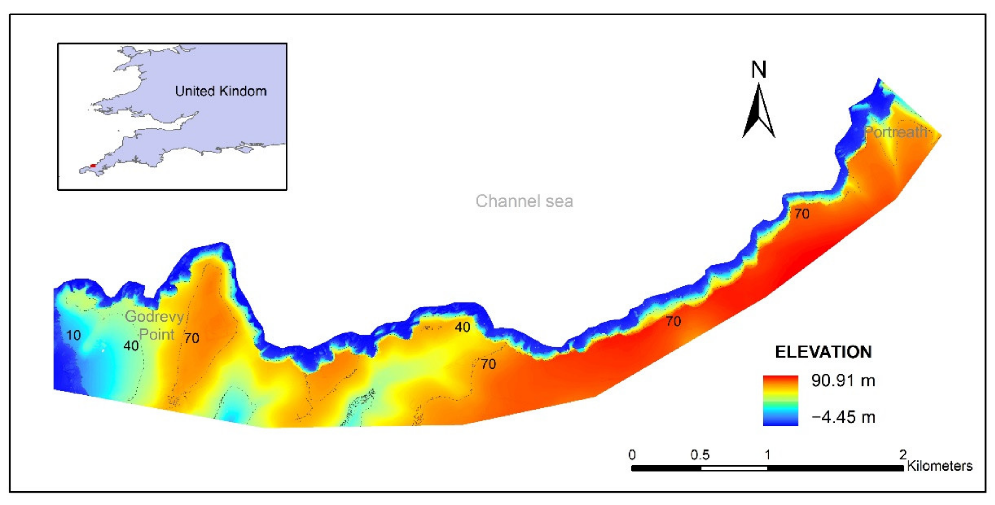
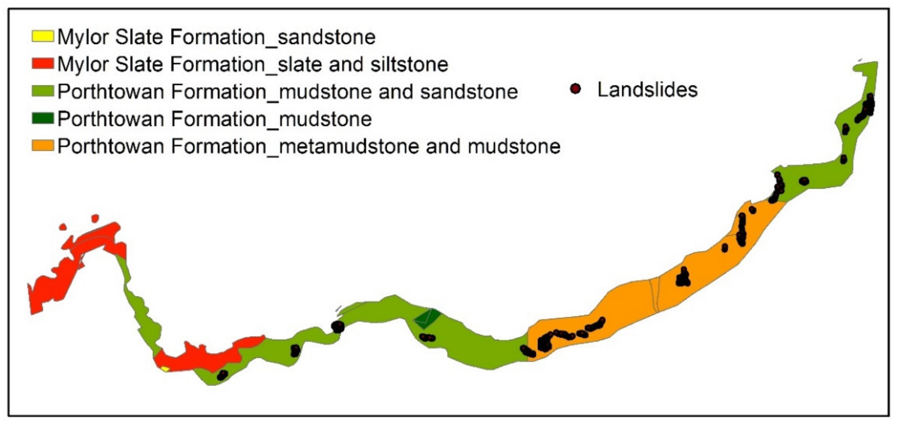
2. Study Area Description

This research study is focused on the North Coast of Cornwall, UK. The study area is a section of coastal rock cliff with a minimum height of 40 m between the Godrevy Point and Portreath (Figure 1), experiencing a warm temperate climate with an average yearly temperature of 10 °C and an average annual rainfall of 1062 mm. Almost half the annual rainfall occurs between October and January (approximately 500 mm), with a marked minimum from April to July. This section of steep coast is known to be prone to landslides of various sizes [28], with geological structures (such as faults and joints) playing a vital role in their occurrence [22].

The geology of the study area is dominated by the Porthtowan Formation (Gramscatho Group) [29], which comprises alternating beds of strong to moderately strong, medium to thinly bedded dark grey mudstone, interbedded with strong to moderately strong, thick to thinly bedded pale grey fine sandstone, which may locally have a silt and mud component [22,30].

3. Data and Methods

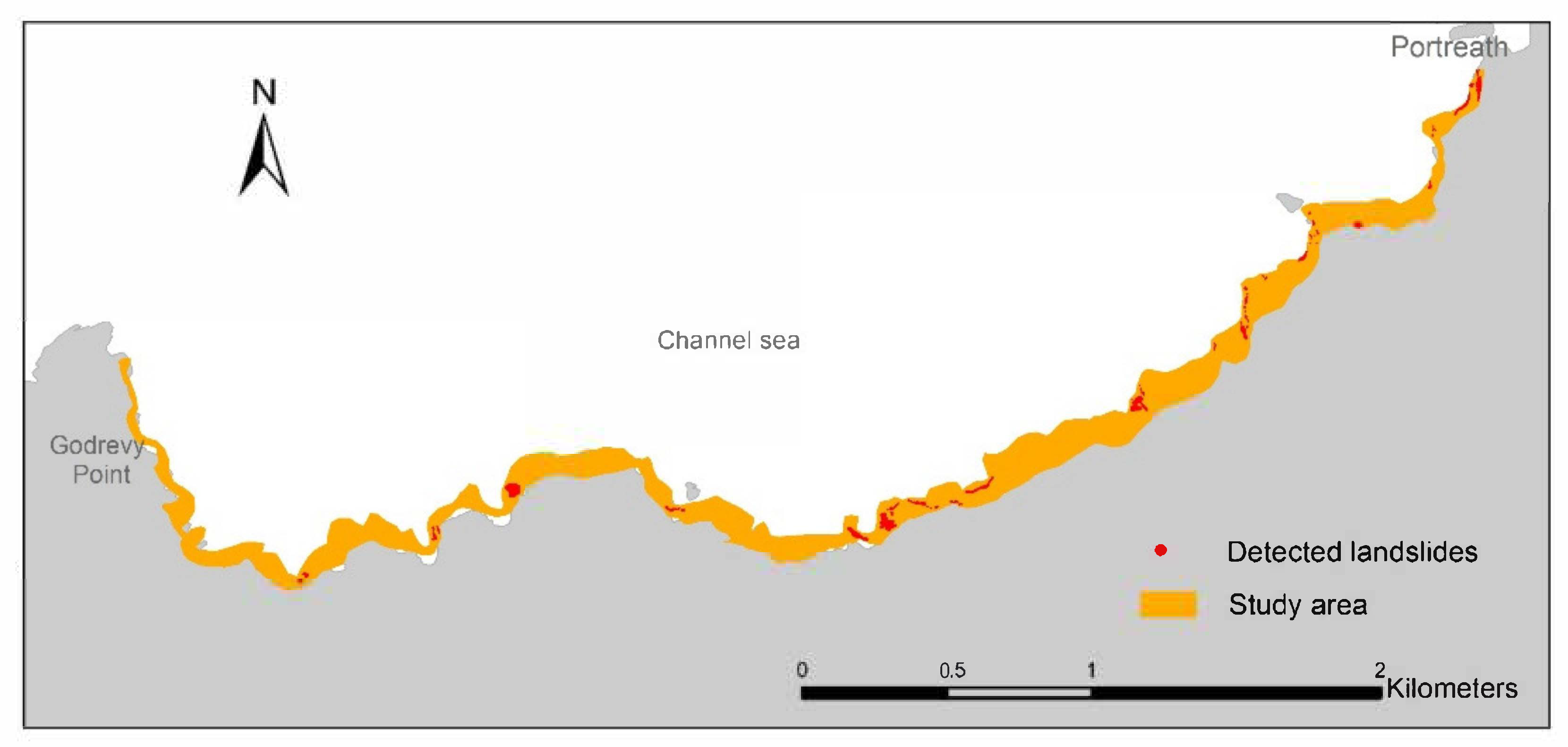
3.1. Landslide Detection and Sampling Strategy

Landslides were detected through a widely used method based on elevation change during a given time period [31,32,33]. It was implemented through a comparison of multitemporal LiDAR DEM data with 1 mpixel resolution and ±40 cm positional accuracy (years 2008 and 2014) collected from an open-source database (Digimap) [34]. Pixels with more than 5 m decreases in elevation from years 2008 to 2014 were recognized as potential landslides, with which the detection accuracy of landslides developed in the coastal cliff and the disturbance of noise points from LiDAR data, to some extent, could be balanced. Since ground truthing of the detected landslides is difficult to conduct in coastal environments, an alternative method using visual interpretation of landslide scarps and fresh exposures in Google Earth was adopted to verify the detections. In total, 17 landslide sites comprising approximately 10,000 pixels with 1 m resolution were detected as landslides in the study area (Figure 2). As landslide pixels at the same site possessed properties, such as bedrock conditions and geometric conditions, in order to reduce sampling bias, 30 pixels were selected from each landslide site for further analysis.

The same amount of landslide absence data (510 pixels) was collected through random sampling from stable (non-landslide) ground in the study area (the yellow zone in Figure 2) to build robust ML models. From the landslide presence and landslide absence data collected, a 70%:30% training and validation split was applied to the datasets for training and validation of the ML models.

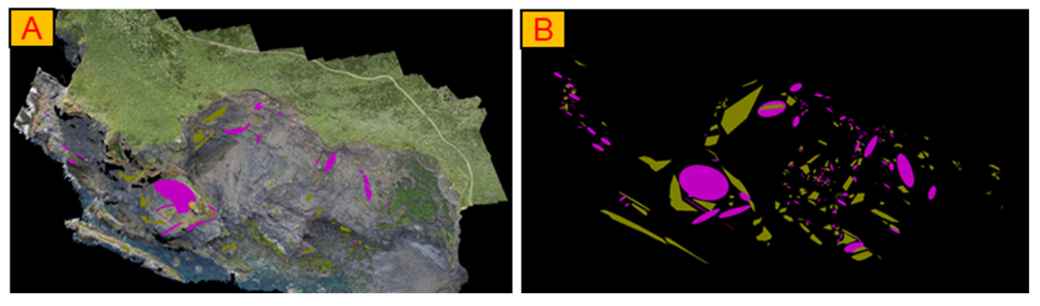
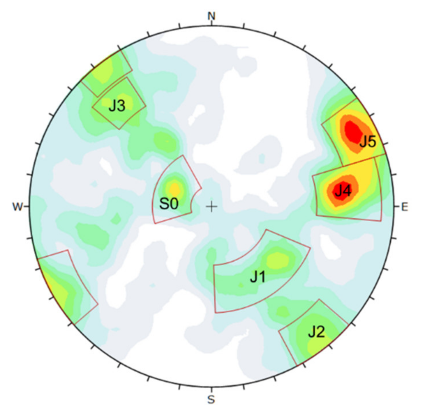
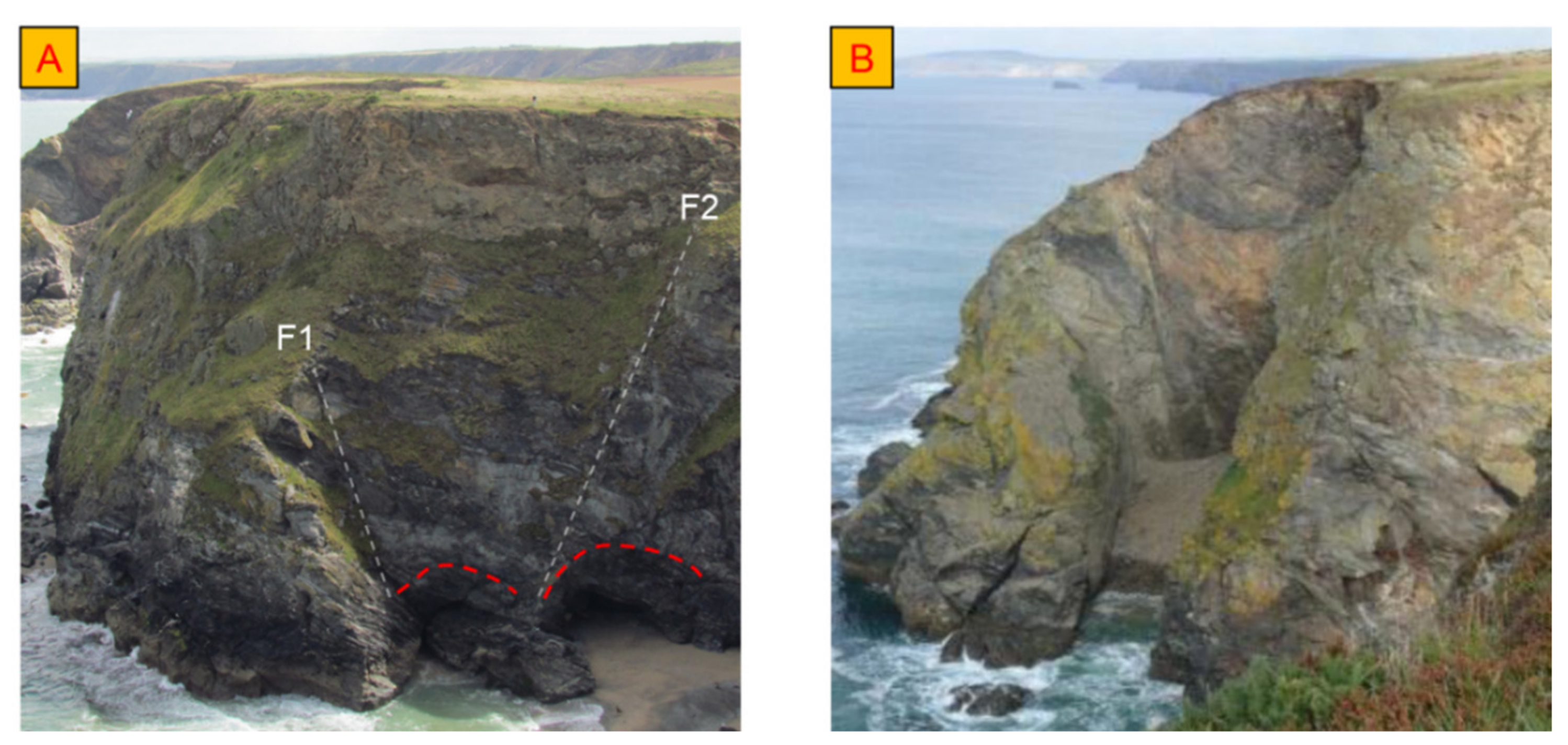
3.2. Geological Structure Extraction from Remote Sensing Surveys

The high risk involved in accessing steep coastal slopes dramatically increases the difficulty of undertaking field surveys by means of conventional methods. Therefore, it was determined that remote sensing techniques were a more appropriate solution to detect geological structures of a representative slope within the study area (at Hell’s Mouth). In this study, UAV photogrammetric and aerial LiDAR surveys were combined to provide a basis for geological structure extraction. The photogrammetric survey was implemented in an oblique manner to obtain images of the steep and high coastal cliff. Due to its high performance in terms of accuracy, vegetation penetration and robustness against geometric distortions, aerial LiDAR provides appropriate detection of geological structures daylighted on the slope surface.

A Panasonic DMC-GH4 camera on a UAV was used to capture overlapped stereo images (resolution: 4608 × 3456). From the UAV photogrammetric survey, a point cloud was constructed using the structure from motion algorithm by using Metashape software [35], and georeferenced by eight GCPs that were derived from 180 corrected observations using Trimble R10 RTK GNSS. In addition, another LiDAR point cloud with a 1 m grid resolution was collected from the Channel Coastal Observatory [36] for complementary use. The software Split FX was adopted to load the point cloud, through which fracture ‘patches’ were manually identified by fitting collections of triangles that conform to a flatness criterion. Orientations of the fracture traces derived from patches were then extracted [37]. The method used has been explained in many case studies [38,39]. A greater number of discontinuities could be obtained by defining the discontinuity sets with the combination of features identified from the two point clouds (Figure 3).

Six discontinuity sets were recognized over the study, as presented in Figure 4 and

Table 1. Properties of six discontinuity sets identified through remote sensing surveys, including dip angle, dip direction, and some descriptions associated with the surface conditions obtained from [22].

Joint Set	Dip (°) / Dip Direction (°)	Description
S0	26/114	Bedding. Smooth, undulating, planar.
J1	51/309	Rough, undulating, stepped.
J2	90/322	Smooth, undulating, planar.
J3	74/141	Rough, undulating, planar.
J4	70/264	Smooth, undulating, planar.
J5	84/242	Smooth, undulating, planar.

. They mainly followed two trends (NW–SE and NE–SW) and have a potential contribution to the geological evolution of the area, as the trends of the discontinuity sets coincide with the predominant trends of the evolution. Bedding (S0) was slightly tilted, with the highest persistence among the identified discontinuity sets. The joints in S3 have a dip direction parallel to the bedding, but were highly tilted. Joint sets J2 and J5 were sub-vertical and have a dip direction sub-orthogonal to each other. Joint set S1, with the lowest persistence, was sub-parallel to J2. It is likely that J4 and J5 are subsets of the same features, but were included separately for analysis purposes.

3.3. Variables Associated with Geometric Conditions, Sea Erosion and Geological Conditions

Given that the case study area was a section of coast, the major influencing factors leading to spatial variation of the landslides shown in Figure 2 were mainly concerned with geological conditions, geometric conditions of slopes, and sea erosion conditions.

Aspect, profile and plan curvature, slope, and cliff height, as prominent factors, have frequently been adopted to assess geometric conditions of slopes [8,9,19,40,41]; in the context of coastal landslides, distance from sea was adopted to assess sea erosion conditions [42,43]; the material of the bedrocks has been applied as a representative feature of geological conditions [13,18,44], since it influences rock mass strength with different compressive strength and material constant according to the Hoek-Brown criterion [45]. Their relationship with landslides is illustrated in

Table 2. Selected input variables associated with geometric conditions, sea erosion conditions and geological conditions, and the description of their relationship with landslides.

Category	Variable	Description
Geometric conditions	Aspect	Aspect is the dip direction of slopes, and used to analyze effects of weather/sea conditions (such as wind directions) or unfavorable orientations of discontinuities
	Profile curvature	Two types of curvatures indicate the amount of overburden on a failure plane (convex terrain of slope surface could result in more overburden than concave terrain
	Plan curvature
	Slope angle	Slope angle indicates the potential for kinematic failures of slopes together with unfavorable orientated discontinuities
	Cliff height	As the slope height increases, the shear stress within the toe of the slope increases due to added weight
Sea erosion conditions	Distance from sea	Distance from sea partially characterizes the conditions of sea erosion, which may cause physical and chemical change of coastal slopes, such as the removal of mass on the lower part, providing increases in the shear stress of the slopes and thus decreases in the factor of safety
Geological condition	Material of bedrock	This component influences the shear strength of a rock mass

. These commonly used factors were brought into ML models as input variables for landslide prediction.

The input variables associated with geometric conditions were derived from the 1 m LiDAR DEM data; distance from sea was measured through the distance between a coastline and slope in a satellite image, which can characterize the sizes of the beaches between the sea and the slope. The material of the bedrock was obtained from a 1:50,000 scale geological map from the open-source Digimap database [34].

3.4. Variables Associated with Discontinuities

To incorporate discontinuities into ML landslide analysis, kinematic analysis was applied to estimate places prone to rock slope failures caused by unfavorably orientated discontinuities. In conventional kinematic analysis, a specific slope with a uniform direction is considered. However, this causes it to be inapplicable for characterizing large areas in which the orientations of the slope faces vary considerably [22].

To solve this limitation, GIS-based kinematic analysis similar to that used by Yilmaz et al. [46] and Francioni et al. [22] was adopted within a GIS framework. In the context of GIS-based kinematic analysis, structures were determined to assess the potential of slopes with variable orientations to landslides. Therefore, mathematical representations of the criteria of kinematic failures are required to substitute the conventional stereonet analysis. The GIS-based kinematic analysis was executed within ESRI’s ArcGIS platform and followed rock failure conditions proposed by Hoek and Bray [47].

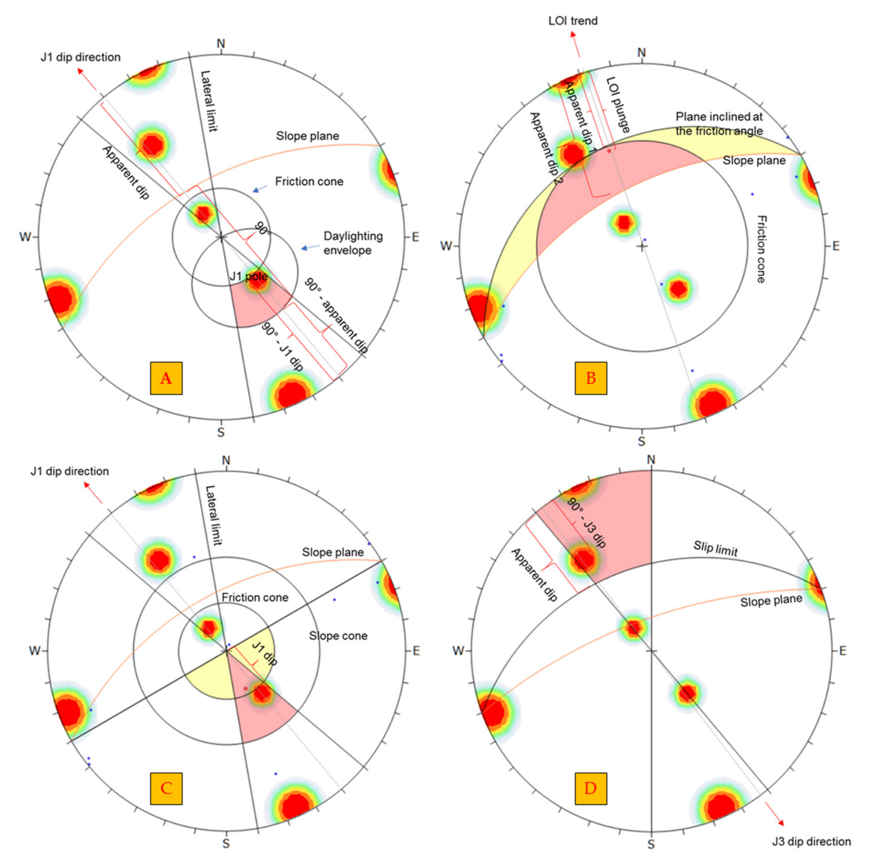
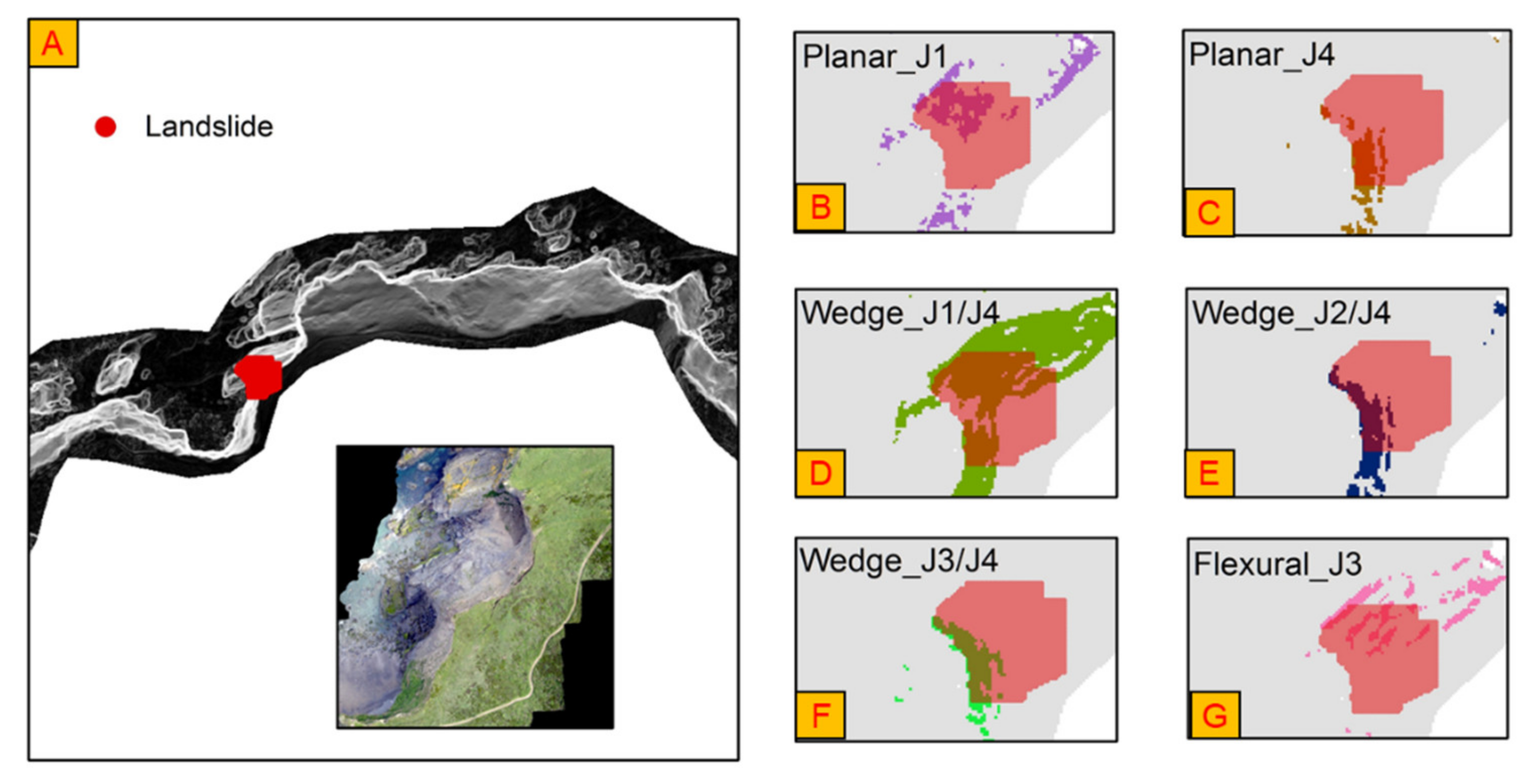
3.4.1. Planar Sliding Kinematic Analysis

Planar rock slope failure occurs when a mass of rock in a slope slides down and along a relatively planar failure surface. In conventional kinematic analysis, the criteria for planar instability are: (1) Dip of failure plane must be greater than angle of friction, so as to exceed the shear strength of the discontinuity; (2) Dip of failure plane must be less than dip of slope face, so as to ‘daylight’ in the slope face; (3) Strike of failure plane must strike parallel to slope crest.

In GIS-based kinematic analysis, a slope prone to planar failure has to meet the requirements associated with the strength, daylighting and orientation conditions as follows (presented in Figure 5A):

• The dip of the major discontinuity is greater than the friction angle (30° was assumed for the mixture of sandstone and mudstone [48]).
• The apparent dip of a slope as seen from the dip direction of the critical discontinuity plane is greater than the dip of the discontinuity plane to allow the discontinuity to daylight on the slope face.
• The slope must be dipped in the same direction as the critical discontinuity plane (a lateral limit of 20° was assumed).

Figure 5. Graphic representation of GIS-based kinematic stereonet analysis to evaluate the potential of a slope for different modes of instability, including (A) planar, (B) wedge, (C) direct toppling, and (D) flexural toppling failures.

Figure 5. Graphic representation of GIS-based kinematic stereonet analysis to evaluate the potential of a slope for different modes of instability, including (A) planar, (B) wedge, (C) direct toppling, and (D) flexural toppling failures.

3.4.2. Wedge Sliding Kinematic Analysis

Wedge sliding kinematic analysis is a test for the sliding of the wedge formed by the intersection of two planes. The wedge block can either slide along the line of intersection (LOI) or a single plane, depending on their orientations. This can be established by stereonet analysis in which the primary and secondary critical zones represent different sliding modes (Figure 5B). The primary critical zone for wedge sliding is the crescent-shaped area (red zone), in which a wedge slides along the LOI or a single plane. The secondary critical zone for wedge sliding is the area between the slope plane and a plane (great circle) inclined at the friction angle (yellow zone), in which LOIs are inclined less than the friction angle, but sliding takes place on a single joint plane that has a dip vector greater than the friction angle.

In GIS-based kinematic analysis, a slope prone to wedge instability in the primary critical zone is required to meet the condition that the apparent dip of a slope as seen from the dip direction of the critical discontinuity is greater than the LOI plunge, which is higher than the friction angle (apparent dip > LOI plunge > friction angle). A slope prone to wedge instability in the secondary critical zone should meet the requirement that the LOI plunge is located between the apparent dip of a slope plane and the apparent dip of the friction angle plane (apparent dip of a slope > LOI plunge > apparent dip of friction angle plane).

3.4.3. Direct Toppling Kinematic Analysis

Direct toppling is a normal rock instability mechanism in which near vertical intersections dip into the slope and near horizontal base planes undercut the blocks and form release planes. The key elements of direct toppling analysis are:

• Two joint sets intersect such that the intersection lines dip into the slope and can form discrete toppling blocks.
• A third joint set exists that acts as a release plane or a sliding plane, allowing the blocks to topple.

As graphically illustrated in the stereonet direct toppling analysis presented in Figure 5C, the pole of the third joint set falls in the red cone whose angle is equal to the slope angle, but also the LOI of two joints falls in the red (direct toppling) or yellow zone (oblique direct toppling).

In GIS-based kinematic analysis, a slope prone to direct toppling instability must meet the requirements associated with the LOI of two intersecting sets as well as the sliding joint set. With respect to the joint set as a sliding plane, the slope should satisfy the following conditions:

• The dip of the slope is greater than the dip of the discontinuity plane.
• The slope dips in the same direction as the discontinuity plane (a lateral limit of 20° was assumed).

As to the LOI, the conditions for the slope are: The slope dips in the same direction as the LOI trend (a lateral limit of 20° was assumed) (primary critical zone for direct toppling), or the slope fails to dip in the same direction as the LOI trend, but falls within a 90° deviation (secondary critical zone for oblique direct toppling).

For oblique direct toppling, the LOI must fall within the friction cone, which requires that the LOI plunge needs to be greater than the ‘90° — friction angle’.

3.4.4. Flexural Toppling Kinematic Analysis

Flexural toppling failure is one of the specific modes of toppling failure that occurs due to bending stresses. For flexural toppling, the critical zone for toppling is defined by the region (see Figure 5D) that falls outside the slip limit plane and inside the lateral limits. The slip limit plane is not an actual physical plane, although it is derived from the slope angle and friction angle. The dip angle of the slip limit plane is derived from the ‘slope dip − friction angle’. The dip direction of the slip limit plane is equal to that of the slope face.

In the context of GIS-based kinematic analysis, a slope prone to flexural toppling instability must meet the following requirements:

• The dip of the slope is greater than the friction angle (30° was assumed).
• The apparent dip of the slip limit plane as seen from the dip direction of a critical discontinuity plane is greater than ‘90°− dip of the critical discontinuity plane’.
• The slope dips in the opposite direction to the critical discontinuity plane (a 20° lateral limit was assumed).

In GIS-based kinematic analysis, the apparent dip is used to calculate the distance of the great circle of the slope plane from the stereonet perimeter in the apparent dip direction in the stereonet analysis (see Figure 5). Apparent dip is calculated as follows:

$$\alpha =arctan\left(sin\beta \times tan\delta \right)$$

(1)

where $\alpha$ is apparent dip; $\delta$ is the real dip of the slope plane; $\beta$ is the angle between the strike direction of the slope plane and the apparent dip direction.

Mechanisms potentially involved in previous landslides within the study area are listed in

Table 3. Slope failure criteria associated with different rock instability mechanisms, in which a is slope apparent dip, d is slope dip direction, $\mathsf{\delta }$ is slope real dip, and ${\mathrm{a}}_{\mathrm{s}}$ is the apparent dip of the slip limit plane for flexural toppling analysis.

Mechanism		Joint Set	Dip/DD (Plunge/Trend)	Failure Criteria
Planar	P1	J1	51°/309°	$\mathrm{a} \ge 51°, d\in \left(309°\pm 20°\right)$
	P2	J4	70°/264°	$\mathrm{a} \ge 70°, d\in \left(264°\pm 20°\right)$
Wedge	W1	J1/J4	49°/329°	$\mathrm{a} \ge 49°, d\in \left(329°\pm 90°\right)$
	W2	J1/J5	50°/325°	$\mathrm{a} \ge 50°, d\in \left(325°\pm 90°\right)$
	W3	J2/J4	67°/232°	$\mathrm{a} \ge 67°, \mathrm{d}\in \left(232°\pm 90°\right)$
	W4	J3/J4	56°/206°	$\mathrm{a} \ge 56°,\mathrm{d}\in \left(206°\pm 90°\right)$
	W5	J4/J5	54°/324°	$\mathrm{a} \ge 54°, d\in \left(324°\pm 90°\right)$
Direct toppling	DT1 (oblique)	Sliding: J1	51°/309°	$\delta \ge 51°, d\in \left(309°\pm 20°\right),$ $d\in \left(351°\pm 90°\right)$
		LOI: J3/J5	72°/171°
	DT2 (oblique)	Sliding: J4	70°/264°	$\delta \ge 70°, d\in \left(264°\pm 20°\right),$ $d\in \left(351°\pm 90°\right)$
		LOI: J3/J5	72°/171°
Flexural toppling	F1	J3	74°/141°	$\mathrm{a} \ge 16°, d\in \left(321°\pm 20°\right),$ $\delta \ge 50°$

. It is suggested that failure mechanisms W1/W2/W5, P1/DT1, and P2/DT2, respectively, were similar failure criteria, causing close results in the kinematic analysis for each group. To reduce complexity, representative mechanisms (W1, P1 and P2) were selected from each group, meaning that W2, W5, DT1 and DT2 were not included in the kinematic analysis. This means that mechanisms P1 (planar failure associated with J1), P2 (planar failure associated with J4), W1 (wedge failure associated with J1/J4), W3 (wedge failure associated with J2/J4), W4 (wedge failure associated with J3/J4), and F1 (flexural toppling failure associated with J3) were considered in the GIS-based kinematic analysis for further landslide prediction.

Kinematic analysis estimated the possibility of each pixel being prone to landslides through a binary classification (yes/no), without consideration of their subsequent effects on local slope stability. To consider local effects, the binary results of the kinematic analysis were converted into density maps (Figure 6). The density was calculated in ArcMap software by counting the number of points (pixels) that were prone to instability in a circle with a 50 m radius. The unit was the number of points/square meter. The input variables provided by GIS-based kinematic analysis were labeled with Planar_J1, Planar_J4, Wedge_J1/J4, Wedge_J2/J4, Wedge_J3/J4, and Flexural_J3 to represent associated failure modes.

3.5. ML Analysis

ML models were used to statistically simulate the relationship of landslides and the input variables. Models were constructed and trained using the training set. Modeling of each ML algorithm returned results of variable importance. Variable importance revealed the significance of each input variable with respect to the dependent variables (0/1 for landslide presence/absence). After the models were constructed, their learning and predictive ability was assessed through the Confusion Matrix and Receiver Operating Characteristic (ROC) curves. These assessments were implemented using the validation set. Two series of ML modeling were carried out. The initial series of modeling was based on the seven commonly used input variables. In addition, a second series of modeling with the inclusion of the discontinuity-related variables was undertaken to make a comparative study.

The predictive capabilities of the two models were assessed on the basis of the confusion matrix and the ROC curve. The confusion matrix was used to assess model performance with respect to their binary classification capability (prediction of landslide absence/presence, 0/1), and the ROC curve was used to evaluate their capability with respect to landslide susceptibility mapping (probability of landslide occurrence).

In this paper, two conventional ML algorithms (RF and SVM) and two neural network algorithms (MLP and DLNN) were adopted, and modeling was performed in a Python environment.

3.5.1. Random Forest

RF, an ensemble algorithm, is comprised of decision trees using bootstrap aggregating methods [1]. The results from the constitutive decision trees in a random forest are aggregated to produce a prediction. The predictive ability of an RF model is sensitive to two parameters: the number of tress (ntree) in the RF and the number of variables for the selection in each node (mtry) of a decision tree [49]. Thus, in this research RF modeling was carried out after tuning these two parameters.

3.5.2. Support Vector Machine

SVM has been widely used for classification objectives. The algorithm attempts to fit a hyperplane in an N-dimensional space (N—the number of variables) that distinctly classifies the data points. In this case study, landslide prediction parameter tuning was conducted on the regularization parameter (C) and kernel type used in the algorithm.

3.5.3. Multilayer Perceptron

A multilayer perceptron (MLP) is a class of feedforward artificial neural network (ANN). Its architecture consists of at least three layers: an input layer, a hidden layer, and an output layer. Each node in the hidden and output layer produces an output through a nonlinear activation function with updated weights. The update of weight is adjusted through a learning algorithm.

The performance of the MLP model is sensitive to the activation function applied to the nodes that defines their outputs, the number of nodes in the hidden layer, and the selection of learning patterns for weight optimization [13]. Therefore, these hyperparameters were tuned to obtain an optimal MLP model.

3.5.4. Deep Learning Neural Network

A deep learning neural network is a class of neural network with considerable depth. It normally consists of an input layer, several hidden layers, and an output layer. The configuration rules of DLNN architectures will not be explained here, as these have been repeatedly presented in many papers [13,17]. In this paper, a DLNN model was used to implement landslide analysis. In the model, the Rectified Linear Unit (ReLU) activation function was applied for nodes in hidden layers to produce outputs. As landslide prediction can be a binary classification, the sigmoid transfer function was used in the output layer to produce a prediction. The Binary Cross-Entropy loss function was used to estimate the loss of the model so that the weights of nodes could be updated and optimized to obtain an optimal model.

During the configuration of a DLNN model, some hyperparameters have a significant influence on its performance, including (1) the number of hidden layers; (2) the number of nodes in each layer; (3) the selection of an optimization algorithm; and (4) learning rate. Thus, these hyperparameters were tuned to obtain an optimal DLNN model for landslide analysis.

3.6. Frequency Ratio Analysis

FR analysis was carried out to quantitively explore the relationship between landslides and the input variables associated with kinematic analysis by using the data acquired from training and validation sets. The analysis assigned a weight coefficient to each class of analyzed input variables. The weight coefficient expresses the probabilistic relationship of the class and landslides.

To obtain the RF values (weight coefficient) the following equations were used:

$$F{R}_i\left(j\right)=\frac{a_i\left(\mathrm{j}\right)}{b_i\left(\mathrm{j}\right)}$$

(2)

$$a_i\left(\mathrm{j}\right)=\frac{L{S}_i\left(j\right)}{LS}$$

(3)

$$b_i\left(\mathrm{j}\right)=\frac{P_i\left(j\right)}{P}$$

(4)

where $L{S}_i\left(j\right)$ is the number of pixels containing landslides in a class j of variable i; LS is the total number of pixels containing landslides; $P_i\left(j\right)$ is the total number of pixels of class i of variable j in the whole area; P is the total number of pixels in the whole area. In this research, P is 1020 and LS is 510.

4. Results

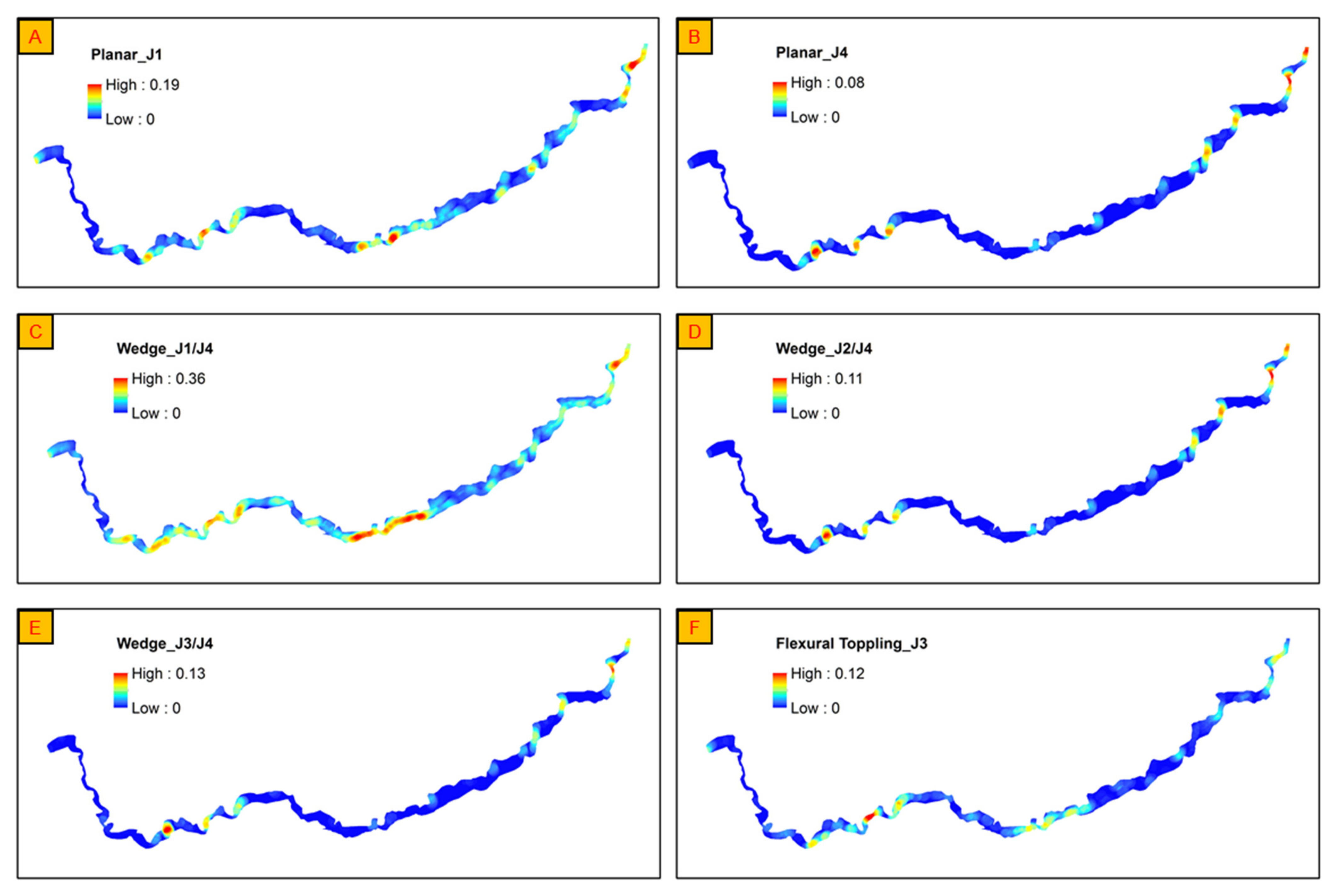
4.1. Frequency Ratio Analysis

In FR analysis, the analyzed variables related to kinematic analysis were categorized into three different classes in accordance with their density values. On the basis of the results of FR analysis (

Table 4. The results of FR analysis of the discontinuity-related factors, including Planar_J1, Planar_J4, Wedge_J1/J4, Wedge_J2/J4, Wedge_J3/J4, and Flexural_J3.

Mechanism	Class	LSi	ai	Pi	bi	FR
Planar_J1	Class 1: [0, 0.05]	156	0.31	573	0.56	0.54
	Class 2: (0.05, 0.1]	213	0.42	283	0.28	1.51
	Class 3: (0.1, max]	141	0.28	164	0.16	1.72
Planar_J4	Class 1: [0, 0.02]	242	0.47	721	0.71	0.67
	Class 2: (0.02, 0.04]	109	0.21	123	0.12	1.77
	Class 3: (0.04, max]	159	0.31	176	0.17	1.81
Wedge_J1/J4	Class 1: [0, 0.1]	69	0.14	359	0.35	0.38
	Class 2: (0.1, 0.2]	208	0.41	364	0.36	1.14
	Class 3: (0.2, max]	233	0.46	297	0.29	1.57
Wedge_J2/J4	Class 1: [0, 0.03]	261	0.51	742	0.73	0.70
	Class 2: (0.03, 0.06]	119	0.23	132	0.13	1.80
	Class 3: (0.06, max]	130	0.25	146	0.14	1.78
Wedge_J3/J4	Class 1: [0,0.03]	307	0.60	794	0.78	0.77
	Class 2: (0.03, 0.06]	93	0.18	101	0.10	1.84
	Class 3: (0.06, max]	110	0.22	125	0.12	1.76
Flexural_J3	Class 1: [0, 0.03]	271	0.53	726	0.71	0.75
	Class 2: (0.03, 0.06]	188	0.37	233	0.23	1.61
	Class 3: (0.06, max]	51	0.10	61	0.06	1.67

), a common distribution characteristic for all analyzed variables was revealed. Good consistency was observed between FR values and class values, whereby classes with high values possessed high FR values. In addition, quantitatively, most pixels in class 2 and class 3 are landslides points, but pixels in class 1 are mostly non-landslides points. Taking Planar_J4 as an example, 479 in 721 pixels in class 1 are non-landslide points, while 109 in 123 pixels and 159 in 176 pixels in class 2 and class 3, respectively, are landslide points.

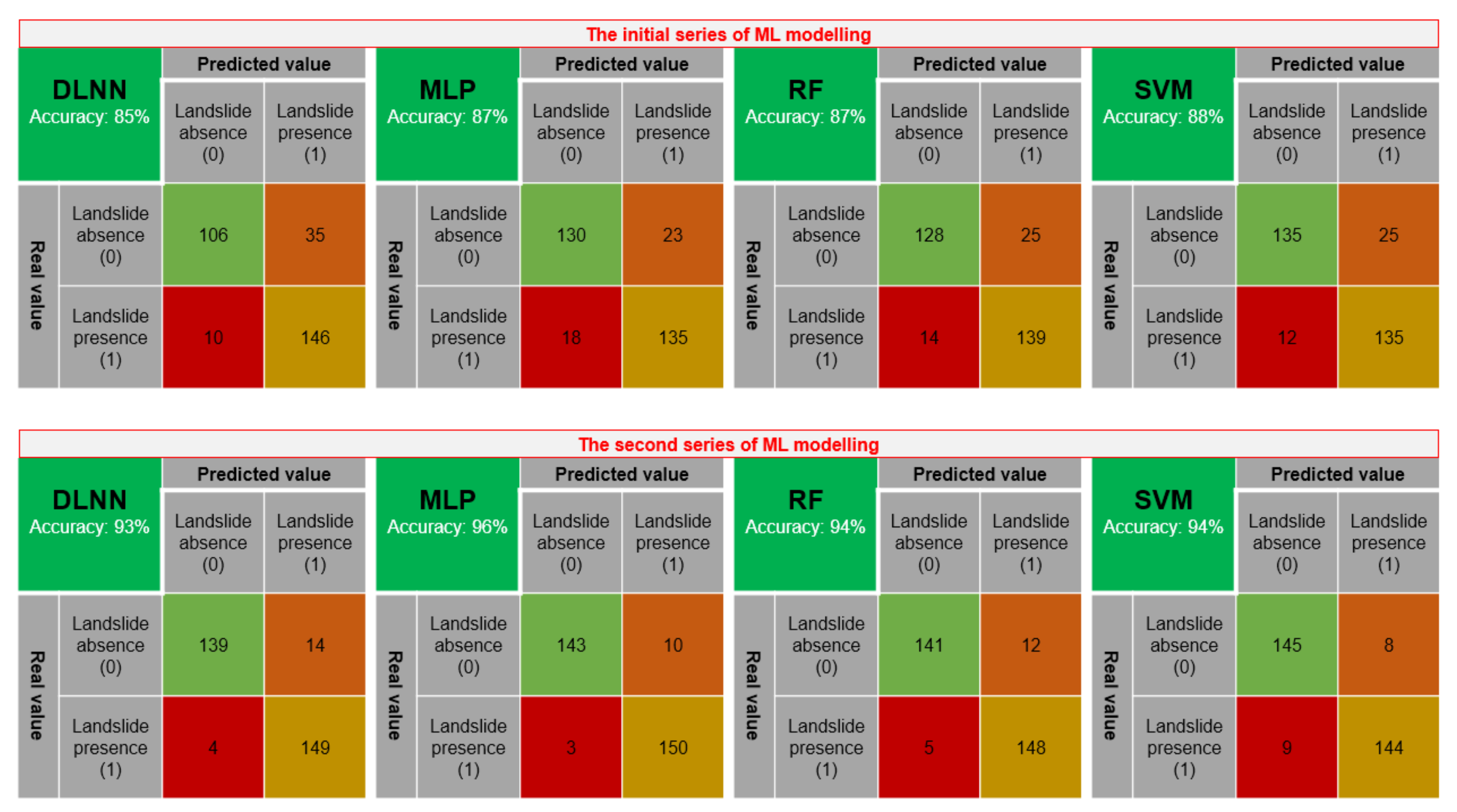
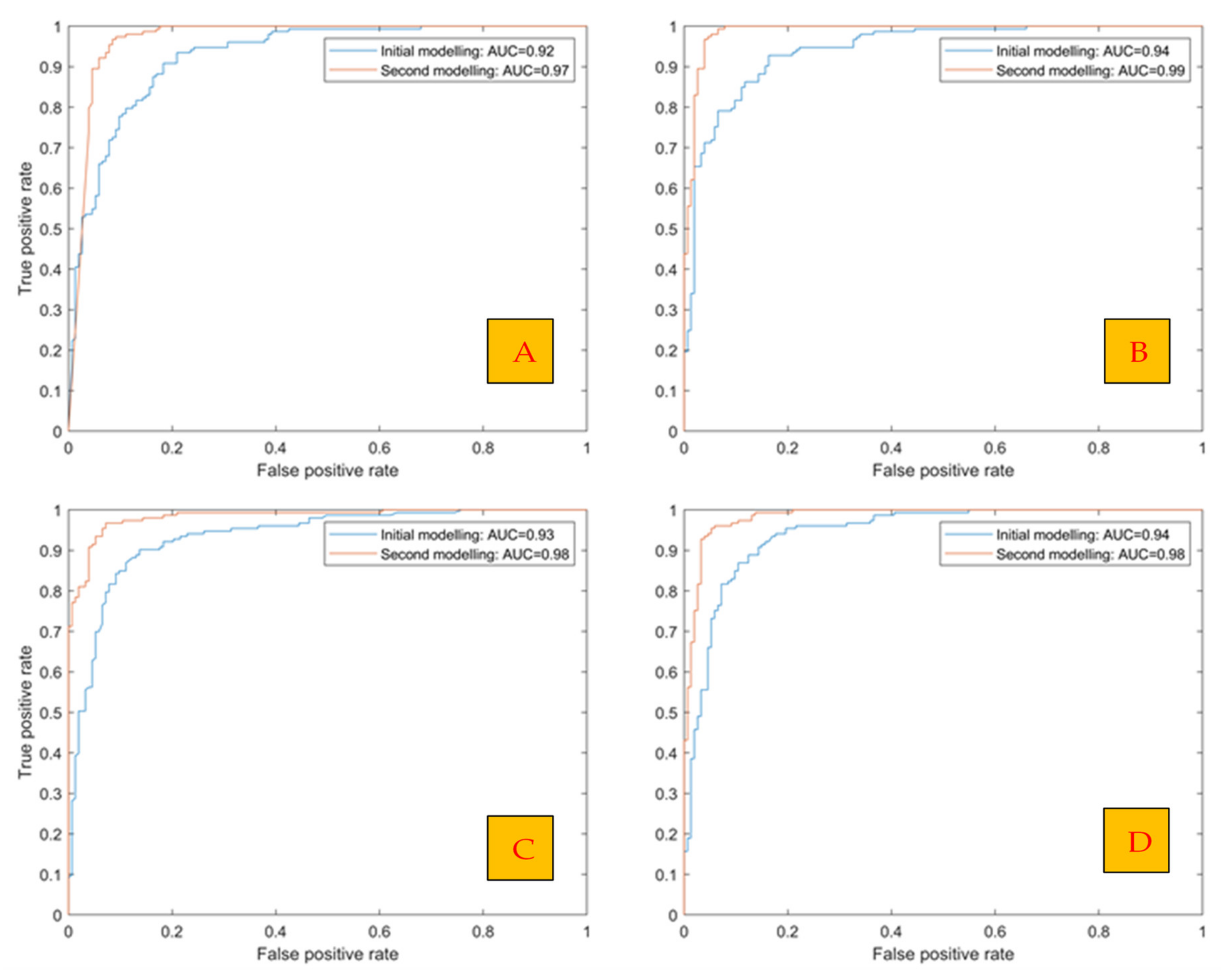
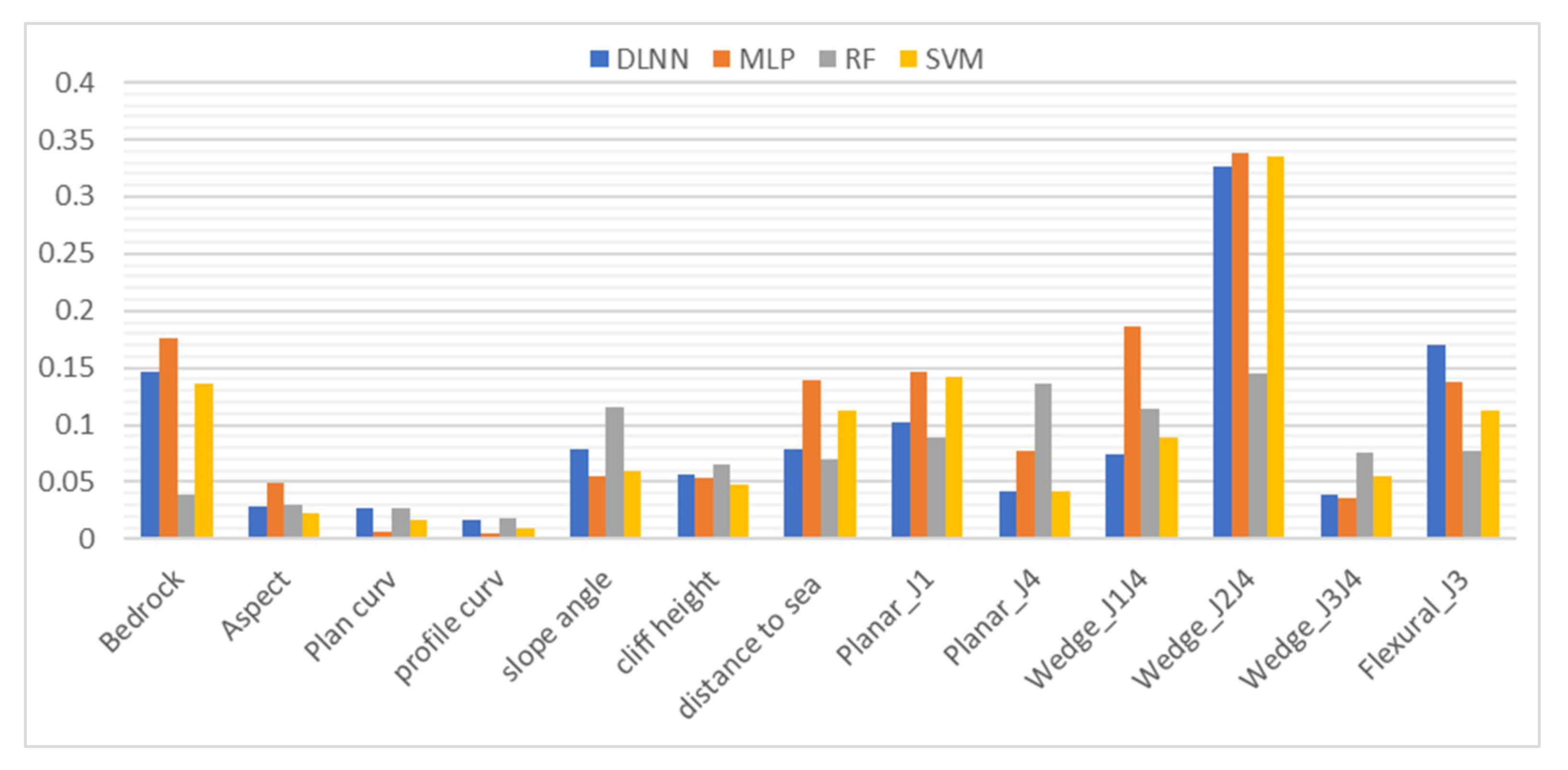
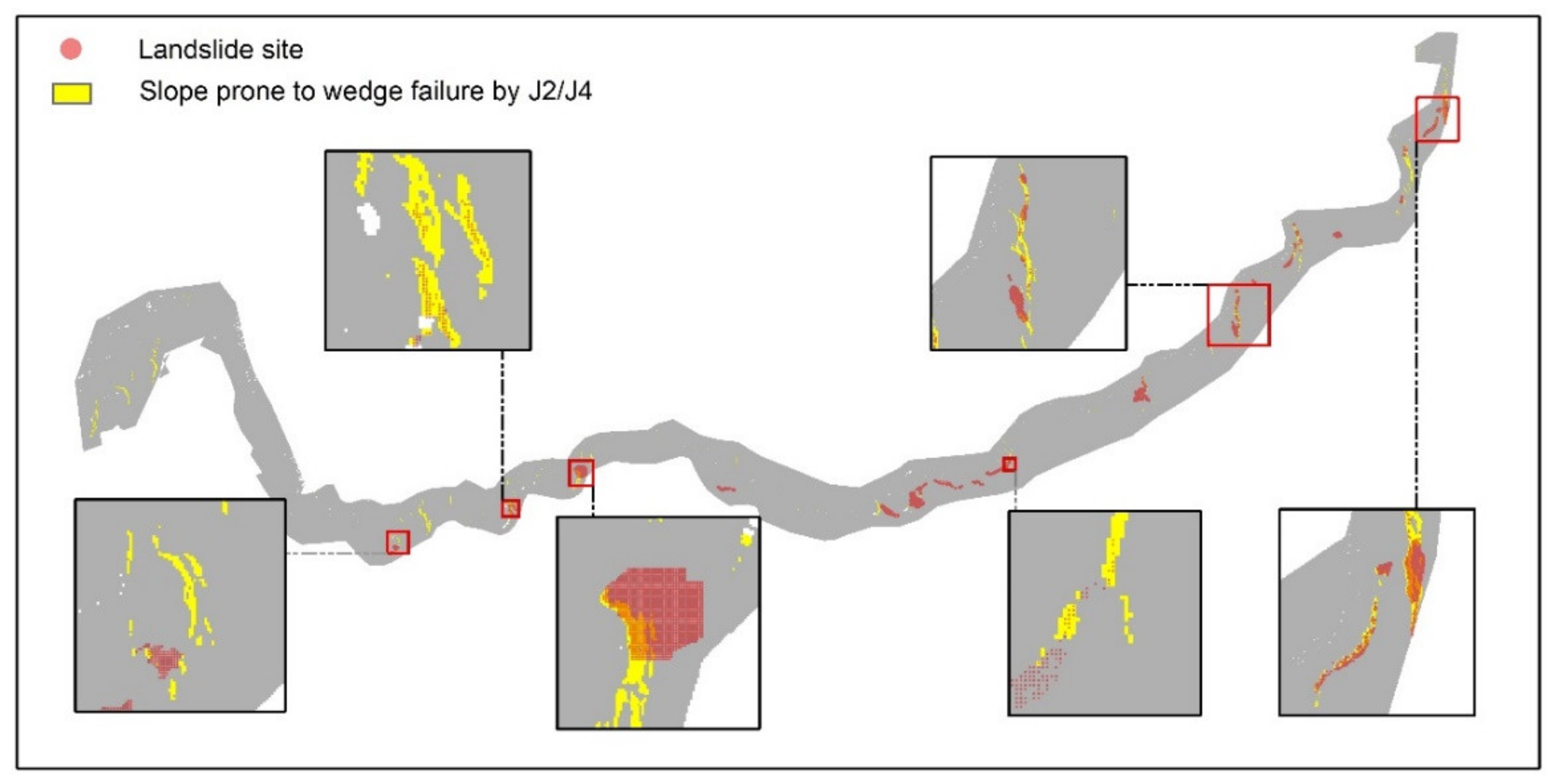
4.2. Machine Learning Analysis

Parameter tuning was carried out using several trial and error runs to obtain the most accurate prediction and to optimize the hyperparameters of the ML models involved in the initial (without discontinuity-related variables) and second series (with discontinuity-related variables) of modeling. The parameters in the initial (second) modeling were tuned as below:

• For the RF model, ntree was assigned as 500 (500), and mtry was 3 (4).
• For the SVM model, the kernel was specified as the radial basis function (‘rbf’), and the regularization parameter C was assigned as 100 (100).
• For the MLP model, the activation function was specified as being ‘logistic’ (‘logistic’); the weight optimization algorithm was specified as ‘lbfgs’ (‘lbfgs’); the regularization parameter alpha was assigned as 0.1 (0.1); 10 (9) nodes were contained in the hidden layer.
• For the DLNN model, a Keras sequential model with 3 (3) hidden layers was configured. Each layer contained 64 (128) neurons. The optimizer used in this model was ‘Adadelta’ for the adaptive learning rate. An EarlyStopping callback was used in conjunction with model training to save optimal epoch the batch size of 1 to prevent overfitting.

The assessment results of classification capability using the confusion matrix are presented in Figure 7. From the perspective of ‘vertical comparison’, the integration of discontinuity-related input variables significantly reduces cases of the misclassification of landslide absence (0) as well as landslide presence (1). This is also reflected by the increase in overall classification accuracy, from 85% to 93% for DLNN modeling, from 87% to 96% for MLP modeling, from 87% to 94% for RF modeling, and from 88% to 94% for SVM modeling.

The assessment results of LSM capability by ROC curves are presented in Figure 8. Comparative analysis of the curves from the two modeling series shows that with respect to each model, the curve obtained from the initial modeling overrides that from the second modeling. This distribution characteristic is confirmed by the higher AUC values obtained for the initial modeling.

The ML analysis provides a variable importance analysis, as shown in Figure 9. The importance indicates the importance of each variable to landslide prediction in the initial modeling. For all four of the models selected, the discontinuity-related input variable Wedge_J2/J4, obtained from GIS-based kinematic analysis, exclusively takes the highest importance among the 13 variables.

5. Validation and Discussion

In this research, discontinuities were introduced into ML-based landslide prediction as a controlling factor of rock mass instability by using the method of GIS-based kinematic analysis. The analysis assessed the potential of slopes to be prone to kinematic instabilities, including planar, wedge, direct toppling, and flexural toppling instability modes. GIS-based kinematic analysis is likely to provide effective clues to future landslide occurrence. Figure 10 highlights six regions prone to wedge failures caused by J2/J4, which coincide with locations of previous landslides occurring in the study area. The highlighted landslides have a similar direction, dipping toward W or WNW. Some other landslides in slopes dipping towards N or NNW in the middle of the study area are proposed to be influenced by planar sliding kinematic analysis associated with J1 and wedge sliding kinematic analysis associated with J1/J4 (see Figure 6).

In addition, there was a catastrophic landslide in 2011 in the study area with an estimated volume of 100,000 m³ (Hell’s Mouth landslide) [22]. By using the data in 2008, the GIS-based kinematic analysis effectively indicates the risk of possible kinematic failures at this location (Figure 11). The analysis is a result of binary classification that indicates the unstable condition of the slope toe and the stable condition of the slope crown. If the binary results (0/1) were to be applied as input variables in machine learning models, they would provide misleading information at the slope crown, where instability occurred. However, density mapping, transformed from binary classification, solved this problem by accounting for the unstable points in a 50 m circle range, considering that toe removal may trigger the development of instability at the slope crown (namely local effects).

The result of FR analysis provided evidence to support the effects of the GIS-based kinematic analysis. The results showed that high FR values only appear in the classes with high density (class 2 and 3), with respect to variables obtained from kinematic analysis. In addition, quantitively, most pixels in class 2 and 3 are landslides points, and most pixels in class 1 are non-landslide points. These distribution characteristics indicate that discontinuity-related factors with high density are likely to be an indicator of landslide occurrence.

With the inclusion of discontinuity-related variables, the landslide prediction accuracy of the four ML models improved dramatically, which is supported by the results of the two validation methods (Figure 7 and Figure 8). The increase in prediction accuracy was due to the decrease in the misclassification rate of landslide absence cases as well landslide presence cases. The contrasting predictive capability highlights that these discontinuity-related variables are essential for landslide prediction. The results of variable importance analysis, showing that the factor Wedge_J2/J4 is the most important variable in ML landslide analysis, also supports the above conclusion.

However, the results of the kinematic analysis cannot be used as a standalone criterion for landslide prediction, since it only considers the influences of unfavorable orientations of discontinuities. Without consideration of some other factors, such as rock mass strength and sea erosion conditions, kinematic analysis is likely to overestimate the extent of slopes prone to coastal rock landslides in this study. This overestimation is reflected in Figure 10, where some stable slopes are misclassed as unstable ones. From this perspective, in ML modeling, variables associated with bedrock, geometric conditions and sea erosion conditions potentially act as limiting conditions to refine landslide prediction by kinematic analysis.

Although less important than discontinuity-related variables in ML modeling, the variables related to bedrock, geometric conditions and sea erosion conditions may facilitate the occurrence of landslides and contribute to the landslide prediction. For example, the distance from the sea shows reasonable importance for landslide prediction, potentially indicating that different distances from the sea could result in various stability conditions. Slopes with less distance from the sea likely have more opportunity to interact with the sea and waves; therefore, they are more likely to be prone to sea erosion. It has been evidenced that the formation of a gully at Hell’s Mouth was pre-conditioned by erosion-induced sea caves, on which discontinuities could be daylighted and stress from overburden concentrated. Finally, a gully formed as a result of these conditions (Figure 12). Another important variable is the material of the bedrock. The bedrock map shows that the Porthtowan Formation is more prone to landslides (Figure 13), potentially due to the conditions of the rocks (metamudstone and mudstone/mudstone and sandstone) in the Porthtowan Formation being conducive to landslides with respect to the geometrical arrangement of outcrops, strength, weathering, grain size, etc. However, individual variables/factors would not solely trigger landslides, but rather would interact with each other to reduce the strength of rock masses, consequently resulting in instability.

This paper provides guidelines for the generalization of the proposed method to other regions in order to perform extensive rock slope stability surveys. This can be implemented by incorporating local discontinuity information into machine learning modeling, including the detection of local discontinuities using remote sensing techniques, the processing of the discontinuity data through GIS-based kinematic analysis for the assessment of slopes prone to different modes of instability, the digitalization of the results of GIS-based kinematic analysis from binary classification to continuous values that are more applicable to ML models, and the combined use of discontinuity-related variables and other appropriate landslide preconditioning factors to train ML models and predict landslides.

It is noteworthy that even without the involvement of discontinuity-related factors, the prediction accuracy of ML models based on the seven common factors was still rather high, achieving approximately 87% of ACC and 0.94 of AUC. This is likely caused by the high sampling density of 30 pixels being selected from each landslide site. The 30 pixels from same site will potentially have had similar characteristics, such as similar bedrock material. The 70%:30% strategy for splitting the acquired data for model construction and model validation means that the validation data, to some extent, will resemble the training data, which could cause the high prediction accuracy. However, the involvement of discontinuity-related variables was still able to improve the prediction accuracy to a higher level, which demonstrates the reliable application of these variables in ML-based landslide prediction.

6. Conclusions

Discontinuities, and especially their orientations, have rarely been considered in ML landslide prediction. In this context, this paper proposes a novel application of unfavorably orientated discontinuities in ML landslide analysis. Six discontinuity sets were detected within the study area through photogrammetric and aerial LiDAR surveys. These structural features were applied to assess the potential of slopes to be prone to different modes of rock instability (planar, wedge, direct toppling, and flexural topping) by GIS-based kinematic analysis. In order to consider local effects, the binary results of the kinematic analysis were transformed into density maps for subsequent FR analysis and ML analysis. Six density maps were obtained based on the results of GIS-based kinematic analysis associated with different rock instability mechanisms, including planar sliding controlled by J1 and J4, wedge sliding controlled by J1/J4, J2/J4 and J3/J4, and flexural topping controlled by J3. These density variables, as well as some commonly used landslide influencing factors, were then considered as input variables in ML models to predict landslides.

To validate the results of the GIS-based kinematic analysis, comparisons were made with previous landslide sites. The comparison results indicate that the slopes prone to kinematic failures presented in Figure 10 and Figure 11 were identified as the sites of previous landslides. This highlights the reliable application of GIS-based kinematic analysis in landslide prediction.

Good consistency was observed, through FR analysis, between landslide probability, which was characterized by FR values, and discontinuity-related variables, showing that classes with higher values possessed higher FR values. The coincidence with respect to their distribution characteristics indicates a close correlation between them.

The results of model assessment on the basis of confusion matrix and ROC curves showed that the inclusion of discontinuity-related input variables significantly improved the prediction accuracy of the four ML models. In addition, variable importance analysis revealed that discontinuity-related variables took the highest importance in landslide prediction in the four ML models.

The above findings highlight the reliable application of GIS-based kinematic analysis for assessing slopes prone to landslides. In addition, the novel application of unfavorably orientated discontinuities in ML models using GIS-based kinematic analysis improves landslide prediction.

References

1. Dilley, M.; Chen, R.; Deichmann, U.; Lerner-Lam, A.; Arnold, M.; Agwe, J.; Yetman, G. Natural Disaster Hotspots: A Global Risk; The World Bank: Washington, DC, USA, 2005. [Google Scholar]
2. Van Tien, P.; Sassa, K.; Takara, K.; Fukuoka, H.; Dang, K.; Shibasaki, T.; Ha, N.D.; Setiawan, H.; Loi, D.H. Formation process of two massive dams following rainfall-induced deep-seated rapid landslide failures in the Kii Peninsula of Japan. Landslides 2018, 15, 1761–1778. [Google Scholar] [CrossRef]
3. Xu, Y.; George, D.L.; Kim, J.; Lu, Z.; Riley, M.; Griffin, T.; de la Fuente, J. Landslide monitoring and runout hazard assessment by integrating multi-source remote sensing and numerical models: An application to the Gold Basin landslide complex, northern Washington. Landslides 2021, 18, 1131–1141. [Google Scholar] [CrossRef]
4. Gao, Y.; Li, B.; Gao, H.; Chen, L.; Wang, Y. Dynamic characteristics of high-elevation and long-runout landslides in the Emeishan basalt area: A case study of the Shuicheng “7.23”landslide in Guizhou, China. Landslides 2020, 17, 1663–1677. [Google Scholar] [CrossRef]
5. Bolla, A.; Paronuzzi, P. Geomechanical Field Survey to Identify an Unstable Rock Slope: The Passo della Morte Case History (NE Italy). Rock Mech. Rock Eng. 2019, 53, 1521–1544. [Google Scholar] [CrossRef]
6. Yilmaz, I. Comparison of landslide susceptibility mapping methodologies for Koyulhisar, Turkey: Conditional probability, logistic regression, artificial neural networks, and support vector machine. Environ. Earth Sci. 2009, 61, 821–836. [Google Scholar] [CrossRef]
7. Xu, C.; Dai, F.; Xu, X.; Lee, Y.H. GIS-based support vector machine modeling of earthquake-triggered landslide susceptibility in the Jianjiang River watershed, China. Geomorphology 2012, 145-146, 70–80. [Google Scholar] [CrossRef]
8. Kavzoglu, T.; Sahin, E.K.; Colkesen, I. Landslide susceptibility mapping using GIS-based multi-criteria decision analysis, support vector machines, and logistic regression. Landslides 2013, 11, 425–439. [Google Scholar] [CrossRef]
9. Dou, J.; Yunus, A.P.; Bui, D.T.; Merghadi, A.; Sahana, M.; Zhu, Z.; Chen, C.-W.; Khosravi, K.; Yang, Y.; Pham, B.T. Assessment of advanced random forest and decision tree algorithms for modeling rainfall-induced landslide susceptibility in the Izu-Oshima Volcanic Island, Japan. Sci. Total Environ. 2019, 662, 332–346. [Google Scholar] [CrossRef] [PubMed]
10. Behnia, P.; Blais-Stevens, A. Landslide susceptibility modelling using the quantitative random forest method along the northern portion of the Yukon Alaska Highway Corridor, Canada. Nat. Hazards 2017, 90, 1407–1426. [Google Scholar] [CrossRef]
11. Chen, W.; Peng, J.; Hong, H.; Shahabi, H.; Pradhan, B.; Liu, J.; Zhu, A.-X.; Pei, X.; Duan, Z. Landslide susceptibility modelling using GIS-based machine learning techniques for Chongren County, Jiangxi Province, China. Sci. Total Environ. 2018, 626, 1121–1135. [Google Scholar] [CrossRef] [PubMed]
12. Huang, F.; Cao, Z.; Guo, J.; Jiang, S.-H.; Li, S.; Guo, Z. Comparisons of heuristic, general statistical and machine learning models for landslide susceptibility prediction and mapping. Catena 2020, 191, 104580. [Google Scholar] [CrossRef]
13. Bui, D.T.; Tsangaratos, P.; Nguyen, V.-T.; Van Liem, N.; Trinh, P.T. Comparing the prediction performance of a Deep Learning Neural Network model with conventional machine learning models in landslide susceptibility assessment. Catena 2020, 188, 104426. [Google Scholar] [CrossRef]
14. Sameen, M.I.; Pradhan, B.; Lee, S. Application of convolutional neural networks featuring Bayesian optimization for landslide susceptibility assessment. Catena 2020, 186, 104249. [Google Scholar] [CrossRef]
15. Lucchese, L.V.; De Oliveira, G.G.; Pedrollo, O.C. Attribute selection using correlations and principal components for artificial neural networks employment for landslide susceptibility assessment. Environ. Monit. Assess. 2020, 192, 1–22. [Google Scholar] [CrossRef] [PubMed]
16. Liu, Z.; Gilbert, G.; Cepeda, J.M.; Lysdahl, A.O.K.; Piciullo, L.; Hefre, H.; Lacasse, S. Modelling of shallow landslides with machine learning algorithms. Geosci. Front. 2021, 12, 385–393. [Google Scholar] [CrossRef]
17. Nhu, V.-H.; Hoang, N.-D.; Nguyen, H.; Ngo, P.T.T.; Bui, T.T.; Hoa, P.V.; Samui, P.; Bui, D.T. Effectiveness assessment of Keras based deep learning with different robust optimization algorithms for shallow landslide susceptibility mapping at tropical area. Catena 2020, 188, 104458. [Google Scholar] [CrossRef]
18. Chen, W.; Li, Y. GIS-based evaluation of landslide susceptibility using hybrid computational intelligence models. Catena 2020, 195, 104777. [Google Scholar] [CrossRef]
19. Pham, B.T.; Prakash, I.; Singh, S.K.; Shirzadi, A.; Shahabi, H.; Bui, D.T. Landslide susceptibility modeling using Reduced Error Pruning Trees and different ensemble techniques: Hybrid machine learning approaches. Catena 2019, 175, 203–218. [Google Scholar] [CrossRef]
20. Stead, D.; Wolter, A. A critical review of rock slope failure mechanisms: The importance of structural geology. J. Struct. Geol. 2015, 74, 1–23. [Google Scholar] [CrossRef]
21. Ferrero, A.M.; Migliazza, M.R.; Pirulli, M.; Umili, G. Some Open Issues on Rockfall Hazard Analysis in Fractured Rock Mass: Problems and Prospects. Rock Mech. Rock Eng. 2016, 49, 3615–3629. [Google Scholar] [CrossRef]
22. Francioni, M.; Coggan, J.; Eyre, M.; Stead, D. A combined field/remote sensing approach for characterizing landslide risk in coastal areas. Int. J. Appl. Earth Obs. Geoinformation 2018, 67, 79–95. [Google Scholar] [CrossRef]
23. Francioni, M.; Salvini, R.; Stead, D.; Coggan, J. Improvements in the integration of remote sensing and rock slope modelling. Nat. Hazards 2018, 90, 975–1004. [Google Scholar] [CrossRef] [Green Version]
24. Meng, F.; Wong, L.N.Y.; Zhou, H.; Wang, Z. Comparative study on dynamic shear behavior and failure mechanism of two types of granite joint. Eng. Geol. 2018, 245, 356–369. [Google Scholar] [CrossRef]
25. Vatanpour, N.; Ghafoori, M.; Talouki, H.H. Probabilistic and sensitivity analyses of effective geotechnical parameters on rock slope stability: A case study of an urban area in northeast Iran. Nat. Hazards 2014, 71, 1659–1678. [Google Scholar] [CrossRef]
26. Havaej, M.; Wolter, A.; Stead, D. The possible role of brittle rock fracture in the 1963 Vajont Slide, Italy. Int. J. Rock Mech. Min. Sci. 2015, 78, 319–330. [Google Scholar] [CrossRef]
27. Vanneschi, C.; Eyre, M.; Venn, A.; Coggan, J.S. Investigation and modeling of direct toppling using a three-dimensional distinct element approach with incorporation of point cloud geometry. Landslides 2019, 16, 1453–1465. [Google Scholar] [CrossRef]
28. Shail, R.K.; Coggan, J.S.; Stead, D. Coastal landsliding in Cornwall, UK: Mechanisms, modelling and implications. In Proceedings of the 8th International Congress IAEG, Vancouver, BC, Canada, 21–25 September 1998; pp. 1323–1330. [Google Scholar]
29. Leveridge, B.; Shail, R. The Gramscatho Basin, south Cornwall, UK: Devonian active margin successions. Proc. Geol. Assoc. 2011, 122, 568–615. [Google Scholar] [CrossRef] [Green Version]
30. Hollick, L.; Shail, R.; Leveridge, B. Devonian Rift-Related Sedimentation and Variscan Tectonics—New Data on the Looe and Gramscatho Basins from the Resurvey of the Newquay District; The Ussher Society, 2006. Geosci. South-West Engl. 2006, 11, 191–198. [Google Scholar]
31. Turner, D.; Lucieer, A.; De Jong, S.M. Time Series Analysis of Landslide Dynamics Using an Unmanned Aerial Vehicle (UAV). Remote. Sens. 2015, 7, 1736–1757. [Google Scholar] [CrossRef] [Green Version]
32. Maurer, J.; Rupper, S. Tapping into the Hexagon spy imagery database: A new automated pipeline for geomorphic change detection. ISPRS J. Photogramm. Remote. Sens. 2015, 108, 113–127. [Google Scholar] [CrossRef]
33. Kim, M.-K.; Sohn, H.-G.; Kim, S. Incorporating the effect of ALS-derived DEM uncertainty for quantifying changes due to the landslide in 2011, Mt. Umyeon, Seoul. GIScience Remote. Sens. 2019, 57, 287–301. [Google Scholar] [CrossRef]
34. Digimap. Available online: https://digimap.edina.ac.uk/lidar (accessed on 6 February 2021).
35. Agisoft. Metashape; Agisoft LLC: Brooklyn, NY, USA, 2016.
36. Channel Coastal Observatory. Available online: https://www.channelcoast.org/ (accessed on 6 February 2021).
37. Split Engineering LLC. Split-FX. 2016. Available online: https://www.spliteng.com/ (accessed on 6 February 2021).
38. Poluga, S.L.; Shakoor, A.; Bilderback, E.L. Rock Mass Characterization and Stability Evaluation of Mount Rushmore National Memorial, Keystone, South Dakota. Environ. Eng. Geosci. 2018, 24, 385–412. [Google Scholar] [CrossRef]
39. Lato, M.; Diederichs, M.S.; Hutchinson, D.J.; Harrap, R. Optimization of LiDAR scanning and processing for automated structural evaluation of discontinuities in rockmasses. Int. J. Rock Mech. Min. Sci. 2009, 46, 194–199. [Google Scholar] [CrossRef]
40. Wang, Y.; Fang, Z.; Hong, H. Comparison of convolutional neural networks for landslide susceptibility mapping in Yanshan County, China. Sci. Total Environ. 2019, 666, 975–993. [Google Scholar] [CrossRef]
41. Shao, X.; Ma, S.; Xu, C.; Zhang, P.; Wen, B.; Tian, Y.; Zhou, Q.; Cui, Y. Planet Image-Based Inventorying and Machine Learning-Based Susceptibility Mapping for the Landslides Triggered by the 2018 Mw6.6 Tomakomai, Japan Earthquake. Remote. Sens. 2019, 11, 978. [Google Scholar] [CrossRef] [Green Version]
42. Abanades, J.; Greaves, D.; Iglesias, G. Coastal defence using wave farms: The role of farm-to-coast distance. Renew. Energy 2015, 75, 572–582. [Google Scholar] [CrossRef] [Green Version]
43. Levin, N.; Kidron, G.J.; Ben-Dor, E. The spatial and temporal variability of sand erosion across a stabilizing coastal dune field. Sedimentology 2006, 53, 697–715. [Google Scholar] [CrossRef]
44. Pourghasemi, H.R.; Sadhasivam, N.; Kariminejad, N.; Collins, A.L. Gully erosion spatial modelling: Role of machine learning algorithms in selection of the best controlling factors and modelling process. Geosci. Front. 2020, 11, 2207–2219. [Google Scholar] [CrossRef]
45. Hoek, E.; Brown, T. Underground Excavations in Rock, 1st ed.; The Institution of Mining and Metallurgy: London, UK, 1980. [Google Scholar]
46. Yilmaz, I.; Marschalko, M.; Yildirim, M.; Dereli, E.; Bednárik, M.; Yıldırım, M. GIS-based kinematic slope instability and slope mass rating (SMR) maps: Application to a railway route in Sivas (Turkey). Bull. Int. Assoc. Eng. Geol. 2011, 71, 351–357. [Google Scholar] [CrossRef]
47. Hoek, E.; Bray, J.W. Rock Slope Engineering, 3rd ed.; The Institute of Mining and Metallurgy: London, UK, 1981. [Google Scholar]
48. Barton, N. Review of a new shear-strength criterion for rock joints. Eng. Geol. 1973, 7, 287–332. [Google Scholar] [CrossRef]
49. Genuer, R.; Poggi, J.-M.; Tuleau-Malot, C. Variable selection using random forests. Pattern Recognit. Lett. 2010, 31, 2225–2236. [Google Scholar] [CrossRef] [Green Version]
Figure 1. The study area, which is a section of costal rock cliff located on the north coast of Cornwall, UK.
Ijgi 10 00232 g001
Figure 2. The boundary of the study area in which landslides occurred in 2008–2014 is identified.
Ijgi 10 00232 g002
Figure 3. An example of structure extraction using Split FX based on an UAV photogrammetry-derived point cloud. (A) the point cloud collected from UAV photogrammetry, (B) Structures extracted from the point cloud.
Ijgi 10 00232 g003
Figure 4. Stereonet representing 589 discontinuities collected during remote sensing surveys of a representative section of coast within the study area (Table 1).
Ijgi 10 00232 g004
Figure 6. Discontinuity-related factors obtained from GIS-based kinematic analysis, showing the density of pixels prone to kinematic failures, including possible (A) planar failures caused by J1, (B) planar failures caused J4, (C) wedge failures caused by J1/J4, (D) wedge failures caused J2/J4, (E) wedge failures caused J3/J4, and (F) flexural toppling failures caused by J3.
Ijgi 10 00232 g006
Figure 7. Confusion matrices showing the assessment results of binary classification capability of the four models involved in the initial (without considering discontinuities) and second (including discontinuities) series of ML modeling.
Ijgi 10 00232 g007
Figure 8. The assessment of the ML model performance by ROC curves with and without the involvement of discontinuity-related factors: (A) DLNN models, (B) MLP models, (C) RF models, and (D) SVM models.
Ijgi 10 00232 g008
Figure 9. The results of variable importance, showing the importance of each of the influencing factors in landslide prediction.
Ijgi 10 00232 g009
Figure 10. The comparison of locations of landslide sites of slope prone to wedge failures caused by J2/J4, highlighting the coincidence of the results of the kinematic analysis with real landslide sites.
Ijgi 10 00232 g010
Figure 11. Results of GIS-based kinematic analysis and their comparison with a catastrophic landslide at Hell’s Mouth, (A) the extent of the Hell’s Mouth landslide, (B) potential planar failures caused by J1, (C) potential planar failures caused by J4, (D) potential wedge failures caused by J1/J4, (E) potential wedge failures caused by J2/J4, (F) potential wedge failures caused by J3/J4, (G) potential flexural toppling failures caused by J3.
Ijgi 10 00232 g011
Figure 12. Two images showing the development of a gully at Hell’s Mouth: (A) initial stage of the gully pre-conditioned by sea erosion at its toe and two persistent faults constraining the lateral surfaces of the gully, (B) final formation of the gully.
Ijgi 10 00232 g012
Figure 13. The component of bedrock over the study area, which is dominated by the Porthtowan Formation, with a small portion of the Mylor Slate Formation in the east.
Ijgi 10 00232 g013