Abstract
The urban structure is the spatial reflection of various economic and cultural factors acting on the urban territory. Different from the physical structure, urban structure is closely related to the population mobility. Taxi trajectories are widely distributed, completely spontaneous, closely related to travel needs, and massive in data volume. Mining it not only can help us better understand the flow pattern of a city, but also provides a new perspective for interpreting the urban structure. On the basis of massive taxi trajectory data in Chengdu, we introduce a network science approach to analysis, propose a new framework for interaction analysis, and model the intrinsic connections within cities. The spatial grid of fine particles and the trajectory connections between them are used to resolve the urban structure. The results show that: (1) Based on 200,000 taxi trajectories, we constructed a spatial network of traffic flow using the interaction analysis framework and extracted the cold hot spots among them. (2) We divide the 400 traffic flow network nodes into 6 communities. Community 2 has high centrality and density, and belongs to the core built-up area of the city. (3) A traffic direction field is proposed to describe the direction of the traffic flow network, and the direction of traffic flow roughly presents an inflow from northeast to southwest and an outflow from southeast to northwest of the study area. The interaction analysis framework proposed in this study can be applied to other cities or other research areas (e.g., population migration), and it could extract the directional nature of the network as well as the hierarchical structure of the city.
1. Introduction
The traffic flow discussed in this paper refers to the flow of people between different areas within the city, and the traffic flow is expressed in taxi trajectories. We conduct the analysis of urban structure based on the traffic flow. Urban structure refers to the form and manner in which the constituent elements of a city relate to each other and interact with each other, mainly including economic structure, social structure, and spatial structure. The development process of the city is not only the increase of buildings and the gathering of residents, but also the creation of functional areas within the city and the linkage of organic nature between functional areas, which constitute the whole of the city. The urban structure is constrained by the natural environment within the city, on the one hand, and by historical development, culture and religion, and urban planning, on the other. In this paper, we propose a new approach to urban structure discovery by parsing urban structure through data on spontaneous human-generated cab trajectories that are closely related to socio-economics [1]. We discuss the polycentricity, multi-regionalism, and multifunctionality of cities by differentiating the attributes of different urban areas [2,3].
Our main contribution is we propose a new traffic flow interaction analysis framework to analyze the urban structure, which first takes into account the directionality of traffic flow and could also be applied in areas such as population mobility.
2. Related Work
The taxi trajectories cover most of the city and are an important part of public transportation, forming a complex transportation network together with buses, subways, and other vehicles. We can use traffic flow for mathematical modeling to simulate the traffic operation in the city based on historical sensing data [4,5,6,7]. Moreover, vehicle Origin-Destination (OD) trajectories can be used in the fields of urban hotspot discovery [8], urban residents’ travel pattern identification [9,10], environmental protection [11], traffic flow prediction [12], and urban land type identification [13,14]. Since traffic flows in different regions have different spatial and temporal characteristics [15], this offers the possibility to study our urban structure discovery. By building a complex network model of traffic flow [16], the regional divisions of the city are used as graph nodes to quantify the connected edges of the graph by the joint similarity of movement patterns, space, and time. Using some effective detection algorithms, it is easy to identify the travel trajectories of human flows in different regions and estimate the economic and social functions of these regions [17].
Based on the above research, to investigate the interaction patterns between urban structure and traffic flow, we used the spatial hotspot analysis method [18] and the complex network [16] analysis method to explore spatio-temporal hotspots [19,20,21] and studied the urban traffic flow network from the perspective of network centrality [22]. We divide the study area into fine-grained grids [23] to avoid administrative districts to fragment geographic entities and propose a new trajectory direction description field model. We introduced the concept of word co-occurrence from bibliometrics to model urban traffic flow [24], considering both temporal and spatial dimensions, with each spatial grid considered as an independent element.
If we consider a city as an essay, and the grids with different attributes in the city as “words”, then the communities composed of a set of grids can be seen as “segments” of the essay. The internal content of a “paragraph” is highly correlated, and there are distinctions between “paragraphs”. For an article, we can easily distinguish the exciting content of different paragraphs. Similarly, we can parse the urban structure by using community detection algorithms [25]. In addition to the spatial analysis method being used to extract the spatio-temporal characteristics of trajectories, the network science method can also be used to make the analysis results more diverse and richer by using quantitative indicators such as the number of nodes, degree centrality, and graph density.
3. Study Area and Materials
This paper takes Chengdu city as the study area. Chengdu is the capital of Sichuan province and the only sub-provincial city in southwest China. It has jurisdiction over 20 counties (districts), 259 towns, and 116 streets. Among the 20 districts, Jinniu, Qingyang, Chenghua, Wuhou, and Jinjiang districts are located in the most prosperous urban core (30.529114–30.809326 N, 103.894287–104.234131 E), which have the majority of cab orders and are the main study area of this paper.
3.1. Dataset
The dataset of taxi orders comes from Didi, China’s largest online taxi platform with 450 million users and over 28 million daily orders. All taxi orders were generated from 1 November to 7 November 2016. As the purpose of this paper is to study the daily commuting structure of the city, cab orders on weekends and holidays are omitted. Only cab orders for 1 November (Tuesday) were selected, with a total of 200,000 records.
An order record includes the location of the origin and destination, as well as location information and timestamps sampled every 30 s. These locations were collected via the phone’s GPS chip with an average positioning accuracy of 10 m.
As shown in Figure 1, we plotted the kernel density distribution of all order record hailing locations and calculated the directional distribution ellipse. The directional distribution ellipses of taxi hailing locations are basically consistent with the city structure, showing the characteristics of dense inside and sparse outside [26].
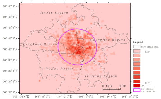
Figure 1.
Point kernel density distribution and direction ellipse.
3.2. Spatio-Temporal Snapshot
We use the spatio-temporal cube (Figure 2a) to model the above trajectory data. The spatio-temporal cube model is a 3D geo-visualization and analysis tool that can perform spatio-temporal data mapping. Data at the same spatial location but different time share the same location ID to form a bar time series; data covering the same time range but different spatial locations share the same time ID to form a time slice. Based on this model, we can describe the data systematically at three levels: semantic, spatial, and temporal. The model performs well in data sharing, storage, and query, which is beneficial to dynamic community segmentation and data spatio-temporal pattern mining [27,28].
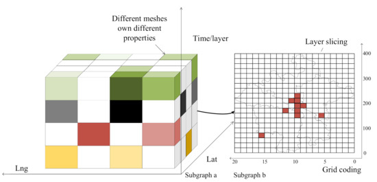
Figure 2.
Space-time cube model (The left side is the a-subfigure, which shows the cube model, and the right side is the b-subfigure, which shows the layer slice).
The study area is divided into regular grids and encoded according to latitude and longitude as shown in Figure 2b. Compared with the subjectively defined macroscopic divisions of areas, such as provincial divisions, regular grids with fine resolution are more objective and more sensitive to details [29].
4. Methods
Figure 3 shows the flowchart of our approach to construct a complex network of traffic flows based on cab trajectories and discusses the interaction and directionality of the network. In addition, we analyze the structure of the city and discuss the key nodes in the city. The paper is divided into the following four parts: data arrangement, time and space properties, small-worlds and scale-free for complex networks, and the discussion. The core algorithm pseudo-code is in Appendix A1.
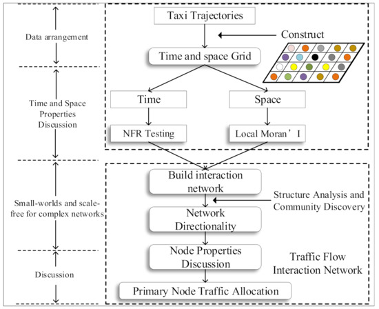
Figure 3.
Method flow chart.
4.1. Complex Network Analysis Framework
Networks are a general language for describing complex systems of interacting entities [30]. Normally, a network (graph) G is mathematically defined as:
where V is the set of all vertices (nodes) and M is the set of all the edges between each pair of nodes. The edges show how nodes are connected, and a weight matrix M is defined to represent the strength of connections.
where m is the number of nodes that have been determined, is the number of orders from data point i to data point j. The larger means the stronger the correlation between regions.
Community structure is an important topological feature of complex networks [18]. A community of a network refers to a set of nodes that share similar features and the interactions among them are more frequent than that with nodes from different communities.
Community structure detection is the process of dividing every node into different communities based on directed connection between nodes in a complex network [31]. Common algorithms for community structure detection include graph segmentation theory [32], Louvain algorithm, GN algorithm, Newman fast algorithm, and other algorithms, which are often utilized in constructing social networks of the social media users and automatic contact recommendation.
The spatial adjacency matrix is a component of spatial modeling, which is defined as an expression of spatial dependence between observations [33].
In reality, there are a large number of residential activities in the OD point aggregation areas of cab trajectories, and these aggregation areas are the spatial hotspots of the city. If there are many trajectories with the same OD points, this implies that there is some spatial correlation between the two areas. Based on this correlation, we build a complex network of traffic flow [34].
The Louvain method is a simple, efficient, and easy-to-implement method for identifying communities in complex networks. The method unveils hierarchies of communities and allows to zoom within communities to discover sub-communities, sub-sub-communities, etc. It is, today, one of the most widely used methods for detecting communities and could take all the edge nodes into consideration and the community structure produced by it is hierarchical [27,35,36]. Evaluation of classification by this algorithm is based on modularity. The greater the modularity degree, the more obvious the community structure. The mathematical definition of modularity degree is:
where is the weight of the edge between node i and node j, is the degree of the node (The number of arc tails of nodes plus the number of arc headers), m is the total number of nodes in a complex network, and is the community with the node i. If , and if , . In the random case, the number of edges between nodes is . The value range of Q is [26,37]. The specific flow of the Louvain algorithm is:
- 1.
- Each node is treated as a separate community, and the numbers of communities and grids (nodes) are the same at the very beginning;
- 2.
- traversal means a node i, consider its neighbor j. Then remove node i from the community that node i belongs to, and then add it to the community that node j belongs to. Later, calculate and compare the changes in modularity and place node i in the community where the modularity degree increases the most. If the node j with positive modularity returns cannot be found, node i shall be maintained in its original community;
- 3.
- repeat step 2. Apply this process to all nodes until the local maximum of modularity is reached, i.e., no node can further increase the network modularity and the community structure will not change any more;
- 4.
- compress the community structure obtained in step 3. The original community is compressed into new nodes, then the weight of nodes within the original community is transformed into the weight of new node ring, and the weight of edge between original communities is transformed into the weight of edge between nodes;
- 5.
- repeat step 1 until the community structure no longer changes.
4.2. Net Flow Ratio Analysis
The net flow ratio (NFR) is the ratio between the net inflow from other regions to a designated region and the total flow from that region in a given time period. The range of this indicator is [−1, 1], which can reflect the relative heat of a region to some extent. When NFR > 0, it means that the attractiveness of the region to the population is increasing, otherwise the attractiveness of the region to the population is decreasing. When NFR = −1, it means that the region has only outflow but not inflow during the study time; when NFR = 1, it means that the region has only inflow but not outflow. The formula for calculating NFR is:
where is the inflow intensity; is the outflow intensity.
4.3. The Analysis of Anselin Local Moran’s I
The criterion for spatial clustering and anomaly detection is based on Anselin Local Moran’s I [38,39]. A positive index of a region indicates the existence of spatial “high-high ” or “low-low” clustering in the region, i.e., spatial elements with similar attribute values are adjacent to each other. A negative value of this index indicates the existence of spatial anomalies when the values of adjacent spatial elements differ significantly. Spatial anomalies are further divided into “high-low” clusters where high values surround low values and “low-high” clusters where low values surround high values. The local Moran index is defined as follows:
Among them:
is the attribute of the element i, is the average value of the corresponding attribute of the element, and represents the spatial weight between the elements. The p-value is the level of significance. For the pattern analysis tools, it is the probability that the observed spatial pattern is created by some random process. When the p-value is very small, it means it is very unlikely (small probability) that the observed spatial pattern is the result of a random process, so you can reject the null hypothesis. z-scores are standard deviations. The z-scores and p-values are measures of statistical significance that tell you whether or not to reject the null hypothesis. In fact, they indicate whether apparent similarity (a spatial clustering of either high or low values) or dissimilarity (a spatial outlier) is more pronounced than one would expect from a random distribution.
We only marked grids with confidence levels greater than 95% (p < 0.05) as clusters or outliers, and other regions were not significant.
5. Results and Findings
This section discusses spatial and temporal analysis, construction, and interaction analysis of urban traffic flow network.
The first analysis discusses hotspot grids and hotspot areas and their associations with residential mobility patterns, land use, accessibility, and the urban functions of different communities. Second, we discussed the community attributes of complex networks. The connections within communities are much greater than those outside of them, and our research shows that residents in different areas have different ranges of daily commuting life, and that work and life needs can be met within communities.
This section also provides two meaningful visualization methods. (1) We can see that the network composed by traffic flow is consistent with the small-world and scale-free characteristics of complex networks. (2) We propose a method to construct an urban direction vector field, which can see more information about the regional direction.
The experiments in this paper used the network computing library in python (Networkx V2.1), as well as Arcgis 10.5 map processing software and GeoDa (V1.18) spatial analysis software.
5.1. Spatial and Temporal Analysis of Traffic Flow
5.1.1. Temporal Characteristic Analysis
The frequency distribution of resident trips during the study period is shown in Figure 4. The most popular travel time was Saturday at 5:00 p.m. (5 November), with 14,901 cab orders occurring in one hour. Orders were higher on Mondays, Fridays, and Saturdays during the study interval, while 1:00 p.m., 2:00 p.m., and 5:00 p.m. are the most active times of the day for urban traffic.
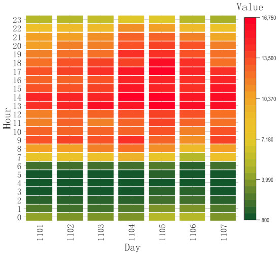
Figure 4.
Thermogram of taxi orders.
5.1.2. Spatial Feature Analysis
According to previous studies, segmenting the study area using regular grids with fine resolution is better than using administrative divisions. The size of grid can affect the result of spatial feature analysis [40,41]. Smaller grids can preserve more urban details. However, a smaller grid is not necessarily better. If the grid is too small, the overall geographic entity may be segmented and the number of cab orders in the grid may be reduced, which increases the risk of unexpected errors. In this paper, the study area is divided into a grid, and the actual side length of the grid is set to about 500–600 m after calculation and comparison.
We counted the number of orders in each grid, as shown in Figure 5A. As we expected, business districts, scenic spots, bus stations, and train stations in the city with high traffic flow are the areas with high density of cab orders. Taxi orders show an irregular concentric circle structure, and the number of orders decays from the city center outward in order, with the largest spatial grid exceeding 2000 orders per day. The grids with more than 900 orders are distributed around important POIs such as Chengdu East Station, Wuhou Temple, and Zhaogeji Bus Station.
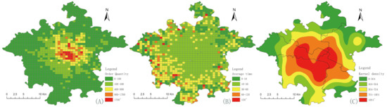
Figure 5.
Thermogram of trip frequency. (Subplot (A) shows the order density distribution, subplot (B) shows the average order length distribution, and subplot (C) shows the public transportation density distribution).
We discuss the order lengths in Figure 5B, which are within half an hour for orders originating in the city center due to more convenient public transportation in the city center, and longer in the southwest of the city than in the northeast. The average order length is more than one hour at passenger stations with more foreign visitors (Chengdu Station and Chengdu East Station) and at scenic spots with less convenient transportation, such as Chengdu Research Base of Giant Panda and Happy Valley. As shown in Figure 5C, the longer the duration of cab orders, the lower the density of bus stops in the area. In other words, taxi order duration is negatively correlated with bus stop density.
5.1.3. Net Flow Ratio
In order to study the inflow and outflow in the study area at different moments, we selected four time periods, i.e., 7:00–9:00 a.m., 12:00–2:00 p.m., 6:00–8:00 p.m., and 9:00–11:00 p.m. for spatio-temporal snapshots, and pre-processed the trajectories of these time periods. The processing rules are as follows:
1. orders less than 10 in the grid during the time period are considered as invalid grids for filtering; 2. according to different NFR, we define 6 types of grids; 3. the study area is divided into spatial scale grids; 4. the traffic flow OD points are all located in the study area.
Figure 6 shows the calculation results of NFR for different areas of the city. During the morning peak hours, the flow of people is directed to the city center as well as to various passenger stations (airport, passenger station, railway station). At night, the city center and passenger stations basically show a net outflow. The northern and eastern parts of the study area have increased attractiveness, presumably these areas have more residential areas.
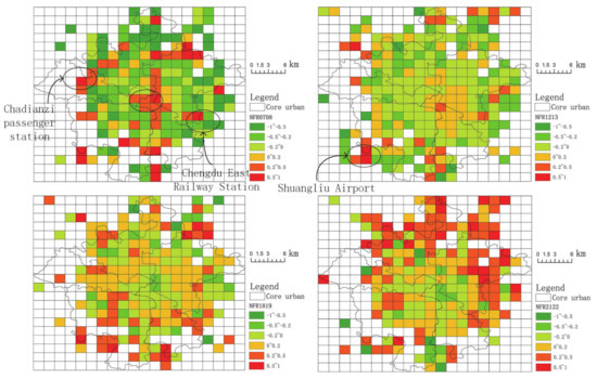
Figure 6.
Distribution of spatial net flow ratio in four time periods. (The four time slots are 7:00–9:00 a.m., 12:00–2:00 p.m., 6:00–8:00 p.m., and 9:00–11:00 p.m.).
5.1.4. Spatial Clustering and Outlier Detection
In addition to the discussion of urban hotspots using NFR metrics under the temporal perspective, we also used spatial statistical methods to detect spatial clustering and anomalies in the study area. As shown in Figure 7, we classified the study area into seven types: H-H Class, H-L Class, L-H Class, L-L Class, insignificant Class (No significant spatial correlation), and insufficient data Class (insufficient data for intra-regional studies). Consistent with the above study, the city center belongs to the “high-H” cluster, indicating that the area is a high volume of cab orders and active commuting area. In addition to this, we detected some very interesting areas. Around the “high-high” clusters, there are “low-high” outliers marked in blue (Figure 7B).
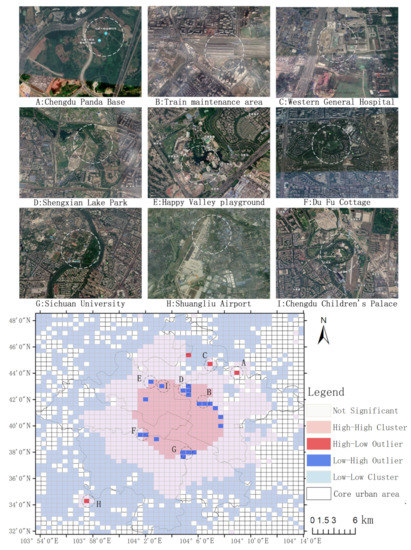
Figure 7.
Spatial clustering and outlier analysis. (The above subplot is the remote sensing image of each clustering area, and the following subplot is the spatial detection result).
We show satellite images of these locations in Figure 7, which are: the Train Maintenance Center (B) and Shengxian Lake Park (D), Du Fu’s Thatched House and the adjacent Huanghuaxi Park (F), Wuhou Temple and the nearby university campus (G), the Children’s Palace (I), and the sports center and amusement park. These areas have distinct recreational and tourism attributes.
Correspondingly, the “low-low” agglomerations are mixed with “high-low” (marked in red) spatially anomalous areas that have far more cab orders than the surrounding areas. These areas are: Panda Base (A), Large Hospital (C), Airport (H), and Logistics Center. The appearance of spatial anomalies is closely related to the urban functions of the spatial grid.
5.2. Construction and Interaction Analysis of Urban Traffic Flow Network
5.2.1. Urban Community Structure and Flow Direction
Networks composed of traffic flows are a type of complex networks that possess small-world and scale-free characteristics. The scale-free feature of complex networks means that most of the nodes in the network are connected to very few nodes, while very few nodes are connected to a very large number of nodes. The presence of such critical nodes (called “hubs” or “hub-and-spoke nodes”) makes scale-free networks robust to unexpected failures, but vulnerable to coordinated attacks. The small-world feature refers to the fact that most of the nodes in the network are not connected to each other, but most of them are reachable in a few steps.
Community structure is one of the important characteristics of urban traffic flow networks. We use spontaneously generated trajectory data (Volunteered Geographic Information data) covering a wide range of cities to parse the urban structure [42,43].
We use the following metrics for our evaluation:
- Degree of node: the size of traffic flow leaving the node and the size of traffic flow entering the node, node degree = out degree + in degree. As shown in Figure 8, the size of the node represents the degree of the node.
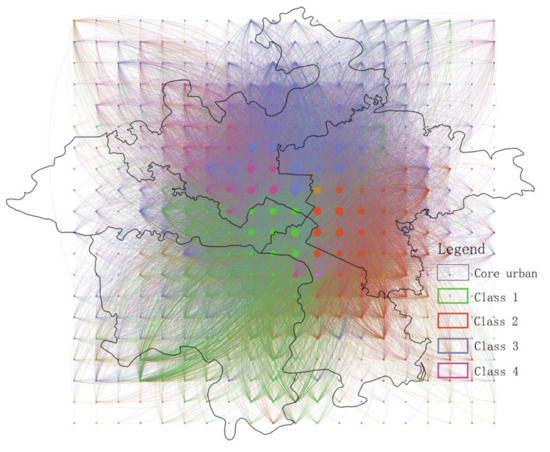 Figure 8. Community structure and small world characteristics of traffic flow network. (The graph density is 0.115, the average degree is 45.788, and the average weighted degree is 513.745; class is also referred to as community in this article).
 - Average degree: the weighted average of all node degrees.
- Network diameter: the maximum value of the shortest distance between any two points in a complex network. The smaller the metric represents the higher the degree of communication.
- Graph Density: the higher the graph density, the more complex the network and the tighter the internal connections.
- Modularity Degree: the larger the value, the more pronounced the community structure.
- Cluster coefficient: the clustering coefficient (also known as clustering coefficient, clustering coefficient) is the coefficient used to describe the degree of clustering between the vertices of a graph. Specifically, it is the degree to which the adjacent points of a point. For example, the degree to which your friends know each other on social networks in life [43].
- Betweenness centrality is an indicator of a node’s centrality in a network. It is equal to the number of shortest paths from all vertices to all others that pass through that node. A node with high betweenness centrality has a large influence on the transfer of items through the network, under the assumption that item transfer follows the shortest paths.
- Closeness centrality of a node is a measure of centrality in a network, calculated as the reciprocal of the sum of the length of the shortest paths between the node and all other nodes in the graph. Thus, the more central a node is, the closer it is to all other nodes.
The study area was divided into 400 grids (points) with a total of 18,315 connected edges between these grids. As shown in Figure 8, our traffic flow network clustering coefficient is 0.765, and the study area is divided into 13 communities with an overall network modularity of 0.124. The four largest communities cover 37.75%, 22.25%, 16.75%, and 11.25% of the area, respectively. The boundaries between communities are influenced by the main urban traffic arteries. The diameter of the network is 4, the average path length is 1.944, and the distance between any two locations is no more than two grids, reflecting a strong small-world characteristic (Shorter average path length and larger clustering coefficients)[44].
The community detection method has proven to be an effective tool in urban planning [45]. The impact of railroads and trunk roads on community boundaries is more pronounced than that of administrative boundaries. In addition, we calculate the weighted average of azimuth angles between OD points in different areas and construct direction vector field to represent the directionality of different locations. As shown in Figure 9, the arrows indicate the OD direction of each grid.
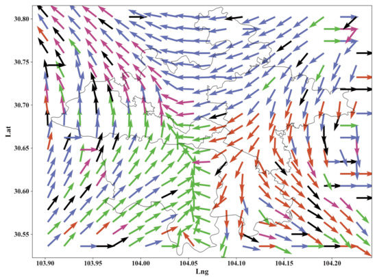
Figure 9.
Traffic flow network direction vector field and scale-free characteristics. (Arrows represent the Origin-Destination (OD) direction of different grids, arrows of different colors represent different communities, the largest four communities are represented with the same colors as Figure 8, and the rest of the communities are represented in black).
In Green Community 1, there is a very interesting region (104.05 E, 30.55–30.65 N). The nodes in the two sides of this area are in opposite directions, and the nodes in the middle area point to the urban area; this area belongs to the urban axis of Chengdu. The node direction of Community 1 points to the city center, while the nodes of Community 2 and Community 4 point to the direction out of the city. The grid direction of Community 3 is more complex, and the trajectory is concentrated in the north area of the city.
5.2.2. Urban Community Structure and Flow Direction
We discuss all 400 grid attributes, with the horizontal axis representing the node IDs and the vertical axis representing the degrees of the nodes, and the results are listed in Figure 10 and Table 1.
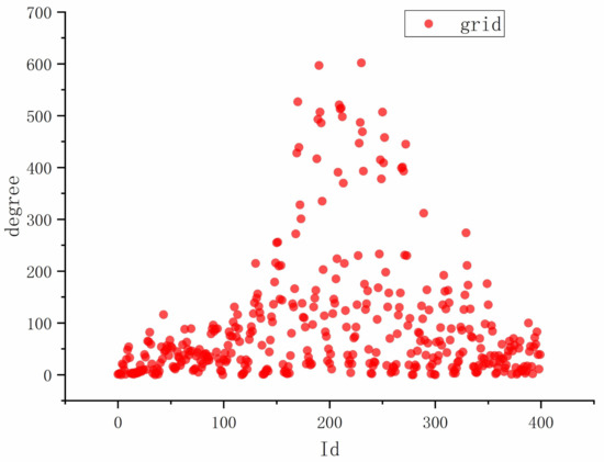
Figure 10.
Network node degree display. (The location degree values are higher for node IDs around 200 near the city center, which is consistent with the results of Figure 8, where the nodes in the city center have the most traffic and show scale-free characteristics).

Table 1.
Calculation results of complex network node.
As shown in Table 1, we list some nodes with high degree values. The betweenness centrality of nodes is an indicator that controls the interaction ability of urban traffic flow network, i.e., the traffic transit or interchange ability of a certain area in the city, and these nodes are often surrounded by areas with more intensive economic activities and play the role of traffic hubs in the whole city. Nodes with high betweenness centrality have considerable influence in the urban traffic flow network because they control the information transfer between other nodes. At the same time, these nodes are also the most vulnerable nodes, and disturbances to these nodes can disrupt the interactive links between other nodes.
The closeness centrality is measured from the whole network, the ability of a node not to be influenced by the rest of the nodes, and is more concerned with the shortest path directly between two regions. If a node can establish a connection with the rest of the nodes through a shorter path with the help of a small number of nodes, it means that this node has a higher independence, and thus a higher closeness centrality.
In addition, we also count the number of trajectories with these nodes as the origin (origin points, count_o) and the total order time (time_sum), the number of trajectories with these nodes as the destination (destination points, count_d), as well as the latitude and longitude values of these nodes and the communities they belong to.
We constructed a new local network from these key nodes and examined the traffic flow between them. The width of the edges is shown proportionally to the traffic flow; the wider the edge, the larger the value. As can be seen from the Sankey diagram in Figure 11, the grid node with ID 190 receives the most traffic flow, showing the scale-free characteristics of the local network (a small number of nodes enjoy most of the traffic).
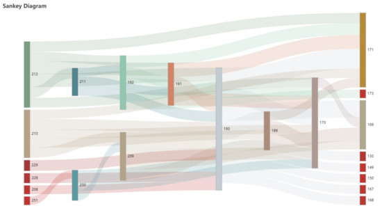
Figure 11.
Scale-free characteristics and flow analysis of fine particle network.
5.2.3. Community Indicators
Graph density measures the strength of internal associations between modular classes in a network, and a high value means that the community has a higher density of spatial nodes and more frequent internal connections. Centrality to measure the local traffic frequency of the network. Comparing the attributes of these four communities, it can be seen from Figure 12 that the density of communities 1, 2, and 4 is higher than the average density of the entire network (0.115). The detailed attributes of these communities are presented in Table 2. In general, the attributes of the four communities are significantly different from each other, and the correlation between the communities is not high.
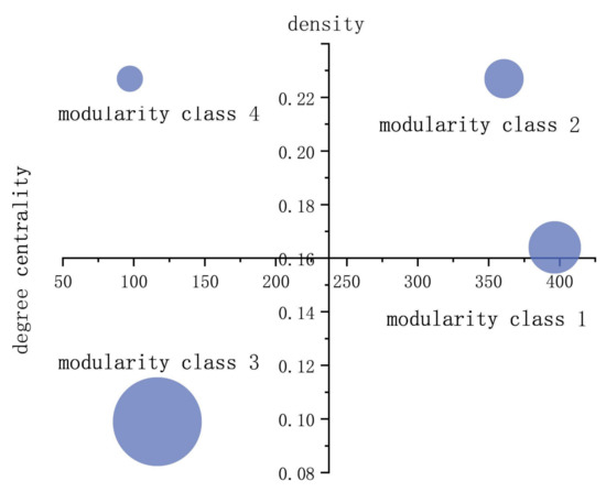
Figure 12.
Attribute comparison of four modularity communities in traffic network.
Table 2.
Calculation results of community attributes of complex networks.
Modularity class 1 has a moderate density, but the nodes have the highest average importance, which indicates that these nodes have a high traffic flow and extensive coverage (southwest part of the city). Modularity class 2 has a high centrality and density, indicating that the area is busy and the nodes are all relatively important. Modularity class 3, the community with the most nodes, has the lowest graph density and low centrality, indicating that the traffic flow distribution in this area is more dispersed. Modularity class 4 has a relatively high graph density and the lowest centrality, which indicates that the nodes are more closely connected to each other, but not the core communities with high traffic flow.
6. Research Conclusions and Discussion
In this paper, a spatio-temporal cube model based on fine-grained spatial grid was introduced, we explored the spatial and temporal correlation of urban hot spots and detected urban structure using the taxi trajectory data. We divided the five core administrative regions of Chengdu into a 50-by-50 grid, and respectively discussed the tine-distribution characteristics, spatial-distribution characteristics and average-length-distribution characteristics of taxi orders. We conducted spatial hotspot mining on the data of 200,000 taxi orders, searched for active and representatively important areas in the city, and then mined the community structure according to the spatial grid. We discussed the correlation between the estimation results of bus stop core density and taxi trip data, and then used the spatial hotspot discovery algorithm to explore the hot grid of different times in the city and to constructs the complex urban traffic network. Compared with representing network nodes with administrative divisions, the spatial grid based on fine particles can avoid the tracks being torn apart, and help to excavate more representative nodes in urban areas.
The results show that the peak hours of taxi trips are 13:00, 14:00, and 17:00, and that residents are more active at noon and after work. The order density basically presents a concentric circle structure, which decreases as the distance from the city center increases. The locations where passenger call for a taxi spread along the main road to the suburbs. Orders in urban areas are generally short-distance trips within half an hour. The order duration is higher in southwestern Chengdu and lower in northeastern Chengdu, which is inversely proportional to the density of bus stations. The results of clustering show that most of the orders come from the area within the third ring line and the density in the second ring line is much higher than that in the surrounding area. The urban traffic network conforms to the characteristics of complex network, and presents obvious community structure. Modularity class 2 has high centrality and density. We divided 400 grids into 6 communities by the fine-grained grid method so that the characteristics of the complex network are verified and the tidal effect of urban population as well as the attraction of residential areas to population at night are found with the net flow ratio.
The data sampled for our study are narrow (7 days) and ignore the seasonality of months. Future work will enhance the generalizability of the model. Enables models to automate/standardize calculations and compare differences in trends in urban structure over time series.
Author Contributions
Methodology, Yan Zhang.; Writing—original draft, Yan Zhang; Visualization, Yan Zhang and Xiang Zheng; Writing—review & editing, Min Chen and Yingxue Yan; Funding acquisition, Yingbing Li; Investigation, Peiying Wang and Yingbing Li. All authors have read and agreed to the published version of the manuscript.
Funding
This work was supported by the National Key Research and Development Program of China under Grant 2018YFC0807000.
Data Availability Statement
The dataset used in this paper is provided by Drip (Gaia Data Development Program) and can be requested for scientific use at the following link at https://outreach.didichuxing.com/research/opendata (accessed on 30 March 2021).
Acknowledgments
The numerical calculations in this paper have been done on the supercomputing system in the Supercomputing Center of Wuhan University. Our deepest gratitude goes to the anonymous reviewers for their careful work and thoughtful suggestions that have helped improve this paper substantially.
Conflicts of Interest
The authors declare no conflict of interest.
Appendix A. Core Algorithm Pseudocode
| Algorithm 1: Traffic flow interaction analysis framework. |
 |
References
- Zhang, S.; Tang, J.; Wang, H.; Wang, Y.; An, S. Revealing intra-urban travel patterns and service ranges from taxi trajectories. J. Transp. Geogr. 2017, 61, 72–86. [Google Scholar] [CrossRef]
- Yang, Z.; Franz, M.L.; Zhu, S.; Mahmoudi, J.; Nasri, A.; Zhang, L. Analysis of Washington, DC taxi demand using GPS and land-use data. J. Transp. Geogr. 2018, 66, 35–44. [Google Scholar] [CrossRef]
- Zhang, A.; Xia, C.; Chu, J.; Lin, J.; Li, W.; Wu, J. Portraying urban landscape: A quantitative analysis system applied in fifteen metropolises in China. Sustain. Cities Soc. 2019, 46, 101396. [Google Scholar] [CrossRef]
- Zambrano-Martinez, J.L.; Calafate, C.T.; Soler, D.; Cano, J.C.; Manzoni, P. Modeling and characterization of traffic flows in urban environments. Sensors 2018, 18, 2020. [Google Scholar] [CrossRef]
- Weyns, D.; Holvoet, T.; Helleboogh, A. Anticipatory vehicle routing using delegate multi-agent systems. In Proceedings of the 2007 IEEE Intelligent Transportation Systems Conference, Bellevue, WA, USA, 30 September–3 October 2007; pp. 87–93. [Google Scholar]
- Fouladgar, M.; Parchami, M.; Elmasri, R.; Ghaderi, A. Scalable deep traffic flow neural networks for urban traffic congestion prediction. In Proceedings of the 2017 International Joint Conference on Neural Networks (IJCNN), Anchorage, AK, USA, 14–19 May 2017; pp. 2251–2258. [Google Scholar]
- Mackenzie, J.; Roddick, J.F.; Zito, R. An evaluation of HTM and LSTM for short-term arterial traffic flow prediction. IEEE Trans. Intell. Transp. Syst. 2018, 20, 1847–1857. [Google Scholar] [CrossRef]
- Alfeo, A.L.; Cimino, M.G.C.A.; Egidi, S.; Lepri, B.; Vaglini, G. A stigmergy-based analysis of city hotspots to discover trends and anomalies in urban transportation usage. IEEE Trans. Intell. Transp. Syst. 2018, 19, 2258–2267. [Google Scholar] [CrossRef]
- Huang, S.S.; Song, R.; Tao, Y. Behavior of urban residents travel mode choosing and influencing factors: Taking Beijing as an example. Commun. Stand. 2008, 9, 1–5. [Google Scholar]
- Liu, J.; Han, K.; Chen, X.M.; Ong, G.P. Spatial-temporal inference of urban traffic emissions based on taxi trajectories and multi-source urban data. Transp. Res. Part C Emerg. Technol. 2019, 106, 145–165. [Google Scholar] [CrossRef]
- Zhao, P.; Kwan, M.P.; Qin, K. Uncovering the spatiotemporal patterns of CO2 emissions by taxis based on Individuals’ daily travel. J. Transp. Geogr. 2017, 62, 122–135. [Google Scholar] [CrossRef]
- Chen, Z.; Yang, Y.; Huang, L.; Wang, E.; Li, D. Discovering Urban Traffic Congestion Propagation Patterns With Taxi Trajectory Data. IEEE Access 2018, 6, 69481–69491. [Google Scholar] [CrossRef]
- Chen, S.; Tao, H.; Li, X.; Zhuo, L. Detecting urban commercial patterns using a latent semantic information model: A case study of spatial-temporal evolution in Guangzhou, China. PLoS ONE 2018, 13, e0202162. [Google Scholar] [CrossRef]
- Tsekeris, T.; Geroliminis, N. City size, network structure and traffic congestion. J. Urban Econ. 2013, 76, 1–14. [Google Scholar] [CrossRef]
- Zhao, X.; Zhang, Y.; Liu, H.; Wang, S.; Qian, Z.; Hu, Y.; Yin, B. Detecting Pickpocketing Gangs on Buses with Smart Card Data. IEEE Intell. Transp. Syst. Mag. 2019, 11, 181–199. [Google Scholar] [CrossRef]
- Zhang, L.; Lu, J.; Zhou, J.; Zhu, J.; Li, Y.; Wan, Q. Complexities’ day-to-day dynamic evolution analysis and prediction for a Didi taxi trip network based on complex network theory. Mod. Phys. Lett. B 2018, 32, 1850062. [Google Scholar] [CrossRef]
- Hincks, S.; Kingston, R.; Webb, B.; Wong, C. A new geodemographic classification of commuting flows for England and Wales. Int. J. Geogr. Inf. Sci. 2018, 32, 663–684. [Google Scholar] [CrossRef]
- Chang, H.w.; Tai, Y.c.; Hsu, J.Y.j. Context-aware taxi demand hotspots prediction. Int. J. Bus. Intell. Data Min. 2010, 5, 3–18. [Google Scholar] [CrossRef]
- Cai, J.; Huang, B.; Song, Y. Using multi-source geospatial big data to identify the structure of polycentric cities. Remote Sens. Environ. 2017, 202, 210–221. [Google Scholar] [CrossRef]
- Tang, J.; Liu, F.; Wang, Y.; Wang, H. Uncovering urban human mobility from large scale taxi GPS data. Phys. A Stat. Mech. Appl. 2015, 438, 140–153. [Google Scholar] [CrossRef]
- Yang, J.; Yi, D.; Liu, J.; Liu, Y.; Zhang, J. Spatiotemporal Change Characteristics of Nodes’ Heterogeneity in the Directed and Weighted Spatial Interaction Networks: Case Study within the Sixth Ring Road of Beijing, China. Sustainability 2019, 11, 6359. [Google Scholar] [CrossRef]
- Zhao, S.; Zhao, P.; Cui, Y. A network centrality measure framework for analyzing urban traffic flow: A case study of Wuhan, China. Phys. A Stat. Mech. Appl. 2017, 478, 143–157. [Google Scholar] [CrossRef]
- Hamedmoghadam-Rafati, H.; Steponavice, I.; Ramezani, M.; Saberi, M. A complex network analysis of macroscopic structure of taxi trips. IFAC PapersOnLine 2017, 50, 9432–9437. [Google Scholar] [CrossRef]
- Kutela, B.; Novat, N.; Langa, N. Exploring geographical distribution of transportation research themes related to COVID-19 using text network approach. Sustain. Cities Soc. 2021, 67, 102729. [Google Scholar] [CrossRef]
- Xu, R.; Yang, G.; Qu, Z.; Chen, Y.; Liu, J.; Shang, L.; Liu, S.; Ge, Y.; Chang, J. City components–area relationship and diversity pattern: Towards a better understanding of urban structure. Sustain. Cities Soc. 2020, 60, 102272. [Google Scholar] [CrossRef]
- Li, L.; Yang, L.; Zhu, H.; Dai, R. Explorative analysis of Wuhan intra-urban human mobility using social media check-in data. PLoS ONE 2015, 10, e0135286. [Google Scholar] [CrossRef]
- Chuangchang, P.; Thinnukool, O.; Tongkumchum, P. Modelling urban growth over time using grid-digitized method with variance inflation factors applied to spatial correlation. Arab. J. Geosci. 2016, 9, 342. [Google Scholar] [CrossRef]
- Li, J.; Chen, S.; Chen, W.; Andrienko, G.; Andrienko, N. Semantics-space-time cube. a conceptual framework for systematic analysis of texts in space and time. IEEE Trans. Vis. Comput. Graph. 2018, 26, 1789–1806. [Google Scholar] [CrossRef]
- Langran, G. A review of temporal database research and its use in GIS applications. Int. J. Geogr. Inf. Syst. 1989, 3, 215–232. [Google Scholar] [CrossRef]
- Leskovec, J.; Kleinberg, J.; Faloutsos, C. Graph evolution: Densification and shrinking diameters. ACM Trans. Knowl. Discov. Data (TKDD) 2007, 1, 2-es. [Google Scholar] [CrossRef]
- Girvan, M.; Newman, M.E.J. Community structure in social and biological networks. Proc. Natl. Acad. Sci. USA 2002, 99, 7821–7826. [Google Scholar] [CrossRef]
- Zhao, P.; Liu, X.; Shen, J.; Chen, M. A network distance and graph-partitioning-based clustering method for improving the accuracy of urban hotspot detection. Geocarto Int. 2019, 34, 293–315. [Google Scholar] [CrossRef]
- Anselin, L.; Lozano-Gracia, N. Spatial hedonic models. In Palgrave Handbook of Econometrics; Springer: Berlin/Heidelberg, Germany, 2009; pp. 1213–1250. [Google Scholar]
- Guo, X.l.; Lu, Z.M. Urban road network and taxi network modeling based on complex network theory. J. Inf. Hiding Multimed. Signal Process. 2016, 7, 558–568. [Google Scholar]
- Gach, O.; Hao, J.K. Improving the Louvain algorithm for community detection with modularity maximization. In Proceedings of the International Conference on Artificial Evolution (Evolution Artificielle), Bordeaux, France, 21–23 October 2013; Springer: Berlin/Heidelberg, Germany, 2013; pp. 145–156. [Google Scholar]
- Zhang, Y.; Chen, N.; Du, W.; Yao, S.; Zheng, X. A New Geo-Propagation Model of Event Evolution Chain Based on Public Opinion and Epidemic Coupling. Int. J. Environ. Res. Public Health 2020, 17, 9235. [Google Scholar] [CrossRef] [PubMed]
- Clauset, A.; Newman, M.E.J.; Moore, C. Finding community structure in very large networks. Phys. Rev. E 2004, 70, 066111. [Google Scholar] [CrossRef]
- Anselin, L. Local indicators of spatial association—LISA. Geogr. Anal. 1995, 27, 93–115. [Google Scholar] [CrossRef]
- Anselin, L. The Moran scatterplot as an ESDA tool to assess local instability in spatial. Spat. Anal. 1996, 4, 111. [Google Scholar]
- Ord, J.K.; Getis, A. Local spatial autocorrelation statistics: Distributional issues and an application. Geogr. Anal. 1995, 27, 286–306. [Google Scholar] [CrossRef]
- Peng, C.; Jin, X.; Wong, K.C.; Shi, M.; Liò, P. Collective human mobility pattern from taxi trips in urban area. PLoS ONE 2012, 7, e34487. [Google Scholar]
- Bastian, M.; Heymann, S.; Jacomy, M. Gephi: An open source software for exploring and manipulating networks. In Proceedings of the International AAAI Conference on Web and Social Media, San Jose, CA, USA, 18–20 May 2009. [Google Scholar]
- Doreian, P.; Lloyd, P.; Mrvar, A. Partitioning large signed two-mode networks: Problems and prospects. Soc. Netw. 2013, 35, 178–203. [Google Scholar] [CrossRef]
- Rüdiger, S.; Plietzsch, A.; Sagués, F.; Sokolov, I.M.; Kurths, J. Epidemics with mutating infectivity on small-world networks. Sci. Rep. 2020, 10, 1–11. [Google Scholar] [CrossRef] [PubMed]
- De Montis, A.; Caschili, S.; Chessa, A. Commuter networks and community detection: A method for planning sub regional areas. Eur. Phys. J. Spec. Top. 2013, 215, 75–91. [Google Scholar] [CrossRef]


Publisher’s Note: MDPI stays neutral with regard to jurisdictional claims in published maps and institutional affiliations. |
© 2021 by the authors. Licensee MDPI, Basel, Switzerland. This article is an open access article distributed under the terms and conditions of the Creative Commons Attribution (CC BY) license (https://creativecommons.org/licenses/by/4.0/).