
A Comparison Method for 3D Laser Point Clouds in Displacement Change Detection for Arch Dams


Abstract
1. Introduction
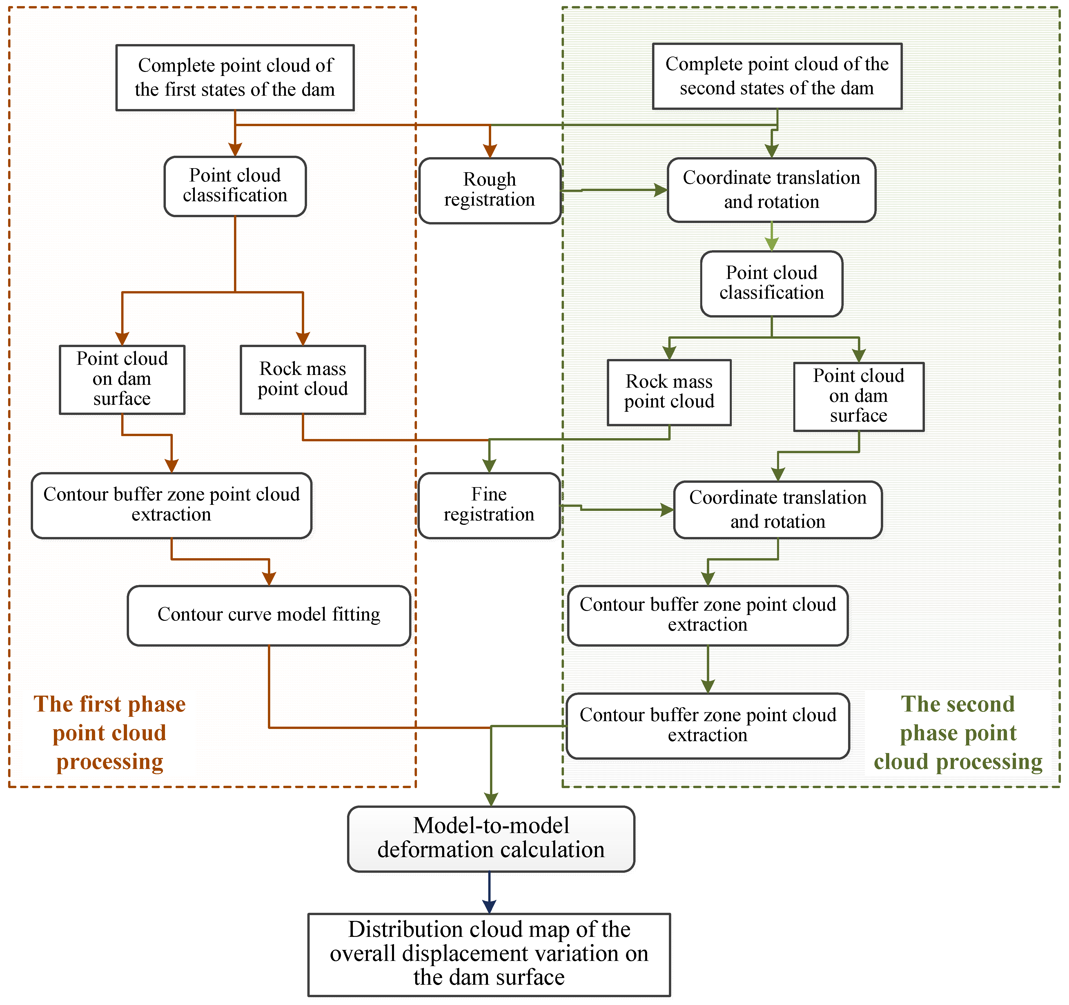
2. Methodology
2.1. Registration
2.1.1. Rough Registration
2.1.2. Fine Registration
2.2. Methods of Point Cloud Comparison
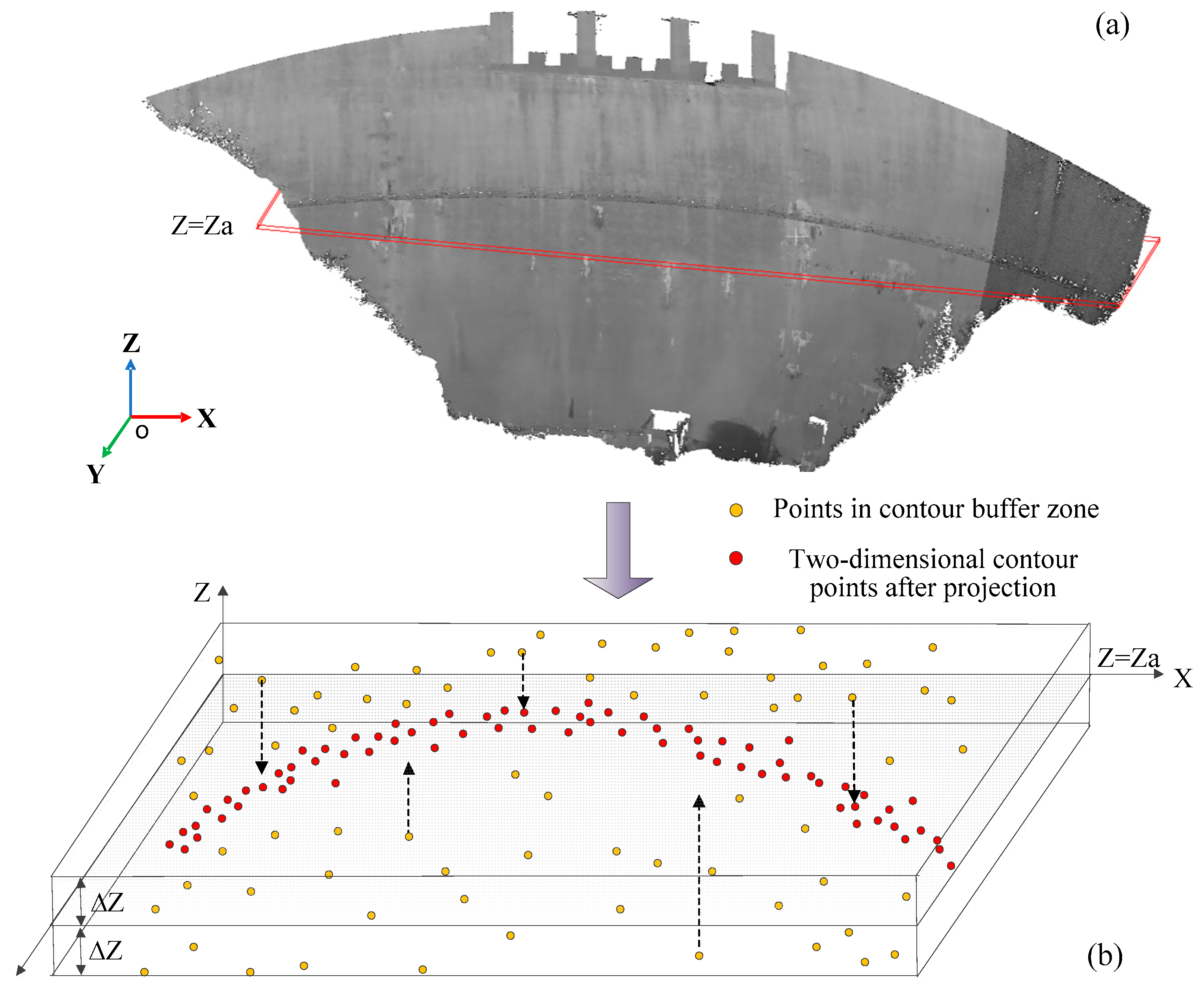
2.2.1. Construction of Contour Model
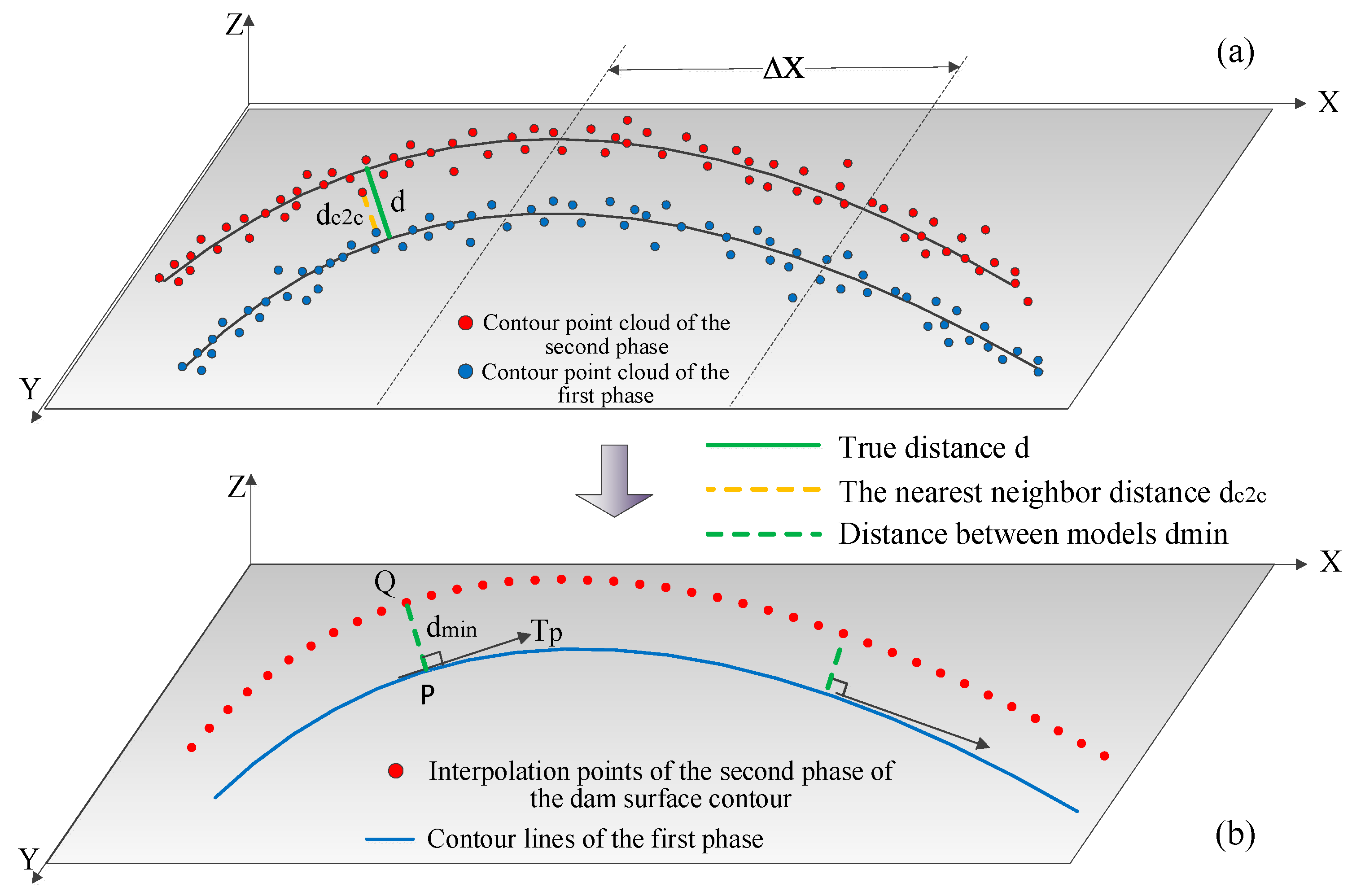
2.2.2. Dam Displacement Variation
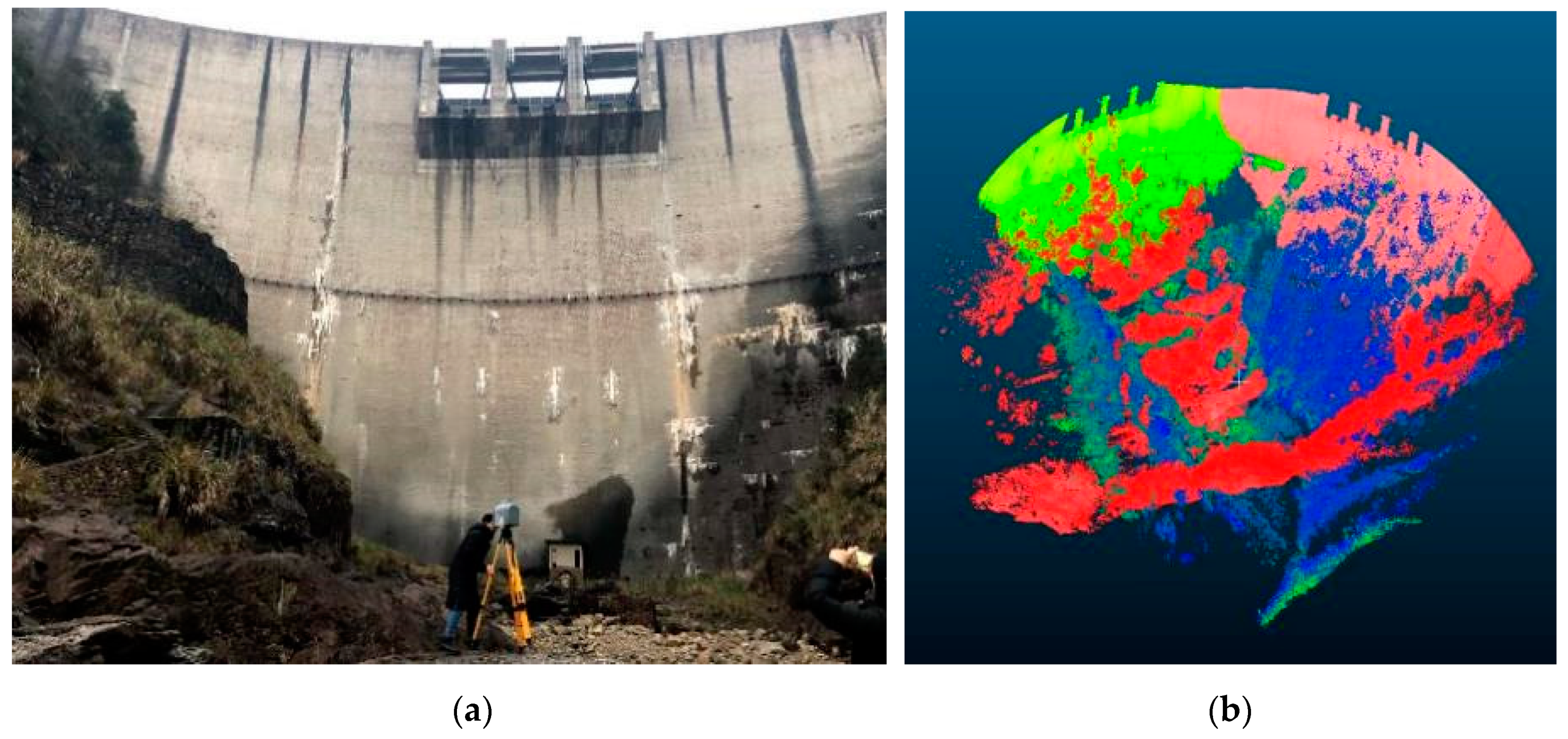
3. Materials
4. Results
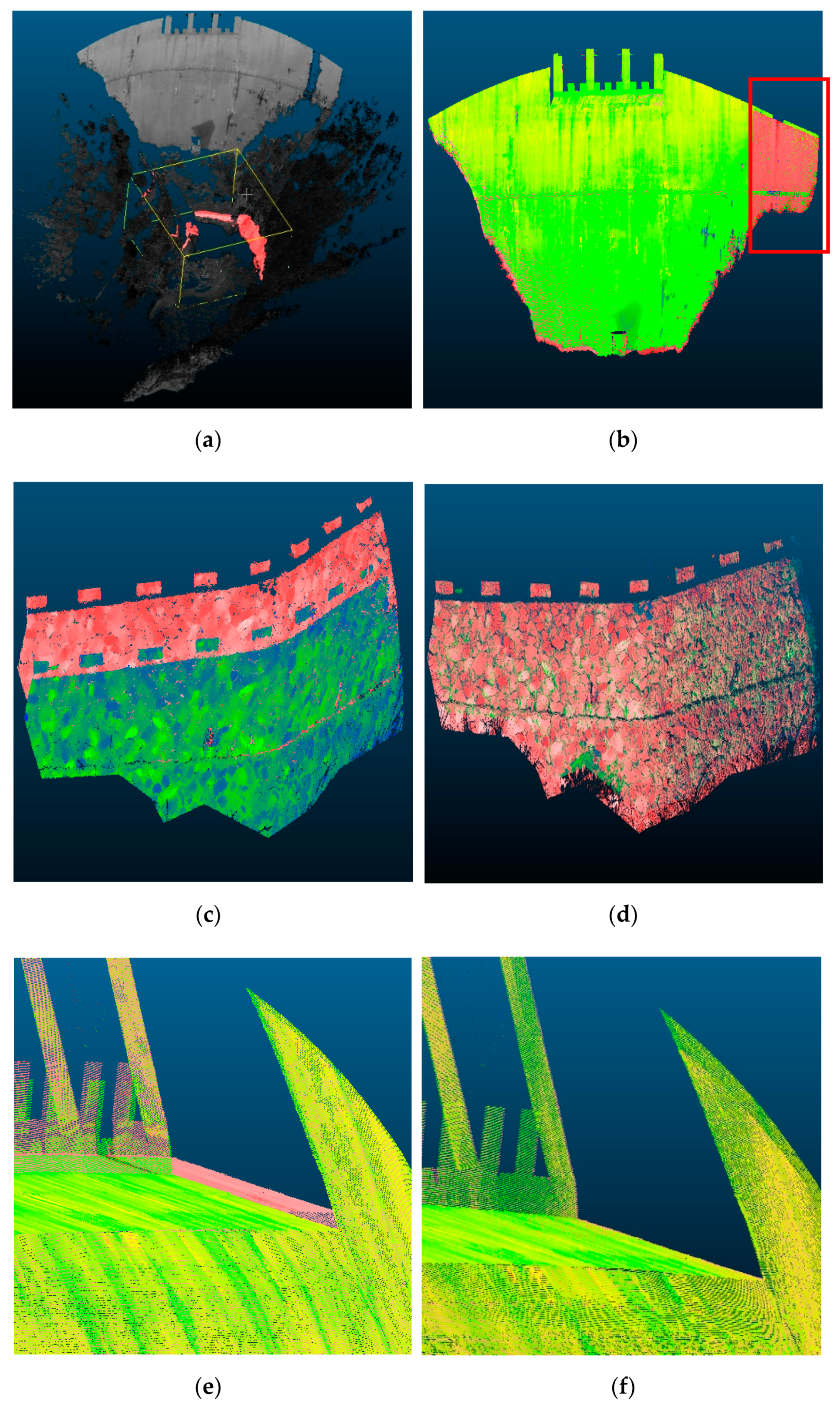
4.1. Two-Phase Point Cloud Registration
4.2. Analysis of Displacement Change
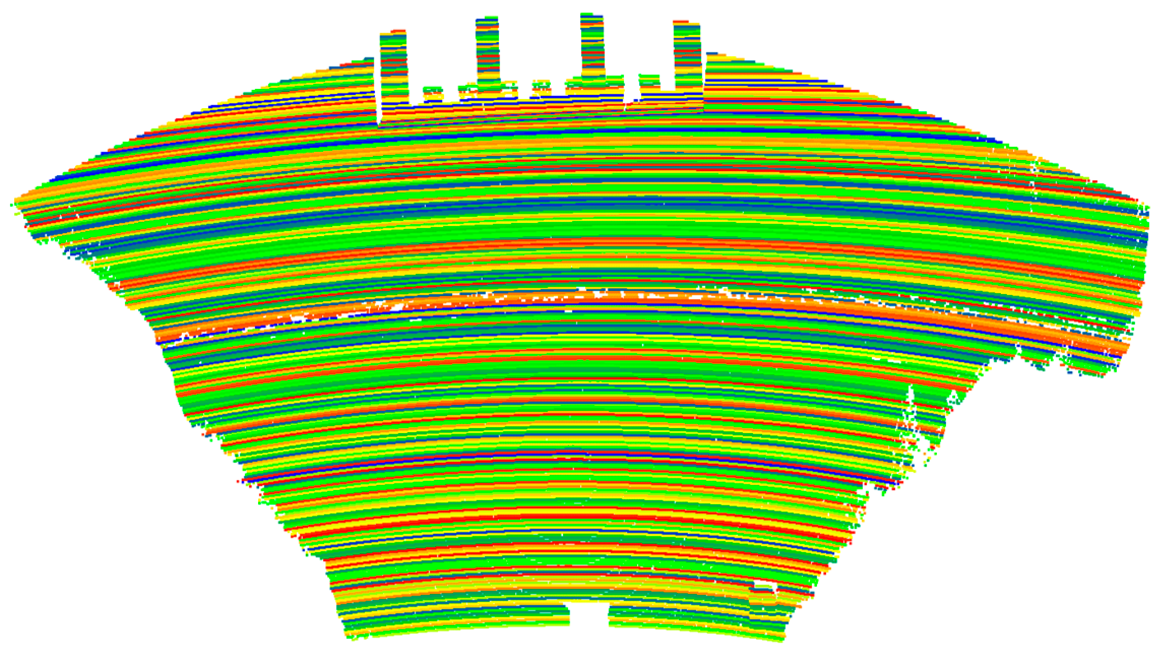
4.2.1. Contour Model Construction and Comparison
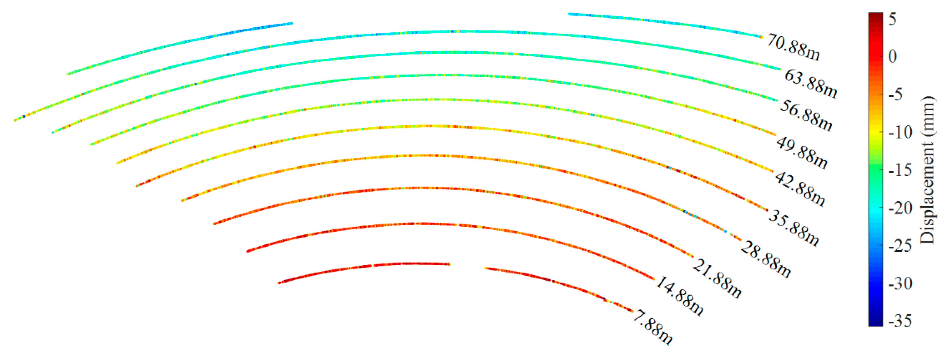
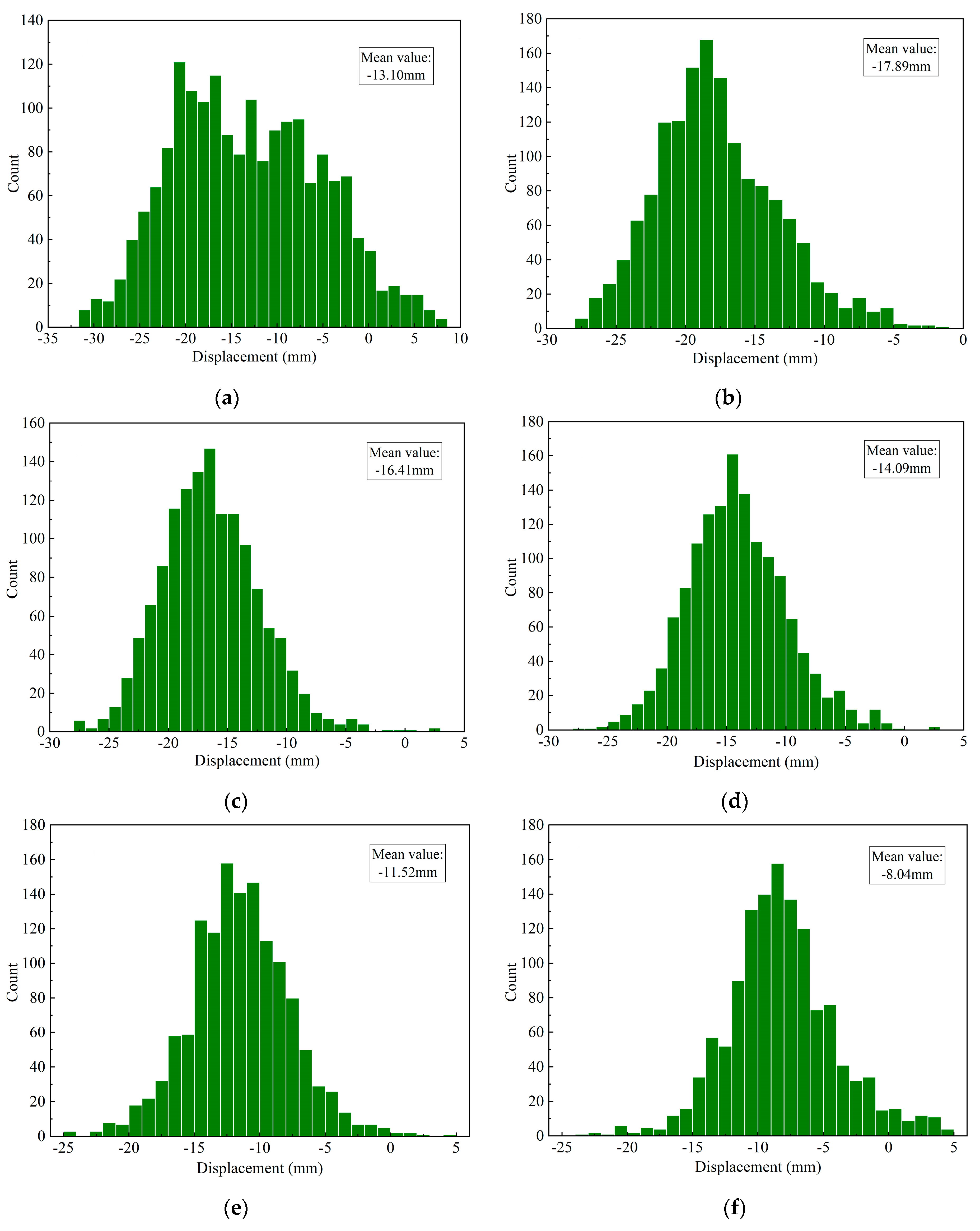
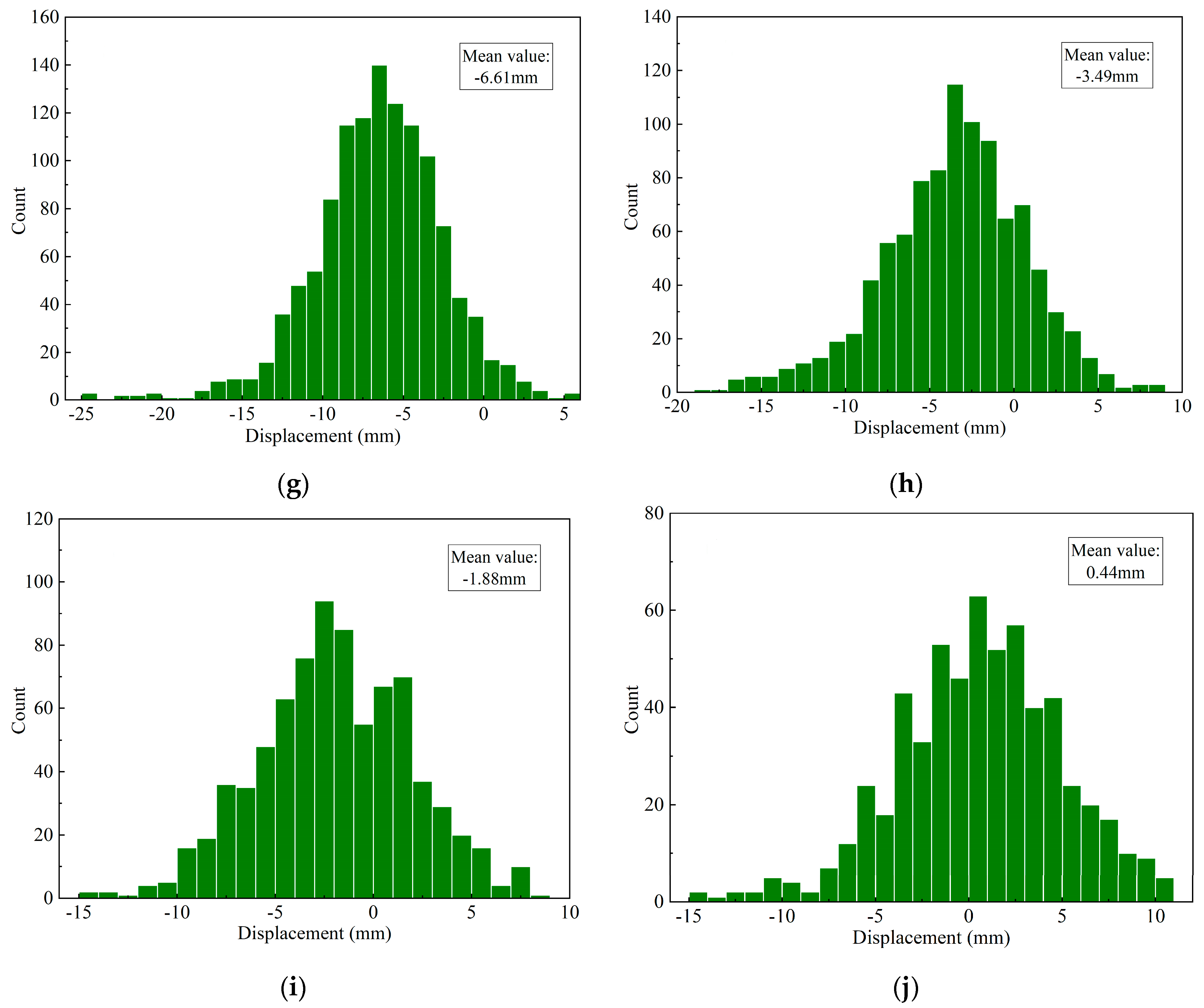
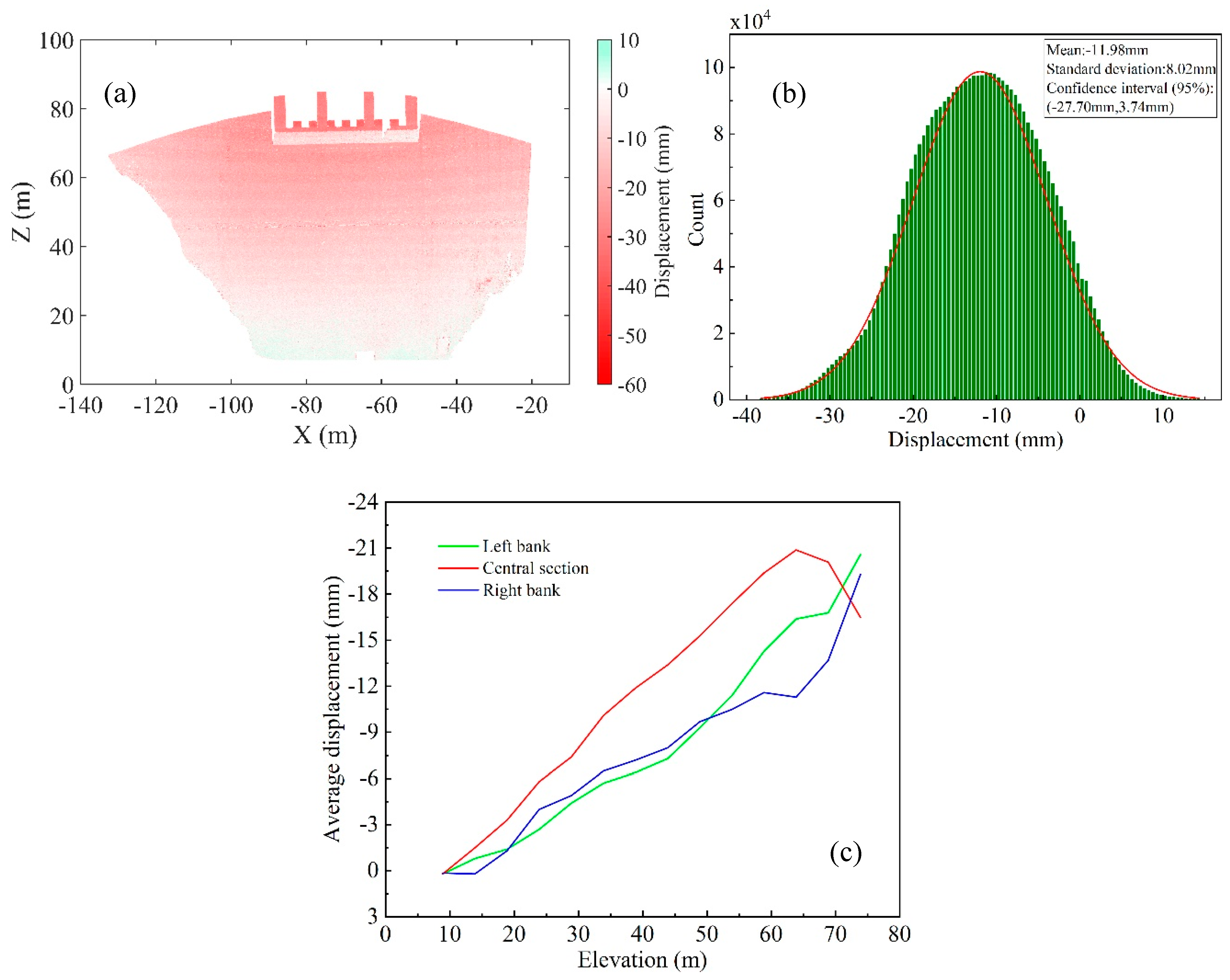
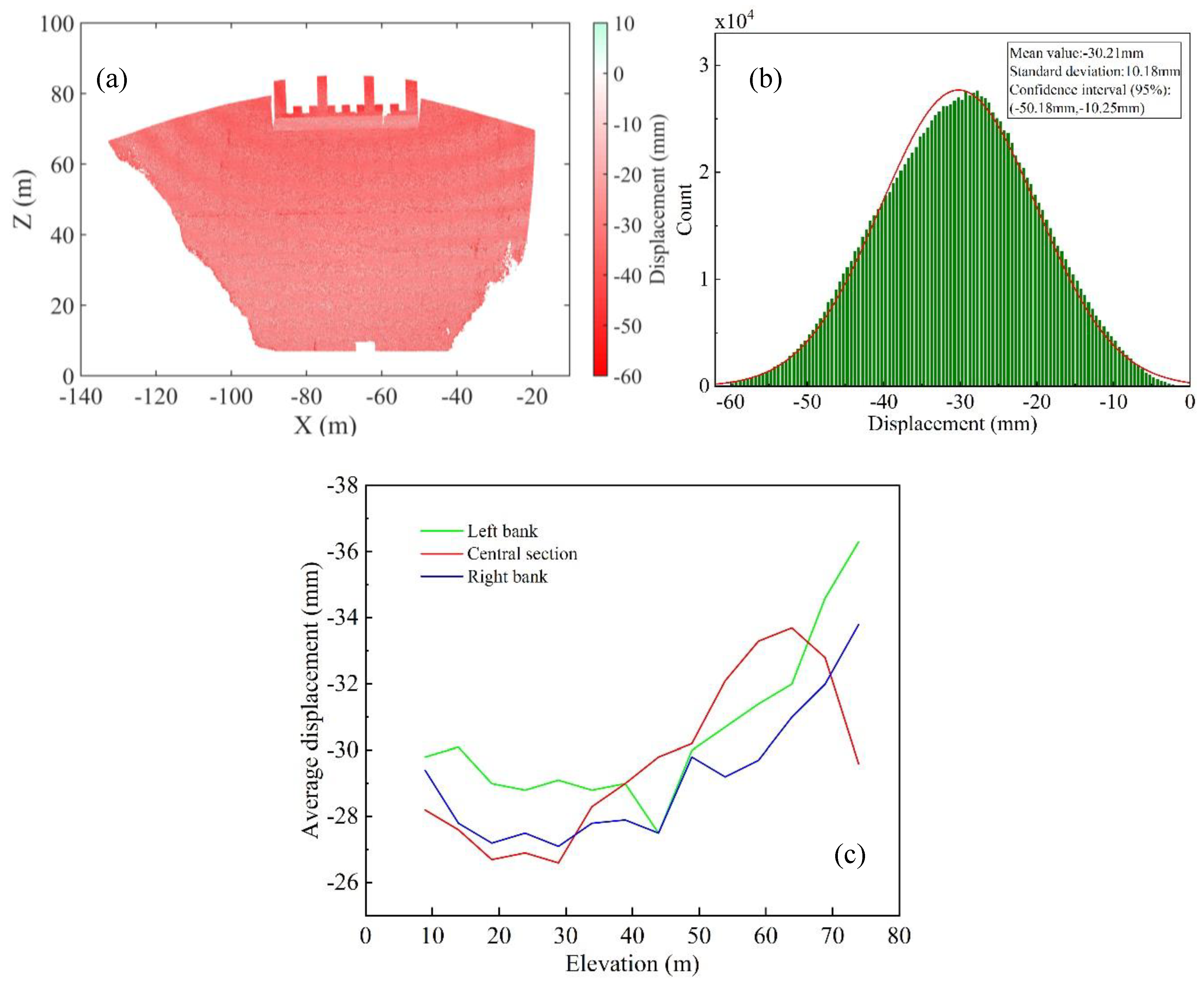
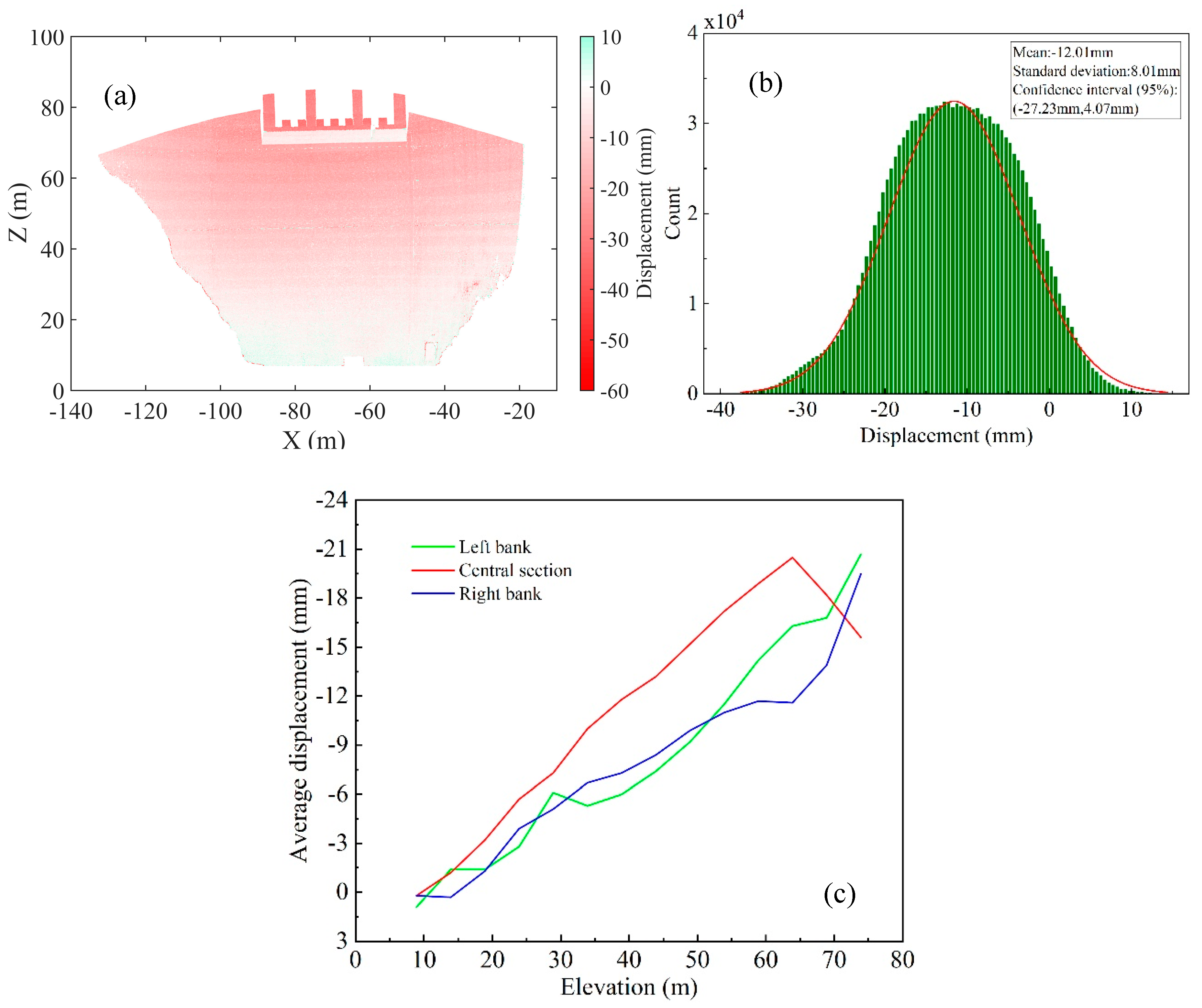
4.2.2. Analysis of Dam Surface Displacement Variation
5. Discussion
6. Conclusions
Author Contributions
Funding
Data Availability Statement
Acknowledgments
Conflicts of Interest
References
- Reyes-Carmona, C.; Barra, A.; Galve, J.P.; Monserrat, O.; Pérez-Peña, J.V.; Mateos, R.M.; Notti, D.; Ruano, P.; Millares, A.; López-Vinielles, J. Sentinel-1 Dinsar for monitoring active landslides in critical infrastructures: The case of the rules reservoir (Southern Spain). Remote Sens. 2020, 12, 809. [Google Scholar] [CrossRef]
- Hamzic, A.; Avdagic, Z.; Besic, I. Multistage cascade predictor of structural elements movement in the deformation analysis of large objects based on time series influencing factors. ISPRS Int. J. Geo-Inf. 2020, 9, 47. [Google Scholar] [CrossRef]
- Li, Y.; Huang, J.; Jiang, S.-H.; Huang, F.; Chang, Z. A web-based gps system for displacement monitoring and failure mechanism analysis of reservoir landslide. Sci. Rep. 2017, 7, 17171. [Google Scholar] [CrossRef] [PubMed]
- Huang, F.; Wu, P.; Ziggah, Y. Gps monitoring landslide deformation signal processing using time-series model. Int. J. Signal Process. Image Process. Pattern Recognit. 2016, 9, 321–332. [Google Scholar] [CrossRef]
- Huang, F.; Chen, J.; Du, Z.; Yao, C.; Huang, J.; Jiang, Q.; Chang, Z.; Li, S. Landslide susceptibility prediction considering regional soil erosion based on machine-learning models. ISPRS Int. J. Geo-Inf. 2020, 9, 377. [Google Scholar] [CrossRef]
- Chao, Z.; Kun-long, Y.; HUANG, F.-M. Application of the chaotic sequence wa-elm coupling model in landslide displacement prediction. Rock Soil Mech. 2015, 36, 2674–2680. [Google Scholar]
- Huang, F.; Huang, J.; Jiang, S.; Zhou, C. Landslide displacement prediction based on multivariate chaotic model and extreme learning machine. Eng. Geol. 2017, 218, 173–186. [Google Scholar] [CrossRef]
- Zhu, L.; Wang, G.; Huang, F.; Li, Y.; Hong, H. Landslide susceptibility prediction using sparse feature extraction and machine learning models based on gis and remote sensing. IEEE Geosci. Remote Sens. Lett. 2021, 1–5. [Google Scholar] [CrossRef]
- Huang, F.; Cao, Z.; Guo, J.; Jiang, S.-H.; Li, S.; Guo, Z. Comparisons of heuristic, general statistical and machine learning models for landslide susceptibility prediction and mapping. Catena 2020, 191, 104580. [Google Scholar] [CrossRef]
- Huang, F.; Tian, Y. Wa-volterra coupling model based on chaos theory for monthly precipitation forecasting. Earth Sci. J. China Univ. Geosci. 2014, 34, 368–374. [Google Scholar]
- Milillo, P.; Perissin, D.; Salzer, J.T.; Lundgren, P.; Lacava, G.; Milillo, G.; Serio, C. Monitoring dam structural health from space: Insights from novel insar techniques and multi-parametric modeling applied to the pertusillo dam basilicata, Italy. Int. J. Appl. Earth Obs. Geoinf. 2016, 52, 221–229. [Google Scholar] [CrossRef]
- Wang, T.; Perissin, D.; Rocca, F.; Liao, M.-S. Three gorges dam stability monitoring with time-series insar image analysis. Sci. China Earth Sci. 2011, 54, 720–732. [Google Scholar] [CrossRef]
- Bin, L.; Daqing, G.; Man, L.; Ling, Z.; Yan, W.; Xiaofang, G.; Xiaobo, Z. Ground-based interferometric synthetic aperture radar and its applications. Remote Sens. Land Resour. 2017, 29, 1–6. [Google Scholar]
- Pieraccini, M. Monitoring of civil infrastructures by interferometric radar: A review. Sci. World J. 2013, 2013, 786961. [Google Scholar] [CrossRef] [PubMed]
- Del Ventisette, C.; Casagli, N.; Fortuny-Guasch, J.; Tarchi, D. Ruinon landslide (valfurva, italy) activity in relation to rainfall by means of gbinsar monitoring. Landslides 2012, 9, 497–509. [Google Scholar] [CrossRef]
- Mao, W.-J.; Chang, W.-l. Deformation monitoring by ground-based sar interferometry (gb-insar): A field test in dam. Adv. Inf. Sci. Serv. Sci. 2015, 7, 133. [Google Scholar]
- Changjun, L.; Yu, Z.; Changfeng, Y. Study of the key tech-nologies for mine rapid topographic survey based on 3d laser meas-urement. Bull. Surv. Mapp. 2012, 6, 43–46. [Google Scholar]
- Deng, Y.; Yu, K.; Yao, X.; Xie, Q.; Hsieh, Y.; Liu, J. Estimation of pinus massoniana leaf area using terrestrial laser scanning. Forests 2019, 10, 660. [Google Scholar] [CrossRef]
- Lin, Y.; Hyyppä, J.; Kukko, A.; Jaakkola, A.; Kaartinen, H. Tree height growth measurement with single-scan airborne, static terrestrial and mobile laser scanning. Sensors 2012, 12, 12798–12813. [Google Scholar] [CrossRef]
- Huang, F.; Yang, J.; Zhang, B.; Li, Y.; Huang, J.; Chen, N. Regional terrain complexity assessment based on principal component analysis and geographic information system: A case of jiangxi province, China. ISPRS Int. J. Geo-Inf. 2020, 9, 539. [Google Scholar] [CrossRef]
- Huang, F.; Zhang, J.; Zhou, C.; Wang, Y.; Huang, J.; Zhu, L. A deep learning algorithm using a fully connected sparse autoencoder neural network for landslide susceptibility prediction. Landslides 2020, 17, 217–229. [Google Scholar] [CrossRef]
- Huang, F.; Yin, K.; Huang, J.; Gui, L.; Wang, P. Landslide susceptibility mapping based on self-organizing-map network and extreme learning machine. Eng. Geol. 2017, 223, 11–22. [Google Scholar] [CrossRef]
- Chang, Z.; Du, Z.; Zhang, F.; Huang, F.; Chen, J.; Li, W.; Guo, Z. Landslide susceptibility prediction based on remote sensing images and gis: Comparisons of supervised and unsupervised machine learning models. Remote Sens. 2020, 12, 502. [Google Scholar] [CrossRef]
- Huang, F.; Ye, Z.; Jiang, S.-H.; Huang, J.; Chang, Z.; Chen, J. Uncertainty study of landslide susceptibility prediction considering the different attribute interval numbers of environmental factors and different data-based models. CATENA 2021, 202, 105250. [Google Scholar] [CrossRef]
- Huang, F.; Yin, K.; Zhang, G.; Zhou, C.; Zhang, J. Landslide groundwater level time series prediction based on phase space reconstruction and wavelet analysis-support vector machine optimized by pso algorithm. Earth Sci. J. China Univ. Geosci. 2015, 40, 1254–1265. [Google Scholar]
- Dai, H.; Lian, X.; Chen, Y.; Cai, Y.; Liu, Y. Study of the deformation of houses induce by mining based on 3d laser scanning. Bull. Surv. Mapp. 2011, 11, 44–46. [Google Scholar]
- Tuo, L.; Kang, Z.; Xie, Y.; Wang, B. Continuously vertical section abstraction for deformation monitoring of subway tunnel based on terrestrial point clouds. Geomat. Inf. Sci. Wuhan Univ. 2013, 38, 171–175. [Google Scholar]
- Hongyi, C.; Xiaobin, H.; Chongrui, L. Application of terrestrial 3D laser scanning technology in deformation monitoring. Bull. Surv. Mapp. 2014, 74. [Google Scholar] [CrossRef]
- Huang, F.; Cao, Z.; Jiang, S.-H.; Zhou, C.; Huang, J.; Guo, Z. Landslide susceptibility prediction based on a semi-supervised multiple-layer perceptron model. Landslides 2020, 17, 2919–2930. [Google Scholar] [CrossRef]
- Bonneau, D.; DiFrancesco, P.-M.; Hutchinson, D.J. Surface reconstruction for three-dimensional rockfall volumetric analysis. ISPRS Int. J. Geo-Inf. 2019, 8, 548. [Google Scholar] [CrossRef]
- Colaço, A.F.; Trevisan, R.G.; Molin, J.P.; Rosell-Polo, J.R. A method to obtain orange crop geometry information using a mobile terrestrial laser scanner and 3d modeling. Remote Sens. 2017, 9, 763. [Google Scholar] [CrossRef]
- Erdélyi, J.; Kopáčik, A.; Kyrinovič, P. Spatial data analysis for deformation monitoring of bridge structures. Appl. Sci. 2020, 10, 8731. [Google Scholar] [CrossRef]
- Cheng, Y.-J.; Qiu, W.; Lei, J. Automatic extraction of tunnel lining cross-sections from terrestrial laser scanning point clouds. Sensors 2016, 16, 1648. [Google Scholar] [CrossRef] [PubMed]
- Ma, X.; Wang, L.; Chen, C.; Du, J.; Sun, S. Simulation of the dynamic water storage and its gravitational effect in the head region of three gorges reservoir using imageries of gaofen-1. Remote Sens. 2020, 12, 3353. [Google Scholar] [CrossRef]
- F Gama, F.; Mura, J.C.; R Paradella, W.; G de Oliveira, C. Deformations prior to the brumadinho dam collapse revealed by sentinel-1 insar data using sbas and psi techniques. Remote Sens. 2020, 12, 3664. [Google Scholar] [CrossRef]
- Sun, H.; Xu, Z.; Yao, L.; Zhong, R.; Du, L.; Wu, H. Tunnel monitoring and measuring system using mobile laser scanning: Design and deployment. Remote Sens. 2020, 12, 730. [Google Scholar] [CrossRef]
- Zhi-yong, W.; Yao-ying, H.; Xin-rui, Z.; Quan-yu, Z.; Xiang-hong, L. Application of three-dimensional laser scanning technique in deformation monitoring of extrusion sidewall of concrete-faced rockfill dam. J. Yangtze River Sci. Res. Inst. 2017, 34, 56. [Google Scholar]
- Guo, C. Data Processing and Application of 3D Laser Scanning to Dam Subsidence Monitoring in Mining Area. Master’s Thesis, Jilin University, Changchun, China, 2014. [Google Scholar]
- Wang, J.; Zhang, C. Deformation monitoring of earth-rock dams based on three-dimensional laser scanning technology. Chin. J. Geotech. Eng. 2014, 36, 2345–2350. [Google Scholar] [CrossRef]
- Xu, J.; Wang, H.; Luo, Y.; Wang, S.-Q.; Yan, X.-Q. Deformation monitoring and data processing of landslide based on 3D laser scanning. Rock Soil Mech. 2010, 31, 2188–2191. [Google Scholar]
- Wang, J.; Wang, D.; Liu, S.; Jia, B. Delineating minor landslide displacements using gps and terrestrial laser scanning-derived terrain surfaces and trees: A case study of the slumgullion landslide, lake city, colorado. Surv. Rev. 2018, 52, 215–223. [Google Scholar] [CrossRef]
- Li, L.; Cao, X.; He, Q.; Sun, J.; Jia, B.; Dong, X. A new 3D laser-scanning and gps combined measurement system. C. R. Geosci. 2019, 351, 508–516. [Google Scholar] [CrossRef]
- Huang, F.; Yin, K.; He, T.; Zhou, C.; Zhang, J. Influencing factor analysis and displacement prediction in reservoir landslides—A case study of three gorges reservoir (China). Teh. Vjesn. 2016, 23, 617–626. [Google Scholar]
- Guo, Z.; Yin, K.; Gui, L.; Liu, Q.; Huang, F.; Wang, T. Regional rainfall warning system for landslides with creep deformation in three gorges using a statistical black box model. Sci. Rep. 2019, 9, 8962. [Google Scholar] [CrossRef]
- Liu, W.; Luo, X.; Huang, F.; Fu, M. Uncertainty of the soil–water characteristic curve and its effects on slope seepage and stability analysis under conditions of rainfall using the markov chain monte carlo method. Water 2017, 9, 758. [Google Scholar] [CrossRef]
- Liu, W.; Luo, X.; Huang, F.; Fu, M. Prediction of soil water retention curve using bayesian updating from limited measurement data. Appl. Math. Model. 2019, 76, 380–395. [Google Scholar] [CrossRef]
- Xie, X.; Lu, X. Development of a 3d modeling algorithm for tunnel deformation monitoring based on terrestrial laser scanning. Undergr. Space 2017, 2, 16–29. [Google Scholar] [CrossRef]
- Depeng, Y.; Jiping, W.; Jinxing, Z.; Xiaoxue, C.; Huijun, R. Monitoring slope deformation using a 3-d laser image scanning system: A case study. Min. Sci. Technol. (China) 2010, 20, 898–903. [Google Scholar]
- Ji, Z.; Song, M.; Guan, H.; Yu, Y. Accurate and robust registration of high-speed railway viaduct point clouds using closing conditions and external geometric constraints. Isprs J. Photogramm. Remote Sens. 2015, 106, 55–67. [Google Scholar] [CrossRef]
- Tan, K.; Zhang, W.; Shen, F.; Cheng, X. Investigation of tls intensity data and distance measurement errors from target specular reflections. Remote Sens. 2018, 10, 1077. [Google Scholar] [CrossRef]
- Chen, L.-C.; Teo, T.-A.; Rau, J.-Y.; Liu, J.-K.; Hsu, W.-C. Building reconstruction from lidar data and aerial imagery. In Proceedings of the 2005 IEEE International Geoscience and Remote Sensing Symposium, 2005, IGARSS’05, Seoul, Korea, 29 July 2005; IEEE: Piscataway, NJ, USA, 2005; pp. 2846–2849. [Google Scholar]
- Xu, J.; Wang, J. Auto-registration method of ground based building point clouds based on line features and iterative closest point algorithm. J. Comput. Appl. 2020, 40, 1837–1841. [Google Scholar]
- Date, H.; Wakisaka, E.; Moribe, Y.; Kanai, S. Tls point cloud registration based on icp algorithm using point quality. Int. Arch. Photogramm. Remote Sens. Spat. Inf. Sci. 2019, XLII-2/W13, 963–968. [Google Scholar] [CrossRef]
- Li, Y.; Junxiang, T.; Hua, L.; Changjun, C. Registration of tls and mls point cloud combining genetic algorithm with icp. Acta Geod. Et Cartogr. Sin. 2018, 47, 528. [Google Scholar]
- Zhu, L.; Huang, L.; Fan, L.; Huang, J.; Huang, F.; Chen, J.; Zhang, Z.; Wang, Y. Landslide susceptibility prediction modeling based on remote sensing and a novel deep learning algorithm of a cascade-parallel recurrent neural network. Sensors 2020, 20, 1576. [Google Scholar] [CrossRef]
- Lague, D.; Brodu, N.; Leroux, J. Accurate 3D comparison of complex topography with terrestrial laser scanner: Application to the rangitikei canyon (N-Z). ISPRS J. Photogramm. Remote Sens. 2013, 82, 10–26. [Google Scholar] [CrossRef]
- Abellán, A.; Calvet, J.; Vilaplana, J.M.; Blanchard, J. Detection and spatial prediction of rockfalls by means of terrestrial laser scanner monitoring. Geomorphology 2010, 119, 162–171. [Google Scholar] [CrossRef]
- Huang, F.; Wang, Y.; Dong, Z.; Wu, L.; Guo, Z.; Zhang, T. Regional landslide susceptibility mapping based on grey relational degree model. Earth Sci. 2019, 44, 664–676. [Google Scholar]
- Li, D.; Huang, F.; Yan, L.; Cao, Z.; Chen, J.; Ye, Z. Landslide susceptibility prediction using particle-swarm-optimized multilayer perceptron: Comparisons with multilayer-perceptron-only, bp neural network, and information value models. Appl. Sci. 2019, 9, 3664. [Google Scholar] [CrossRef]
- Girardeau-Montaut, D.; Roux, M.; Marc, R.; Thibault, G. Change detection on points cloud data acquired with a ground laser scanner. Int. Arch. Photogramm. Remote Sens. Spat. Inf. Sci. 2005, 36, W19. [Google Scholar]
- Xu, H.; Li, H.; Yang, X.; Qi, S.; Zhou, J. Integration of terrestrial laser scanning and nurbs modeling for the deformation monitoring of an earth-rock dam. Sensors 2019, 19, 22. [Google Scholar] [CrossRef]
- Monserrat, O.; Crosetto, M. Deformation measurement using terrestrial laser scanning data and least squares 3d surface matching. ISPRS J. Photogramm. Remote Sens. 2008, 63, 142–154. [Google Scholar] [CrossRef]
- Van Gosliga, R.; Lindenbergh, R.; Pfeifer, N. Deformation Analysis of a Bored Tunnel by Means of Terrestrial Laser Scanning. 2006. Available online: https://www.researchgate.net/profile/Norbert-Pfeifer-3/publication/228940110_Deformation_analysis_of_a_bored_tunnel_by_means_of_terrestrial_laser_scanning/links/0fcfd509bb2693f92e000000/Deformation-analysis-of-a-bored-tunnel-by-means-of-terrestrial-laser-scanning.pdf (accessed on 18 March 2021).
- Xu, X.; Yang, H.; Kargoll, B. Robust and automatic modeling of tunnel structures based on terrestrial laser scanning measurement. Int. J. Distrib. Sens. Netw. 2019, 15, 1550147719884886. [Google Scholar] [CrossRef]
- Alba, M.; Fregonese, L.; Prandi, F.; Scaioni, M.; Valgoi, P. Structural monitoring of a large dam by terrestrial laser scanning. Int. Arch. Photogramm. Remote Sens. Spat. Inf. Sci. 2006, 36, 6. [Google Scholar]
- Qi, J.; Shou, H. A subdivision algorithm for computing the minimum distance between a point and an algebraic curve. J. Zhejiang Univ. (Sci. Ed.) 2016, 43, 03. [Google Scholar]


| Point Cloud Feature Descriptor | Feature Distribution Histogram | Point Cloud Eigenvalues |
|---|---|---|
| Surface change rate: , the eigenvalues of the covariance matrix composed of neighboring points of point |  |  |
| Flatness: |  |  |
| Surface density: is the neighboring point of |  |  |
| 0.996 | −0.047 | −0.070 | 3.143 |
| 0.049 | 0.998 | 0.033 | 2.633 |
| 0.068 | −0.036 | 0.997 | 6.071 |
| 0.000 | 0.000 | 0.000 | 1.000 |
| RMS = 0.755561 m | RMS Difference = 1.0 × 10⁻⁵ | ||
| 0.999991834164 | −0.000157242248 | −0.004154545255 | 0.233834072948 |
| 0.000160262105 | 1.000000000000 | 0.000726647791 | −0.141341060400 |
| 0.004154435359 | −0.000727307750 | 0.999991595745 | −0.353730350733 |
| 0.000000000000 | 0.000000000000 | 0.000000000000 | 1.000000000000 |
| RMS = 0.00719947 m | RMS Difference = 1.0 × 10⁻⁸ | ||
| Local Curve Z1 = 69.88 m | Local Curve Z2 = 37.88 m | Local Curve Z3 = 19.88 m | Global Curve Z1 = 69.88 m | Global Curve Z2 = 37.88 m | Global Curve Z3 = 19.88 m | |
|---|---|---|---|---|---|---|
| RMSE | 0.0152 | 0.0138 | 0.0121 | 0.0233 | 0.0327 | 0.0226 |
| R2 | 1 | 1 | 1 | 0.99 | 0.99 | 0.99 |
Publisher’s Note: MDPI stays neutral with regard to jurisdictional claims in published maps and institutional affiliations. |
© 2021 by the authors. Licensee MDPI, Basel, Switzerland. This article is an open access article distributed under the terms and conditions of the Creative Commons Attribution (CC BY) license (http://creativecommons.org/licenses/by/4.0/).
Share and Cite
Li, Y.; Liu, P.; Li, H.; Huang, F. A Comparison Method for 3D Laser Point Clouds in Displacement Change Detection for Arch Dams. ISPRS Int. J. Geo-Inf. 2021, 10, 184. https://doi.org/10.3390/ijgi10030184
Li Y, Liu P, Li H, Huang F. A Comparison Method for 3D Laser Point Clouds in Displacement Change Detection for Arch Dams. ISPRS International Journal of Geo-Information. 2021; 10(3):184. https://doi.org/10.3390/ijgi10030184
Chicago/Turabian StyleLi, Yijing, Ping Liu, Huokun Li, and Faming Huang. 2021. "A Comparison Method for 3D Laser Point Clouds in Displacement Change Detection for Arch Dams" ISPRS International Journal of Geo-Information 10, no. 3: 184. https://doi.org/10.3390/ijgi10030184
APA StyleLi, Y., Liu, P., Li, H., & Huang, F. (2021). A Comparison Method for 3D Laser Point Clouds in Displacement Change Detection for Arch Dams. ISPRS International Journal of Geo-Information, 10(3), 184. https://doi.org/10.3390/ijgi10030184